An algorithm for the automatic parametrization of wood volume equations from Terrestrial Laser Scanning point clouds: application in Pinus pinaster

ABSTRACT

The parametrization of wood volume equations has traditionally been carried out with destructive samplings, which are highly resource-intensive. These equations must be specifically set up for each species and set of conditions, meaning that, in many cases, they are unfeasible or non-existent. Here, we present a nondestructive and fully automated methodology for the parametrization of merchantable volume equations from terrestrial laser scanning (TLS) data, which aims at being applicable to any species and stand typology. It is based on the estimation of diameters along the stem and the height of each tree, including a robust system for the automatic identification and correction of anomalous values. The implementation considers several types of volume equations, the most suitable equation being selected and parameterized using the diameter and height estimations. The methodology was tested in a Pinus pinaster plot with 428 trees, steep slopes, low branches and dense understory. The results showed that 97% of trees were automatically detected, and RMSE of the height and diameter estimations was 1.52 m and 1.14 cm, respectively. A volume ratio equation was automatically selected as the best option for the test dataset. RMSE in automatic volume estimations was 0.0233 m³, and 0.0149 m³ using diameters reviewed by an operator.

KEYWORDS:

• diameters along the stem
• total height
• anomalous sections
• Pinus pinaster

Highlights

1. Fully automated methodology for the parametrization of total and merchantable volume equations (stem taper and/or volume ratio) from TLS.

2. Parametrization derived from automated estimations of tree height and diameter along the stem of all trees in a plot.

3. Robust to the presence of branches and understory, and scalable to different plot sizes.

4. Incorporates an identification and labelling system for anomalous diameter estimations as well as mechanisms for their optional individual supervision.

5. Automatic selection of the most suitable volume equation.

6. Allows for supervision of diameter estimations and selection of the volume equation used.

1. Introduction

Estimating merchantable volume as accurately as possible is essential in forest management in order to know the amount of wood available for the various uses that industry demands. There are basically two different methodologies for determining merchantable volume: stem taper equations and volume-ratio equations (González et al. 2001; Trincado, Klaus, and Sandoval 1997). Stem taper equations rely on the mathematical relationships between diameters along the stem and the height at which they are located (Newnham 1992), while volume ratio equations estimate the volume of the tree up to a certain point in the stem (defined by its diameter or height) as a percentage of its total volume (Cao, Burkhart, and Max 1980; Van Deusen, Sullivan, and Matvey 1981). In both cases, tree stems are divided into logs, which are assimilated as a cylinder, and the top section is modeled as a cone. The total stem volume is obtained by summing the log volumes and the volume of the top section. In the few published studies where the two methodologies are compared, no significant differences between them have been obtained (Parresol, Hotvedt, and Cao 1987; Trincado, Klaus, and Sandoval 1997). In order to develop these types of equations, large and comprehensive mass data is required to ensure that variability in the population, as well as in the geographic areas, is covered, so that the models can be applied in different stand typologies (Picard, Saint-André, and Henry 2012). Traditionally, to obtain such measurements, destructive techniques have been used, according to which a number of suitable trees (not forked nor excessively branched) that provide a representative distribution of diameter and height classes are selected and felled. They are then cut into logs of variable length and two perpendicular diameters are measured for each cross section (Menéndez-Miguélez et al. 2014) up to a top diameter of 7 cm. These techniques are resource-intensive (Corral-Rivas et al. 2007; Crecente-Campo, Alboreca, and Ulises 2009), since they require the felling of trees and consequently, stem-volume models for many tree species are non-existent and/or have only been developed for certain specific geographical areas, thus limiting their applicability.

The use of remote sensing techniques, more specifically, Terrestrial Laser Scanning (TLS), is gaining great importance in the estimation of variables related to stems and branches. This is mainly due to the high resolution and precision of the information it provides at the plot level, making possible the 3D modeling (Zong et al. 2021) and reconstruction of the trees (Liang et al. 2016) without the need for felling. As a result, since the early 2000s the possibilities offered by TLS in the forestry sector are increasingly being recognized for research and commercial ends (Fröhlich and Mettenleiter 2004), particularly in terms of compiling forest inventories (Hollaus, Mokroš, and Wang 2019). Although manual extraction processes are still sometimes used (Holopainen et al. 2011; Kankare et al. 2014) the general trend is to use automatic procedures (Liang et al. 2012; Raumonen et al. 2015). Liang et al. (2018) detailed a wide range of automatic or semi-automatic forest inventory methods focused on stem detection and diameter at breast height (dbh) calculations.

Regarding parameter extraction, most studies focus on the estimation of stem variables such as diameters (d_i) at different height positions, including dbh – the diameter at 1.3 m above the top of the stump – and total height (h) (Cabo et al. 2016; Tiago et al. 2017; Hackenberg et al. 2014; Hauglin et al. 2014; Henning and Radtke 2006; Pfeifer and Winterhalder 2004; Thies et al. 2004; You et al. 2016) but there are some authors who have also studied crown variables (Jung et al. 2011; Mohammed, Majid, and Izah 2018). In the case of dbh, TLS-based estimations have provided RMSE values ranging from 0.71 to 2.64 cm (Hollaus, Mokroš, and Wang 2019) which fulfil the requirements of many practical applications, e.g. national forest inventories (Liang et al. 2018). This high accuracy makes TLS a suitable technique to develop locally adjusted merchantable volume equations (Sun et al. 2016; Trincado and Burkhart 2006).

Although there are many studies where stems are modeled, this number is drastically reduced when it comes to extracting diameter at different heights for merchantable volume equations. There are, in addition, only a few studies evaluating the performance of TLS in contrast to field data in the measurement of stem taper (Henning and Radtke 2006; Liang et al. 2014; Maas et al. 2008; Mengesha, Hawkins, and Nieuwenhuis 2015). That said, some authors have put their efforts into the use of TLS for the estimation of variables of great importance for the wood industry such as branch architecture (Laurin et al. 2016), solid wood volume (Dassot et al. 2012) and taper equation construction (Gabriel 2017; Olofsson and Holmgren 2016; Sun et al. 2016).

The consistent increase in popularity of LiDAR devices, linked to their decreasing cost and rapid developments in their associated computer hardware and scanner technology in recent years, will make 3D point cloud data easily available for a wider range of users. Indeed, robust, time efficient and flexible software for data processing is already being demanded (Tiago et al. 2017), especially in the field of forestry. Within this context, the automated processing of TLS forestry data remains a challenge, particularly in regard to the efficient storage and analysis of voluminous merged scan data, the filtering of noise and unwanted data, and methods for dealing with the partial and complete occlusion that is common in forest plots (Calders et al. 2020; Li et al. 2020; Pitkänen, Raumonen, and Kangas 2019). Another challenge is to reduce the time invested in data collection and processing to make it similar to or less than the time required to parametrize conventional volume equations. This depends largely on the level of automation that can be attained by the software-aided analysis of the scanned plots (Thies et al. 2004).

The aim of this study is to design, implement, and test a fully automated methodology for the parametrization of stem volume equations (stem taper and/or volume ratio equations). This is accomplished using data from TLS point clouds to automatically detect individual trees and measure diameters along the stem (d_i) and total height (h) at the individual tree level.

2. Methodology

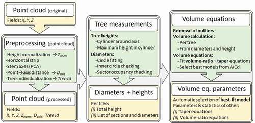
Figure 1 shows a workflow of the methodology detailing the steps involved the automatic parametrization of volume equations, including the input/output data needed and the procedures to be followed. In Section 2.1, the procedure for obtaining h and d_i in a fully automatic way from the TLS point cloud is explained in detail, including the identification and individualization of the stems, and the subsequent estimation of their geolocation. Section 2.2 details the procedure followed for the parametrization of the volume equations.

Figure 1. Workflow of the methodology proposed for the volume equations parametrization from TLS point clouds (Input/output data are shown in yellow and procedures in green)

2.1 Automatic estimation of dendrometric variables

2.1.1 Preprocessing of point cloud data

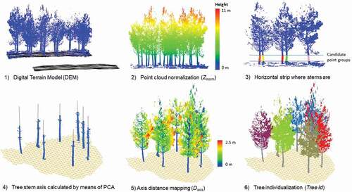
This part of the methodology encompasses all the steps that need to be followed to process the 3D point cloud prior to the automatic estimation of d_i and h: the aim is to automatically detect individual trees in the plot, then isolate and identify all points belonging to each tree and extract those points, which are along the stem. The workflow can be itemized as follows (see Figure 2).

1. Construction of a digital elevation model (DEM) to define the ground.

2. Height normalization of the point cloud to obtain Z coordinate, which refers to the ground (Z_norm).

3. Selection of candidate point groups along a horizontal strip (equal height from the horizontal ground), and where no scrub or branches are expected, on the basis of clustering of points using the DBSCAN algorithm (Birant and Kut 2007). The consistency of the groups in the horizontal strip is checked according to the methods described in Cabo et al. (2018a; 2018b).

4. Location of stem axis through the determination of the centroid and PC1 of detected stems: The methodology assumes that candidate tree stems are essentially linear features. As such, in the principal component (PC) analysis of the XYZ coordinates of each stem-candidate point group, the first PC (PC1) aligns with the direction of the maximum variance from the XYZ coordinates of each group. Then, PC1 is used to define the direction of each stem axis. The other two principal components (PC2 and PC3) are, by definition, perpendicular to each other and to PC1 (Oviedo-de et al. 2021) and can therefore be used as local/tree coordinate axes to calculate the distance of any point from the PC1 axis.

5. Calculation and storage of distances from each point to the closest axis: D_axis This has various applications, but the most obvious is that it allows the points of each tree to be filtered by their distance from the axis, making the separation of the main parts of each individual tree into crown/branches and stem relatively straightforward.

6. Tree individualization. All the points are assigned and linked to their closest axis (Tree Id)

Figure 2. Workflow for the identification of tree stems prior to automatic estimation of d_i and h. 1) DEM generation 2) Point cloud normalization (Z_norm) 3) Strip on the height normalized point cloud where the groups of candidate points likely to be tree stems are identified 4) Tree stem axes resulting from PCA analysis, where the PC1 is represented by a red line 5) Axis distance mapping of each tree (D_axis) 6) Tree individualization procedure, where all the points are labeled with a tree identifier (Tree Id)

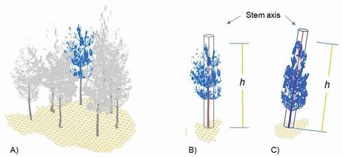
2.1.2 Tree height estimation

The estimation of tree height is based on the determination of the highest point in the crown in the proximity of each stem axis. For this, the points belonging to each tree (Figure 3A) are first clustered. From the resulting groups, those that are few in number and far from the stem, which may correspond to noise, artifacts, or canopy from higher neighbor trees, are automatically removed. The remaining points are filtered by distance from the tree axis in order to only consider those closest to the axis for the tree height estimation. This is done based on a threshold distance that delimits a cylinder around the top part of the tree, and can be varied for different species, conditions, or environments. h is finally estimated as the elevation above the ground of the highest point inside the cylinder (Figure 3B), which reduces the probability that h corresponds to the top of another higher tree, and allows appropriate estimations, even for tilted trees (Figure 3C). A default distance threshold value can be set as half of the average distance between neighbor trees in the plot. However, this value can be altered, generally reduced, if the stems are essentially straight and/or there is a high diversity in terms of tree height within the plot.

Figure 3. Tree height estimation procedure, where h is estimated for each individualized tree (A) as the highest point within the area of a delimited cylinder around the tree axis after noise filtering (B) and which is also valid for tilted trees (C)

2.1.3 Diameter estimation along the stem

The tree stem is initially segmented by extracting the points that are within a certain distance of each axis. This distance is set as the maximum stem radius expected in the plot. Then, diameters at different heights along each stem (d_i) are measured at a user defined interval starting from the ground (Figure 4A). To do so, each d_i is measured in a slice, which comprises all the points in a thin horizontal section of stem of uniform thickness. The maximum height with points in these sections strongly depends on the quality of the results obtained in the stem filtering step, which, in turn, is mainly dependent on occlusions, the point cloud density and the presence of artifacts around the stem, such as branches or understory. These three factors are interrelated and their influence on the resulting d_i is expected to be stronger in the upper sections of the stem. As well as the height interval for slice extraction, the thickness of the slices and the upper height limit can be specifically set for different species and/or conditions, environments or studies (Figure 4B).

Figure 4. A) Cross-sections along the stem B) Detail of stem slices showing height interval for their extraction, and their thickness C) Circle fitting to the points of a stem slice

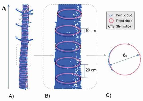
For the initial diameter estimation, the algorithm computes the diameters by fitting a circle to the points in each slice in each tree stem (Figure 4C). The circle fitting method is described in detail in Cabo et al. (2018a;b). The algorithm calculates the diameter and the X and Y coordinates of each section center, thus their position along the stem is defined and stored.

2.1.3.1 Automatic identification and labeling of anomalous sections

Frequently, the horizontal sections at different heights used to fit the circles contain points that do not belong to the stem but to other parts of the tree, such as branches, leaves or other artifacts. In those cases, the circle fitting may result in an erroneous estimation of the stem radius (r). The algorithm includes two complementary functions that allow, on the one hand, the identification and labeling of the anomalous sections, and, on the other, automatic correction in those cases where it is possible. Both functions are explained in detail below:

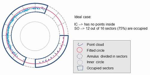
1. Inner circle (IC): this function was presented for the first time in Cabo et al. (2018a). Here, a concentric inner circle with radius r’ = r/2 is set up in the fitted section (Figure 5). If the position and size of the circle fitted is correct, no points are expected inside the inner circle.

2. Sector occupancy (SO): this function is based on the assumption that the points within a section follow a close-to-circular distribution and, except in cases of very severe occlusions, almost half of each tree section should be covered by points if it is measured from only one TLS setup, but more if it its measured from several setups. In order to verify that the circle fitting is compatible with this point coverage around the stem sections, an annulus divided into sectors is created around the position of each initially fitted circle (Figure 5). The width of the annulus can be varied if irregularities on the stem/bark are expected. If the position and size of the circle fit is correct, at least half minus one of the sectors should be occupied by points: this also allows circle fittings in stem sections that are only reached from one scan position, while the shape of the point group is continuously checked.

Figure 5. Checking functions of the circle fitting step in each section (IC +SO) showing an example of an ideal case, where the section would be labeled as correct

If in the first circle fitting of a section there are no points in the inner circle, and there are sufficient sectors occupied, the diameter estimation is considered correct. However, if there are points within the inner circle, or there are not sufficient sectors occupied in the annulus, it is highly probable that the diameter fitting is not correct. To resolve this, all the points within the section are clustered based on the distance between them. Then, the circle fitting is carried out again using only the cluster with the largest number of points, which is more likely to contain a higher percentage of points on the stem (Cabo et al. 2018a). This gives a new estimation for the diameter and position of the section of the stem. The new circle fitting is then checked again (i.e. IC and SO).

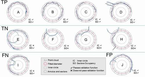
If a section passes the validation functions (either in the first or second round), it is labeled as “correct (C).” If both the first and second round of validation functions fail, the section is labeled as “flagged (F).” If in the first or the second round of validation functions there are not enough points to perform the circle fitting, the section is labeled as “not enough data (ND).”

Figure 6 shows 10 different hypothetical section scenarios and the behavior of the circle fitting and validation functions in each case. They are classified into four groups: True positives (TP), True negatives (TN), False positives (FP) and False negatives (FN). TP are correct estimations (from the first or second fitting round) and they are automatically stored as correct diameters (Figure 6. (A, B, C, D)). TN (i.e. those sections correctly labeled as F or ND) can be either left to be inspected visually by an operator or eliminated straightaway (Figure 6. (E, F, G, H)). FP and FN correspond to rare situations in which the algorithm would wrongly classify the results. For example, Figure 6I corresponds to an irregular stem section, while Figure 6J represents a branch with a quasi-circular section. However, these specific misassignments could be avoided by changing the parameters of the checking functions/tests (diameter of the inner circle, annulus width, and/or minimum number of occupied sectors).

Figure 6. Algorithm for diameter estimation performance when labeling sections. Sections can be classified into 4 categories, TP) True positives: labeled as C when they indeed are; TN) True negatives: labeled as F when they indeed are; FP) False positives: labeled as C when they should be F; and FN) False Negative: labeled as F when they should be C

2.2 Parametrization of volume equations

The merchantable volume can be calculated using different types of volume equations: mainly stem taper and volume-ratio equations, which are similar in terms of accuracy with respect to merchantable volume. In order to parametrize either of them, it is necessary to have a longitudinal data structure, that is, multiple diameter measurements for each individual at different heights along the stem (d_i, h_i) as well as the total height (h). The estimated dbh, d_i and h obtained from TLS data following the methodology described are used as input values to estimate merchantable volume using volume equations. For each type of volume equation, a large number of models (i.e. different specific expressions of the general volume equation) and parameter estimation approaches have been proposed in recent decades (Westfall and Scott 2010).

The first type of equation, a system of taper and volume equations, describe stem taper by providing (i) a taper equation with the diameter at any point along the stem or the height of the stem for a fixed diameter (eq.1), (ii) merchantable volume to any top diameter and from any height or individual volume for logs of any length at any height above the ground (eq.2) and (iii) total volume by integration of taper equation (eq.3). Taper equations can be classified into: simple taper equations, segmented taper equations and variable exponent taper equations. Of these, segmented taper equations have the greatest flexibility, as well as the capacity to describe the total volume efficiently (Pang et al. 2016). Ideally, a taper equation should be compatible, meaning that the volume computed by integration of the taper equation should be equal to that calculated by a total volume equation (Clutter 1980; Demaerschalk 1972). The specific model included in this work, that proposed by Fang, Borders, and Bailey (2000), meets this requirement as it includes a segmented taper equation (specific to f_1, eq.1), and complementary formulations to directly calculate total and merchantable volumes (specific to f_2, eq.2; specific to f_3, eq.3).

(eq. 1) $d_i=f_1\left(dbh,h,h_i\right)$(eq. 1)

(eq. 2) $v_i=f_2\left(dbh,h,d_i\right)$(eq. 2)

(eq. 3) $v=f_3\left(dbh,h\right)$(eq. 3)

It is important to consider that, in spite of the versatility and accuracy of stem taper equations, their practical use is limited unless they are embedded within a computer program (Larsen 2017). Moreover, when the data source is TLS, it is highly probable that the convergence in the iterations needed to calibrate the taper equation could be compromised due to the difficulty of d_i extraction in the upper stem because of branch occlusions in the crown, which leads to poor delimitation of the stem profile.

The second type of equations, volume ratio equations are, in contrast to taper equations, directly targeted at estimating wood volume up to a predefined diameter depending on its merchantable volume. They are very easy to both develop and use (Crecente-Campo, Alboreca, and Ulises 2009), and a hypothetical lack of upper stem data would not have a strong influence on their parametrization. Volume estimations from volume ratio equations, whose general expression is shown in eqs. 4–6, are based on the combined use of two equations – a total volume equation ($v$) (eq. 4) and a ratio equation, R_i (eq. 5) – to estimate the portion of volume up to a certain point (limit diameter d_i or height h_i) with values from 0 to 1, and, as such, the merchantable volume ($v_i$) is their product (eq. 6):

(eq. 4) $v=g_1\left(dbh,h\right)$(eq. 4)

(eq. 5) $R_i=g_2\left(dbh,d_i\right)$(eq. 5)

(eq. 6) $v_i=v.R_i$(eq. 6)

The algorithm developed in the current work, includes five total volume models (v; specific to g_1, eq.4) and four ratio models (R_i; specific to g_2, eq.5). The five specific total volume models (v, g1) are the linearized allometric model and four other models proposed by Spurr (1952): combined variable, generalized combined variable, quadratic, and cubic polynomial. The four ratio models (R_i; g_2, eq.5) included are the ones described in Burkhart (1977); Clark and Thomas (1984); Reed and Green (1984); Van Deusen, Sullivan, and Matvey (1981). Finally, the algorithm processes all the models and selects and integrates one of the total volume models (eq.4) and one of the ratio models (eq.5) into a volume ratio equation (eq.6), based on statistical criteria.

Considering all the above, the steps implemented in the algorithm are synthesized as follows:

1. In the first step, outliers in the stem analysis data (d_i, h_i) are detected following the systematic procedure proposed by Bi and Long (2001). A nonparametric taper curve is fitted using local regression with a typical smoothing factor value (0.25). Then, those values, which fall below a point equivalent to the lower quartile minus twice the interquartile range, or above a point corresponding to the upper quartile plus twice the interquartile range were removed owing to the fact that most of these data points correspond to stem deformations, and volume equations are not intended for deformed trees (Rodríguez, Torre, and Oviedo 2015).

2. The models implemented in the methodology (stem taper equation and the volume ratio models) are fitted and the algorithm calculates the values and significance of parameters (fitting by generalized least squares for non-linear models), the goodness-of-fit statistics of every model (coefficient of determination R², root mean square error RMSE, Akaike´s information criterion, AIC) are used to select the best model and measure the quality of the fittings, which can also be checked by graphical analysis (residual versus predicted values and predicted versus observed values and a scatterplot of relative diameter (d_i/dbh) vs relative height (h_i/h)).

3. After the debugging of the data set, total volume is calculated using a cone equation for the top section and, for each log, the Smalian equation (a formula that calculates the volume for each log by multiplying the average of the areas of the two end cross-sections by the section’s length). This total volume then becomes the dependent variable in the parametrization of the different equations.

4. The algorithm automatically selects the model with the lowest AICd (that is, the smallest AIC value in the set of models) where all parameters are significant as its candidate for the final merchantable volume equation. The user can either accept the algorithm choice or reject it and select any of the other proposed models according to their own preferences or specific requirements on the basis of all the goodness-of-fit statistics and graphical behavior of each model.

3. Case study

3.1 Study area and data

The methodology explained above was tested in a coniferous stand (Pinus pinaster) located in the autonomous region of Asturias (Figure 7A), where Pinus pinaster is the third species in terms of wood volume logging, representing 21% of total coniferous wood felled in Asturias (SADEI 2018).

Figure 7. A) Location of the study area B) Schema of the real distribution of the scans and the spheres in the test case plot C) Pinus pinaster stand and understory within the test case plot D) 3D representation of size and slope of the test case plot

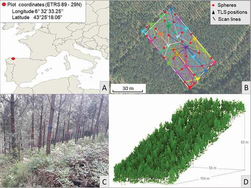
The study plot, which has an approximate area of 5700 m² (Figure 7B), is part of a breeding program where the growth of different families and provenances of Pinus pinaster is being evaluated (RTA2017-00063-C04-02, 2017). Initially, in 2005, 900 trees were planted following a gridded distribution. A thinning treatment was made in 2018, reducing the number of trees to 428. Regarding the stand characteristics, density is 806 trees/ha with an average dbh and h of 18 cm and 10.5 m, respectively, while the average canopy cover fraction is 44%. The terrain is irregular with a slope of 60% and dense cover of different species of scrub such as Ulex, Ericas, Pteridium among others (average height is 50 cm, canopy cover is 80%) (Figure 7C).

Data acquisition was carried out in November 2018 with a TLS model FAROFocus3D (Faro 2018). In total, 24 scans were necessary to ensure the full coverage of the study area and minimize the effect of occlusions. With the aim of merging the point clouds of individual scans into a unified coordinate system, polystyrene spheres of 25 cm diameter fixed to surveying rods were used. Also, the position of the spheres was measured in the field using GNSS (Global Navigation Satellite System), which has an accuracy of 1 cm, thereby ensuring that the unified point cloud had absolute coordinates. The RMSE of the registration was 4 mm, and the final matched point cloud obtained for all scans was approximately 150 million points, after removing duplicates within 6 mm. The scanning distribution is shown in Figure 7B. Finally, for all trees within the plot, dbh was measured in the field with a caliper (dbh_f) to the nearest 1 mm and total height (h_f) to the nearest 10 cm, using a digital hypsometer (Vertex IV 360º).

3.2 Assessing algorithm performance

The performance of the algorithm was assessed from two perspectives: tree detection rates and deviation in the estimation of diameters and tree heights. Tree detection rates were evaluated in terms of completeness and correctness with respect to the tree locations measured with the GNSS+Total station. Completeness was computed as the proportion of the trees within the plot that were detected by the algorithm (number of correctly detected trees divided by the total number of trees in the dataset) and Correctness was calculated as the proportion of elements identified as trees by the algorithm that were actual trees (number of correctly detected trees divided by the total number of elements detected as trees in the dataset). The deviation in the estimation of both diameter measurements, dbh and d_i, and height, h, was evaluated by comparing the results obtained from the algorithm and the values obtained using (i) traditional inventory methods and (ii) manual/visual measurements of the point cloud data.

In order to obtain the manual/visual measurements, a graphic interface was designed and implemented.

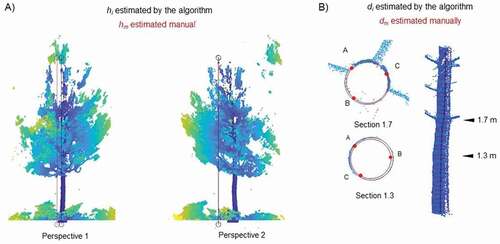
1. For manual tree height estimations (h_m) each tree is always shown from two different perspectives and the user can identify the highest point from both perspectives before selecting which to use, ensuring misassignments are avoided (e.g. if ‘Perspective 1ʹ in Figure 8A was the only available perspective of that specific tree, the h_m estimation would be wrong). The elevation of the selected point above the ground is stored as the total height of each individual.

2. For manual diameter (d_m) estimations, the horizontal distribution of the points included in each section is graphically displayed on the screen. Over each section, the user can draw 3 points (A, B, C) along the section contour, so that a circumference is automatically fitted to them (Figure 8B), after which the diameter and the coordinates of the fitted circle are stored. In the case of dbh, the deviation in the diameter estimated by the algorithm is also calculated by comparing it with the direct measurements in the field made with a caliper (428 sections: one per tree). In the case of the diameters along the stem, the algorithm estimations are compared with the manual measurements from the point cloud (9844 sections: 428 trees X 23 sections).

Figure 8. A) Manual total height estimation in the point cloud by marking the highest point in the cloud from two different perspectives B) Manual estimation diameter at different heights in the point cloud, by drawing 3 points (A, B, C) around the section contour

With the aim of minimizing the influence of the operator on the estimations, all height measurement and diameter fitting processes were conducted twice, each time by a different operator (Op 1 and Op 2).

3.3 Experimental results for automatic estimation of dendrometric variables

3.3.1 Stem detection rate

All the features detected as trees were actual trees with no false positives present, therefore, the correctness of the algorithm is 100% for the dataset. In regards to completeness, only 14 trees of the total 428 remained undetected, giving a value of 97%.

3.3.2 Total height

The algorithm automatically measured the total height of 98% of the trees. The average values obtained by the algorithm (h), by traditional inventory methods (h_f) and by manual measurement in the point cloud (h_m) as well as their standard deviation, are shown in Table 1. RMSE obtained when comparing h with h_f was 1.52 m.

Table 1. Mean and standard deviation (in meters) of the total height obtained from: algorithm (h), traditional inventory methods (h_f) and manual measurements of the point cloud data (h_m)

	h	hf	hm
Mean	8.78	10.29	8.72
Standard deviation	1.44	1.48	1.43

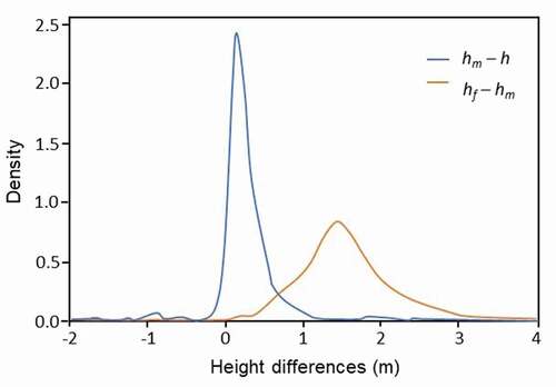
Figure 9A shows the differences analyzed tree by tree. More precisely, it shows probability density functions for the differences between h, h_f, and h_m. The differences between h and the h_m are less than 0.5 m for 83% of the trees, and less than 1 m for 94%, meaning that the operator and the algorithm each estimate a very similar height in the vast majority of cases. Although differences between h_f and h_m are higher, they are less than 2 m in 80% of cases.

Figure 9. A) Probability density functions for height differences comparing h_m versus h (blue line) and h_f versus h_m (orange line)

3.3.3 Diameters along the stem

In this dataset, due to the complexity of the forest stand structure (young trees with a great number of branches, along with high stand density and steep terrain; Figure 10A), the automatic estimation of diameters was carried out from 0.5 to 4.9 m in height (i.e. from the average height of the dense understory to approximately half the average height of the trees in the plot; Figure 10B). The circle fittings were computed for sections with a thickness of 5 cm and spaced 20 cm apart vertically (i.e. 23 sections per tree; Figure 10C)

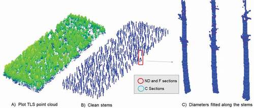
Figure 10. Visual results obtained by the algorithm for the diameter fitting in the study plot: (A) initial point cloud (B) clean stems (C) detail of circle fitting along the stem

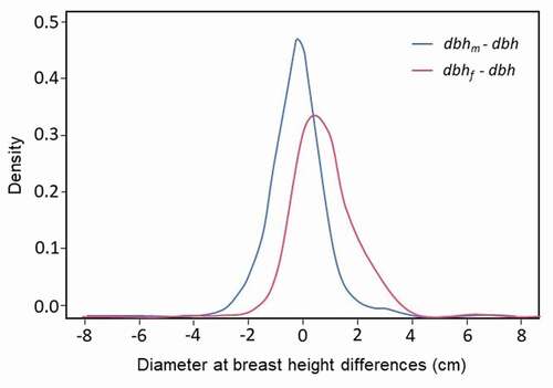
Regarding dbh, the algorithm measured it fully automatically in 93% of the trees within the plot, while in the remaining 7%, diameter fitting was not possible or was labeled as F or ND by the validation functions. The dbh average value was 17.27 (±3.2 cm) and the RMSE was 1.14 cm when compared with dbh_f. In absolute terms, 56% of the trees have an error value lower than 1 cm, and this increases to 82% for an error value of less than 2 cm. The distribution of the size of the differences in diameter estimation is shown in Figure 11 (pink line).

Figure 11. Probability density functions for diameter at breast height differences comparing dbh_m versus dbh (blue line) and dbh_f versus dbh (pink line)

Figure 12 shows the comparison of the diameters along the stem estimations obtained by the algorithm and the manual measurements carried out by the two operators. This comparison has a double aim: (i) comparing operator 1 and operator 2 provides information about the disparity of the different reference measurements and allows the identification and elimination of outliers (in cases where the differences between operators are high) and (ii) the comparison between the algorithm and the operators provides an estimation of the accuracy of the method while allowing the subjectivity associated with the operators’ measurements to be considered.

Figure 12. Boxplots of the differences between A) manual estimation of operator 1 (Op 1) and operator 2 (Op 2); B) and C) comparison of the manual estimation of Op1 and Op2, respectively, with algorithm estimation excluding sections flagged as candidates for review. Q1 and Q2 represent the percentiles, and min and max refer to 1.5 times the interquartile range in mm from the upper and lower quartiles respectively. On the right of each boxplot the blue line represents the number of sections (as a percentage) that were used to build the boxes for each section

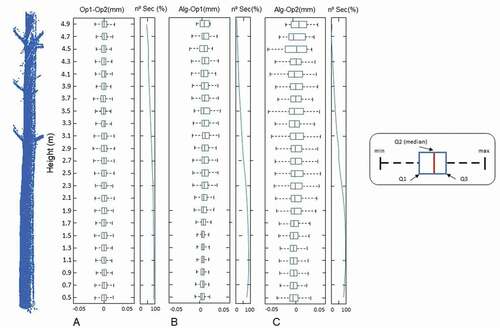
Specifically, Figure 12A shows the differences between the estimations of the two operators in those sections where both could see and draw a circle. These differences are approximately of the same order and remain constant along the whole stem: they show apparent symmetric distributions and no bias at any specific height.

Figure 12B and 12C show the differences between the diameter estimations along the stems as calculated by the operators and by the algorithm in the sections that were not flagged for review or elimination by the algorithm. The differences between the two operators are very small according to the average interquartile range (8.2 mm) and remain constant along the stem. However, when the estimations of each operator are compared to those from the algorithm, the interquartile range is slightly higher (Op1-alg: 11.2 mm and Op2-alg: 24.0 mm) and the difference increases with the height of the section. Specifically in the case of dbh, RMSE was 1.02 cm when compared with dbh_m and the distribution of the size of the differences in diameter estimation is shown in Figure 11 (blue line). On the right of each boxplot the blue line represents the proportion of sections that were used to build the boxplots for each section. The general tendency in each of the 4 boxplots is for the number of sections to decrease with height. This is to be expected because of the presence of low branches and the high density of trees, a combination, which makes diameter fittings more difficult higher up the stem, particularly when the branches of the crown begin to appear (at around 2.5 m in this test case).

3.3.3.1 Anomaly detection in stem sections

Figure 13 shows the distribution of the sections along the stem in terms of how the algorithm classifies them: correct sections (C: gray), flagged (F: magenta), and those where there was not enough data to compute the circle fitting (ND: blue). Also, to assess the performance of the algorithm when identifying ND, and to compare the results with the manual estimations, ND sections have been subdivided into NDa (not enough points for either circle fitting or visual/manual estimation: dark blue) and NDb (not enough points for circle fitting, but sufficient for visual/manual estimation by the operators: pale blue).

Figure 13. Labeling results obtained by the algorithm expressed in terms of percentage of sections classified into each category

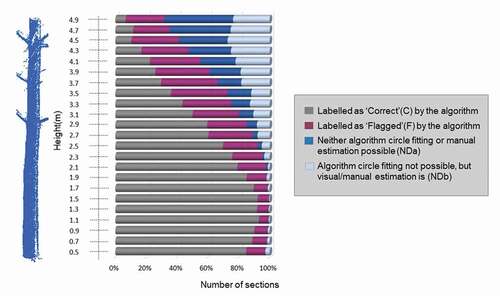
As demonstrated in Figure 13, in general terms, the proportion of both F and ND sections is lowest around breast height (1.2–1.6 m) where stems are less affected by occlusions from understory or tree branches, and, in addition, the incidence angle of the laser beams is in general more favorable. In these sections, more than 90% of the diameter estimations are labeled as C, and less than 2% as ND.

The proportion of F sections increases steadily on either side of breast height (i.e. below 1.1. and above 1.5 m), and remains stable above approximately 2.5 m, the average height of the first branches. Conversely, the proportion of ND increases consistently with height from breast height (same increase rate for NDa and NDb up to the last two sections, where NDa becomes much larger than NDb)

3.4 Experimental results for parametrization of volume equations

Selected taper and volume ratio equations were fitted using two datasets that include the following variables for each tree: d_i, h_i and h. The data sets differ in the way in which these three variables have been calculated. In the first (hereafter, “Automatic”), all the variables were estimated automatically by the algorithm. The second (hereafter, “Supervised”), contains the same data as the Automatic, but those sections it labeled as F or ND were substituted by the diameter manually estimated by an operator, i.e. the data from Op1 and Op2 that was also used to evaluate the automatic diameter estimations. There were a small number of measurements, which were very different between the operators, and these were considered outliers, and removed from the dataset. However, in general, measurements from the two operators were very close (<5 mm) so the use of data from either of them would provide virtually the same result. On this basis, the diameter from either Op1 or Op2 was selected randomly for each section.

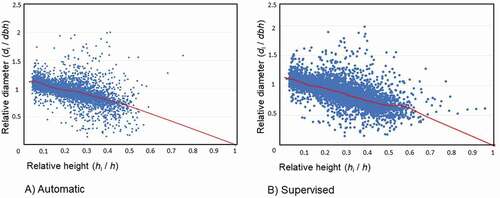
Figure 14 shows the scatter plot of the relative diameters (d_i /dbh) vs relative heights (h_i/h) that were used for the parameterization of the merchantable volume equations. In both cases there is a reduction in the number of sections that were available for the model parametrization in the upper part of the stems, especially in the top third of the stem. For the supervised data the situation is slightly better than in the Automatic, because there are more sections in the band of relative height (h_i/h), corresponding to 0.60 to 0.80 whereas in the Automatic data there are virtually no sections in that interval. Moreover, there are more sections providing results in the Supervised data and a smaller proportion of outliers than in the Automatic data (7384 vs 5362 sections and a proportion of outliers of 9.7% vs 11.6.%, respectively).

Figure 14. Scatterplots of relative diameter (d_i/dbh) vs relative height (h_i/h), with a local regression smoothing curve (red line) for the two datasets used in fitting merchantable volume equations Note: point (1,0) represents the final section of the stem, where d_i = 0 (d_i/d = 0) and h_i = h (h_i/h = 1)

For both datasets, the algorithm offered the following outputs: parameter estimation, goodness-of-fit statistics and graphical analysis (residual and predicted vs. observed data) of the merchantable volume equations. Looking first at the taper equation system, it did not converge in either of the two data sets due to the lack of sections in the upper third of the stem. From among the volume ratio equations, the algorithm selected for each data set was that with the lowest AICd and where all parameters were significant, which in this particular case was the allometric volume equation (eq. 7) and the ratio equation proposed by Clark and Thomas (1984) (eq. 8).

(eq. 7) $v=b_{0}db{h}^{b1}{h}^{b2}$(eq. 7)

(eq. 8) $R_i=exp(b_3{d}_i^{b4}db{h}^{b5})$(eq. 8)

where v is total over bark stem volume (m³), calculated as the sum of the volume of all the logs within the stem, and the top of the tree; R_i is the proportion of total volume accounted for at diameter (d_i); dbh is diameter at breast height (cm); d_i over bark diameter at height h_i (cm); h is total tree height in m, and b₀, b₁, b₂, b₃, b₄ and b₅ are the parameters to be estimated.

Table 2 shows the number of sections used and the comparison of the goodness-of-fit statistics for the volume ratio equation selected by the algorithm, for each of the datasets.

Table 2. Goodness-of-fit statistics of the model fitted in the different data sets

	Data set	n	P	RMSE	R^2
Total volume equation	Supervised	7382	3	0.0149	0.8480
	Automatic	5362	3	0.0233	0.6714
Ratio equation	Supervised	7384	3	0.1630	0.6759
	Automatic	5362	3	0.1747	0.6382

Note: n is the number of sections used for the equation fitting, P is the number of parameters in the model, RMSE root mean square error, and R² is the coefficient of determination.

The Supervised dataset gives better results than the Automatic, especially in the case of the total volume equation. The results demonstrate that a low number of sections, and more specifically their absence in the upper third of the tree, is what is responsible for the drop in the values of the model statistics. Finally, Table 3 shows the estimation of the model parameters, which were significant at the 5% level in the two datasets.

Table 3. Parameter estimated for the models fitted in the different data sets

Data set	Total volume equation			Ratio equation
	b0	b1	b2	b3	b4	b5
Supervised	0.00008	1.833	0.7875	−0.5664	4.044	−3.797
Automatic	0.000091	1.659	0.9396	−0.7997	3.946	−3.814

Note: b₀, b₁, b₂, b₃, b₄ and b₅ are the estimated parameters in the volume ratio equations.

4. Discussion

4.1 Comparison with previous work

Comparing the performance of the methodology employed in this work with previous studies is not straightforward as plot size, tree density, forest structure, etc. vary between trials (Cabo et al. 2018a) and all have a strong influence on the results. Moreover, the test case plot has the additional difficulties of high slope, young, and therefore small trees, a tendency of the trees to tortuosity and, particularly, the high density of branches and understory. Despite this, it is possible to establish a range of values obtained by other authors for each dendrometric variable and for volume equations that can serve as a reference for discussion. Regarding tree detection, it is strongly influenced by stem density (Liang and Hyyppä 2013; Thies et al. 2004): the lower the tree density in the sample plot, the higher the detection rate of the stems (Chen et al. 2009). According to Liang et al. (2016), in sparse forests (100–200 stems/ha), the detection rate may reach 100%, while in a forest with a stem density of over 1000 stems/ha, the stem detection rate is generally around 70%. The results obtained in this study for stem individualization are extremely good, with 97% success in a plot with 806 stems/ha. The approach of selecting only the points close to the projection of the stem, based on the estimation of a linear axis for each tree, indeed outperforms previous works by some of the authors (Cabo et al. 2018a; 2018b) as it reduces the probability of assigning a tree the height of a higher neighbor tree and eliminates points from branches, leaves, or other features around the stem for a more effective diameter estimation.

4.2 Tree height estimation

Regarding the results obtained for the calculation of h, most of the differences between the algorithm estimations and the field measurements are between 1 and 2 m. Tree height underestimation using TLS datasets is a common issue (Olofsson and Holmgren 2016), explained by the fact that the light beam of the sensor is not capable of reaching the top of the crowns, due to foliage obstruction, so the treetops are very often not well defined in the resulting point cloud. Nevertheless, when comparing h with h_m, the differences are barely noticeable (6 cm of difference between average values), which indicates that the limitation does not lie with the algorithm, but rather in the nature and quality of the data itself. In cases where h needs to be estimated with high accuracy TLS data could be complemented with aerial data, such as LiDAR (Hadas et al. 2017; LaRue et al. 2020; Puletti et al. 2020) or photogrammetric data (Aicardi et al. 2016; Tian et al. 2019) or with a subsample of field measurements in those cases where no remote sensing data is available.

4.3 Diameter estimation

Concerning the dbh versus dbh_f comparison, RMSE was 1.14 cm, which is compatible with the values of between 0.71 and 2.64 cm reported in previous studies (Hollaus, Mokroš, and Wang 2019). The difference between Automatic and manual procedures as diameters along the stem increases is also consistent with previous research (Henning and Radtke 2006; Maas et al. 2008) and can be attributed to low point density in higher parts of the stem, the smaller object surface area and obstructions caused by branches and foliage (Liang and Hyyppä 2013). This fact also explains why the most accurate estimations occur in the intermediate part of the tree (between 0.7 and 2.9 m, approximately), which is the interval considered to be “occlusion free.” The distribution of anomalous sections (F and ND) follows the same pattern, that is, they are more frequent in the lowest and highest parts of the stem. This problem with diameter estimation in the upper and lower sections could possibly be improved by scanning at higher resolutions, which could lead to better penetration of the foliage, and more laser points. However, any improvement would probably be limited because higher resolutions would still not reduce the occlusion effect (Liang et al. 2016). Stem profile measurement could also be improved by combining diameter measurements retrieved from different sources, or, as shown in the supervised method used in the test case, by incorporating visual checking or manual fitting in challenging sections if very high accuracy is needed. This might include the possibility of selecting the trees to be used in the parametrization of the equations.

4.4 Parametrization of volume equations

For the parametrization of the merchantable volume equations, the number of sections available, especially in the upper third of the stem, clearly influences the convergence of the stem taper equation and the accuracy of volume estimations. In this particular test case, the use of supervised data improves on the results obtained with the Automatic data, resulting in an increase of R² both in the stem volume equations (from 0.67 to 0.85) and in the ratio equations (from 0.64 to 0.68), as well as the reduction of RMSE (from 0.0233 to 0.0149 m³). When these results are compared with those obtained by destructive techniques in Pinus pinaster, where R² for stem volume equations ranges between 0.91 and 0.98 (Alegria and Margarida 2011; Yousefpour et al. 2012) and for volume-ratio equations is between 0.80 and 0.89 (Teshome 2005), the values for the same parameter obtained in this study might seem to be low. However, a comparison in absolute terms is not realistic because: (i) in destructive techniques only healthy and standard-shaped trees for which there is a full range of measurements along the stem are considered and (ii) in contrast to this study, where all the trees in the plot were considered, in destructive sampling, young trees with erratic growth are generally excluded. Consequently, it is only to be expected that results would be better in study plots with adult trees, low-density understory, and the reduced presence of branches.

4.5 Algorithm implementation performance

In terms of time, destructive sampling is by far the most time-consuming step involved in the parametrization of volume equations by means of traditional techniques (Yu et al. 2013). In the case of TLS sampling, only one day would be necessary for a sample of 100–150 trees, which is the number of trees commonly used to adjust merchantable volume equations (Crecente-Campo, Alboreca, and Ulises 2009). The authors have estimated that only 3 minutes per tree (16GB RAM, i7 4-core 8 G processor) is needed to obtain the parametrized volume-ratio equation (including scanning field work), which is a substantial improvement in time compared to destructive methods. Furthermore, in the case of the supervised dataset, only 20 seconds was necessary to review a complete tree (i.e. 2.5 hours of intense work for all the trees in the test plot). Consequently, the supervised option is cost-effective in terms of time invested vs improvement in the merchantable volume equations.

4.6 Transferability of the method

This study is eminently methodological, and it has been applied and evaluated in a specific plot of Pinus pinaster to assess the performance of the method. The results from a single study plot can be transferred to others as long as they have similar characteristics to the test case plot. However, the strong point of the methodology presented here is that it provides the possibility of parametrizing the volume equations of any tree species or stand typology. The only requirement, is to scan an adequate number of trees (in one or several plots, depending on the scope of the application of the volume equations) so that the algorithm has the necessary input diameters and tree heights (from TLS point clouds) to parametrize the volume equations, after which the algorithm selects the most suitable equation for each case.

From the point cloud processing perspective, the basic principles of tree detection and diameter estimation have already been tested in plots with different characteristics in benchmark studies (Liang et al. 2018; Hollaus, Mokroš, and Wang 2019). These studies describe how more than 20 different algorithms work in a wide variety of scenarios (i.e. different point cloud and vegetation densities, plot configurations, and point cloud technologies) and provide very good results when compared with traditional field measurements. However, it is possible that fully automatic approaches for diameter estimations give poorer results in stands with very complex structural or orographic conditions (Liang et al. 2018; Cabo et al. 2018a, 2018b; Hollaus, Mokroš, and Wang 2019). In this sense, the methodology here offers contingency alternatives for such complex scenarios: it automatically analyses the coherence of the tree measurements (diameters along the stem), flags anomalous estimations and includes the possibility of the visual checking and correction of flagged measurements. Furthermore, this can be also applied in not-so-complex scenarios, when, for instance, there are few trees available in the TLS datasets and thus problematic or anomalous sections cannot be discarded. What is more, while the methodology selects the most appropriate option (based on statistical indicators: AICd), it also offers the possibility of selecting a different model, when, for instance, the reliability of a specific model has been demonstrated to be better for a particular species and/or plot configurations (Westfall and Scott 2010; Menéndez-Miguélez et al. 2014; Saarinen et al. 2019).

4.7 Influence of measurement errors

Regarding the management of possible measurement errors, in forest inventory modeling it is common to assume that the independent variables are free of measurement error (Morales-Hidalgo, Kleinn, and Scott 2017). Also, some studies have compared the impact of measurement errors on the parametrization of taper functions when using direct traditional methods and indirect nondestructive methods like TLS (Rodríguez, Torre, and Oviedo 2015; Marchi et al. 2020; Torresan et al. 2021). Most of these studies concluded that the errors are similar or that they are smaller when using indirect (i.e. remote and nondestructive) measurements. Nevertheless, considering an error model for the independent variables could reinforce the analysis, so this may be something worth exploring in future studies. In the specific case of this study, using error models for the independent variables would, however, affect the automation of the method, as it would involve the need for a specific error model for each scanner and/or stand characteristic, which would potentially impact the simplicity and usability of the method.

5. Conclusions

In this study, a fully automatic methodology for the parametrization of stem merchantable volume equations from TLS data was developed and tested. The methodology, applicable to any species or stand typology, automatically detects the trees within a plot, and measures diameters along the stem (d_i, including dbh) as well as total height (h) at the individual tree level. These variables are then used by the algorithm as direct inputs for the parametrization of a set of merchantable volume equations (one stem taper equation and several volume-ratio equations) from which the one with the lowest AICd is automatically selected. The methodology incorporates an automatic system for identifying and labeling stem sections, which present anomalous diameter estimations so that they can either be discarded or manually reviewed.

The methodology was tested in a dense Pinus pinaster plot with 428 trees, steep slopes, low branches and dense understory. The automatic estimations of tree height and diameter were compared with field data and manual measurements made on the point cloud data. The results show good tree height estimation, but a clear misrepresentation of treetops. As for diameters along the stem, the best estimations are in the intermediate part of the stem and have no apparent bias. Discrepancies with reference data, however, increase with height, as does the number of sections that are flagged for review or elimination. Consequently, the number of sections available for the merchantable volume equation fitting is reduced, especially in the upper third of the stem. This fact has a strong influence on both the type of merchantable volume equation that can be fitted, and the degree of uncertainty in the merchantable volume estimation.

In the test case, the manual review of sections flagged for review or elimination improved the volume estimation. Nevertheless, the results obtained using the fully automatic approach are still suitable for the parametrization of the equations when there is no need for a high degree of accuracy in the merchantable volume estimation Also, the nature of the methodology suggests that better results could be obtained with less challenging plots, but in order to achieve a well-founded analysis of the performance of the methodology, further analysis covering a wider range of test cases is needed.

Finally, it is important to note that TLS sampling overcomes the traditional drawbacks of destructive methods, providing a 3D reconstruction of the forest at the moment of the scan. This has many advantages such as multitemporal studies with various objectives, enabling new variables of interest to be studied retrospectively, and the possible estimation of other stem shape variables (closely related to wood quality).

Data and Codes Availability Statement

The data that support the findings of this study are available with the identifier 10.6084/m9.figshare.14046578 at the private link: https://figshare.com/s/50286f1ab59f5da937bd.

Acknowledgments

The authors wish to thank CETEMAS field workers (Manuel Alonso-Graña López and Ernesto Menéndez Álvarez) for carrying out the scanning of the whole plot. Thanks also to Ronnie Lendrum, scientific editor and proof-reader, for correcting the English of the manuscript.

Disclosure statement

No potential conflict of interest was reported by the author(s).

Additional information

Funding

This work was supported by the Instituto Nacional de Investigación y Tecnología Agraria y Alimentaria (INIA) in the framework of the RTA2017-00063-C04-02 (2017) project entitled : “Evaluation of relevant characters for the sustainable management ofPinus pinaster Ait. and their interaction under new climatic scenarios„ and by the UK Environment Research Council (NE/T001194/1).

References

- Aicardi, I., P. Dabove, A. M. Lingua, and M. Piras. 2016. “Integration between TLS and UAV Photogrammetry Techniques for Forestry Applications.” IForest-Biogeosciences and Forestry 10 (1): 41. SISEF-Italian Society of Silviculture and Forest Ecology. doihttps://doi.org/10.3832/ifor1780-009.
- Alegria, C., and T. Margarida. 2011. “A Set of Models for Individual Tree Merchantable Volume Prediction for Pinus Pinaster Aiton in Central Inland of Portugal.” European Journal of Forest Research 130 (5): 871–879. Springer. doihttps://doi.org/10.1007/s10342-011-0479-3.
- Bi, H., and Y. Long. 2001. “Flexible Taper Equation for Site-Specific Management of Pinus Radiata in New South Wales, Australia.” Forest Ecology and Management 148 (1–3): 79–91. Elsevier. doihttps://doi.org/10.1016/S0378-1127(00)00526-0.
- Birant, D., and A. Kut. 2007. “ST-DBSCAN: An Algorithm for Clustering Spatial–Temporal Data.” Data & Knowledge Engineering 60 (1): 208–221. doi:https://doi.org/10.1016/j.datak.2006.01.013.
- Burkhart, H. E. 1977. “Cubic-Foot Volume of Loblolly Pine to Any Merchantable Top Limit.” Southern Journal of Applied Forestry 1 (2): 7–9. Oxford University Press. doihttps://doi.org/10.1093/sjaf/1.2.7.
- Cabo, C., A. Kukko, S. García-Cortés, H. Kaartinen, J. Hyyppä, and O. Celestino. 2016. “An Algorithm for Automatic Road Asphalt Edge Delineation from Mobile Laser Scanner Data Using the Line Clouds Concept.” Remote Sensing 8 (9): 740. doi:https://doi.org/10.3390/rs8090740.
- Cabo, C., C. Ordóñez, C. A. López-Sánchez, and J. Armesto. 2018b. “Automatic Dendrometry: Tree Detection, Tree Height and Diameter Estimation Using Terrestrial Laser Scanning.” International Journal of Applied Earth Observation and Geoinformation 69: 164–174. doi:https://doi.org/10.1016/j.jag.2018.01.011.
- Cabo, C., D. P. Susana, P. Rodríguez-Gonzálvez, C. Ordóñez, and G.-A. Diego. 2018a. “Comparing Terrestrial Laser Scanning (TLS) and Wearable Laser Scanning (WLS) for Individual Tree Modeling at Plot Level.” Remote Sensing 10 (4): 540. doi:https://doi.org/10.3390/rs10040540.
- Calders, K., J. Adams, J. Armston, H. Bartholomeus, S. Bauwens, L. P. Bentley, J. Chave, F. M. Danson, M. Demol, and M. Disney. 2020. “Terrestrial Laser Scanning in Forest Ecology: Expanding the Horizon.” Remote Sensing of Environment 251: 112102. Elsevier. doi:https://doi.org/10.1016/j.rse.2020.112102.
- Cao, Q. V., H. E. Burkhart, and T. A. Max. 1980. “Evaluation of Two Methods for Cubic-Volume Prediction of Loblolly Pine to Any Merchantable Limit.” Forest Science 26 (1): 71–80. Oxford University Press. doihttps://doi.org/10.1093/forestscience/26.1.71.
- Chen, Y., S. Wei, L. Jing, and Z. Sun. 2009. “Hierarchical Object Oriented Classification Using Very High Resolution Imagery and LIDAR Data over Urban Areas.” Advances in Space Research 43 (7): 1101–1110. doi:https://doi.org/10.1016/j.asr.2008.11.008.
- Clark, A., and C. E. Thomas. 1984. “Weight Equations for Southern Tree Species: Where We are and What Is Needed.„ In: Daniels R. F., and P. H. Dunhan (Eds.), Proceedings of the 1983 southern forest biomass workshop, USDA Forest Service, Southern Forest Experimental Station, Ashevile, Northern Carolina, 100–106.
- Clutter, J. L. 1980. “Development of Taper Functions from Variable-Top Merchantable Volume Equations.” Forest Science 26 (1): 117–120. Oxford University Press.
- Corral-Rivas, J., U. Javier, S. Diéguez-Aranda, C. Rivas, and F. C. Dorado. 2007. “A Merchantable Volume System for Major Pine Species in El Salto, Durango (Mexico).” Forest Ecology and Management 238 (1–3): 118–129. doi:https://doi.org/10.1016/j.foreco.2006.09.074.
- Crecente-Campo, F., A. R. Alboreca, and D.-A. Ulises. 2009. “A Merchantable Volume System for Pinus Sylvestris L. In the Major Mountain Ranges of Spain.” Annals of Forest Science 66 (8): 808. doi:https://doi.org/10.1051/forest/2009078.
- Dassot, M., A. Colin, P. Santenoise, M. Fournier, and T. Constant. 2012. “Terrestrial Laser Scanning for Measuring the Solid Wood Volume, Including Branches, of Adult Standing Trees in the Forest Environment.” Computers and Electronics in Agriculture 89: 86–93. doi:https://doi.org/10.1016/j.compag.2012.08.005.
- Demaerschalk, J. P. 1972. “Converting Volume Equations to Compatible Taper Equations.” Forest Science 18 (3): 241–245. doi:https://doi.org/10.1093/forestscience/18.3.241.
- Fang, Z., B. E. Borders, and R. L. Bailey. 2000. “Compatible Volume-Taper Models for Loblolly and Slash Pine Based on a System with Segmented-Stem Form Factors.” Forest Science 46 (1): 1–12. doi:https://doi.org/10.1093/forestscience/46.1.1.
- Faro. 2018. http://www.faro.com (Accessed 31 April 2019).
- Fröhlich, C., and M. Mettenleiter. 2004. “Terrestrial Laser Scanning—New Perspectives in 3D Surveying.” International Archives of Photogrammetry, Remote Sensing and Spatial Information Sciences 36 (Part 8): W2.
- Gabriel, R. S. 2017. “The Use of Terrestrial Laser Scanning and Computer Vision in Tree Level Modelling.” Master Thesis. Oregon State University.
- González, Á., J. Gabriel, V. G. Klaus, and P. R. Hermosilla. 2001. “Modelización Del Crecimiento y La Evolución de Bosques.” IUFRO World Series 12: 242.
- Hackenberg, J., C. Morhart, J. Sheppard, H. Spiecker, and M. Disney. 2014. “Highly Accurate Tree Models Derived from Terrestrial Laser Scan Data: A Method Description.” Forests 5 (5): 1069–1105. doi:https://doi.org/10.3390/f5051069.
- Hadas, E., A. Borkowski, J. Estornell, and P. Tymkow. 2017. “Automatic Estimation of Olive Tree Dendrometric Parameters Based on Airborne Laser Scanning Data Using Alpha-Shape and Principal Component Analysis.” GIScience & Remote Sensing 54 (6): 898–917. Taylor & Francis. doihttps://doi.org/10.1080/15481603.2017.1351148.
- Hauglin, M., T. Gobakken, R. Astrup, L. Ene, and E. Na esset. 2014. “Estimating Single-Tree Crown Biomass of Norway Spruce by Airborne Laser Scanning: A Comparison of Methods with and without the Use of Terrestrial Laser Scanning to Obtain the Ground Reference Data.” Forests 5 (3): 384–403. doi:https://doi.org/10.3390/f5030384.
- Henning, J. G., and P. J. Radtke. 2006. “Detailed Stem Measu rements of Standing Trees from Ground-Based Scanning Lidar.” Forest Science 52 (1): 67–80. doi:https://doi.org/10.1093/forestscience/52.1.67.
- Hollaus, M., M. Mokroš, and Y. Wang. 2019. “International Benchmarking of Terrestrial Image-Based Point Clouds for Forestry.” In European Geosciences Union, General Assembly 2019, Vienna. Geophysical Research Abstracts, 21: 1–1.
- Holopainen, M., M. Vastaranta, V. Kankare, M. Räty, M. Vaaja, X. Liang, X. Yu, J. Hyyppä, H. Hyyppä, and R. Viitala. 2011. “Biomass Estimation of Individual Trees Using Stem and Crown Diameter TLS Measurements.” ISPRS-International Archives of the Photogrammetry, Remote Sensing and Spatial Information Sciences 3812: 91–95. doi:https://doi.org/10.5194/isprsarchives-XXXVIII-5-W12-91-2011.
- Jung, S.-E., D.-A. Kwak, T. Park, W.-K. Lee, and S. Yoo. 2011. “Estimating Crown Variables of Individual Trees Using Airborne and Terrestrial Laser Scanners.” Remote Sensing 3 (11): 2346–2363. doi:https://doi.org/10.3390/rs3112346.
- Kankare, V., J. Vauhkonen, T. Tanhuanpää, M. Holopainen, M. Vastaranta, M. Joensuu, A. Krooks, J. Hyyppä, H. Hyyppä, and P. Alho. 2014. “Accuracy in Estimation of Timber Assortments and Stem Distribution–A Comparison of Airborne and Terrestrial Laser Scanning Techniques.” ISPRS Journal of Photogrammetry and Remote Sensing 97: 89–97. doi:https://doi.org/10.1016/j.isprsjprs.2014.08.008.
- Larsen, D. R. 2017. “Simple Taper: Taper Equations for the Field Forester.” In: J. M. Kabrick, D. C. Dey, B. O. Knapp, D. R. Larsen, S. R. Shifley, and H. E. Stelzer, Eds. Proceedings of the 20th Central Hardwood Forest Conference; 2016 March 28-April 1; Columbia, MO. General Technical Report NRS-P-167. Newtown Square, PA: US Department of Agriculture, Forest Service, Northern Research Station, 265-278, 265–278.
- LaRue, E. A., F. W. Wagner, S. Fei, J. W. Atkins, R. T. Fahey, C. M. Gough, and B. S. Hardiman. 2020. “Compatibility of Aerial and Terrestrial LiDAR for Quantifying Forest Structural Diversity.” Remote Sensing 12 (9): 1407. Multidisciplinary Digital Publishing Institute. doihttps://doi.org/10.3390/rs12091407.
- Laurin, G. V., N. Puletti, W. Hawthorne, V. Liesenberg, P. Corona, D. Papale, Q. Chen, and R. Valentini. 2016. “Discrimination of Tropical Forest Types, Dominant Species, and Mapping of Functional Guilds by Hyperspectral and Simulated Multispectral Sentinel-2 Data.” Remote Sensing of Environment 176: 163–176. doi:https://doi.org/10.1016/j.rse.2016.01.017.
- Li, L., M. Xihan, M. Soma, P. Wan, Q. Jianbo, H. Ronghai, W. Zhang, Y. Tong, and G. Yan. 2020. “An Iterative-Mode Scan Design of Terrestrial Laser Scanning in Forests for Minimizing Occlusion Effects.” IEEE Transactions on Geoscience and Remote Sensing. IEEE. doi:https://doi.org/10.1109/TGRS.2020.3018643.
- Liang, X., and J. Hyyppä. 2013. “Automatic Stem Mapping by Merging Several Terrestrial Laser Scans at the Feature and Decision Levels.” Sensors 13 (2): 1614–1634. Multidisciplinary Digital Publishing Institute.
- Liang, X., J. Hyyppä, A. Kukko, H. Kaartinen, A. Jaakkola, and Y. Xiaowei. 2014. “The Use of a Mobile Laser Scanning System for Mapping Large Forest Plots.” IEEE Geoscience and Remote Sensing Letters 11 (9): 1504–1508. IEEE. doihttps://doi.org/10.1109/LGRS.2013.2297418.
- Liang, X., J. Hyyppä, H. Kaartinen, M. Holopainen, and T. Melkas. 2012. “Detecting Changes in Forest Structure over Time with Bi-Temporal Terrestrial Laser Scanning Data.” ISPRS International Journal of Geo-Information 1 (3): 242–255. Multidisciplinary Digital Publishing Institute. doihttps://doi.org/10.3390/ijgi1030242.
- Liang, X., J. Hyyppä, H. Kaartinen, M. Lehtomäki, J. Pyörälä, N. Pfeifer, M. Holopainen, G. Brolly, P. Francesco, and J. Hackenberg. 2018. “International Benchmarking of Terrestrial Laser Scanning Approaches for Forest Inventories.” ISPRS Journal of Photogrammetry and Remote Sensing 144: 137–179. doi:https://doi.org/10.1016/j.isprsjprs.2018.06.021.
- Liang, X., V. Kankare, J. Hyyppä, Y. Wang, A. Kukko, H. Haggrén, and Y. Xiaowei. 2016. “Terrestrial Laser Scanning in Forest Inventories.” ISPRS Journal of Photogrammetry and Remote Sensing 115 (May): 63–77. Theme issue “State-of-the-art in photogrammetry, remote sensing and spatial information science”. doihttps://doi.org/10.1016/j.isprsjprs.2016.01.006.
- Maas, H.-G., A. Bienert, S. Scheller, and E. Keane. 2008. “Automatic Forest Inventory Parameter Determination from Terrestrial Laser Scanner Data.” International Journal of Remote Sensing 29 (5): 1579–1593. doi:https://doi.org/10.1080/01431160701736406.
- Marchi, M., R. Scotti, G. Rinaldini, and P. Cantiani. 2020. “Taper Function for Pinus Nigra in Central Italy: Is a More Complex Computational System Required?.” Forests 11 (4): 405. doi:https://doi.org/10.3390/f11040405.
- Menéndez-Miguélez, M., E. Canga, P. Álvarez-Álvarez, and J. Majada. 2014. “Stem Taper Function for Sweet Chestnut (Castanea Sativa Mill.) Coppice Stands in Northwest Spain.” Annals of Forest Science 71 (7): 761–770. doi:https://doi.org/10.1007/s13595-014-0372-6.
- Mengesha, T., M. Hawkins, and M. Nieuwenhuis. 2015. “Validation of Terrestrial Laser Scanning Data Using Conventional Forest Inventory Methods.” European Journal of Forest Research 134 (2): 211–222. Springer. doihttps://doi.org/10.1007/s10342-014-0844-0.
- Mohammed, H. I., Z. Majid, and L. N. Izah. 2018. “Terrestrial Laser Scanning for Tree Parameters Inventory.” IOP Conference Series: Earth and Environmental Science, Kuala Lumpur, Malaysia; 169, (July), 012096. doi: https://doi.org/10.1088/1755-1315/169/1/012096.
- Morales-Hidalgo, D., C. Kleinn, and C. T. Scott. 2017. Voluntary Guidelines on National Forest Monitoring. FAO.
- Newnham, R. M. 1992. “Variable-Form Taper Functions for Four Alberta Tree Species.” Canadian Journal of Forest Research 22 (2): 210–223. doi:https://doi.org/10.1139/x92-028.
- Olofsson, K., and J. Holmgren. 2016. “Single Tree Stem Profile Detection Using Terrestrial Laser Scanner Data, Flatness Saliency Features and Curvature Properties.” Forests 7 (12): 207. doi:https://doi.org/10.3390/f7090207.
- Oviedo-de, L. F., C. C. Manuel, C. Ordóñez, and R.-P. Javier. 2021. “A Distance Correlation Approach for Optimum Multiscale Selection in 3D Point Cloud Classification.” Mathematics 9 (12): 1328. doi:https://doi.org/10.3390/math9121328.
- Pang, L., M. Yongpeng, R. P. Sharma, S. Rice, X. Song, and F. Liyong. 2016. “Developing an Improved Parameter Estimation Method for the Segmented Taper Equation through Combination of Constrained Two-Dimensional Optimum Seeking and Least Square Regression.” Forests 7 (9): 194. Multidisciplinary Digital Publishing Institute. doihttps://doi.org/10.3390/f7090194.
- Parresol, B. R., J. E. Hotvedt, and Q. V. Cao. 1987. “A Volume and Taper Prediction System for Bald Cypress.” Canadian Journal of Forest Research 17 (3): 250–259. doi:https://doi.org/10.1139/x87-042.
- Pfeifer, N., and D. Winterhalder. 2004. “Modelling of Tree Cross Sections from Terrestrial Laser Scanning Data with Free-Form Curves.” International Archives of Photogrammetry, Remote Sensing and Spatial Information Sciences 36 (Part 8): W2.
- Picard, N., L. Saint-André, and M. Henry. 2012. Manual for Building Tree Volume and Biomass Allometric Equations: From Field Measurement to Prediction. FAO/CIRAD.
- Pitkänen, T. P., P. Raumonen, and A. Kangas. 2019. “Measuring Stem Diameters with TLS in Boreal Forests by Complementary Fitting Procedure.” ISPRS Journal of Photogrammetry and Remote Sensing 147: 294–306. Elsevier. doi:https://doi.org/10.1016/j.isprsjprs.2018.11.027.
- Puletti, N., M. Grotti, C. Ferrara, and F. Chianucci. 2020. “Lidar-Based Estimates of Aboveground Biomass through Ground, Aerial, and Satellite Observation: A Case Study in A Mediterranean Forest.” Journal of Applied Remote Sensing 14 (4): 044501. International Society for Optics and Photonics. doihttps://doi.org/10.1117/1.JRS.14.044501.
- Raumonen, P., E. Casella, K. Calders, S. Murphy, M. Ȧkerblom, and M. Kaasalainen. 2015. “Massive-scale Tree Modelling from TLS Data.” ISPRS Annals of Photogrammetry, Remote Sensing & Spatial Information Sciences 2: 189–196.
- Reed, D. D., and E. J. Green. 1984. “Compatible Stem Taper and Volume Ratio Equations.” Forest Science 30 (4): 977–990. Oxford University Press. doihttps://doi.org/10.1093/forestscience/30.4.977.
- Rodríguez, F., I. L. Torre, and F. B. Oviedo. 2015. Comparison of Stem Taper Equations for Eight Major Tree Species in the Spanish Plateau. European Journal of Forest Research 133(2):213–223. Springer. Forest Systems 24 (3). Instituto Nacional de Investigación y Tecnología Agraria y Alimentaria (INIA): 2Rodriguez, Francisco, Inigo Lizarralde, Alfredo Fernández-Landa, and Sonia Condés. 2014. “Non-Destructive Measurement Techniques for Taper Equation Development: A Study Case in the Spanish Northern Iberian Range”.
- RTA2017-00063-C04-02.2017. Research project: Evaluation of relevant characters for the sustainable management of Pinus Pinaster Ait. and its interaction with new climate scenarios. INIA. (National Institute of Agrarian Research). Principal investigator: Juan Pedro Majada Guijo.
- Saarinen, N., V. Kankare, J. Pyörälä, T. Yrttimaa, X. Liang, M. A. Wulder, M. Holopainen, J. Hyyppä, and M. Vastaranta. 2019. “Assessing the Effects of Sample Size on Parametrizing a Taper Curve Equation and the Resultant Stem-Volume Estimates.” Forests 10 (10): 848. doi:https://doi.org/10.3390/f10100848.
- SADEI. 2018. Statistical Yearbook of Asturias. Asturian Institute of Statistics. Oviedo: Regional Ministry of Rural Development and Natural Resources, Government of the Principality of Asturias.
- Spurr, S. H. 1952. “Forest Inventory.” New York: Ronald Press.
- Sun, Y., X. Liang, Z. Liang, C. Welham, and L. Weizheng. 2016. “Deriving Merchantable Volume in Poplar through a Localized Tapering Function from Non-Destructive Terrestrial Laser Scanning.” Forests 7 (4): 87. doi:https://doi.org/10.3390/f7040087.
- Teshome, T. 2005. “A Ratio Method for Predicting Stem Merchantable Volume and Associated Taper Equations for Cupressus Lusitanica, Ethiopia.” Forest Ecology and Management 204 (2–3): 171–179. Elsevier. doihttps://doi.org/10.1016/j.foreco.2004.07.064.
- Thies, M., N. Pfeifer, D. Winterhalder, and B. G. H. Gorte. 2004. “Three-Dimensional Reconstruction of Stems for Assessment of Taper, Sweep and Lean Based on Laser Scanning of Standing Trees.” Scandinavian Journal of Forest Research 19 (6): 571–581. doi:https://doi.org/10.1080/02827580410019562.
- Tiago, D. C., K. Olofsson, E. B. Görgens, L. Carlos, E. Rodriguez, and G. Almeida. 2017. “Performance of Stem Denoising and Stem Modelling Algorithms on Single Tree Point Clouds from Terrestrial Laser Scanning.” Computers and Electronics in Agriculture 143: 165–176. doi:https://doi.org/10.1016/j.compag.2017.10.019.
- Tian, J., T. Dai, L. Haidong, C. Liao, W. Teng, H. Qingwu, M. Weibo, and X. Yannan. 2019. “A Novel Tree Height Extraction Approach for Individual Trees by Combining TLS and UAV Image-Based Point Cloud Integration.” Forests 10 (7): 537. Multidisciplinary Digital Publishing Institute. doihttps://doi.org/10.3390/f10070537.
- Torresan, C., F. Pelleri, M. C. Manetti, C. Becagli, C. Castaldi, M. Notarangelo, and U. Chiavetta. 2021. “Comparison of TLS against Traditional Surveying Method for Stem Taper Modelling. A Case Study in European Beech (Fagus Sylvatica L.) Forests of Mount Amiata.” Annals of Silvicultural Research 46: 2.
- Trincado, G., and H. E. Burkhart. 2006. “A Generalized Approach for Modeling and Localizing Stem Profile Curves.” Forest Science 52 (6): 670–682. doi:https://doi.org/10.1093/forestscience/52.6.670.
- Trincado, G., V. G. Klaus, and V. Sandoval. 1997. “Estimación de Volumen Comercial En Latifoliadas.” Bosque 18 (1): 39–44. doi:https://doi.org/10.4206/bosque.1997.v18n1-05.
- Van Deusen, P. C., A. D. Sullivan, and T. G. Matvey. 1981. “A Prediction System for Cubic Foot Volume of Loblolly Pine Applicable through Much of Its Range.” Southern Journal of Applied Forestry 5 (4): 186–189. Oxford University Press. doihttps://doi.org/10.1093/sjaf/5.4.186.
- Westfall, J. A., and C. T. Scott. 2010. “Taper Models for Commercial Tree Species in the Northeastern United States.” Forest Science 56 (6): 515–528. Oxford University Press.
- You, L., S. Tang, X. Song, Y. Lei, H. Zang, M. Lou, and C. Zhuang. 2016. “Precise Measurement of Stem Diameter by Simulating the Path of Diameter Tape from Terrestrial Laser Scanning Data.” Remote Sensing 8 (9): 717. doi:https://doi.org/10.3390/rs8090717.
- Yousefpour, M., F. Fadaie Khoshkebijary, A. Fallah, and F. Naghavi. 2012. “Volume Equation and Volume Table of Pinus Pinaster Ait.” International Research Journal of Applied and Basic Sciences 3 (5): 1072–1076.
- Yu, X., X. Liang, J. Hyyppä, V. Kankare, M. Vastaranta, and M. Holopainen. 2013. “Stem Biomass Estimation Based on Stem Reconstruction from Terrestrial Laser Scanning Point Clouds.” Remote Sensing Letters 4 (4): 344–353. doi:https://doi.org/10.1080/2150704X.2012.734931.
- Zong, X., T. Wang, A. K. Skidmore, and M. Heurich. 2021. “The Impact of Voxel Size, Forest Type, and Understory Cover on Visibility Estimation in Forests Using Terrestrial Laser Scanning.” GIScience & Remote Sensing 0 (0): 1–17. Taylor & Francis. doihttps://doi.org/10.1080/15481603.2021.1873588.