Spatial disparity of urban performance from a scaling perspective: a study of industrial features associated with economy, infrastructure, and innovation

ABSTRACT

The power-law scaling theory has been widely applied in urban studies. Industrial development is tied to cities. However, current research on scaling pace development of industrial features in cities, and industrial features’ association with urban indicators in cities are limited. This study develops power-law scaling regression and robust geographical detector-based spatial models to (i) identify spatial disparities of urban performance from a scaling perspective and (ii) explore the spatial association between industrial scaling features and other urban features. The developed models are implemented in three essential industries, including mining, manufacturing, and utility supply and waste services, in Australia. This study investigates urban scaling features in 101 Australian significant urban areas (SUAs) and assesses the spatial association between industrial features and indicators from the perspectives of the economy, infrastructure design, and innovation. This study has general results on Australian urban scaling development and specific spatial association results on industrial scaling features. In general, the study validates the consistency of the scaling development among Australian cities with the power-law theory and the similarity of scaling disparity features among top-populated cities. In specific, the urban innovation indicator and the income level are predominantly and positively associated factors with industrial companies and employees, indicating that the innovation growth and economic development in Australian cities would stimulate the performance of industrial companies and the employment scale. The synergy between urban innovation and industrial company performance is especially significant in major capital cities. The developed spatial models have a broad potential to address spatial and scaling characteristics of industrial features.

KEYWORDS:

• Urban scaling
• industrial feature
• spatial association
• robust geographical detector
• cities

1. Introduction

Power-law scaling is one of the urban theories that state the rule of development in cities during the expansion processes (Lobo et al. 2013; Keuschnigg, Mutgan, and Hedström 2019; Lei et al. 2022). The urban power-law scaling theory proposes that the pace of urban development follows the rule of power-law scaling in general, rather than a linear developing rhythm (Bettencourt 2013; Riascos 2017). Cross-sectional scaling is the most frequently used analysis approach in urban scaling analysis, and this method analyzes the scaling relationship between urban indicators and the population at a specific time (Bettencourt et al. 2020). Relevant cross-sectional scaling analysis methods have been intensively applied in research on cities to simulate development during city expansions from multiple perspectives, including urban morphology (Ovando-Montejo, Kedron, and Frazier 2021), population size (Khan and Pinter 2016), economy (Xu et al. 2020), infrastructures (Lämmer, Gehlsen, and Helbing 2006; Kwon 2018; Ma et al. 2018) and innovation (Lobo, Strumsky, and Rothwell 2013).

Cross-sectional scaling estimates the average-aggregated scaling development of cities, while the characters or properties of each city are also valuable in research and practice. The residuals from urban scaling regression models, also known as scale-adjusted metropolitan indicators (SAMIs), provide supplementary scaling information regarding the characters and disparities of cities within the system (Bettencourt et al. 2010; Xiao and Gong 2022). SAMIs indicate whether local urban scaling features are above or below the average level according to the sign of positive or negative. How a city is performed within the entire system can be implied by analyzing the rank of SAMIs. Studies have validated that the SAMIs have no bias on the urban population size (Bettencourt et al. 2010), while spatial effects of SAMIs are evident (Xiao and Gong 2022). The spatial distribution of SAMIs in general and the spatial autocorrelation effect of SAMIs in specific have been explored and applied to urban policy-making (Yang and Zhao 2023; Song 2022a). However, cities are developing from multiple perspectives and urban features may be spatially associated. Current knowledge on how urban scaling features are associated and how to explore spatial association among urban features from a power-law scaling perspective is limited.

Industrial development is important and tied to cities. Given the case in Australia, three types of industries, including mining, manufacturing, utility supply and waste services play a key role in Australian people’s daily lives. These industries contributed around a quarter of the national GDP in 2016 (Australian Bureau of Statistics 2017a). These three industries are closely linked to cities in Australia. According to the national census in 2016, 84% of employees and companies, from three key industries, are resided and operated within cities (Australian Bureau of Statistics 2020). Previous studies suggest that industrial features in cities, such as industrial land use, industrial employee, and industrial company, follow the rule of power-law scaling (Bettencourt et al. 2007; Lei, Jiao, and Xu 2022), and the development of industrial activities may relate to the local economy, infrastructure design, and innovation development (Rietveld et al. 1994; Kozlov et al. 2017; Wang, Ding, and Yan 2020). Some of the urban scaling properties of Australian cities, including personal income and economic inequality, have been investigated by Australian research groups (Sarkar et al. 2018; Sarkar 2019). However, further scaling properties of Australian cities regarding industrial performance, infrastructure design, and innovation growth remain to be explored. The spatial association analysis is the basis of geographical factor exploration and spatial prediction (Song 2022a, 2022b; Lei et al. 2022). Given the importance of industrial development, the spatial association between industrial scaling features and urban indicators from the economy, infrastructure, and innovation categories, deserves more research effort. Understanding the association among urban features is beneficial to scientific decision-making and smart urban design.

Considering research gaps in exploring spatial association among urban scaling features and limited knowledge on the power-law scaling development of Australian cities especially the industrial performance, this study aims to identify spatial disparity of urban performance from a power-law scaling perspective with Australian city system as a case study, and further explore the spatial association between industrial features and urban indicators from multiple perspectives. This study develops a set of methods to analyze urban scaling indicators and the spatial association relevant to industrial features. Firstly, we apply power-law regression models to assess power-law scaling rules in cities. Secondly, SAMIs, i.e. residuals from power-law regression, are used to show properties and spatial disparities of urban performance from the view of power-law scaling. Finally, the spatial association between industrial features and other urban indicators is assessed by a robust geographical detector (RGD) with optimization algorithms. In this research, eight urban indicators under the categories of industrial features, economy, infrastructure, and innovation are analyzed by processing open-access datasets.

2. Study area and datasets

2.1 Study area

This study mainly investigates cities in Australia. These Australian cities are significant urban areas (SUAs) defined by Australian Bureau of Statistics (ABS). An SUA refers to a geographical boundary that contains at least one urban center with a resident population of at least 10,000 (Australian Bureau of Statistics 2017c). There are altogether 101 SUAs in Australia by the year 2016, including Sydney, Melbourne, Brisbane, Perth, Adelaide, and other non-capital cities. The area of SUAs ranges from 6189 square kilometers in Melbourne to 38 square kilometers in Emerald. The urban population of SUAs ranges from 4.4 million in Sydney to 10.2 thousand in Kingaroy. This study investigates the scaling properties of all 101 SUAs from the perspectives of industrial features, economy, infrastructure, and innovation. The spatial association between industrial features and other urban indicators is further explored.

2.2 Urban indicators and datasets

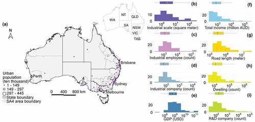
This study investigates eight urban indicators and demonstrates the scaling properties of SUAs from the perspectives of industrial development, economy, infrastructure, and innovation. Industrial features include industrial scale, industrial employee, and industrial company. The industrial-scale indicator refers to the total area of industrial regions within each city that support industrial activities of mining, manufacturing, utility supply and waste services. Industrial regions are defined to be large enough to be functional areas. To study economic development in cities, our research investigates total estimated GDP value and total income as urban economic indicators. Our study further analyzes road length and dwelling count as infrastructure indicators. The innovation indicator is measured by the total number of companies providing professional, scientific, and technical services under the scope of the Australian industry. These companies contribute research outputs and development to society, and they are thereafter noted as “R&D company.” The study area and statistical distribution of eight urban indicators are visualized in Figure 1.

Figure 1. Study area and statistical distribution of indicators. Significant urban areas in Australia by population (a), and statistical distribution of urban factors, including industrial scale (b), industrial employee (c), industrial company (d), GDP (e), total income (f), road length (g), dwelling (h), and R&D company (i). Note: WA – Western Australia, SA – South Australia, NT – Northern Territory, TAS – Tasmania, VIC – Victoria, NSW – New South Wales, QLD – Queensland, and SA4 – Statistical Area Level 4 (sub-state boundaries).

The industrial scale is represented by the area of industrial regions. As there is no prepared data representing industrial regions, our study identifies these areas from raw data provided by OpenStreetMap (OSM) and National Pollutant Inventory (NPI). This study defines industrial regions as industrial areas supporting mining, manufacturing, utility supply, and waste services. Our research pre-processed OSM land use data and identified dense infrastructure areas based on POIs. The identified industrial regions are composed of large industrial land use and dense industrial infrastructure areas. The industrial region identification process is based on the Australian Statistical Geography Standards (ASGS) and a POI-based interested spatial region identification workflow (Song et al. 2018). Details of the industrial region identification process are explained as follows. Industrial land use data from OSM are coarse and extremely small areas should be filtered. According to the ASGS, 5000 square meters is the minimal scale of a region with at least one functional infrastructure, and therefore industrial land uses smaller than 5000 square meters are filtered and then considered industrial POIs. Then, 3977 industrial POIs, including converted POIs from land use and spatial points representing infrastructures, from OSM and NPI are processed by the kernel density estimation (KDE) to generate high-density industrial infrastructure areas. The KDE method is executed with 1000 m as a searching radius, 194 m × 194 m (i.e. the median size of the mesh block, which is the finest spatial granularity of ASGS products) as the pixel size for the Epanechnikov kernel (Zhang, Song, and Wu 2022). The 1000-m searching radius refers to the minimal level of the square root of the Statistical Area Level 2 (SA2) functional area. Next, the high-density industrial infrastructure areas are determined by the change of cumulative distribution function (CDF) from KDE with a threshold value of 0.5%. Finally, large industrial land use and dense industrial infrastructure areas are merged, and aggregated industrial areas smaller than 0.49 square kilometers (i.e. the minimal scale of SA2 functional areas in 2016) are filtered.

Urban indicators, data descriptions, and sources are shown in Table 1. All datasets are accessed from OpenStreetMap (OSM), National Pollutant Inventory (NPI), ABS, and Dryad. OSM provides raw datasets including industrial land use and point of interests (POIs) for industrial region identification, and spatial data of nationwide Australian roads (Geofabrik and OpenStreetMap contributors 2021). NPI provides supplementary spatial information on industrial region identification POIs, and these POIs are recorded facilities supporting industrial activities from the Australian government (Department of the Environment and Energy, Australian Government 2016). The ABS census data provide a collection of urban indicators, covering industrial employees and companies, total income, dwelling, and R&D companies (Australian Bureau of Statistics 2020). Finally, the GDP estimation, with USD as a unit, is available from the Dryad platform provided by a research team from Aalto University (Matti, Maija, and Joseph 2020). As an explanatory variable of urban scaling, the urban population is available from the ABS national census (Australian Bureau of Statistics 2017d). This research uses all datasets representing urban scaling status during the financial year 2015–2016.

Table 1. A summary of urban-scaling indicators.

Urban indicator	Unit	Data description	Source
Industrial scale	${\mathrm{m}}^2$	Total key industrial area within cities	OpenStreetMap, National Pollutant Inventory
Industrial employee	Count	Total employees working for key industries within cities	Australian Bureau of Statistics
Industrial company	Count	Total companies registered for key industries within cities	Australian Bureau of Statistics
GDP	USD	Total estimated GDP of cities	Dryad, Aalto University
Total income	AUD (million)	Total reported income of cities	Australian Bureau of Statistics
Road length	Meter	Total road length of cities	OpenStreetMap
Dwelling	Count	Total dwelling within cities	Australian Bureau of Statistics
R&D company	Count	Total companies providing professional, scientific and technical services within cities	Australian Bureau of Statistics

3. Methods

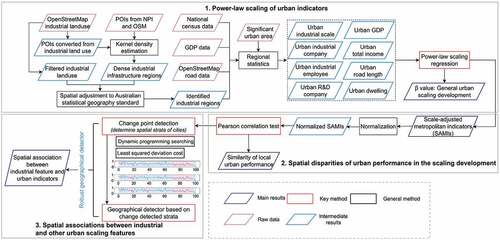
Figure 2 shows the research method workflow, including three main steps. The first step is to compute the power-law scaling of eight urban indicators after industrial region scale identification and urban factor data computation. The second step is to demonstrate the spatial disparity of urban performance in the scaling development, indicated by SAMIs. The last step is to identify the spatial association between industrial features and other urban indicators by analyzing SAMIs using a robust geographical detector.

Figure 2. Flowchart of research methods, including power-law scaling of urban indicators, spatial disparities of urban performance from a scaling perspective, and spatial association between industrial and other scaling features.

3.1 Power-law scaling of urban indicators

3.1.1 Urban indicator data statistics

Eight urban indicators are computed by functions in geographic information systems (GIS). The industrial scale indicator, referring to the total industrial area with cities, is calculated by a “Statistics by categories” method in GIS after all industrial regions are categorized by their belonging cities. ABS provides five urban indicators, including industrial employee and company, total income, dwelling, and R&D company, at the spatial granularity of SA2 level. As cities defined by SUAs are aggregations of SA2 areas (Australian Bureau of Statistics 2017b), these five urban indicators, measured by ABS, are the sum of values recorded by all SA2 areas within cities. The road length indicator is the total length of road lines with cities computed by a “sum line length” function in GIS. The GDP of cities is estimated by the sum of all GDP pixel values within city boundaries using the “Raster layer zonal statistics” method in GIS.

3.1.2 Urban power-law scaling

Cities are developing at the pace of power-law scaling. With the city size represented by urban population, the relationship between the logarithm-transformed urban indicator and logarithm-transformed urban population is linear. The urban power-law scaling relationship is shown in Equation (1)(1) $Y\left(t\right)=\hspace{0.17em}{Y}_0\times P{\left(t\right)}^{\beta }$(1) .

(1) $Y\left(t\right)=\hspace{0.17em}{Y}_0\times P{\left(t\right)}^{\beta }$(1)

where Y(t) refers to the urban indicator; $Y_0$ is a normalization constant; $P\left(t\right)$ is the urban size represented by population; $\beta$ is the scaling exponent indicating urban indicators’ scaling development at a specific time; $t$, which is the year 2016, is the time when these power-law relationships are measured. When urban indicators and urban population are logarithm-transformed, the scaling coefficient values can be calculated via linear regression models.

3.2 Spatial disparities of urban performance in the scaling development

3.2.1 Scale-adjusted metropolitan indicators

Spatial disparities in urban performance, demonstrating characters of each city, are represented by SAMIs (Bettencourt et al. 2010). SAMIs, which are dimensionless and not influenced by city size, are quantified by residuals from urban scaling regressions, shown in Equation (2)(2) ${\epsilon }_i=\mathrm{l}\mathrm{o}\mathrm{g}\left(Y_i\right)-log(Y_0{P}_i^{\beta })=log\frac{Y_i}{Y_0{P}_i^{\beta }}$(2) .

(2) ${\epsilon }_i=\mathrm{l}\mathrm{o}\mathrm{g}\left(Y_i\right)-log(Y_0{P}_i^{\beta })=log\frac{Y_i}{Y_0{P}_i^{\beta }}$(2)

where ${\epsilon }_i$ is the SAMI at city “i;” $Y_i$ is the observed value of the urban indicator at city “i;” $\beta$ is the scaling exponent; $Y_0$ is a normalization constant, and $Y_0{P}_i^{\beta }$ is the estimated value of the urban indicator at city “i.”

In this research, the SAMIs values are interpreted by residual-rank plots to demonstrate the unique properties of each city in urban scaling. Normalized SAMI values can be further analyzed using quantitative models for the relationship between scaling properties. Thus, we use normalized SAMIs in the following spatial analysis processes.

3.2.2 Similarity among cities based on scaling disparities

The similarity among cities is measured by the Pearson correlation coefficient from normalized SAMIs, as shown in Equation (3)(3) $r=\frac{{\sum }_{i=1}^n\left(X_i-\bar{X}\right)\left(Y_i-\bar{Y}\right)}{\sqrt{{\sum }_{i=1}^n{\left(X_i-\bar{X}\right)}^2{\sum }_{i=1}^n{\left(Y_i-\bar{Y}\right)}^2}}$(3) . Similar cities may have common scaling features from industrial development, economy, infrastructure, and innovation perspectives, and the features of each city are represented by normalized SAMIs. In this research, we test the similarity among top-populated cities.

(3) $r=\frac{{\sum }_{i=1}^n\left(X_i-\bar{X}\right)\left(Y_i-\bar{Y}\right)}{\sqrt{{\sum }_{i=1}^n{\left(X_i-\bar{X}\right)}^2{\sum }_{i=1}^n{\left(Y_i-\bar{Y}\right)}^2}}$(3)

where $X_i$ is the i-th normalized SAMI value, representing a kind of scaling feature, of the city X; $\bar{X}$ is the mean value of all normalized SAMI scaling features of the city X; $Y_i$ is the i-th normalized SAMI value of another city Y; $\bar{Y}$ is the mean value of normalized SAMI values of the city Y; n is the number of scaling features, which corresponds to eight urban indicators.

3.3 Spatial analysis on urban scaling disparities – robust geographical detector

Spatial stratified heterogeneity (SSH) is a representation of spatial association based on the fact that the within-strata variance is less than the inter-strata variance (Wang, Zhang, and Fu 2016; Song et al. 2020). The spatial association is determined by spatial strata from the division of the sorted rank of the independent variable. Thus, the SSH value represents how the dependent variable is associated with spatial strata by dividing the rank of the independent variable. The robust geographical detector (RGD) is a measure of SSH value using an optimized discretization algorithm to improve the geographical detector by minimizing the inter-strata variance and increasing the within-strata variance (Zhang, Song, and Wu 2022). The optimization strategy for the RGD model is a change point detection algorithm with a least squared deviation as a cost function and dynamic programming as a searching method. The pseudo code demonstrates how the spatial strata of cities are determined.

Table

	Input: a list of dependant variable values of 101 SUAs sorted by the rank of an independent variable ${\left\{y_x\right\}}_{x=1}^N$, cost function c($y_I$) = $\sum _{x\in I}{\left|\left|y_x-\bar{y}\right|\right|}_2^2$ (least squared deviation), the number of spatial strata K determined by (K-1) change points, number of observations N.
1	for all possible lengths (1 < r < N) of sub-list (p, q) do
2	store the cost value of each sub-list;
3	end for
4	for all the sub-list (p, q) with a length from 2 to K-1
5	find and store the division point that divides sub-list (p, q) into 2 smaller lists with a minimum sum of the cost;
6	end for
7	set the last observation as the first change point; j ← K;
8	while j > 1 do
9	start with the latest change point and find a division point that divides the sub-list into 2 smaller lists with a minimum sum of the cost;
10	store the division point as the latest change point;
11	j ← j − 1;
12	end while
13	return the change point list

The SSH value representing the spatial association between factors can be calculated from the geographical detector after the determination of robust spatial strata of cities. The formula for SSH computation is shown in Equation (4)(4) $B=I-\frac{{\sum }_{h=1}^k{N}_h{\delta }_h^2}{N{\delta }^2}\hspace{0.17em}=I-\frac{SSW}{SST}$(4) (Wang, Zhang, and Fu 2016; Song et al. 2020; Zhang, Song, and Wu 2022). In this research, our RGD model sets the minimum number of observations in each group as no less than five in the optimization algorithm processing. To be consistent with the SAMI-rank analysis, the RGD model uses the descending order rank to determine spatial zones:

(4) $B=I-\frac{{\sum }_{h=1}^k{N}_h{\delta }_h^2}{N{\delta }^2}\hspace{0.17em}=I-\frac{SSW}{SST}$(4)

where $N_h\hspace{0.17em}$is the number of observations within the sub-stratum h by discretizing the explanatory factor; N is the total number of observations; ${\delta }_h^2$ is the variance within a sub-stratum h by discretizing the explanatory factor; ${\delta }^2$ is the variance of the whole study area. SST refers to the Sum of Squares Total and SSW refers to the Sum of Squares Within spatial strata. The B value ranges from 0 to 1. A higher B value indicates a stronger spatial association between two variables. The B value is a measure of spatial stratified heterogeneity, which is also an indicator of the power of determinants. One of the primary research purposes of this study is to identify the spatial relationship between industrial features and other urban indicators based on scaling properties. The response variable is the normalized SAMI value from one of the industrial feature indicators, and the explanatory variable is the normalized SAMI value from one of the urban indicators under the category of economy, infrastructure, and innovation. All 101 SUAs are divided into multiple strata based on the rank of an explanatory variable using RGD.

4. Results

4.1 Power-law scaling of urban indicators

The average scaling development of eight urban indicators from four categories is measured based on urban scaling regressions, and statistical results are demonstrated in Figure 3 and Table 2. According to urban scaling coefficients and their 95% CI value range, scaling paces of industrial scale and infrastructure indicators are sub-linear, scaling paces of industrial employee development and industrial company development are almost linear, and power-law developments of economy and innovation indicators are super-linear. All urban scaling regression models are robust with adjusted R-squared values no less than 0.7 and all p-values for F-statistics are significant at the 0.01 level. The general results, which show the sigmoidal development of infrastructure scaling indicators and booming development of wealth and innovation, coincide with general findings and assumptions of the urban scaling theory. It is worth noting that this study differentiates the computation of industrial scale and other urban indicators. As the industrial scale considers regions large enough to be functional areas only, not every city has one or more industrial regions inside. There are 50 large cities that have industrial regions inside. Therefore, when analyzing the industrial scale indicator in urban scaling regression and further spatial or aspatial relationships involving this factor, computation results are based on these 50 observations with industrial regions.

Figure 3. Urban scaling regression results. (a) Urban scaling of industrial features. (b) Urban scaling of economic indicators. (c) Urban scaling of infrastructure indicators. (d) Urban scaling of the innovation indicator.

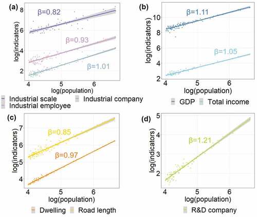
Table 2. Urban scaling of industrial features, economy, infrastructure, and innovation.

Urban indicator	β value	95% CI	Adj-${\mathrm{R}}^2$	Category
Industrial scale	0.82	[0.67, 0.97]	0.70	Industrial feature
Industrial employee	0.93	[0.86, 1.00]	0.88	Industrial feature
Industrial company	1.01	[0.97, 1.06]	0.95	Industrial feature
GDP	1.11	[1.03, 1.18]	0.90	Economy
Total income	1.05	[1.01, 1.09]	0.97	Economy
Road length	0.85	[0.80, 0.90]	0.93	Infrastructure
Dwelling	0.97	[0.96, 0.98]	0.99	Infrastructure
R&D company	1.21	[1.16, 1.26]	0.96	Innovation

4.2 Spatial disparities of urban performance from a scaling perspective

The urban scaling theory suggests a sub-linear scaling development for infrastructure indicators and super-linear development for wealth and innovation indicators. The sub-linear infrastructure scaling development is due to the optimized design and efficiency of the urban system, and this value also implies the share ratio of public facilities for cities. Local infrastructures are publicly shared by residents where the scaling coefficient is low. This fact further indicates that cities with negative SAMI values for infrastructure indicators have higher efficiency in infrastructure design than the average level. On the contrary, wealth and innovation are developing at an accelerating speed and high scaling coefficients indicate relatively fast developments. Therefore, cities with positive SAMI values for wealth and innovation indicators have greater development potential than the average level of the whole system.

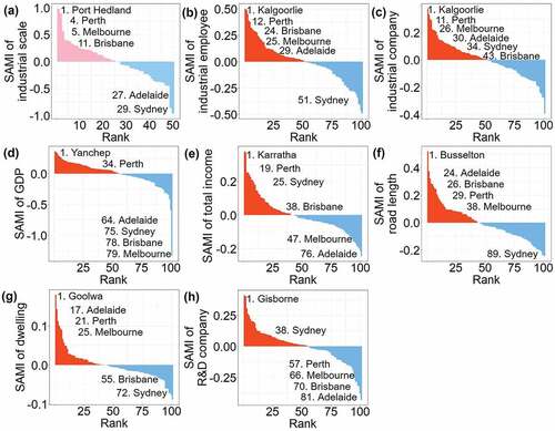
Thus, apart from general scaling development indicated by scaling coefficients, the character of each city indicated by SAMIs can also provide valuable information. Statistical distributions of SAMIs of eight urban indicators are further analyzed by their rank as shown in Figure 4. The top-ranked city of each scaling relationship and five Australian major capital cities are highlighted in these figures. According to SAMI-rank plots, Sydney surpasses the other four major cities in terms of scaling performance in infrastructure efficiency, economy, and innovation. Figures 4(a), Figure 4(F), and Figure 4(g) demonstrate that Sydney has negative SAMI values for industrial region scale, road, and dwelling. These facts indicate that the infrastructure design in Sydney is relatively efficient from the view of urban scaling. Sydney has higher SAMI values in both total income and R&D company as shown in Figures 4(e) and 4(h), which further implies Sydney’s higher accelerating achievement in economic and innovation than the average level. Two economic SAMIs from Figures 4(d) and 4(e) also suggest that Perth has a good economic performance in urban scaling. Top-ranked cities according to SAMIs performance, including industrial design, infrastructure and economic development, and innovation, have no bias on the population size. This fact is consistent with the scale-independent assumption in the scaling theory (Bettencourt et al. 2010).

Figure 4. SAMI-rank plots. SAMIs rank of urban indicators, including (a) industrial scale, (b) industrial employee, (c) industrial company, (d) GDP, (e) total income, (f) road length, (g) dwelling, and (h) R&D company.

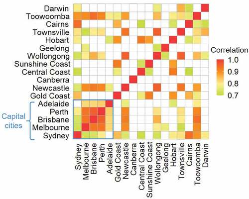
The similarity among large cities measured by eight urban indicators is summarized in Figure 5. The top four populated cities (i.e. Sydney, Melbourne, Brisbane, and Perth) are similar in eight urban scaling features. Scaling characters represented by SAMI values of Melbourne, Brisbane, and Perth are more correlated. The scaling development of Sydney is similar to a majority of top-populated cities to different extents. It is worth noting that the city of Toowoomba is also similar to cities with top-ranked residents from the view of scaling development.

Figure 5. Similarity among Australian major cities assessed by normalized SAMIs. Note: Cities are sorted by the resident population. The white pixel in the correlation matrix indicates no statistically significant results.

4.3 Spatial association among urban scaling disparities

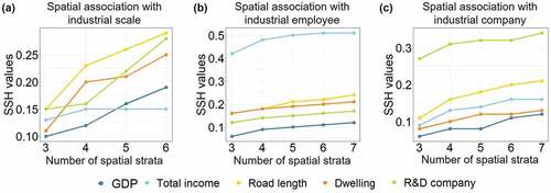
The spatial association between industrial features and urban indicators from other categories is analyzed by the RGD model, shown in Figure 6. According to a pilot study of the robust geographical detector, it is accurate to test the predominance of associated factors with different numbers of spatial strata prior to a conclusion (Zhang, Song, and Wu 2022). Thus, in this study, the spatial association between industrial features and other urban indicators is demonstrated from multiple tests with an increasing number of spatial strata. Infrastructure indicators and the innovation indicator can partially explain the industrial scale of cities from 25% to 29% with the increase of spatial strata as shown in Figure 6(a). However, the difference in the power of determination, for the industrial-scale feature, among indicators is not significant. As shown in Figure 6(b), the urban indicator of total income can significantly explain features of scaling in industrial employees, and the B value increases from 42% to 51% with the increase of spatial strata from three to seven. In other words, the feature of total income can explain around 50% of industrial employee scaling features. The power of explanation of income level is far stronger than the other urban indicators. The feature of scaling in industrial companies is more associated with the innovation feature compared with indicators from other categories, as shown in Figure 6(c). The innovation feature can explain 27% to 34% of the industrial company feature with the increase of the number of spatial strata, and the power of determination of innovation is much greater than that of road infrastructure, ranking second, from 11% to 21%. The geographical-detector-based model can imply spatial association among factors according to the power of determinants (i.e. SSH values), and how pre-dominant variables are associated with industrial scaling features can be further inferred from the spatial and statistical distribution of response variable observations by strata determined by explanatory variables.

Figure 6. The value of industrial features spatially associated with economy, infrastructure, and innovation factors, from the view of urban power-law scaling rule, with the increase of the number of spatial strata. (a) Industrial scale’s association with other indicators. (b) Industrial employee’s association with other indicators. (c) Industrial company’s association with other indicators.

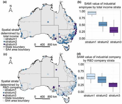
The industrial features associated with the predominant urban factors are assessed by the robust geographical detector, while how these features are spatially associated remains to be explored. Figure 7 provides a supplementary spatial explanation of the results shown in Figure 6. Figure 7 further demonstrates how the industrial employee is associated with the total income feature, and how the industrial company scaling feature is associated with the R&D company feature in cities. The spatial pattern of strata from industrial employees and industrial companies determined by their pre-dominant factors at the strata number of three is shown in Figure 7 to draw the conclusion, as the predominance of associated factors does not change with the increase of strata. The association between industrial employees and total income, and that between the industrial company and R&D company are both statistically significant at the strata of three. This study uses the descending order rank to determine spatial zones from RGD and be in line with the SAMI-rank analysis. Thus, take the association between industrial employees and total income as an example, “stratum1” is the group determined by observations with the top-ranked normalized total income SAMI, and “stratum3” is composed of the bottom-ranked normalized total income SAMI values. As shown in Figure 7(a), the top income SAMI group observations are distributed in remote areas of Australia, and the median group contains a majority of cities including Sydney, Melbourne, and Perth. Figure 7(b) indicates a general positive association between industrial employees and total income, as the average level of industrial employees SAMI drops with the decrease of total income SAMI values. How scaling feature of industrial company is associated with R&D company is demonstrated in Figures 7(c) and 7(d). As shown in Figure 7(c), the top R&D company SAMI group includes Sydney, Melbourne, Brisbane, and Perth. This also implies that the synergy between industrial companies growth and innovation development in major capital cities is evident. The median group is located close to the coast of the Australia continent, and the bottom group is distributed in South Australia and the inner continent. Figure 7(d) also indicates a relative positive association between the industrial company feature and the R&D company feature. The average level of industrial company SAMI value decreases from the top-ranked group to the bottom-ranked group.

Figure 7. Spatial strata of industrial features by predominant influential factors. (a). Spatial strata of industrial employee by total income. (b). Statistical distribution of normalized SAMI value of industrial employee by spatial strata of total income. (c). Spatial strata of industrial company by R&D company. (d). Statistical distribution of normalized SAMI value of industrial company by spatial strata of R&D company.

5. Discussion

This research identified the scaling development of eight urban features from industrial development, economy, infrastructure, and innovation perspectives. Properties and disparities of each city in scaling pace were indicated by SAMIs. Considering the importance and contribution of mining, manufacturing, utility supply, and waste services, we further analyzed the spatial association between industrial features and urban indicators from other categories. Through a series of computation processes, this research identified the paces of scaling achievement for Australian cities using urban scaling models, and the scaling coefficients coincide with scaling theory assumptions. This research also validates the scale independence of power-law scaling characters. Top-performance cities according to SAMIs are not related to the urban size, and this is consistent with the scaling assumptions (Bettencourt et al. 2010). Despite population size independence in scaling disparity, the urban performance of major capital cities is similar from an urban scaling perspective. Furthermore, among these top populated cities, Sydney has a good scaling development in economy, infrastructure, and innovation. Finally, results from RGD show that industrial employee is highly and positively associated with income level, and the industrial company is also positively associated with R&D company. The synergy between industrial companies growth and innovation development in major capital cities is evident.

In terms of the methodological design, this research analyzes scaling properties in Australian cities by fully investigating open-access socioeconomic data from OSM and Australian census data. Apart from traditional statistical analysis on scaling coefficients and SAMIs, we further applied an advanced spatial association analysis method to figure out the pre-dominant indicator of industrial features. Spatial features of urban scaling have long been a key topic in urban studies, and this research explores spatial relationships among scaling indicators using an improved geographical detector algorithm.

This is a cross-sectional research in urban scaling, and research efforts in the future can make the work toward a temporal study. The Australian government is conducting an inclusive national census survey every five years, and both spatial and statistical datasets representing the same urban indicators are updated twice a decade. Therefore, in the future, Australian cities’ scaling development in the post-pandemic era can be further analyzed when national census data are processed and fully open to the public.

This research is a pilot investigation on spatial association among urban scaling features, and future research can be implemented and enriched by various spatial methods and data. From a methodology design perspective, our study demonstrates the spatial association between industrial scaling features and other urban characters. In contrast, the interactive influences of multiple urban factors on industrial features remain to be explored. The development of urban systems is dynamic and synergistic, and thus the economy, infrastructure, and innovation factors may impose an interactive impact on industrial size change. Therefore, the interactive detector of “Geodetector” and its advanced models can be applied to urban scaling studies in future work. From a data enrichment perspective, this research is supported by free open-access data sources including OpenStreetMap and ABS. More urban factors for Australian cities can be accessed from cloud-based public spatial data platforms, including Google Earth Engine and Australian Urban Research Infrastructure Network, in the future.

6. Conclusion

Urban features are developing at the pace of power-law scaling. Spatial effects in the scaling characters of cities are evident, while spatial association among multiple urban features remains to be explored. Industrial features are one of the most important characteristics of urban development, and these features deserve more research efforts. Considering current gaps in investigating association among urban scaling features and limited knowledge on the power-law scaling of Australian cities especially the industrial performance, this study aims to identify spatial disparity of urban performance from a power-law scaling perspective in Australia and explore the spatial association between industrial features and other urban indicators. We use power-law models to assess the scaling development of urban indicators and disparities of urban performance, and RGD models to explore the spatial association between industrial features and other urban indicators. This study validates the general consistency of the scaling development among Australian cities with the power-law theory and the similarity of scaling disparity features among top-populated cities. Spatial analysis results show that the urban innovation indicator and the income level are predominantly and positively associated factors with industrial companies and employees, indicating that the innovation growth and economic development in Australian cities would stimulate the performance of industrial companies and the employment scale. The robust geographical detector categorizes major capital cities into a stratum with high industrial company performance corresponding to high innovation growth, indicating that the synergy between urban innovation and industrial company performance is especially significant in large capital cities. This study explores further spatial properties of urban performances from a power-law scaling perspective and reveals the pace of development in Australian cities, especially industrial features. Future research efforts on census data released at different periods can enrich current cross-sectional results toward temporal outcomes.

Disclosure statement

No potential conflict of interest was reported by the author(s).

Data availability statement

The data and codes that support the findings of this study are openly available in [figshare] at [https://doi.org/10.6084/m9.figshare.21064123].

References

- Australian Bureau of Statistics. (2017a). Australian Industry. [Data set]. Retrieved from https://www.abs.gov.au/AUSSTATS/[email protected]/DetailsPage/8155.02015-16?OpenDocument
- Australian Bureau of Statistics. (2017b). Australian Statistical Geography Standard (ASGS): Volume 1- Main Structure and Greater Capital City Statistical Areas, July 2016. [ Data set]. Retrieved from https://www.abs.gov.au/AUSSTATS/[email protected]/DetailsPage/1270.0.55.001July%202016?OpenDocument
- Australian Bureau of Statistics. (2017c). Australian Statistical Geography Standard (ASGS): Volume 4 - Significant Urban Areas, Urban Centres and Localities, Section of State. [ Data set]. Retrieved from https://www.abs.gov.au/AUSSTATS/[email protected]/DetailsPage/1270.0.55.004July%202016?OpenDocument
- Australian Bureau of Statistics. (2017d). Census of Population and Housing: Mesh Block Counts, Australia. [Data set]. Retrieved from https://www.abs.gov.au/ausstats/[email protected]/mf/2074.0
- Australian Bureau of Statistics. (2020). Data by Region, 2014-19. [Data set]. Retrieved from https://www.abs.gov.au/AUSSTATS/[email protected]/DetailsPage/1410.02014-19?OpenDocument
- Bettencourt, L. M. A. 2013. “The Origins of Scaling in Cities.” Science (New York, NY) 340 (6139): 1438–13. doi:10.1126/science.1235823.
- Bettencourt, L. M. A., J. Lobo, D. Helbing, C. Kühnert, and G. B. West. 2007. “Growth, Innovation, Scaling, and the Pace of Life in Cities.” Proceedings of the National Academy of Sciences of the United States of America 104 (17): 7301–7306. doi:10.1073/pnas.0610172104.
- Bettencourt, L. M. A., J. Lobo, D. Strumsky, and G. B. West. 2010. “Urban Scaling and Its Deviations: Revealing the Structure of Wealth, Innovation and Crime Across Cities.” Plos One 5 (11): e13541. doi:10.1371/journal.pone.0013541.
- Bettencourt, L. M. A., V. C. Yang, J. Lobo, C. P. Kempes, D. Rybski, and M. J. Hamilton. 2020. “The Interpretation of Urban Scaling Analysis in Time.” Journal of the Royal Society Interface 17 (163): 20190846. doi:10.1098/rsif.2019.0846.
- Department of the Environment and Energy, Australian Government. (2016). National Pollutant Inventory. [Data set]. Retrieved from http://www.npi.gov.au/npidata/action/load/browse-search/criteria/browse-type/Industry/year/2016
- Geofabrik and OpenStreetMap contributors. (2021). Download OpenStreetmap for This Region: Australia and Oceania. [Data set]. Retrieved from http://download.geofabrik.de/australia-oceania.html
- Keuschnigg, M., S. Mutgan, and P. Hedström. 2019. “Urban Scaling and the Regional Divide.” Science Advances 5 (1): eaav0042. doi:10.1126/sciadv.aav0042.
- Khan, F., and L. Pinter. 2016. “Scaling Indicator and Planning Plane: An Indicator and a Visual Tool for Exploring the Relationship Between Urban Form, Energy Efficiency and Carbon Emissions.” Ecological indicators 67: 183–192. doi:10.1016/j.ecolind.2016.02.046.
- Kozlov, A., S. Gutman, I. Zaychenko, and E. Rytova (2017). The Formation of Regional Strategy of Innovation-Industrial Development. In Information Systems Architecture and Technology: Proceedings of 37th International Conference on Information Systems Architecture and Technology – ISAT 2016 – Part IV (pp. 115–126). Karpacz, Poland: Springer International Publishing.
- Kwon, O. 2018. “Scaling Laws Between Population and a Public Transportation System of Urban Buses.” Physica A: Statistical Mechanics and Its Applications 503: 209–214. doi:10.1016/j.physa.2018.02.193.
- Lämmer, S., B. Gehlsen, and D. Helbing. 2006. “Scaling Laws in the Spatial Structure of Urban Road Networks.” Physica A: Statistical Mechanics and Its Applications 363 (1): 89–95. doi:10.1016/j.physa.2006.01.051.
- Lei, W., L. Jiao, and G. Xu. 2022. “Understanding the Urban Scaling of Urban Land with an Internal Structure View to Characterize China’s Urbanization.” Land Use Policy 112 (105781): 105781. doi:10.1016/j.landusepol.2021.105781.
- Lei, W., L. Jiao, G. Xu, and Z. Zhou. 2022. “Urban Scaling in Rapidly Urbanising China.” Urban Studies (Edinburgh, Scotland) 59 (9): 1889–1908. doi:10.1177/00420980211017817.
- Lobo, J., L. M. A. Bettencourt, D. Strumsky, and G. B. West. 2013. “Urban Scaling and the Production Function for Cities.” Plos One 8 (3): e58407. doi:10.1371/journal.pone.0058407.
- Lobo, J., D. Strumsky, and J. Rothwell. 2013. “Scaling of Patenting with Urban Population Size: Evidence from Global Metropolitan Areas.” Scientometrics 96 (3): 819–828. doi:10.1007/s11192-013-0970-3.
- Matti, K., T. Maija, and G. Joseph (2020) Data From: Gridded Global Datasets for Gross Domestic Product and Human Development Index Over 1990-2015. [Data set]. Retrieved from https://datadryad.org/stash/dataset/doi:10.5061/dryad.dk1j0
- Ma, Q., J. Wu, C. He, and G. Hu. 2018. “Spatial Scaling of Urban Impervious Surfaces Across Evolving Landscapes: From Cities to Urban Regions.” Landscape and Urban Planning 175: 50–61. doi:10.1016/j.landurbplan.2018.03.010.
- Ovando-Montejo, G. A., P. Kedron, and A. E. Frazier. 2021. “Relationship Between Urban Size and Configuration: Scaling Evidence from a Hierarchical System in Mexico.” Applied Geography (Sevenoaks, England) 132 (102462): 102462. doi:10.1016/j.apgeog.2021.102462.
- Riascos, A. P. 2017. “Universal Scaling of the Distribution of Land in Urban Areas.” Physical Review E 96 (3–1): 032302. doi:10.1103/PhysRevE.96.032302.
- Rietveld, R., N. Vlaanderen, D. Kame, and Y. Schipper. 1994. “Infrastructure and Industrial Development: The Case of Central Java.” Bulletin of Indonesian Economic Studies 30 (2): 119–132. doi:10.1080/00074919412331336617.
- Sarkar, S. 2019. “Urban Scaling and the Geographic Concentration of Inequalities by City Size.” Environment and Planning B: Urban Analytics and City Science 46 (9): 1627–1644. doi:10.1177/2399808318766070.
- Sarkar, S., P. Phibbs, R. Simpson, and S. Wasnik. 2018. “The Scaling of Income Distribution in Australia: Possible Relationships Between Urban Allometry, City Size, and Economic Inequality.” Environment and Planning B: Urban Analytics and City Science 45 (4): 603–622. doi:10.1177/0265813516676488.
- Song, Y. 2022a. “Geographically Optimal Similarity.” Mathematical Geosciences 8: 1–26. doi:10.1007/s11004-022-10036-8.
- Song, Y. 2022b. “The Second Dimension of Spatial Association.” International Journal of Applied Earth Observation and Geoinformation 111: 102834. doi:10.1016/j.jag.2022.102834.
- Song, Y., Y. Long, P. Wu, and X. Wang. 2018. “Are All Cities with Similar Urban Form or Not? Redefining Cities with Ubiquitous Points of Interest and Evaluating Them with Indicators at City and Block Levels in China.” Geographical Information Systems 32 (12): 2447–2476. doi:10.1080/13658816.2018.1511793.
- Song, Y., J. Wang, Y. Ge, and C. Xu. 2020. “An Optimal Parameters-Based Geographical Detector Model Enhances Geographic Characteristics of Explanatory Variables for Spatial Heterogeneity Analysis: Cases with Different Types of Spatial Data.” GIScience & Remote Sensing 57 (5): 593–610. doi:10.1080/15481603.2020.1760434.
- Wang, Y., Y. Ding, and L. Yan (2020). Analysis on the Association of Financial Development, Industrial Structure Optimization and Economic Growth via Panel VAR. Proceedings of the 2020 3rd International Conference on E-Business, Information Management and Computer Science, Wuhan, China.
- Wang, J. -F., T. -L. Zhang, and B. -J. Fu. 2016. “A Measure of Spatial Stratified Heterogeneity.” Ecological indicators 67: 250–256. doi:10.1016/j.ecolind.2016.02.052.
- Xiao, Y., and P. Gong. 2022. “Removing Spatial Autocorrelation in Urban Scaling Analysis.” Cities (London, England) 124 (103600): 103600. doi:10.1016/j.cities.2022.103600.
- Xu, G., Z. Xu, Y. Gu, W. Lei, Y. Pan, J. Liu, and L. Jiao. 2020. “Scaling Laws in Intra-Urban Systems and Over Time at the District Level in Shanghai, China.” Physica A: Statistical Mechanics and Its Applications 560 (125162): 125162. doi:10.1016/j.physa.2020.125162.
- Yang, C., and S. Zhao. 2023. “Scaling of Chinese Urban CO2 Emissions and Multiple Dimensions of City Size.” The Science of the Total Environment 857 (Pt 2): 159502. doi:10.1016/j.scitotenv.2022.159502.
- Zhang, Z., Y. Song, and P. Wu. 2022. “Robust Geographical Detector.” International Journal of Applied Earth Observation and Geoinformation: ITC Journal 109 (102782): 102782. doi:10.1016/j.jag.2022.102782.