
 ?Mathematical formulae have been encoded as MathML and are displayed in this HTML version using MathJax in order to improve their display. Uncheck the box to turn MathJax off. This feature requires Javascript. Click on a formula to zoom.
ABSTRACT
The Voronoi diagram (VD) is a fundamental geo-computing structure that has crucial applications. Computing this structure on a topographic surface requires having every point clustered on the geodesic distances, and thus the same challenging task as the geodesic distance mapping. This article proposes a new algorithm for the geodesic VD (GVD) by breaking up the highly complicated task into regular routines on the exact computation. The exact approach is due to the irregular rough nature of the Earth surface, where the discrete computation is more appropriate. The key operation involves a direct window growth devised to avoid the overloaded facet splitting and realized in a conic arrangement. Conventional clustering and GVD structure post-extraction are built on top of the window growth. The fundamental role of GVD in geo-computing is then demonstrated. The experimental results showed that the dual structure of GVD is useful in justifying the potential wrong triangulations from the popularly used 2D Delaunay, and the geometric exactness of GVD is more reliable in guaranteeing the surface process model efficiency and convergence, under the harsh checking of centroidal Voronoi tessellation optimization.
1 Introduction
The Voronoi diagram is a fundamental structure in geo-computing. However, computing this structure on a topographic surface is still challenging (Aronov, Berg, and Thite Citation2008; Liu Citation2018). As a result, classical planar VD applications cannot be rigorously replanted. For example, the Delaunay triangulation from the dual operation of VD on topography is not feasible yet, whereas existing 2D Delaunay triangulation works on projecting and raising of the 2D grid (Cheng, Dey, and Shewchuk Citation2012). The VD structure often acts as the spatial discretization in surface process simulations (Okabe et al. Citation2000). In the long run of the model integral, repeated geometric errors from the underlying spatial unit had been reported contributing to considerable model uncertainty (for example, Elvidge et al. Citation2019).
Computing the VD on topography amounts to clustering every point to the nearest sources (seeds/generators) along the surface. This requires a geodesic distance mapped on the surface, especially, a multiple source geodesic mapped, for extraction of the geodesic VD (Papadopoulou and Lee Citation1998). Supposing that there is a set of heat sources site on the topography, the geodesic mapping can be analogous to heat diffusion that evolves along the shortest paths to cover the entire surface. PDE-based (partial differential equations) methods numerically simulate the evolution with concise discretization schemes that are sophisticated in the scientific computing community. Since they are built upon continuous heat flow physics, they are suitable for smooth settings and produce smoothed geodesics (see for more explanation). Mainstream approaches, such as the fast marching method (Kimmel and Sethian Citation1998) and the heat method (Crane, Weischedel, and Wardetzky Citation2013), involve direct solvers of a sparse linear system, and thus may not apply to large meshes due to the memory limit, while the restored sparse geodesics along vertices have only first-order accuracy and may not satisfy the metric requirement (Crane et al. Citation2020).
Figure 1. A surface grid and a standard Laplacian discretization of the PDE methods. The Laplace-cotan operator is formulated as , where
is the heat value at vertex
,
is the one-third area of the triangles incident to vertex
, from Bobenko and Springborn (Citation2007). Notably, whatever how delicate the operators are, they are approximations of the continuous heat derivatives in time and space, whereas the underlying Earth surface is rather rough than smooth.
Computational geometry-based methods organize window propagation to simulate the heat diffusion waves in discrete settings. Windows are visibility wedges on facet edges that have shortest paths to the source; this is further explained in Section 2.1. The windows implicitly split the surface mesh into continuous, slim cones with exact geodesics, but are known as slow for the overloaded window bifurcation and window pruning caused by the irregular surface bumps (Crane et al. Citation2020; Liu, Chen, and Tang Citation2011). presents a simple demonstration.
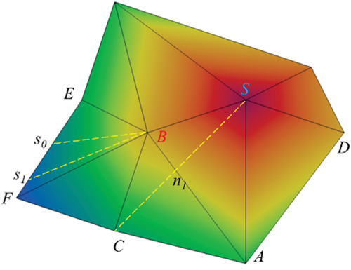
Figure 2. Computational geometry methods organize the geodesic wave propagation in linearly truncated windows. five windows (i.e. waves) emanated from the source S in the first propagation. The wave was back-pruned as
and
in the following propagation. vertex B was an obstacle point where the wave was bifurcated into three parts. For the invisible to source part of
,the propagation was not stopped but relayed by vertex B. The dotted lines show a portion of the implicit splitting. The red-to-blue color indicates the distance increase.
Since a discrete mesh can also be regarded as a graph, efficient graph search algorithms can be exploited to avoid the window bifurcations and prunes (Bose et al. Citation2011; Lanthier Citation1999). The graph-based methods work on excess a prior mesh splitting, but the geodesics accuracy is approximated (). For example, the Dijkstra distance along the facet edges will obviously overestimate the true geodesics. Recent works, such as the saddle vertex graph and the proximity graph, stressed the separation of the distance query and set up by taking designated and delicate a prior splitting, which is very fast (in the query phase) with accuracy improved (Adikusuma, Fang, and He Citation2020; Wang et al. Citation2017; Xin et al. Citation2018). However, if the accuracy is sensitive, the additional mesh splitting may become unaffordable. Similar speed-ups by separating the query and set up are also developed in PDE-based methods, where matrix pre-factorization and back-substitution, along with localized solvers (Herholz and Alexa Citation2018; Nazzaro, Puppo, and Pellacini Citation2021) drive the super-fast efficiency and greatly improve the scalability.
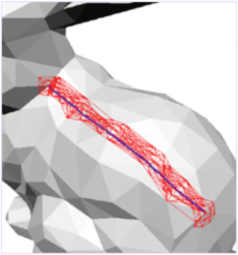
Figure 3. Excess a prior mesh splitting (the grids in red) for approximating the geodesic (the solid curve in blue) of graph-based methods, from Kanai and Suzuki (Citation2001). Because there is no exact information for reference, the geodesic is searched and approximated from the excess paths. More delicate pre-computations for graph-based geodesics are referred to Ying, Wang, and He (Citation2013) and Xin et al. (Citation2018).
Meanwhile, computational geometry-based methods have also made substantial progress, on improving the seminar MMP (Mitchell, Mount, and Papadimitriou) framework (Mitchell, Mount, and Papadimitriou Citation1987; Surazhsky et al. Citation2005) of window propagation, window pruning, and window management. The CH (Chen and Han) algorithm removes window redundancy around vertices, and proposes a FIFO (first in first out) queue instead of the MMP’s priority queue (Chen and Han Citation1990). It opens a door for parallel propagation (Xiang, Xin, and Ying Citation2014) and window pruning reduction. ICH (improved CH) filters redundant window by distances around vertices while re-integrating the priority queue (Xin and Wang Citation2009). FWP (fast frontwave propagation) uses window buckets of similar distances for propagation (Xu et al. Citation2015), and VTP (vertex-oriented triangle propagation) manages the propagation triangle-wise, the consideration of distances and geometric interrelationships as well makes VTP a state-of-the-art method of discrete computation (Qin et al. Citation2016). In summary, VTP provides comparable efficiency to graph methods with less memory consumption in terms of exact computation.
Although geodesic mapping is mature in applications, computing the GVD is still challenging (Liu Citation2018). On the boundary facets where geodesics from different sources meet, PDE methods provide no information on the exact bisectors (which comprise the GVD edge arcs) that separate the different sources, for they focus on solving the sparse distances on a smoothed-out domain. Computational geometry methods record analytical bi-sectioning information during the geodesic propagation, but the wave fronts are always encoded in a linear window structure. More specifically, computational geometry methods store lateral characteristics that bi-section the direct-adjacent windows, but the front hyperbolic bisectors are circumvented with the linear windows. The bisectors are generally hyperbolic arcs; more details are given in Section 2.2.
To compute GVD with exact boundaries, the geodesic distance mapping is needed to cover the boundary facets with the bisector information exposed. Skills such as splitting and localized refinement are favored again for this approximation. Thus, the process is as complicated as the geodesic mapping, albeit with a smaller scale (boundary facets usually take a minority amount of the mesh facets). Some researchers have clustered the mesh facets to get the so-called grid-GVD or raster-GVD (Chen Citation1999; Stewart and Ree Citation2010), and some other researchers have given up a strict line-style GVD edge (Sharp, Soliman, and Crane Citation2019) or taken a band-style GVD boundary (Zayer et al. Citation2018). PDE methods often adopt iterative splitting with linear interpolation to produce a well-approximated GVD (Herholz, Haase, and Alexa Citation2017). Computational geometry methods often recursively split the boundary facets into simpler triangles containing windows with at most three different sources, where Liu, Chen, and Tang (Citation2011) describe a propagation integrated exact GVD algorithm. Afterward, Xu et al. (Citation2015) reported the polyline-sourced GVD on the window propagation, and Qin, Yu, and Zhang (Citation2017) reported the VTP-based GVD, on a similar strategy. Since non-boundary facets take a majority amount of the mesh facets, the geodesic mapping time dominates in the GVD algorithms, these reports focus more on revising the window propagation efficiency than the GVD extraction.
It is natural to derive the GVD algorithm through geodesic mapping extension. However, this method demands all the high skills of the distance mapping framework, and the integrated algorithms are too complicated for common GIS investigations.
In this article, the GVD solution starts from the computed exact geodesics, for which the MMP/VTP methods have laid a concrete basis. One strong support for the exact geodesics is the irregular rough nature in almost all scales of the Earth surface (Smith Citation2014). If the discrete TIN grid (triangulated irregular network) is the optimal representation of a topographic surface, exact geodesics is more suitable than the PDE geodesics (a comparison with realistic datasets is presented in the supplementary materials). Subsequently, the GVD algorithm can exploit the readily exact clues pointing to the GVD edges and vertices, other than finding a PDE approximation step-wisely. In searching a simpler way of GVD algorithm, this article makes three objectives:
A direct window growth is devised to avoid the recursive pre-subdivision. Exact geodesics have made success but have also been criticized for the slow efficiency from the overloaded splitting. In practice, sliver subdivisions often lead to geodesic mapping instability, and we will show typical subdivision examples with numerical handlings in the experiment. The window growth is encapsulated in the form of hyperbolae growth emanated from the two end-points of the window (the pruning-points between windows represent the space equilibrium between the two direct-adjacent sources), a group of criteria for the growth is defined under the elementary 2D conic arrangements; The window growth termination is discussed, at the end, the boundary facet is accurately tessellated, and each tessellated cell is correctly labeled to its source.
A phased algorithm is proposed by resolving the highly complicated GVD generation into regular routines. That is, clustering the non-boundary facets, tessellating the boundary facet by window growth, and clustering of the tessellated cells; The cluster is organized in a triangle soup for simplicity, the GVD structure is post-extracted and thus avoids the dynamic maintenance of a complex global data structure proposed by the literature (the analytic GVD data structure involves edges of hyperbolics and line segments, joined by break points, while break points are essentially not GVD vertices. More details are found in section 2). All the operations are built on consolidated concepts.
Applications of the exact GVD are explored and demonstrated to stress its fundamental role in geo-computing, theoretically and practically. The most frequently questioned application of GVD is the dual operation, where 2D Delaunay triangulation is widely used but works on a non-rigorous background. GVD is used to justify the potential wrong triangulations from the 2D Delaunay. Another frequent GVD application is the space discretization of the surface process simulations, where model integral of material, energy, and momentum is based on the underlying GVD cells. Repeated geometric errors from inexact Voronoi cells will lead to cumulative model bias. Here, the CVT (centroidal Voronoi tessellations) is selected as the special surface model, and GVD is examined for mode performance with comparisons to existing in-exact GVDs.
The remainder of this article is organized as follows. Section 2 presents geodesic concepts and introduces the phased GVD algorithm. Section 3 presents the experiments and discussions. Section 4 provides our conclusions and a brief outlook.
2 Methodology
The new GVD algorithm is based on multiple-source geodesic distance mapping, and the key procedure involves the window growth without a prior subdivision. This section starts with the preliminaries to the geodesic characteristics and ends with the algorithm description.
2.1 Saddle points and the bifurcated geodesic propagation
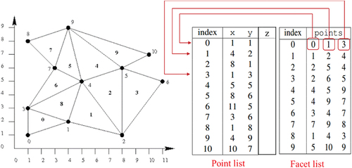
Given a discrete topographic mesh M and a set of source points S on M, M = (V, E, F) is defined in combinatorial topology as the common TIN grid, where V, E, and F are the vertex set, edge set, and facet set, respectively. S is the point set confined to the surface. illustrates the concepts in a simple configuration.
Figure 4. TIN grid M definition in planar space. The point list V defines the geometry, the facet list F defines the topology with indices to V (the edge list E is usually implicit). The combinatorial topology stresses the regularity that each k-cell’s boundary is constrained by the (k-1)-cells. this regularity is strictly required by the MMP/VTP algorithms for propagation convenience, while other algorithms such as the heat method (Sharp et al. Citation2019) may only requires a loose topology as point clouds. The sources are surface points, meaning that they are not confined to mesh vertices or mesh edges (see Fig 11, right).
For any point p on M, geodesic mapping identifies a distance function D(p) that returns the shortest distance between p and one specific source s∈S.
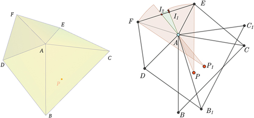
A topographic surface is characterized by irregular bumps. A topographic bump is always accompanied by several saddle points. A saddle point is a vertex with a positive angle defect (the sum of the surrounding angles minus ) which is analogous to the Gauss curvature. Because of this characteristic, the space near the saddle vertex cannot be unfolded onto a single plane. shows such a topographic bump with the saddle sites at vertex A; and on the right of the figure is the unfolded view that shows an un-accommodatable facet ABC.
Figure 5. A topographic bump bifurcates the geodesic wavefront. A saddle point sites at vertex A and a source sites at the surface point P (left). right, the unfolding all facets adjacent to saddle A onto the AEF plane causes source P has two images. denotes the angle defect. The wavefront from source P is bifurcated at saddle A into left and right parts and the relayed part. note that the relayed part has a smaller radius, which indicates the differentiated propagation velocity.
Geodesic distance mapping, as pioneered by the MMP algorithm of computational geometry methods, is primarily based on the following observation (Sharir and Schorr Citation1986): The geodesic is a straight line on the facet; when it crosses the edge, if the adjacent facets are unfolded into the same plane along the common edge, the geodesic will also be a straight line. Similarly, at one moment, the front ends of geodesics from the same source form a circular arc of the geodesic wavefront, unless a saddle vertex or another geodesic wavefront from a different source is encountered.
Geodesic propagates along the shortest path; the topographic bumps delay the propagation at exactly the saddle points. The unfolding view around saddle A in (right) reveals the saddle bifurcation effect. For facet AEF, the straight line crossing source P and saddle A intersects edge EF at I1 and I1, the wavefront from source P covers the AEI1 and AFI2 parts (the fan in light red), while the AI1I2 part (the fan in light green) is invisible to P and the wavefront is relayed by saddle A. Therefore, saddles are called pseudo sources.
The computational geometry methods record the intersection points and encapsulate the line segments EI1, I1I2, and I2F as visibility windows. The visibility windows store key information such as the id, distance, and direction of the sources P and A. With the geodesic wavefronts proceeding, the visibility windows implicitly split the surface mesh into accurate while slim cones.
Notably, the wavefronts are conic arcs, whereas the visibility windows are linear data structures. In other words, the MMP-like algorithms record lateral characteristics rather than the front conic characteristics, of the geodesic distances. This has posed a substantial challenge for the GVD algorithm: on the boundary facets where two or more geodesics from different sources meet to form GVD edges and vertices, the splitting of the facets are stopped and circumvented, and the linear windows are left on the edges.
A boundary facet is a facet whose visibility windows have two or more sources where the GVD structures reside. A non-boundary facet is a facet whose visibility windows have exactly one-identical source.
2.2 Circular wavefronts meet and a hyperbolic bisector grows
In the multiple-source geodesic mapping procedure, the wavefront keeps circular arc propagation until it meets other wavefront and comes to a spatial equilibrium. shows two kinds of meetings: wavefronts from different sources (left) and wavefronts from the identical source (right).
Figure 6. Circular wavefronts meet and spatial competition is equilibrated as singular loci. left: wavefronts from different sources P0 and P1 meet at singularity S00; right: wavefronts from different directions of the same pseudo-sources P1/P2 meet at singularity S01. At a meeting point, a hyperbola can be grown (see light-green dotted curve) for space equilibration on behalf of its left/right windows. note the solid-green directional arcs are truncated by the facet for further use.
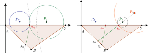
When the wavefronts meet, a singularity forms. A singularity is a point in space with more than two sources. The continuous singular points in space form a singular locus, which is the bisector between two direct-adjacent (pseudo-) sources. The computational geometry methods implicitly record the lateral singular loci (pseudo-bisector) on the non-boundary facets, i.e. meeting loci of wavefronts from the same (pseudo-) sources but different directions. Meeting locus of wavefronts from two distinct sources is called front singular locus.
On the boundary facets, both the front and lateral singular loci are circumvented, while the singularities are recorded as the endpoints of windows. As shown in (left), singularity S00 is the bi-sectioning point that separates windows AS00 (with source P0) and S00C (with source P1). For S00,
where d(P) is the distance to the source and |PS| is the Euclidean distance between points P and S. Because in common, EquationEquation (1)
(1)
(1) represents a hyperbola: the trajectory of a point with a constant distance difference to two fixed points (the foci P0/P1). This hyperbola represents the bisector between the sources P0 and P1.
Therefore, using the three-point (P0, P1, and S00) formulation, a hyperbola can be grown for space competition on behalf of its left/right windows. Starting from S00, the hyperbola should be truncated with facet ABC and be oriented as the directed conic arc . More details on the arc truncation and orientation are provided in the supplementary materials.
The singularity and singular locus are analogous to the vertex and edge concepts in combinatorial topology, i.e. at such locations the connectivity changes. Subsequently, a GVD vertex is the singularity with three or more sources, a GVD edge is the GVD-vertices-trimmed bisector.
2.3 Linear approximation and shape exactness of the GVD edge
We say the distance of EquationEquation (1)
(1)
(1) in the local coordinate system on the boundary facet, where P0/P1 in are essentially pseudo-sources (saddles). The local pseudo-sources notion is reinforced by the observations that a majority amount of the mesh vertices are saddle vertices on a realistic surface (Ying, Wang, and He Citation2013).
The local pseudo-sources fact has the following implications:
If both P0/P1 are source points, then
are the distances to themselves and zero, and EquationEquation (1)
If P1/P2 are pseudo-sources but connected to the same source, the bisector symmetrically separating the left/right sources is still a straight line, demonstrated as S01S10 in (right). In this case, the singularity S01 should be distinguished as break point which reflects the bisector discontinuity distorted by the saddles; break points are generally not GVD vertices.
In most cases, P0/P1 are pseudo-sources with distinct sources and different
shows a steep terrain with six source points, where the trimmed bisector arc exhibits an explicit hyperbolic form (left). The arc lies downstream of a saddle point A (right), separating sources P and S. Generally, these hyperbolic arcs are sampled and linearly discretized using a spline (Xu et al. Citation2015).
Figure 7. Steep terrain (rendered in height) with six sources (white points) and the trimmed bisectors (green arcs). A close view of the hyperbolic arc is drawn on the right and compared to the line segment (white), where M/N are break points, and vertex A (the red point) is the saddle. The terrain data is a fragment of the SRTM DEM (90 m resolution) in the Himalaya mountain region and can be found in the supplementary material.
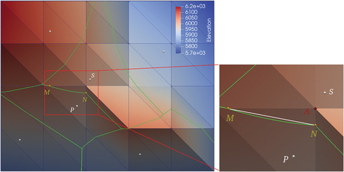
From the close view in (right), it could be observed that the bisector arc is relatively “straight.” We estimate the arc length by , where d is the propagation distance from the pseudo-source, θ is the angle defect at the pseudo-source. Angle defects are usually confined to be no greater than π/2 since the topography is 2.5D, while the propagation distances are easily halved as the mesh is subdivided. With small d and θ values, the shortened conic arcs will appear straighter than the explicit hyperbolae on generic 2-manifold meshes.
In fact, some researchers have proposed using line segments to produce well-approximated GVDs (Herholz, Haase, and Alexa Citation2017). However, it must be noted that a well-approximated linear scheme should preserve the GVD edge shape. At least, the break points (in this case, the M/N points) that represents the GVD edge discontinuities should be retained. Further comparison details are discussed in the experimental section.
The bisectors from edge singularities enter the boundary facets for space competition at different velocity, orders, and directions, forming a wild, challenging conic tessellation (Liu, Chen, and Tang Citation2011). However, each tessellated sub-facet is directly connected to a window on the edge (i.e. no enclave region) (Mitchell, Mount, and Papadimitriou Citation1987). This strong observation guarantees that the tessellated sub-facet is marked correctly with reference to the window’s source, which will help to complete the window growth in the next phase.
2.4 Direct window growth
The growth of a single singular locus completes the equilibrium of the spatial competition of the space direct-adjacent sources. The final spatial competition requires mutual space equilibrium between all source points on the boundary facet. The intersection of newly grown singular loci may form new singular points, representing the space equilibrium between indirectly adjacent source pairs. Therefore, a challenging conic tessellation can be gradually decoupled in a near to far (edge) manner, by repeatedly growing singular loci and generating new singularities around visibility windows.
Remember that the visibility window originally represents the linear truncation of the geodesic wavefront of some distinct (pseudo-)sources and that the endpoint hyperbolic bisectors represent the equilibrated space competition of the direct adjacent sources. Accordingly, window growth is defined by the singular locus growth on a singular point: if the hyperbolic arc growing from two endpoints has an effective near intersection on the boundary facet, the growth of the visibility window is satisfied.
Note that, before the two hyperbolic bisectors grown from the two window endpoints intersect each other, each hyperbolic arc can be intercepted by other existing hyperbolic arcs. The effective near intersection therefore needs to be carefully defined: If the first intersection of the left (or right) hyperbolic arc is also the first intersection of the right (or left) hyperbolic arc, then it is an effective candidate intersection. If the candidate intersection is nearer to the current window source, it is determined to be an effective near intersection. The intersections and the first intersection can be obtained from the arrangement of the x-monotone curves.Footnote1
The decoupling logic organized as singular window growth is then as follows: grow hyperbolic bisectors from the endpoints; check for effective near intersections; create new singularities and update the left and right window information and encapsulate all three steps into a loop check for the availability of new window growth.
After the window growth loop is completed, competitive space claims from all (pseudo-)sources are supported, with the space equilibrated between all direct and indirect adjacent source pairs. The boundary facet is then accurately tessellated, and each sub-facet is properly marked with the connected edge window source, with reference to the key observation of “no enclave region.”
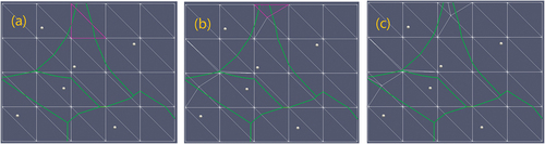
Here, an example of an effective near intersection and singular window growth logic flow is shown in shows six distinct sources (P0–P5) reaching the boundary facet for an exclusive space via six windows on the edges. A pair of directed, singular arcs can be grown from each of the two endpoints of the window (the red singularities S00 and S01 show the beginnings of the arcs). Three candidate intersections (I0–I2) are generated from the windows S10AS00, S01BS21, and S20CS11. Windows S00S01 and S11S10 have no intersection, and the intersection for window S21S20 is intercepted by I1 and I2 and is therefore not an effective intersection. Candidate I0 has no coupling with the other intersections and is an effective intersection. Candidate I1 is the first intersection of the singular locus S21 and the third intersection of the singular locus S01; however, the first two intersections on S01 are not first intersections; therefore, I1 is an effective intersection. Candidate I2 has no coupling with the other intersections but is not nearer to the window source P4; therefore, it is not an effective near intersection either.
Figure 8. Singular grow of the visibility windows from six distinct sources P0–P5. (a) Conic tessellation of singular loci in the first round of growth, where I0–I2 are the three candidate intersections for the new singularities. (b) two new singularities determined at the effective near intersections, with the growth of windows S10AS00 and S01BS21 being satisfied. (c) New singular loci grown from the new singularities. (d) growth of windows S11S10 and S21S20 satisfied. (e) final space equilibrium of the six sources on the boundary facet.
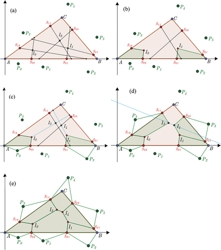
shows the effective near intersections (I0 and I1) generated in a first growth round and the satisfied growth of the visibility windows S10AS00 and S01BS21 (light green areas connected to the sources P0 and P2). shows new singular loci grown on the new singularities (I0 and I1), which are bisectors between the indirectly adjacent source pairs P1 and P3 and P1 and P5 and the new generated candidates (I3 and I4). shows that the growth of the windows S10S11 and S20S21 is satisfied and that the new singular locus (the bisector between the sources P4 and P1) crosses the new singularities (I3 and I4) exactly. shows that the growth of all six windows is satisfied.
2.5 GVD algorithm of clustering, tessellating, and re-clustering
Once the key procedure of direct window growth is finished and the hyperbolic tessellation of the boundary facet is accomplished, a phased GVD algorithm without recursive, overloading subdivision can be completed with conventional operations as facet clustering and GVD structure post-extraction, that is, clustering of the non-boundary facets (, left), tessellating of the boundary facet (, middle), and re-clustering of the hyperbolic-tessellated sub-facets (, right). The overall phased GVD algorithm in pseudo-code is as follows.
Figure 9. Stages of the GVD algorithm. From left to right: non-boundary facet clustering, boundary facet tessellation, and re-clustering of the tessellated sub-facets and the GVD structure extraction.
Algorithm sg_gvd
Input: discrete TIN with n facets, m source points;
Output: TIN tessellated into m GVD cells;
vector L[m]//cluster in source id
vector mk[n];//mark for facet
queue sn;//queue for new visibility windows
(0) geodesic distance mapping with m sources using the MMP algorithm on the TIN grid;
(1) for each facet fk in TIN:
count the number of different sources cnt_src by looping every visibility window;
if cnt_src= = 1: push fk.id into L[ids];//non-boundary facets clustering
else: mk[fk.id]=cnt_src;//boundary facets to be tessellated
(2) for each facet with mk[fk.id]>1:
loop
(2.1) push each visibility window into queue sn; grow 2 singular loci from the window endpoints;
(2.2) for each visibility window VWi, check its effective near end intersection SNx in the conic tessellation;
if found a SNx: create new singularity at the SNx; create new window; update left/right window information; pop VWi from sn;
(2.3) check for new window to be grown;
(2.4) mark the tessellated sub-facets according to the connected edge window sources;
(3) cluster newly tessellated sub-facets; extract GVD structure.
Procedure (0) completes the exact geodesic distance mapping. Procedure (1) completes the non-boundary facet clustering and boundary facet marking. Note that this procedure traverses all window sources to determine the boundary and non-boundary facets because the geodesic on the edge is basically non-linear. Procedure (2) completes the singular window growth described in Subsection 2.4. Procedure (3) completes the re-clustering and the GVD extraction.
In practice, the exact geodesic can be computed using the MMP algorithm (Surazhsky et al. Citation2005) and the VTP algorithm (Qin et al. Citation2016). The only complex data structure used in the new GVD algorithm is the visibility window described by Surazhsky et al. (Citation2005) and Liu, Chen, and Tang (Citation2011). The more complexed GVD analytic structure described by Liu, Chen, and Tang (Citation2011) are avoided, where the clustered GVD is left as triangles set for post-extraction.
In summary, the new GVD algorithm differs from the existing exact GVD algorithms in two major ways: (1) its use of a loop checks for new singular window growths instead of recursively subdividing to the boundary facets and (2) its use of conventional operations to break up the complicated propagation-integrated algorithm.
3 Experiments and discussions
3.1 Data description
Note that the geodesics is on the floating reference to the sources; therefore, it is a distance field suitable for the topography itself and the surface distribution modeling either (Liu et al. Citation2008).
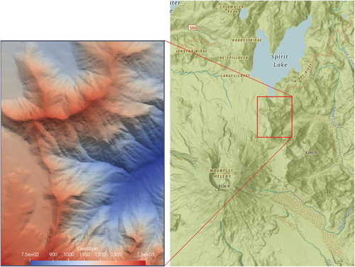
For surface distribution studies, the sources are the sampling points, where the observations and distance scalars are usually treated separately. Therefore, only the topographic data were used for the experiment in this study and random points were used for the sources instead of specific feature points. The experimental topography was a processed TIN from the 0 m LiDAR digital elevation model near Mount Saint Helens. It contains 8,800 elevation points and 17,222 triangles. Of the 8,800 points, there are 4,943 (56.1%) saddle points. The elevation ranges from 751.5 m to 1488.4 m and is rendered as .
Figure 10. Experimental topographic TIN grid rendered in elevation (left). it is located in the region of Mount Saint Helens, near Spirit Lake, Washington, US (right).
3.2 Optimized TIN construction
In scale transformations of topography, many applications require the generation of a TIN with optimized grid-quality. In planar space, the optimized triangulation is often constructed through the Delaunay operation. For each seed in the source points, the 2D Delaunay finds the minimal circumcircles to determine the nearest four neighbors and then constructs the triangulation. It thus provides the maximized minimal angles/minimized maximal circumradii optimization (Cheng, Dey, and Shewchuk Citation2012).
In practice, 2D Delaunay triangulation (D2D) is often used for optimized TIN construction. D2D projects points with elevation onto the level plane (or a designated plane) and then optimizes the triangulation using the 2D Euclidean criterion for judging the minimal circumcircle. The raised TIN grid afterward will inevitably contain non-optimal triangulations that disobey the maximized minimal angle principle.
For each seed on the topographic surface, the GVD cells corresponded to the minimal circumcircles along the surface. Analogous to the definition of planar Delaunay, the dual triangulation of the GVD is then the optimized triangulation. GVD thus contributes to the computationally difficult problem of finding the nearest k neighbors on the non-Euclidean space, which requires super-linear time (Shakhnarovich, Darrell, and Indyk Citation2008) and can be used to justify the potential wrong triangulations from D2D.
On the experimental TIN, 30, 50, 80, and 100 random points were generated as sources and the corresponding GVDs were extracted. The dual TIN was constructed by finding the direct neighbors in the GVD cells. shows the GVD with 30 random sources and the local view of the GVD with the underlying TIN grid. To compare the differences between the GVD dual TIN and the D2D TIN, we overlaid them for examination. shows the GVD dual TIN (green grid) for 30 random sources, and shows the D2D TIN (blue grid) for the same 30 random sources with the GVD dual TIN overlapped; the green edges not covered by the blue ones show the inconsistencies between the two TINs. shows the overlay comparison results for 50 random sources, and shows the results for 100 random sources but with relative uniform distribution. Several inconsistencies are seen between the two kinds of TINs under every sampling resolution.
Figure 11. GVD (green curves) with 30 random sources (yellow points), with a close view on the right.
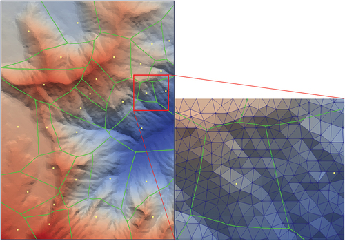
Figure 12. GVD dual TINs compared with the D2D TINs. (a) GVD dual TIN (green) with 30 random sources. (b) D2D TIN (blue) overlaid with the GVD TIN to expose the inconsistent green edges where D2D is potentially incorrect. overlaid TINs for (c) 50 and (d) 100 random sources, with the green edges showing the inconsistencies. The base map consists of the GVD cells rendered with distinct colors.
For the inconsistent triangulations in the different resolutions in , we examined the minimum angles of the triangles indicated by the green edges. The angles of resolution 30 with 7 inconsistencies in are listed in . It can be seen that there are five wrong triangulations from the D2D that did not comply with the maximized minimal angle principle.
Table 1. Maximized minimal angles (°) in the inconsistent triangles between the GVD TIN and the D2D TIN.
Furthermore, pertaining to the inconsistencies in , we examined the areas and area shrunk rate with reference to the original TIN as ground truth. Areas in inconsistent triangulations usually involve quadrilaterals determined in the GVD dual operations. The ground truth area is computed by vertical clipping the original TIN grid with these quadrilaterals. The local area shrunk rate is defined as the percentage of shrunk_area /ground_truth_area. The results are listed in . From , it can be concluded that GVD dual TIN is more conservative in shrinking the topographic surface area than the D2D TIN, since the convex quadrilateral is judged by geodesic rather than the Euclidean metric (which will underestimate the area). The lower area shrunk rate means that the GVD dual transformed surface is closer to the original surface. From an elevation accuracy point of view, the dual triangulation of GVD is more fidelity than the traditional 2D Delaunay triangulation.
Table 2. Areas (m2) and shrunk rate (%) of the inconsistencies in the GVD dual TIN and D2D TIN, referenced to the ground truth areas.
also shows two cases where the D2D TIN was correct while the GVD TIN was incorrect (the blue columns). This is because the edges of the GVD dual structure are polylines of geodesics and are therefore always longer than the straight-line edges of the TIN, which may lead to errors in the maximized minimum angle criterion. In fact, some studies have suggested using the polylines of geodesics instead of straight-line edges as the GVD dual structure for practical use (Liu et al. Citation2017).
Generating a Delaunay TIN with an optimized grid quality is a frequently required routine in geo-computing but is still difficult and locally optimal (Chen and Zhou Citation2013; Dyn, Levin, and Rippa Citation1990). The popularly used D2D method works with a Euclidean criterion, GVD cells can justify the potential errors by checking out the correct minimal circumcircles.
A tightly related choice for an optimized TIN grid is the intrinsic Delaunay triangulation by edge-flipping (Rivin Citation1994), which several contributors have implemented (e.g. Jacobson and Panozzo (Citation2018); Sharp, Soliman, and Crane (Citation2019)). However, the intrinsic Delaunay triangulation works on existing triangular meshes, whereas GVDs seek an optimized triangulation by finding the minimum circumcircles for scale transformation.
3.3 Surface process modeling
An abundance of surface distributions in nature exhibits optimal Voronoi-like patterns, which even appears in the entorhinal cortex of human brains (Hafting et al. Citation2005). In numerical simulation of the surface processes, Voronoi cells often act as the space discretization and serve as the medium of integral for model material, energy, and momentum (Okabe et al. Citation2000).
Before GVD, grid-GVD or raster-GVD (rGVD hereafter) are popular choices for easy implementation (Hu, Liu, and Hu Citation2014; Stewart and Ree Citation2010). rGVD runs very efficiently through facet clustering and differs from the exact GVD only in the boundary facets. Another popular choice is PDE-based GVDs, where skills in interpolation (Peyré and Cohen Citation2006) and linear approximation (Herholz, Haase, and Alexa Citation2017) are generally required. Linear approximation of PDE-based GVDs (lGVD hereafter) produce very well-approximation by taking step-wise subdivision on-demand of the boundary facets. We choose these two kinds of well-approximated GVDs for comparison with the exact GVD.
For a fair comparison, both the rGVD and the lGVD were built on the same exact geodesics of the MMP/VTP algorithm. The refinements of lGVD are as follows (Herholz, Haase, and Alexa Citation2017): locating a singularity on an edge with distinct sources; using singularities per edge to (Delaunay) triangulate the boundary facet; recursively subdivide the boundary facet until no edges contain 2 or more singularities; connecting the singularities with line segments to subdivide the final facets. Since the bisectors are quite straight, as mentioned in Section 2.3, linear subdivision produces very good approximation in practice.
Subdivide along singularities seemed to be the most efficient. However, it often introduced sliver triangles and numerical degenerations (Liu, Zhou, and Hu Citation2007). We implemented the subdivision along the middle point between two adjacent singularities, which works robustly as shown in .
Figure 13. Step-wise subdivision of the boundary facets of TIN mesh in . GVD edge arcs are drawn in green for reference. In (a)/(b), the facet highlighted in purple contains 4 singularities and need to be subdivided. (c) shows the final subdivision with no facet containing 4 or more sources.
The centroidal Voronoi diagram was selected as the surface process model. CVT repeatedly moves the Voronoi centers to the centroids according to some abstract attributes. It is conjectured that, at the iteration convergence, a quasi-uniform hexagonal grid adaptive to distribution of the attribute can be obtained (Du, Faber, and Gunzburger Citation1999; Gersho Citation1979). This adaptive and high-quality grid has a wide range of needs in extensive applications (Du, Gunzburger, and Lili Citation2010; Ye et al. Citation2019). The formula of the CVT iteration is generally written as
where ) is the new center of the Voronoi cell,
is some abstract scalar from observations (e.g. the gray value or the magnitude of the curvature), and Mx and My are the first-order moments of the tessellated cell. A closely related concept developed is the diffusion diagrams or diffusion centroids (Herholz, Haase, and Alexa Citation2017), that is, surface optimization under the free flow of some abstract energy minimization.
Spatial optimization of the CVT relies heavily on repetitions of the Voronoi tessellation. It is therefore a special and ideal checking model for the geometric exactness of the Voronoi cells.
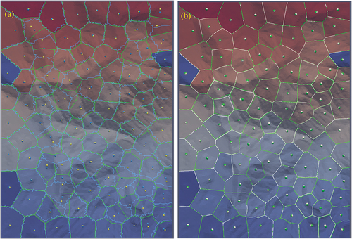
On the experimental TIN, 100 random sources served as sources to generate the GVD, rGVD, and lGVD. shows the initial states and the final states of the sources and GVD cells, respectively. For a clear comparison for the convergence difference, shows an overlay of the final states, indicating that neither rGVD nor lGVD reach the convergence of the exact GVD, while lGVD performs better than rGVD.
Figure 14. Initial states and final states of the exact GVD (a/d), rGvd(b/e), and lGVD (c/f) on CVT optimizations. The same 100 random points are used as the sources. The exact GVD sources and cells are in yellow and green, the rGVD sources and cells are in blue, and the lGVD sources and cells are in white.
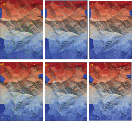
Figure 15. Overlaid final states of the exact GVD and rGVD (a), exact GVD and lGVD (b). The sources and cells of the exact GVD are in yellow and green, the sources and cells of rGVD are in blue, and the sources and cells of lGVD are in white.
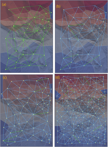
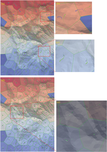
explores the model differences by recording the “diffusion centroid” trajectories during optimization. It can be seen that most centroids of the three VDs evolve in the same optimization directions and come to the denser distribution showing the optimization stop (); however, some centroids of the rGVD move in opposite optimization directions (), some centroids of the lGVD move in biased optimization directions (), while there are still many centroids of the rGVD and lGVD come to early optimization convergence (). Opposite or biased optimization direction means model failure of distorted spatial pattern, while early optimization stop hints low model iteration efficiency.
Figure 16. Trajectories of the GVD (green) diffusion centroids compared with those of rGVD (blue) and lGVD (white). The trajectories of the centroids are sparse at the initial stage and dense at the final stage. (a) comparison of GVD and rGVD. (b) Oppposite optimization directions of rGVD and GVD. (c) early convergence of rGVD than of GVD. (d) comparison of GVD and lGVD. (e) Biased and early stopped optimization of lGVD.
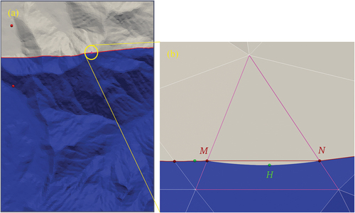
For the rGVD, the stagnation effects from serrated boundaries may explain the convergence failure and efficiency. For the lGVD, difference to the exact GVDs seems quite subtle where most centroids trajectories are in near coincidence. It is known from the analysis in section 2.3 that GVDs need to preserve break points for the shape exactness. For lGVD, it is convenient to locate the break points on boundary facet edges through subdivision, but it is inconvenient to locate the break points inside a facet. Hence, at the facet level, lGVD can produce considerable geometric errors. The though subtle errors accumulated in the CVT optimization and induced biased point pattern. shows another example of bisector on the experimental TIN mesh where the difference between lGVD and exact GVD is hardly discernible at the macro scale but prominent at the facet scale. The break points on edge and inside the boundary facet are drawn to show the shape exactness concept.
Figure 17. Bisector exactness at macro scale and facet scale. (a) hardly discernible difference between the lGVD bisector (red curve) and the exact GVD boundary, with a facet circled in bright yellow for checking. (b) prominent difference found at the facet scale, where a linear scheme directly connected break points on the edge (M/N) for approximation and missed the characteristic edge shape for ignoring the break point (H) inside the facet.
4 Conclusion
Computing the GVD on a topographic surface is as challenging as geodesic distance mapping. This article proposed a new GVD algorithm that resolves the highly complicated and demanding procedure by breaking it up into regular routines. All the operations, such as clustering, structure post-extraction, and conic arrangement-based window growth, are built on consolidated concepts, which effectively solves the algorithm challenges.
The new algorithm is proposed on exact computational geometry approaches because exact computation is more appropriate to the irregular roughness of the Earth’s surface. The key feature of computational geometry approaches is their implicit facet splitting, which gives the GVD construction detailed information and, in the meantime, draws back the efficiency. To avoid overloaded facet splitting, this article presented a gradual window growth method.
The new GVD algorithm is generally suitable in time insensitive scenarios and provides comparable efficiency to the graph approaches and consumes less memory. However, when the accuracy is not so critical (as the CVT checking) or interactive efficiency is required, pre-computation-based graph skills, PDE-based linear approximations are better choices for easy-implementation or super-fast efficiency reasons.
Various crucial applications have been found for GVDs aside from Delaunay triangulation and surface process modeling, such as the minimum spanning tree, point pattern analysis, surface reconstruction, surface interpolation, and geodesic distance descriptor. These must be investigated in future works.
Acknowledgement
We thank the Editor and the anonymous reviewers for their valuable comments which help greatly to improve the article. This work was supported by a grant from State Key Laboratory of Resources and Environmental Information System and the National Natural Science Foundation (No.42230110).
Disclosure statement
The authors declare that they have no known competing financial interests or personal relationships that could have appeared to influence the work reported in this paper.
Data availability statement
The data that support the findings of this study are available in GitHub at: https://github.com/sanchopanza72/gvd_topographic
Notes
References
- Adikusuma, Y. Y., Z. Fang, and Y. He. 2020. “Fast Construction of Discrete Geodesic Graphs.” ACM Transactions on Graphics 39 (2): 1–19. Article 14. doi:10.1145/3144567.
- Aronov, B., M. Berg, and S. Thite 2008. The Complexity of Bisectors and Voronoi Diagrams on Realistic Terrains. The 16th Annual European Symposium, Karlsruhe, Germany, September 15-17, 2008. doi:10.1007/978-3-540-87744-8_9.
- Bobenko, A. I., and B. A. Springborn. 2007. “A Discrete Laplace–Beltrami Operator for Simplicial Surfaces.” Discrete & Computational Geometry 38 (4): 740–756. doi:10.1007/s00454-007-9006-1.
- Bose, P., A. Maheshwari, C. Shu, and S. Wuhrer. 2011. “A Survey of Geodesic Paths on 3D Surfaces.” Computational Geometry 44 (9): 486–498. doi:https://doi.org/10.1016/j.comgeo.2011.05.006.
- Chen, J. 1999. “A Raster-Based Method for Computing Voronoi Diagrams of Spatial Objects Using Dynamic Distance Transformation.” International Journal of Geographical Information Science 13 (3): 209–225. doi:10.1080/136588199241328.
- Cheng, S. -W., T. K. Dey, and J. Shewchuk. 2012. Delaunay Mesh Generation. New York: Chapman & Hall/CRC.
- Chen, J., and Y. Han 1990. Shortest Paths on a Polyhedron. Proceedings of the sixth annual symposium on Computational geometry. Association for Computing Machinery, Berkley, California, USA, 360–369.
- Chen, Y., and Q. Zhou. 2013. “A Scale-Adaptive DEM for Multi-Scale Terrain Analysis.” International Journal of Geographical Information Science 27 (7): 1329–1348. doi:10.1080/13658816.2012.739690.
- Crane, K., M. Livesu, E. Puppo, and Y. Qin 2020. A Survey of Algorithms for Geodesic Paths and Distances. https://ui.adsabs.harvard.edu/abs/2020arXiv200710430C.
- Crane, K., C. Weischedel, and M. Wardetzky. 2013. “Geodesics in Heat: A New Approach to Computing Distance Based on Heat Flow.” ACM Transactions on Graphics 32 (5): 152. doi:10.1145/2516971.2516977.
- Du, Q., V. Faber, and M. Gunzburger. 1999. “Centroidal Voronoi Tessellations: Applications and Algorithms.” SIAM review 41 (4): 637–676. doi:10.1137/S0036144599352836.
- Du, Q., M. Gunzburger, and Lili Ju. 2010. “Advances in Studies and Applications of Centroidal Voronoi Tessellations.” Numerical Mathematics: Theory, Methods and Applications 3 (2): 119–142. doi:10.4208/nmtma.2010.32s.1.
- Dyn, N., D. Levin, and S. Rippa. 1990. “Data Dependent Triangulations for Piecewise Linear Interpolation.” Ima Journal of Numerical Analysis 10 (1): 137–154. doi:10.1093/imanum/10.1.137.
- Elvidge, A. D., I. Sandu, N. Wedi, S. B. Vosper, A. Zadra, S. Boussetta, F. Bouyssel, A. van Niekerk, M. A. Tolstykh, and M. Ujiie. 2019. “Uncertainty in the Representation of Orography in Weather and Climate Models and Implications for Parameterized Drag.” Journal of Advances in Modeling Earth Systems 11 (8): 2567–2585. doi:10.1029/2019ms001661.
- Gersho, A. 1979. “Asymptotically Optimal Block Quantization.” IEEE Transactions on Information Theory 25 (4): 373–380. doi:10.1109/TIT.1979.1056067.
- Hafting, T., M. Fyhn, S. Molden, M. B. Moser, and E. I. Moser. 2005. “Microstructure of a Spatial Map in the Entorhinal Cortex.” Nature 436 (7052): 801–806. doi:10.1038/nature03721.
- Herholz, P., and M. Alexa. 2018. “Factor Once: Reusing Cholesky Factorizations on Sub-Meshes.” ACM Transactions on Graphics 37 (6): 1–9. Article 230. doi:10.1145/3272127.3275107.
- Herholz, P., F. Haase, and M. Alexa. 2017. “Diffusion Diagrams: Voronoi Cells and Centroids from Diffusion.” Computer Graphics Forum 36 (2): 163–175. doi:https://doi.org/10.1111/cgf.13116.
- Hu, H., X. Liu, and P. Hu. 2014. “Voronoi Diagram Generation on the Ellipsoidal Earth.” Computers & Geosciences 73: 81–87. doi:10.1016/j.cageo.2014.08.011.
- Jacobson, A., and D. Panozzo 2018. Libigl: A Simple C++ Geometry Processing Library.
- Kanai, T., and H. Suzuki. 2001. “Approximate Shortest Path on a Polyhedral Surface and Its Applications.” Computer-Aided Design 33 (11): 801–811. doi:10.1016/S0010-4485(01)00097-5.
- Kimmel, R., and J. A. Sethian. 1998. “Computing Geodesic Paths on Manifolds.” Proceedings of the National Academy of Sciences 95 (15): 8431–8435. doi:10.1073/pnas.95.15.8431.
- Lanthier, M. A. 1999. Shortest path problems on polyhedral surfaces. Ph.D, Carleton University
- Liu, C. H. 2018. “A Nearly Optimal Algorithm for the Geodesic Voronoi Diagram of Points in a Simple Polygon.” Algorithmica 82 (4): 915–937. doi:10.1007/s00453-019-00624-2.
- Liu, Y. -J., Z. Chen, and K. Tang 2011. Construction of Iso-Contours, Bisectors, and Voronoi Diagrams on Triangulated Surfaces. IEEE Transactions on Pattern Analysis and Machine Intelligence, 33, 1502–1517, doi: 10.1109/TPAMI.2010.221.
- Liu, Y. J., D. Fan, C. X. Xu, and Y. He. 2017. “Constructing Intrinsic Delaunay Triangulations from the Dual of Geodesic Voronoi Diagrams.” ACM Transactions on Graphics 36 (2): 43–57. doi:10.1145/2999532.
- Liu, Y., M. F. Goodchild, Q. Guo, Y. Tian, and L. Wu. 2008. “Towards a General Field Model and Its Order in GIS.” International Journal of Geographical Information Science 22 (6): 623–643. doi:10.1080/13658810701587727.
- Liu, Y. -J., Q. -Y. Zhou, and S. -M. Hu. 2007. “Handling Degenerate Cases in Exact Geodesic Computation on Triangle Meshes.” The Visual Computer 23 (9–11): 661–668. doi:10.1007/s00371-007-0136-5.
- Mitchell, J. S. B., D. M. Mount, and C. H. Papadimitriou. 1987. “The Discrete Geodesic Problem.” Siam Journal on Computing 16 (4): 647–668. doi:10.1137/0216045.
- Nazzaro, G., E. Puppo, and F. Pellacini. 2021. “geoTangle: Interactive Design of Geodesic Tangle Patterns on Surfaces.” ACM Transactions on Graphics 41 (2): 1–17. Article 12. doi:10.1145/3487909.
- Okabe, A., B. Boots, K. Sugihara, and S. N. Chiu. 2000. Spatial Tessellations: Concepts and Applications of Voronoi Diagrams. 2 ed. Chichester: JOHN WILEY & SONS.
- Papadopoulou, E., and D. T. Lee. 1998. “A New Approach for the Geodesic Voronoi Diagram of Points in a Simple Polygon and Other Restricted Polygonal Domains.” Algorithmica 20 (4): 319–352. doi:10.1007/PL00009199.
- Peyré, G., and L. D. Cohen. 2006. “Geodesic Remeshing Using Front Propagation.” International Journal of Computer Vision 69 (1): 145–156. doi:10.1007/s11263-006-6859-3.
- Qin, Y., X. Han, H. Yu, Y. Yu, and J. Zhang. 2016. “Fast and Exact Discrete Geodesic Computation Based on Triangle-Oriented Wavefront Propagation.” ACM Transactions on Graphics 35 (4): 125. doi:10.1145/2897824.2925930.
- Qin, Y., H. Yu, and J. Zhang. 2017. “Fast and Memory-Efficient Voronoi Diagram Construction on Triangle Meshes.” Computer Graphics Forum 36 (5): 93–104. doi:https://doi.org/10.1111/cgf.13248.
- Rivin, S. 1994. “Euclidean Structures on Simplicial Surfaces and Hyperbolic Volume.” Annals of Mathematics 139 (3): 553–580. doi:10.2307/2118572.
- Shakhnarovich, G., T. Darrell, and P. Indyk. 2008. “Nearest-Neighbor Methods in Learning and Vision.” IEEE Transactions on Neural Networks 19 (2): 377–377. doi:10.1109/TNN.2008.917504
- Sharir, M., and A. Schorr. 1986. “On Shortest Paths in Polyhedral Spaces.” Siam Journal on Computing 15 (1): 193–215. doi:10.1137/0215014.
- Sharp, N., Y. Soliman, and K. Crane. 2019. “The Vector Heat Method.” ACM transactions on graphics 38 (3): 24.21–24.19. doi:10.1145/3243651
- Smith, M. W. 2014. “Roughness in the Earth Sciences.” Earth-Science Reviews 136: 202–225. doi:10.1016/j.earscirev.2014.05.016.
- Stewart, C. W., and R. Ree. 2010. “A Voronoi Diagram Based Population Model for Social Species of Wildlife.” Ecological modelling 221 (12): 1554–1568. doi:10.1016/j.ecolmodel.2010.03.019.
- Surazhsky, V., T. Surazhsky, D. Kirsanov, S. Gortler, and H. Hoppe. 2005. “Fast Exact and Approximate Geodesics on Meshes.” ACM Transactions on Graphics 24 (3): 553–560. doi:10.1145/1073204.1073228.
- Wang, X., Z. Fang, J. Wu, S. Q. Xin, and Y. He. 2017. “Discrete Geodesic Graph (DGG) for Computing Geodesic Distances on Polyhedral Surfaces.” Computer Aided Geometric Design 52: 262–284. doi:10.1016/j.cagd.2017.03.010.
- Xiang, Y., S. Q. Xin, and H. Ying. 2014. “Parallel Chen-Han (PCH) Algorithm for Discrete Geodesics.” ACM Transactions on Graphics 33: 1–11. doi:10.1145/2534161.
- Xin, S. Q., and G. J. Wang. 2009. “Improving Chen and Han’s Algorithm on the Discrete Geodesic Problem.” ACM Transactions on Graphics 28 (4): 1–8. doi:10.1145/1559755.1559761.
- Xin, S., W. Wang, Y. He, Y. Zhou, S. Chen, C. Tu, and Z. Shu. 2018. “Lightweight Preprocessing and Fast Query of Geodesic Distance via Proximity Graph.” Computer-Aided Design 102: 128–138. doi:10.1016/j.cad.2018.04.021.
- Xu, C., Y. Liu, S. Qian, J. Li, and H. Ying. 2015. “Polyline-Sourced Geodesic Voronoi Diagrams on Triangle Meshes.” Computer Graphics Forum 33 (7): 161–170. doi:10.1111/cgf.12484.
- Xu, C., T. Y. Wang, Y. J. Liu, L. Liu, and Y. He. 2015. “Fast Wavefront Propagation (FWP) for Computing Exact Geodesic Distances on Meshes.” IEEE Transactions on Visualization & Computer Graphics 21 (7): 822. doi:10.1109/TVCG.2015.2407404.
- Ye, Z., R. Yi, M. Yu, Y. J. Liu, and Y. He. 2019. “Geodesic Centroidal Voronoi Tessellations: Theories.” Algorithms and Applications. doi:10.48550/arXiv.1907.00523.
- Ying, X., X. Wang, and Y. He. 2013. “Saddle Vertex Graph (SVG): A Novel Solution to the Discrete Geodesic Problem.” ACM Transactions on Graphics 32 (6): 1–12. doi:10.1145/2508363.2508379.
- Zayer, R., D. Mlakar, M. Steinberger, and H. -P. Seidel. 2018. “Layered Fields for Natural Tessellations on Surfaces.” ACM Transactions on Graphics 37 (6): 1–15. Article 264. doi:10.1145/3272127.3275072.