Tree species classification in a typical natural secondary forest using UAV-borne LiDAR and hyperspectral data

ABSTRACT

Recent growth in unmanned aerial vehicle (UAV) technology have promoted the detailed mapping of individual tree species. However, the in-depth mining and comprehending of the significance of features derived from high-resolution UAV data for tree species discrimination remains a difficult task. In this study, a state-of-the-art approach combining UAV-borne light detection and ranging (LiDAR) and hyperspectral was used to classify 11 common tree species in a typical natural secondary forest in Northeast China. First, comprehensive relevant structural and spectral features were extracted. Then, the most valuable feature sets were selected by using a hybrid approach combining correlation-based feature selection with the optimized recursive feature elimination algorithm. The random forest algorithm was used to assess feature importance and perform the classification. Finally, the robustness of features derived from point clouds with different structures and hyperspectral images with different spatial resolutions was tested. Our results showed that the best classification accuracy was obtained by combining LiDAR and hyperspectral data (75.7%) compared to that based on LiDAR (60.0%) and hyperspectral (64.8%) data alone. The mean intensity of single returns and the visible atmospherically resistant index for red-edge band were the most influential LiDAR and hyperspectral derived features, respectively. The selected features were robust in point clouds with a density not lower than 5% (~5 pts/m²) and a resolution not lower than 0.3 m in hyperspectral data. Although canopy surface features were slightly different from original LiDAR features, canopy surface information was also important for tree species classification. This study proved the capabilities of UAV-borne LiDAR and hyperspectral data in natural secondary forest tree species discrimination and the potential for this approach to be transferable to other study areas.

KEYWORDS:

• Unmanned aerial vehicle (UAV)
• light detection and ranging (LiDAR)
• hyperspectral imaging
• tree species classification
• feature selection

1. Introduction

Tree species information is fundamental to our understanding of terrestrial ecosystems (Cazzolla Gatti et al. 2022). Detailed tree species composition and spatial distribution are essential for many applications, including forest resource dynamic monitoring (van Aardt and Wynne 2007), sustainable forest management (Dalponte, Bruzzone, and Gianelle 2012), ecosystem service quantification (Boerema et al. 2017), biodiversity assessment (Piiroinen et al. 2018). Tree species can also be used as an input for species-specific tree allometry models (Ørka et al. 2013), which is important for calculating vegetation growing stock volume, biomass or carbon storage estimation (Kirby and Potvin 2007; Korpela and Erkki Tokola 2006). Remote sensing-assisted tree species discrimination has been in development for nearly four decades (Fassnacht et al. 2016). It is cost-efficient and can be used to rapidly map the distribution of tree species over different space scales compared to traditional field tree species surveys (Masek et al. 2015). However, most remote sensors are carried on satellites or manned aircraft, and it is difficult to balance both spectral and spatial resolution (Goodbody et al. 2017).

In recent years, a flexible, convenient and affordable unmanned aerial vehicle (UAV) platform has gradually emerged, and it has shown the great capability for obtaining small-scale forest inventories (Colomina and Molina 2014; Hao et al. 2022). By collecting very high spatial or spectral resolution data, UAVs can increase opportunities for tree species classification (Zhang, Zhao, and Zhang 2020). Many small-sized and lightweight sensors carried on UAVs, such as RGB cameras, multispectral/hyperspectral imagers and laser scanners have been used for tree species discrimination (Schiefer et al. 2020; Zhong et al. 2020). Each of these sensors has its strengths, for example, hyperspectral data usually ranges hundreds of narrow continuous bands and can acquire more refined spectral responses (Schaepman-Strub et al. 2006). Some advanced UAV-borne hyperspectral data that can take into account both spectral and spatial resolution have emerged in the discrimination of tree species (Adão et al. 2017). Light detection and ranging (LiDAR) data can describe the three-dimensional architecture of the forest canopy, with important implications for tree species mapping (Coops et al. 2007). Research in the past decade has shown the advantage of combining hyperspectral and LiDAR datasets is that the spectral reflectance characteristics and spatial structure characteristics of tree species can be well represented (Dian et al. 2016; Zhongya et al. 2016). The state-of-art technology is to integrate UAV-borne hyperspectral imaging (UHSI) and laser scanning (ULS) data to achieve a double boost in spatial and spectral resolution so that more detailed background signals and characterization of canopies can be obtained in individual tree-based classification (Schiefer et al. 2020).

Revolutionary breakthroughs in data resolution for near-ground UAV systems are a double-edged sword. On the one hand, these very high-resolution measurements can capture rich information about tree canopies. For example, different wavelengths of hyperspectral data can reflect vegetation: 1) photosynthetic pigment content (e.g. chlorophyll, carotenoids and anthocyanins) (Clark and Roberts 2012), 2) water content (Asner 1998), and 3) leaf structure/morphology (e.g. leaf area index, thickness of cell walls) (Fricker et al. 2015). High spatial resolution imagery can reflect crown texture information, such as the roughness of the crown surface, the size and arrangement of branches and leaves, the shadows inside the crown (Fassnacht et al. 2016). High-density ULS data can nearly completely reconstruct the 3D structure of trees, and further reflecting the morphology of branches and the distribution of foliage within a crown (Yifang et al. 2018; Michałowska and Rapiński 2021). The intensity information is also related to leaf type, area, orientation, clustering and gap (Korpela et al. 2010). But on the other hand, feature mining is by no means easy. Although numerous hyperspectral and LiDAR-derived variables have been proposed to describe these characteristics relevant to tree species classification (Ruiliang 2021), previous studies often considered only a few of these variables and lacked a comprehensive understanding of the characteristics of the data.

Moreover, such massive features brought by high-resolution UAV data usually cause redundancy and multicollinearity, which can complicate classification (Yifang et al. 2018). For feature dimensionality reduction, many studies directly used the variable importance rankings in the decision tree model (Wai Tim et al. 2017; Zhong et al. 2020). However, this ranking does not take into account the collinearity between variables, resulting in pseudo variable importance (Wang et al. 2022). Some studies used correlation-based methods (Liu et al. 2017) or stepwise variable selection (Wang et al. 2022) or combined these two methods (Zhou et al. 2022) to address this issue. But a more efficient variable selection procedure deserves further consideration to increase our understanding of what specifically drives tree species discrimination. In addition, these UAV-derived features are affected by many factors, such as sensor performance, system errors and flight parameters (Rana et al. 2022), which are difficult to directly transplant to other research fields, which greatly limits the application of UAVs.

Natural secondary forests occupy approximately 46.2% of China’s forests (Zhang, Dong, and Liu 2020). It is characterized by high tree species diversity, high canopy closure, and is dominated by broad-leaved trees. Therefore, tree species classification in natural secondary forests is still a great challenge. Recent studies have conducted explorations of the combination of ULS and UHSI for tree species discrimination in different forest conditions, such as urban forest parks (Hartling, Sagan, and Maimaitijiang 2021), subtropical broadleaf forests (Qin et al. 2022) and mangrove forests (Cao et al. 2021). However, tree species classification in natural secondary forests has rarely been explored.

Therefore, given the above-mentioned problems, this study explored the utilization of a hybrid feature selection procedure for tree species classification in typical natural secondary forests by combining ULS and UHSI data. The specific goals of the study were as follows: (1) to generate detailed geometric and radiometric variables from ULS data and spectral and texture variables from UHSI, (2) to select the most valuable ULS and UHSI feature sets and combine these features for tree species discrimination, and (3) to assess and analyze the robustness of these selected features under a simulation application.

2. Materials and methods

2.1. Study region and field measurements

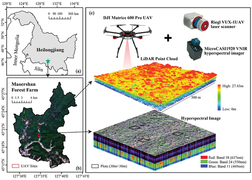
The typical natural secondary forest situated in Maoershan Forest Farm, Shangzhi, Heilongjiang Province, Northeast China (127°29′–127°44′ E, 45°14′–45°29′ N) was selected as the study region (Figure 1). It is dominated by broad-leaved forest and accompanied by a small number of coniferous plantations, such as Korean pine and larch. In this study, a total of 7 sites were established with an area of 9 hectares, and each site was evenly distributed with 3 sample square plots with a width of 30 m.

Figure 1. (A) the location of Maoershan forest farm; (b) the Sentinel-2 image of Maoershan acquired on 21 May 2016 and the location of UAV sites; (c) LiDAR and hyperspectral data from a UAV site and photos of UAV and sensors. The projection coordinate system used for all data in this study is WGS 1984 UTM Zone 52 N.

Field data were collected during August 2021 (leaf-on season). It mainly included tree species and location information of trees with diameter at breast height (DBH) greater than 5 cm. This study used a Qianxun SR3 Pro network real-time kinematic (RTK) to measure the tree trunk positions and four corner positions of each plot with centimeter-level accuracy. The coordinates of trees relative to the plot boundaries were also recorded by a hand-held laser rangefinder, which were used as supplementary information for poor GNSS single tree positioning. The root mean square errors between the RTK-positioned sample trees and their georeferenced relative coordinates were about 0.3–0.5 m. In total, 11 main tree species were recorded, which can be divided into two types: 1) broadleaf species, including Mono maple (Acer mono), White birch (Betula platyphylla), Walnut (Juglans mandshurica), Manchurian ash (Fraxinus mandshurica), Cork tree (Phellodendron amurense), Dahurian poplar (Populus davidiana), Mongolian oak (Quercus mongolica), Basswood (Tilia), elm (Ulmus); and 2) conifer species, including larch (Larix olgensis) and Korean pine (Pinus koraiensis).

2.2. UAV-borne data collection and preprocessing

2.2.1. ULS data

ULS data for all sites were collected from September 4–6, 2021, using a Riegl VUX-1UAV laser scanner mounted on the DJI Matrice 600 Pro UAV. The flight altitude of the ULS system was between 120–370 meters above ground level due to the undulating terrain in the survey area, and the speed was 10 m/s. All flights were designed as crossing routes with 60 m spacing to guarantee point cloud quality. The scanning angle was interpreted within ±45°. The average point density was approximately 320–360 pulses/m². For each site, the LiDAR data were preprocessed, and the main steps include point cloud denoising, point cloud filtering, point cloud rasterization, and height normalization. First, ground points were filtered and digital terrain models (DTMs) were generated (Guo et al. 2010). Subsequently, the Z-values of the original point clouds were subtracted from the corresponding DTMs to obtain the height relative to the ground, and canopy surface points (CSPs) were filtered by using a graph-based progressive morphological filtering (GPMF) algorithm (Hao et al. 2019). Finally, pit-free canopy height models (CHMs) with 0.1 m spatial resolution were interpolated by CSPs (Quan et al. 2021). Data preprocessing was performed by LiDAR360 V4.0 software and MATLAB R2021a.

2.2.2. UHSI data

UHSI data were acquired from September 8–10, 2021, on sunny clear-sky days around noon using a portable MicroCASI1920 pushbroom VNIR hyperspectral imager (https://www.itres.com/wp-content/uploads/2019/09/MicroCASI_1920_specsheet.pdf) mounted on the same drone as the laser scanner. The flying speed was 5 m/s, and the altitude was between 250–340 meters above ground level. The scan angle of the imager was 36.6° and the lateral overlap of the flight was set to 40%. Images with 288 spectral channels (400–1000 nm) and 0.1 m spatial resolution were generated. Considering excessive band redundancy, the original bands were resampled to 96 spectral bands (spectral width of 6.3 nm) by the data provider using the Bi-section method in RCX software (ITRES Research Ltd., Canada). Geometric calibration and radiometric correction of the hyperspectral images were also accomplished by RCX software. Atmospheric correction was done by ENVI 5.3 software FLAASH module. Finally, all hyperspectral images and CHMs were co-registered using control points collected manually from CHMs (the error was less than one pixel), and all preprocessed data were clipped with 5 m buffer plot boundaries for subsequent applications. The whole research workflow was shown in Figure 2.

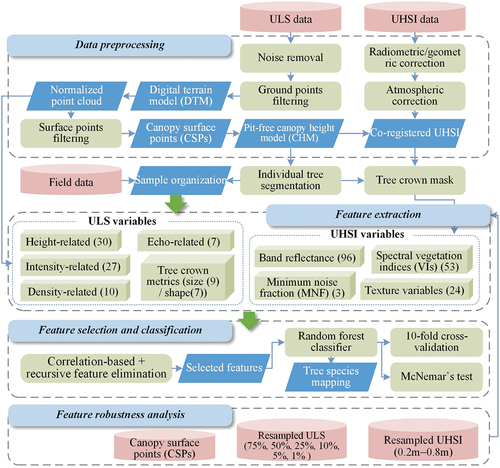
Figure 2. Research workflow of this study.

2.3. Individual tree segmentation and sample organization

For visual detectability in both LiDAR and hyperspectral data, we chose a CHM-based individual tree segmentation method to automatically detect and delineate trees, which is named region-based hierarchical cross-section analysis (RHCSA). This approach is a top-down detection method, by detecting the relationship among the tree crowns in the horizontal plane to determine whether to split them (Zhao et al. 2017). The RHCSA was developed based on natural secondary forests, and previous studies have demonstrated its ability to segment individual tree crowns under different forest stand types (Yinghui et al. 2022; Zhen et al. 2022).

After segmenting individual trees, we matched each detected tree with the field samples with the assistance of the collected tree locations and RGB images synthesized from the hyperspectral image. Trees undetected and matched to more than one detected tree were removed. The laser points of each correct segment were labeled with the corresponding field measurement tree species for the derivation of LiDAR features. To eliminate the influence of shrubs and herbs, tree points with heights <2 m were removed, and we manually pruned the segmented point cloud to ensure the purity of the sample data. As a result, 904 sample trees of the 11 species were retained for further classification (Table 1). The examples are displayed in Figure 3.

Figure 3. Examples of data visualization for 11 tree species, each sample includes its 0.1 m resolution CHM (top left), 0.1 m resolution RGB image synthesized from the hyperspectral image (bottom left) and the point cloud (right).

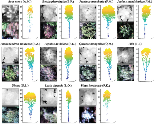
Table 1. Number of samples for 11 species and corresponding abbreviations.

Forest Type	Tree Species	Abbreviations	Samples
Broadleaved	Acer mono	A.M.	86
	Betula platyphylla	B.P.	123
	Fraxinus mandshurica	F.M.	186
	Juglans mandshurica	J.M.	142
	Phellodendron amurense	P.A.	16
	Populus davidiana	P.D.	63
	Quercus mongolica	Q.M.	26
	Tilia	T.I.	71
	Ulmus	U.L.	125
Coniferous	Larix olgensis	L.O.	21
	Pinus koraiensis	P.K.	45

2.4. Feature extraction

2.4.1. ULS feature extraction

ULS features were extracted from all labeled individual tree laser points and classified into five categories: 1) height-related variables, 2) intensity-related variables, 3) density-related variables, 4) echo-related variables, and 5) tree crown metrics. In addition to some basic metrics that can reflect the point distributions and radiometric information, a series of crown metrics describing the crown size and crown shape were calculated from the high-density ULS data. The crown size-related LiDAR metrics included crown length, diameter, volume, surface area, projected area, and perimeter. The crown shape was expressed as the roundness of the crown projection in the horizontal direction, and as the contour shape of the crown outer edges in the vertical direction (Gao, Huiquan, and Fengri 2017). Based on our previous study of crown profile modeling using ULS data (Quan et al. 2020), the basic parabola equation was used to fit the crown profile and the two equation coefficients were estimated to quantify crown shape. Moreover, the ratio of some crown metrics was also calculated to describe the crown shape. A full description of all LiDAR features is shown in Supplementary Material Table S1.

2.4.2. Hyperspectral feature extraction

For hyperspectral features, we first overlaid the vector crown boundaries delineated from the CHMs with the hyperspectral image and then calculated the hyperspectral features of each crown. The mean spectral reflectance of each band (b1–b96) within each tree crown was calculated, and the components 1–3 of the minimum noise fraction (MNF) rotation were also used to band dimensionality (Green et al. 1988). The third category of variable is spectral vegetation indices (VIs), which express the combination of bands through different mathematical formulas (Ali et al. 2017). Herein, a total of 53 VIs were calculated, which were divided into three categories: 1) structural, 2) pigment (such as chlorophyll, anthocyanin/carotenoid), and 3) physiological. Then, 24 texture features were computed from the RGB bands, and each band has 8 features. A full description of these hyperspectral features is shown in Supplementary Material Table S2. To reduce the effect of shadowing and nonvegetation pixels, we masked all pixels with normalized vegetation index (NDVI) < 0.5, near-infrared reflectance (NIR) < 0.2 and CHM <4 m (Piiroinen et al. 2018). Both LiDAR and hyperspectral features were generated using MATLAB R2021a. Standardization of the feature dataset was conducted to convert features to zero mean and unit variance before classification (Rana et al. 2022).

2.5. Feature selection

This study utilized a hybrid approach for selecting features in the classification model. By combining correlation-based feature selection (CFS) with the optimized recursive feature elimination (RFE) algorithm, important and meaningful variables were selected as inputs for the subsequent classification model. RFE is a backwards selection method that continuously finds the optimal subset of features (Gregorutti, Michel, and Saint-Pierre 2017). In this study, the RFE algorithm was optimized by retraining a random forest (RF) model and recomputing feature importance in each iteration (Figure 4).

Figure 4. Flowchart of the feature selection.

According to the flowchart, the feature selection procedure was conducted with the following steps:

1. Train an RF model on the initial set of features and compute the permutation importance (also known as the mean decrease accuracy (MDA));

2. Cluster highly correlated features using Spearman’s correlation coefficient (|r| ≥ 0.9) and retain (Rana et al. 2022) the variable with the highest ranking of importance in each cluster;

3. Retrain an RF using the retained features and compute the permutation importance;

4. Eliminate the least important variables from the current set of features;

5. Repeat steps (3-4) until only one feature remains and output the remaining variables in each recursion and the corresponding overall accuracy (OA);

Ultimately, the minimum number of variables that met the accuracy requirements were chosen for the final classification.

2.6. RF classification and accuracy assessment

RF methodology is a mature and popular machine learning algorithm and is frequently used in tree species classification (Belgiu and Drăgu 2016). The RF is a nonparametric model that ensembles an abundance of single independent decision trees (Breiman 2001). The advantages of the RF method are that it is computationally fast, internally verified to calculate the error matrix, less sensitive to overfitting and is able to derive the importance of variables (Ruiliang 2021). It can also handle unbalanced data with missing values compared to other classifiers (Pal 2005). In this study, the RF model was executed with scikit-learn v0.24.2 (Pedregosa et al. 2011), and a RandomizedSearchCV function (Bergstra, James, and Yoshua 2012) was used to determine the optimal hyperparameter combination for the classifier with stratified fivefold random cross-validation.

The precision (user’s accuracy, UA), recall (producer’s accuracy, PA) and F1-score were used to evaluate the classification results for each tree species. The macro and weighted average of these three metrics, as well as the OA were used to evaluate the overall results (Mäyrä et al. 2021) by performing 10-fold cross-validation. McNemar’s test was also employed to decide if the classification results differed significantly from one another (McNemar 1947). All feature selection and classification were implemented using the Python programming language.

2.7. Feature robustness analysis

We conducted simulation experiments to analyze the robustness of features under different UAV imaging conditions. Given the flexibility and autonomous opportunity of UAVs, the pre-defined flight height and speed directly influence the spatial resolution of the collected data (Ruiliang 2021). Therefore, we randomly sampled ULS returns with different percentages (i.e. 75%, 50%, 25%, 10%, 5%, and 1%) (Hao et al. 2022) and resampled UHSI data at spatial resolutions of 0.2–0.8 m by nearest neighbor assignment method to stimulate the reuse robustness of the selected features for classification in different spatial resolution data. Features were recalculated from the thinned point clouds and resampled images.

In addition to the spatial resolution, the spatial distribution of the point cloud is also affected by ULS sensors. Since not all laser scanners have multiple echoes capabilities and imagery sensors can mainly capture the surface structure of the canopy (such as photogrammetric point clouds), we simulated canopy surface information using the GPMF algorithm. The same LiDAR features were extracted from CSPs generated by GPMF and used for classification to test the robustness of features in point clouds distributed on the canopy surface. A specific introduction to the GPMF can be found in Hao et al. (2019). For the evaluation of features, in addition to the RF importance, we also used a paired T test to determine if the features derived from the simulated data are significantly different from that of the original data.

3. Results

3.1. Feature selection

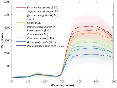
The spectral curve for each of the 11 species ranging 400–1000 nm was shown in Figure 5. All tree species had similar reflectance in the visible spectral range. The F.M. (see Table 1 for acronym meaning) had the highest NIR reflectance, while the P.A. had significantly lower reflectance than other species. The Q.M. and T.I., U.L. and P.D. and L.O. and A.M. were three pairs of classes that exhibited high visual similarity from Figure 5. The results showed that there were similar spectral reflectance values among many tree species, and even conifers and deciduous trees were difficult to distinguish based on spectral values.

Figure 5. The mean and ± 1 standard deviation of the spectral reflectance (×10000) for all 11 tree species.

A high correlation emerged among many of the LiDAR and hyperspectral features. After CFS clustering, 30 out of 90 ULS features and 35 out of 176 UHSI features were retained. The specific recursive elimination processes of the retained features and the corresponding accuracy are shown in Figure 6. When the number of features was decreased using the optimized RFE, the OA changed gradually at first and then rapidly decreased. The final features were selected by weighing the number of features and the OA. Eventually, 9 LiDAR features and 11 hyperspectral features were selected for subsequent classification. These features included 3 height-related variables, 1 intensity-related variable, 1 density-related variable, 2 echo-related variables, 2 tree crown metrics, 2 spectral transformation variables and 9 vegetation indices (Table 2).

Figure 6. The number of features used in RFE versus the overall accuracy based on 10-fold cross-validation.

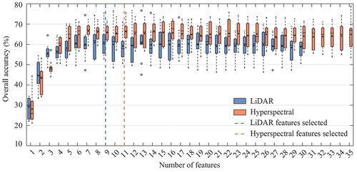
Table 2. List of selected features and descriptions.

Features	Description
LiDAR (9)
H1	1th percentile of heights
H99	99th percentile of heights
Hmad	Median absolute deviation of height
I5	5th percentile of intensity
D10	Proportion of points in the 10th bin (from bottom to top) to total number of points
Imean_single	Mean intensity of single returns
Last_all_ratio	Proportion of last returns above 2 m
RCD	Ratio of crown length to average crown diameter
CD_std	Standard deviation of crown diameter calculated by 2D convex hull of tree points projection in the horizontal direction
Hyperspectral (11)
MNF1	1st component of minimal noise fraction
MNF2	2nd component of minimal noise fraction
BGI	Blue green pigment index
DD	Double difference
GI	Greenness index
NPCI	Normalized pigment chlorophyll ratio index
RVSI	Red-edge vegetation stress index
NPQI	Normalized phaeophytinization index
TCI	Triangle chlorophyll VI
PRI	Photochemical/physiological reflectance index
VARI_red_edge	Visible atmospherically resistant index for red-edge band

3.2. Comparison of classification accuracies

The results of the classification (Table 3) indicated that combining LiDAR and hyperspectral features significantly increased the OA from 60.0% (LiDAR) and 64.8% (hyperspectral) to 75.7% (McNemar’s test, p < 0.05). Using hyperspectral data provided significantly higher accuracy than using LiDAR data (McNemar’s test, p < 0.05). P.K., L.O. and F.M. obtained the highest F1-score (86.7%, 81.8% and 88.2%) when using LiDAR, hyperspectral and combined data, respectively. P.A. has the lowest classification accuracy, regardless of the data used.

Table 3. Classification results using different feature combinations.

	LiDAR			Hyperspectral			LiDAR + Hyperspectral
Tree species	UA(%)	PA(%)	F1%)	UA(%)	PA(%)	F1%)	UA(%)	PA(%)	F1%)
A.M.	37.7	30.2	33.5	54.4	57.0	55.7	60.8	55.8	58.2
B.P.	64.0	72.4	67.9	63.0	70.7	66.7	75.4	87.0	80.8
F.M.	69.5	74.7	72.0	75.4	85.5	80.1	86.2	90.3	88.2
J.M.	70.7	81.7	75.8	75.2	78.9	77.0	85.3	90.1	87.7
P.A.	0.0	0.0	0.0	50.0	25.0	33.3	75.0	37.5	50.0
P.D.	38.1	25.4	30.5	54.2	41.3	46.8	66.7	63.5	65.0
Q.M.	42.1	30.8	35.6	64.7	42.3	51.2	71.4	57.7	63.8
T.I.	49.2	43.7	46.3	54.9	39.4	45.9	60.3	57.7	59.0
U.L.	48.0	58.4	52.7	47.4	50.4	48.8	63.2	63.2	63.2
L.O.	66.7	38.1	48.5	78.3	85.7	81.8	89.5	81.0	85.0
P.K.	94.7	80.0	86.7	80.6	64.4	71.6	94.6	77.8	85.4
OA(%)	60.0			64.8			75.7
Macro avg(%)	52.8	48.7	50.0	63.5	58.2	59.9	75.3	69.2	71.5
Weighted avg(%)	58.3	60.0	58.7	64.3	64.8	64.1	75.5	75.7	75.3

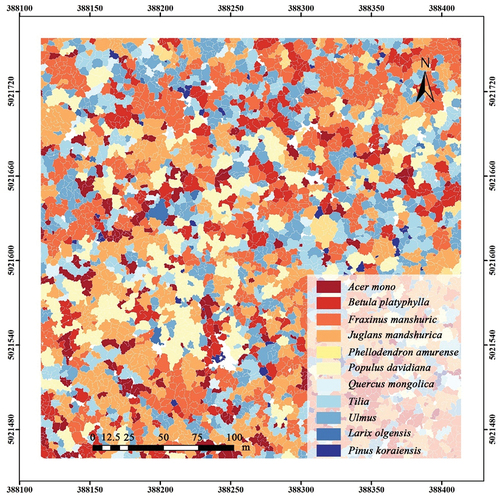
Confusion matrices were used to gain more insight into the details of misclassification, as shown in Figure 7. When using only LiDAR features, some of the P.D. were wrongly classified as B.P. and F.M.; A.M. and T.I. and F.M. and U.L. were also misclassified. Almost half of L.O. were classified as F.M., but when hyperspectral features were used, the situation was completely reversed. When using only hyperspectral features, the P.D. and T.I. were wrongly classified as the U.L. and U.L. were misclassified as B.P. Regardless of the features used, P.A. were always wrongly classified as B.P. Combining LiDAR and hyperspectral features effectively reduced both omission and commission errors for tree species, except for A.M., L.O. and P.K. The optimal classification results were achieved for A.M. and L.O. when only hyperspectral data were used, and the optimal classification results were achieved for P.K. when only LiDAR data were used. The distribution of tree species prediction results using the best feature combination is shown in Figure 8.

Figure 7. Confusion matrices for different input features (rows: field measured species; columns: predicted species).

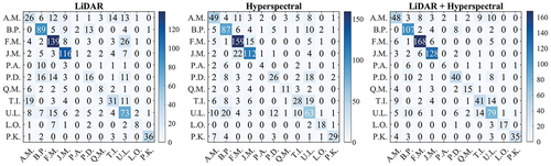
Figure 8. Tree species distribution map using combined ULS and UHSI data for the same UAV site example as in Figure 1.

3.3. Importance of selected features

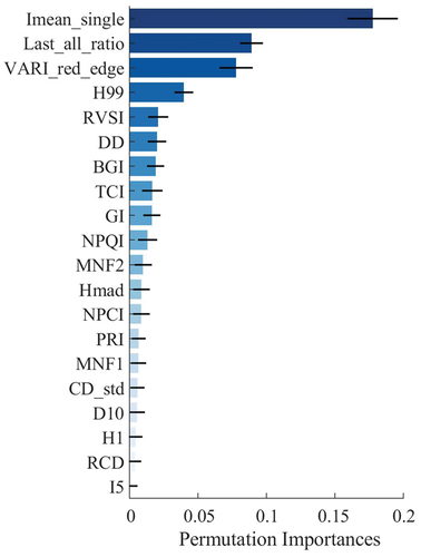
The permutation importance and ranking for classification based on ULS and UHSI data of the 20 selected variables are presented in Figure 9. Imean_single was the most important feature, followed by Last_all_ratio, VARI_red_edge and H99. Seven out of the 10 top-ranked features were VIs. Tree crown metrics (CD_std and RCD) and small percentiles of height and intensity variables (H1 and I5) ranked low overall.

Figure 9. The permutation importance of the final variables for classification.

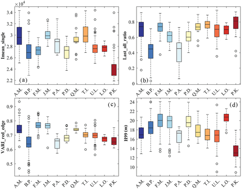
The differences in the 4 top-ranked features among the 11 tree species are plotted in Figure 10. The figure shows that the 4 features varied among the 11 tree species. The values of Imean_single (Figure 10a) and H99 (Figure 10d) for P.K. were clearly lower than that for other species. F. M and J.M. were most easily separated by VARI_red_edge (Figure 10c). Similarly, P.B. and P.A. were most easily separated by Last_all_ratio (Figure 10b). At times, it was difficult to distinguish species based on a single feature; for example, B.P. and F.M. had similar Imean_single values. Multiple features complement each other, facilitating the separation of multiple tree species.

Figure 10. Box plots of the top 4 ranked features: (a) Imean_single; (b) Last_all_ratio; (c) VARI_red_edge and (d) H99 among 11 tree species.

3.4. Robustness analysis of features

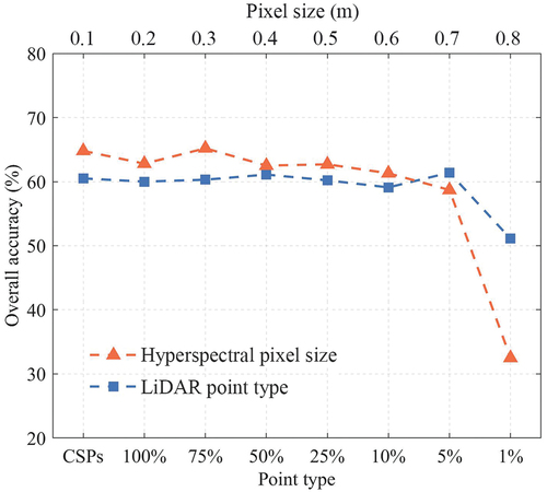
Figure 11 shows that the OA of CSPs was consistent with the original point cloud (100% density), as well as the 75%–5% density points (McNemar’s test, p > 0.05). When the point cloud density was reduced to 1%, the OA decreased rapidly by approximately 10%. For different hyperspectral spatial resolution images, the OA decreased significantly when the pixel size was larger than 0.3 m (McNemar’s test, p < 0.05). The OA dropped by approximately 30% when the spatial resolution was reduced to 0.8 m.

Figure 11. Classification results of the canopy surface points (CSPs), point clouds with different densities (100%–1%) and hyperspectral images with different spatial resolutions (0.1–0.8 m).

By comparing the features selected from CSPs and the original point clouds, we found that the H1, Hmad, RCD and CD_std were retained in the CSP classification (Supplementary Material Table S3). As the density of the point cloud decreased, the selected features hardly changed, except for features with a point density of 1%. When the density of points was less than 10%, the crown metrics and density variables were significantly different from the original point clouds. The hyperspectral features were less affected by the spatial resolution, especially the vegetation index (Supplementary Material Table S4).

4. Discussion

4.1 Contributions of ULS and UHSI features

Recently, the aggregate of advanced UAV and sensor techniques has been explored as an accurate means of characterizing forest structure at fine spatial/spectral scales. However, ULS and UHSI data with large amounts of spatial/spectral information also pose challenges for natural secondary forest species classification studies. In this study, we integrated ULS and UHSI data and performed comprehensive feature mining to discriminate 11 tree species in natural secondary forests. A total of 266 variables were extracted from ULS and UHSI data, comprehensively covering the geometric, radiometric, spectral and textural characteristics of trees. When using the same data sources, previous studies ignored the tree crown metrics (Cao et al. 2021; Qin et al. 2022). Herein, we implemented a rigorous and complete variable selection pipeline by combining a CFS and an optimized RFE algorithm. Compared to the studies by Zhou et al. (2022), we refitted the RF model and obtain a new importance ranking at each variable elimination. The results in this study indicated that after feature selection, using approximately 10 variables achieved a classification accuracy similar to that using approximately 30 variables (see Figure 6).

Based on the importance ranking of the selected features (Figure 9), we found that except for texture features and original band reflectance (b1-b96), other feature categories contributed significantly to classification. This might be because this study area is dominated by broad-leaved trees, and the texture characteristics of broad-leaved trees are similar, thus so they contribute less than spectral features, which is the same as the findings of Dan et al. (2015). The MNF components converted by the original band reflectance effectively represented the characteristics of the original band (Cao et al. 2021). Comparable to Yifang et al. (2018), we found that Imean_single ranked among the top few variables, illustrating that radiometric metrics are crucial in species classification. The Last_all_ratio was the second most important variable, and Ørka, Næsset, and Martin Bollandsås (2010) also reported the importance of the last returns for tree species discrimination. This finding implied that these two LiDAR variables represented the geometry structure characteristics of trees well. Moreover, the most important hyperspectral features were the VARI_red_edge, a structure-dependent vegetation index that was found to be virtually unaffected by atmospheric effects (Anatoly et al. 2002). We also found that the RVSI was important for classification, and identified inter- and intraspecies trends based on spectral changes in red-edge range (Merton 1999). This result is consistent with the results of Shi et al. (2018) and Qin et al. (2022). Additionally, 6 vegetation indices related to chlorophyll and carotenoid concentrations (DD, BGI, TCI, NPQI, NPCI and PRI) also made important contributions to tree species classification. Qin et al. (2022) and Run et al. (2021) also report the important role of PRI. Moreover, two crown metrics, including CD_std related to crown size and the RCD related to crown shape also showed optimistic importance. This demonstrated that crown morphological characteristics varied by tree species, and this difference was detected using LiDAR data. Run et al. (2021) also confirmed the important role of crown metrics in tree species detection.

Based on our results, we demonstrated that LiDAR and hyperspectral data combined can effectively increase the classification accuracy, which is in line with many early studies (Dian et al. 2016; Shi et al. 2018). This is mainly because the integration of LiDAR point clouds and hyperspectral images can provide both structural and spectral information. Similar to the study by Shi et al. (2018), we also found that hyperspectral features outperformed LiDAR features base on overall classification accuracy. One reason might be that the morphological differences among broad-leaved tree species are not as obvious as spectral differences. In this study, the OA of separating 11 tree species reached 75.7%, which was slightly inferior to that of some other studies; for instance, Shi et al. (2018) obtained 83.7% OA for discriminating five mixed temperate forest tree species, and Cao et al. (2021) obtained 97.22% OA for classifying seven mangrove tree species. However, Qin et al. (2022) mentioned that the increase in tree species has a negative impact on classification accuracy, we achieved high accuracy when faced with multispecies classification. For example, Liu et al. (2017) obtained a 70.0% OA when mapping 15 common urban tree species, and Zhong et al. (2020) discriminated eight tree species and obtained a 66.34% OA in a subtropical natural forest in southwest China. The accuracy of the broad leaf species F.M. and J.M. and the conifer species L.O. and P.K. were all over 85%. Overall, we achieved a reasonable accuracy using advanced ULS and UHSI for individual tree species classification in typical natural secondary forests.

4.2 Robustness and transferability of features

The greatest value of UAV in forest resource surveys is its repeatable operation (Hao et al. 2022). Therefore, the re-use of UAV features deserves attention. Yifang et al. (2018) evaluated the robustness and transferability of the RF model and selected LiDAR features in two study sites. However, limited by the cost of data acquisition, most studies use only a single study area, and due to the specificity of UAV systems and the subjectivity of flight parameters, it is difficult to directly transplant UAV-derived features to other study areas (Rana et al. 2022). To overcome this, it is common practice to use point clouds with different densities and images with different spatial resolutions to test the transferability of models or features. This study additionally employed canopy surface points to evaluate the performance of features, which provides a detailed reference on how to balance cost and efficiency when UAVs are re-used. The results showed that even if the features used were not exactly the same as the original point cloud features, tree species classification with CSPs produced comparable accuracies. Although Ghanbari Parmehr and Amati (2021) believed that photogrammetry point clouds and LiDAR point clouds were highly consistent, that may be due to their study area was located in an extremely sparse forest. The comparable classification accuracy produced by CSPs proved that structural differences in the canopy surface have the ability to discriminate tree species. Yifang et al. (2018) also pointed out that crown top layer is the main source of structural differences between tree species. Features of CSPs are not affected by the penetration properties of the sensor and are more robust when using different types of scan data. In future UAV applications, lower cost photogrammetric point clouds similar to CSPs can be considered for tree species identification, but due to the lack of intensity and echo-related information of photogrammetric point clouds, perhaps a leaf-off condition of a low-density forest is more suitable for it (Liu et al. 2021).

For the resampled LiDAR data, the selected features were robust from 100% (104.43 pts/m²) to 25% (26.11 pts/m²) of the original point cloud density. Almost none of the crown metrics could be extracted when the point cloud density was less than 10% (10.44 pts/m²). However, even a 5% density (5.22 pts/m²) point cloud resulted in classification accuracy comparable to that of the original data. Since the point cloud density is affected by flight altitude and speed, an appropriate data density is one to which practitioners pay close attention. Wang et al. (2022) also demonstrated that the classification accuracies and feature selection were minimally affected by point density. Since features at different resolutions were all computed based on the mean of the crown object, hyperspectral features were hardly affected. However, as the resolution decreased, the details of the tree crown were lost, and the contribution of some features was weakened, resulting an influence on the classification accuracy. This result also demonstrated the value of high-resolution data in tree species classification. Although we did not resample the spectral bands by design, five VIs retained in this study were associated with the multispectral red, blue, green, and red-edge bands (GI, VARI, BGI, NPCI, PRI). Zhong et al. (2020) similarly demonstrated the importance of the GI feature when using multispectral data for tree species discrimination. In summary, the feature selection results and classification results of resampled data and CSPs demonstrated the robustness of selected ULS and UHSI features and the potential for applicability in other study areas.

4.3 Limitations and future work

In addition to the data sources explored above, the accuracy of UAV-assisted tree species discrimination is affected by many factors, such as the size of samples, individual tree segmentation, canopy shading and soil background effects (Ruiliang 2021). In this study, the RF classifier was used to overcome the problem of unbalanced sample size (Hartling, Sagan, and Maimaitijiang 2021), and the results showed that some small samples of species such as L.O. and P.K. achieved satisfactory classification accuracy. However, misclassification still occurred for some tree species, such as P. A., A.M. and T.I. In addition to the effect of the small sample size, this is probably due to the similarities in spectra and morphology of different species, and variability within the same tree species. These variations may be due to differences in stand conditions (such as temperature, soil condition or topography), as well as tree competition, which introduces additional uncertainties in the classification (Yifang et al. 2018). In this study, trees were recorded at trunk locations, but they were identified based on the UAV view of the canopy, which may have led to errors when matching the measured trees with the detected trees. Additionally, due to overlapping crowns of adjacent trees, inaccurate tree segmentation leads to loss of crown architecture. Although we manually corrected the point clouds of samples, improving the efficiency and accuracy of tree segmentation in natural secondary forests for greater classification accuracy is still a potential topic for future research. In this study, the soil background mask on CHM was extracted with a threshold of 4 m during tree segmentation, and the thresholds of NIR and NDVI were set to filter the shadows inside the crown during object-oriented hyperspectral feature extraction, which was similar to the approach used by Piiroinen et al. (2018).

This study site adequately represents the ecological conditions and environmental settings of the Maoershan Forest Farm, and includes the vast majority of tree species in the northeast. It can be generalized in similar natural secondary forests in northeast China. Further experiments can be conducted again in other types of forests in the future. In addition, leaf-on/off data in different seasons can be integrated to explore changes in tree features across the phenological period to improve species classification accuracy. Collecting more samples and exploring deep learning models that do not rely on feature selection to improve classification accuracy are also future research goals.

5. Conclusions

In this study, we extracted hundreds of structural and reflective/radiative variables using ULS and UHSI data and screened the optimal subset of features for classifying 11 common tree species in typical natural secondary forests. The results demonstrated that the combination of ULS and UHSI effectively improved tree species discrimination accuracy compared to using either of them alone (OA increased by 15.7% and 10.9%, respectively). The mean intensity of single returns and the visible atmospherically resistant index for red-edge band were the most influential LiDAR and hyperspectral derived features, respectively. A simulation application showed that our selected features have good robustness in point clouds with different densities and images with different spatial resolutions. When using LiDAR for tree species classification, the point cloud density is recommended no less than 5 pts/m², and the canopy surface points are also a good choice and when using hyperspectral data, the spatial resolution recommends not to be lower than 0.3 m. This study provides a comprehensive feature mining and tree species discrimination pipeline using ULS and UHSI data and demonstrates the potential transferability of UAV data-assisted tree species classification in other study areas.

Acknowledgements

This research was supported by the National Key R&D Program of China (grant number 2020YFC1511603); Fundamental Research Funds for the Central Universities (grant number 2572020BA07).

Disclosure statement

No potential conflict of interest was reported by the author(s).

Data availability statement

The data that support the findings of this study are available from the corresponding author, (M.L), upon reasonable request (https://forestry.nefu.edu.cn/info/1038/1531.htm).

Supplementary material

Supplemental data for this article can be accessed online at https://doi.org/10.1080/15481603.2023.2171706

Additional information

Funding

The work was supported by the Fundamental Research Funds for the Central Universities [2572020BA07]; National Key Research and Development Program of China [2020YFC1511603].

References

- Adão, T., J. Hruška, L. Pádua, J. Bessa, E. Peres, R. Morais, and J. João Sousa. 2017. “Hyperspectral Imaging: A Review on UAV-Based Sensors, Data Processing and Applications for Agriculture and Forestry.” Remote Sensing 9 (11): 1110. doi:10.3390/rs9111110.
- Ali, A. M., R. Darvishzadeh, A. K. Skidmore, and I. van Duren. 2017. “Specific leaf area estimation from leaf and canopy reflectance through optimization and validation of vegetation indices“. Agricultural and Forest Meteorology 236: 162–17.
- Anatoly, G., J. Y. Kaufman, R. Stark, and D. Rundquist. 2002. “Novel Algorithms for Remote Estimation of Vegetation Fraction.“ Remote Sensing of Environment 80 (1): 76–87.
- Asner, G. P. 1998. “Biophysical and Biochemical Sources of Variability in Canopy Reflectance.“ Remote Sensing of Environment 64 (3): 234–253.
- Belgiu, M., and L. Drăgu. 2016. “Random Forest in Remote Sensing: A Review of Applications and Future Directions.” Isprs Journal of Photogrammetry and Remote Sensing 114: 24–31. doi:10.1016/j.isprsjprs.2016.01.011.
- Bergstra, J., C. James, and C. Yoshua. 2012. “Random Search for Hyper-Parameter Optimization Yoshua Bengio.” Journal of Machine Learning Research 13: 281–305.
- Boerema, A., A. J. Rebelo, M. B. Bodi, K. J. Esler, and P. Meire. 2017. “Are Ecosystem Services Adequately Quantified?” The Journal of Applied Ecology 54 (2): 358–370. doi:10.1111/1365-2664.12696.
- Breiman, L. 2001. “Random Forests.” Machine Learning 45 (1): 5–32. doi:10.1023/A:1010933404324.
- Cao, J., K. Liu, L. Zhuo, L. Liu, Y. Zhu, and L. Peng. 2021. “Combining UAV-Based Hyperspectral and LiDar Data for Mangrove Species Classification Using the Rotation Forest Algorithm.” International Journal of Applied Earth Observation and Geoinformation 102: 102414. doi:10.1016/j.jag.2021.102414.
- Cazzolla Gatti, R., P. B. Reich, J. G. P. Gamarra, T. Crowther, C. Hui, A. Morera, J. F. Bastin, et al. 2022. “The Number of Tree Species on Earth.” Proceedings of the National Academy of Sciences of the United States of America 119 (6). doi:10.1073/pnas.2115329119.
- Clark, M. L., and D. A. Roberts. 2012. Remote Sensing Species-Level Differences in Hyperspectral Metrics Among Tropical Rainforest Trees as Determined by a Tree-Based Classifier. In, 1821, 4(6): 1820–1855. 10.3390/rs4061820.
- Colomina, I., and P. Molina. 2014. “Unmanned Aerial Systems for Photogrammetry and Remote Sensing: A Review.”ISPRS Journal of Photogrammetry and Remote Sensing 92: 79–97.
- Coops, N. C., T. Hilker, M. A. Wulder, B. St-Onge, G. Newnham, A. Siggins, and J. A. Trofymow. 2007. “Estimating Canopy Structure of Douglas-Fir Forest Stands from Discrete-Return LiDar.” Trees - Structure and Function 21 (3): 295–310. doi:10.1007/s00468-006-0119-6.
- Dalponte, M., L. Bruzzone, and D. Gianelle. 2012. “Tree Species Classification in the Southern Alps Based on the Fusion of Very High Geometrical Resolution Multispectral/Hyperspectral Images and LiDar Data.” Remote Sensing of Environment 123: 258–270.
- Dan, L., K. Yinghai, H. Gong, and L. Xiaojuan. 2015. “Object-Based Urban Tree Species Classification Using Bi-Temporal WorldView-2 and WorldView-3 Images.” Remote Sensing 7 (12): 16917–16937. doi:10.3390/rs71215861.
- Dian, Y., Y. Pang, Y. Dong, and L. Zengyuan. 2016. “Urban Tree Species Mapping Using Airborne LiDar and Hyperspectral Data.” Journal of the Indian Society of Remote Sensing 44 (4): 595–603. doi:10.1007/s12524-015-0543-4.
- Fassnacht, F. E., H. Latifi, K. Stereńczak, A. Modzelewska, M. Lefsky, L. T. Waser, C. Straub, and A. Ghosh. 2016. “Review of Studies on Tree Species Classification from Remotely Sensed Data.” Remote sensing of environment 186: 64–87. doi:10.1016/j.rse.2016.08.013.
- Fricker, G. A., J. A. Wolf, S. S. Saatchi, and T. W. Gillespie. 2015. “Predicting Spatial Variations of Tree Species Richness in Tropical Forests from High-Resolution Remote Sensing.” Ecological Applications 25 (7): 1776–1789. doi:10.1890/14-1593.1.
- Gao, H., B. Huiquan, and L. Fengri. 2017. “Modelling Conifer Crown Profiles as Nonlinear Conditional Quantiles: An Example with Planted Korean Pine in Northeast China.” Forest Ecology and Management 398: 101–115. doi:10.1016/j.foreco.2017.04.044.
- Ghanbari Parmehr, E., and M. Amati. 2021. “Individual Tree Canopy Parameters Estimation Using UAV-Based Photogrammetric and LiDar Point Clouds in an Urban Park.” Remote Sensing 13 (11). doi:10.3390/rs13112062.
- Goodbody, T. R. H., N. C. Coops, P. L. Marshall, P. Tompalski, and P. Crawford. 2017. “Unmanned Aerial Systems for Precision Forest Inventory Purposes: A Review and Case Study.” The Forestry Chronicle 93 (01): 71–81.
- Green, A. A., M. Berman, P. Switzer, and M. D. Craig. 1988. “A Transformation for Ordering Multispectral Data in Terms of Image Quality with Implications for Noise Removal.“ IEEE Transactions on Geoscience and Remote Sensing 26 (1): 65–74.
- Gregorutti, B., B. Michel, and P. Saint-Pierre. 2017. “Correlation and Variable Importance in Random Forests.” Statistics and Computing 27 (3): 659–678. doi:10.1007/s11222-016-9646-1.
- Guo, Q., L. Wenkal, Y. Hong, and O. Alvarez. 2010. “Effects of Topographie Variability and Lidar Sampling Density on Several DEM Interpolation Methods.” Photogrammetric Engineering and Remote Sensing 76 (6): 701–712. doi:10.14358/PERS.76.6.701.
- Hao, Y., F. Rafi Almay Widagdo, X. Liu, Y. Quan, Z. Liu, L. Dong, and L. Fengri. 2022. “Estimation and Calibration of Stem Diameter Distribution Using UAV Laser Scanning Data: A Case Study for Larch (Larix Olgensis) Forests in Northeast China .“ Remote Sensing of Environment 268: 112769.
- Hao, Y., Z. Zhen, L. Fengri, and Y. Zhao. 2019. “A Graph-Based Progressive Morphological Filtering (GPMF) Method for Generating Canopy Height Models Using ALS Data.” International Journal of Applied Earth Observation and Geoinformation 79: 84–96.
- Hartling, S., V. Sagan, and M. Maimaitijiang. 2021. “Urban Tree Species Classification Using UAV-Based Multi-Sensor Data Fusion and Machine Learning.” GIScience & Remote Sensing 58 (8): 1250–1275. doi:10.1080/15481603.2021.1974275.
- Kirby, K. R., and C. Potvin. 2007. “Variation in Carbon Storage Among Tree Species: Implications for the Management of a Small-Scale Carbon Sink Project.” Forest Ecology and Management 246 (2–3): 208–221. doi:10.1016/j.foreco.2007.03.072.
- Korpela, I. S., and T. Erkki Tokola. 2006. “Potential of Aerial Image-Based Monoscopic and Multiview Single-Tree Forest Inventory: A Simulation Approach.“ Forest Science 52 (2): 136–147.
- Korpela, I., H. Ole Ørka, M. Maltamo, T. Tokola, and J. Hyyppä. 2010. “Tree Species Classification Using Airborne LiDar – Effects of Stand and Tree Parameters, Downsizing of Training Set, Intensity Normalization, and Sensor Type.” Silva Fennica 44 (2): 319–339. doi:10.14214/sf.156.
- Liu, L., N. C. Coops, N. W. Aven, and Y. Pang. 2017. “Mapping Urban Tree Species Using Integrated Airborne Hyperspectral and LiDar Remote Sensing Data.” Remote Sensing of Environment 200: 170–182.
- Liu, K., A. Wang, S. Zhang, Z. Zhu, B. Yufang, Y. Wang, and D. Xuhua. 2021. “Tree Species Diversity Mapping Using UAS-Based Digital Aerial Photogrammetry Point Clouds and Multispectral Imageries in a Subtropical Forest Invaded by Moso Bamboo (Phyllostachys Edulis).” International Journal of Applied Earth Observation and Geoinformation 104: 102587. doi:10.1016/j.jag.2021.102587.
- Masek, J. G., D. J. Hayes, M. Joseph Hughes, S. P. Healey, and D. P. Turner. 2015. “The Role of Remote Sensing in Process-Scaling Studies of Managed Forest Ecosystems.” Forest Ecology and Management 355 (1): 109–123.
- Mäyrä, J., S. Keski-Saari, S. Kivinen, T. Tanhuanpää, P. Hurskainen, P. Kullberg, L. Poikolainen, et al. 2021. “Tree Species Classification from Airborne Hyperspectral and LiDar Data Using 3D Convolutional Neural Networks.” Remote Sensing of Environment 256: 112322. doi:10.1016/j.rse.2021.112322.
- McNemar, Q. 1947. “Note on the Sampling Error of the Difference Between Correlated Proportions or Percentages.” In Psychometrika 12 (2): 153–157.
- Merton, R. 1999. “Monitoring Community Hysteresis Red-Edge Vegetation Stress Index.“ JPL Airborne Earth Science Workshop, NASA, Jet Propulsion Laboratory , Pasadena, California, USA.
- Michałowska, M., and J. Rapiński. 2021. “A Review of Tree Species Classification Based on Airborne Lidar Data and Applied Classifiers.” Remote Sensing 13 (3): 353.
- Ørka, H. O., M. Dalponte, T. Gobakken, E. Næsset, and L. Theodor Ene. 2013. “Characterizing Forest Species Composition Using Multiple Remote Sensing Data Sources and Inventory Approaches.” Scandinavian Journal of Forest Research 28 (7): 677–688.
- Ørka, H. O., E. Næsset, and O. Martin Bollandsås. 2010. “Effects of Different Sensors and Leaf-On and Leaf-Off Canopy Conditions on Echo Distributions and Individual Tree Properties Derived from Airborne Laser Scanning.” Remote Sensing of Environment 114(7): 1445–1461.
- Pal, M. 2005. “Random Forest Classifier for Remote Sensing Classification.” International Journal of Remote Sensing 26 (1): 217–222. doi:10.1080/01431160412331269698.
- Pedregosa, F., G. Varoquaux, A. Gramfort, V. Michel, B. Thirion, O. Grisel, S.L.M. Blondel, et al. 2011. Scikit-Learn: Machine Learning in Python. Paper presented at the J. Mach. Learn. Res.
- Piiroinen, R., F. Ewald Fassnacht, J. Heiskanen, E. Maeda, B. Mack, and P. Pellikka. 2018. “Invasive Tree Species Detection in the Eastern Arc Mountains Biodiversity Hotspot Using One Class Classification.” Remote sensing of environment 218: 119–131. doi:10.1016/j.rse.2018.09.018.
- Qin, H., W. Zhou, Y. Yao, and W. Wang. 2022. “Individual Tree Segmentation and Tree Species Classification in Subtropical Broadleaf Forests Using UAV-Based LiDar, Hyperspectral, and Ultrahigh-Resolution RGB Data.” Remote Sensing of Environment 280. doi:10.1016/j.rse.2022.113143.
- Quan, Y., L. Mingze, Y. Hao, and B. Wang. 2021. “Comparison and Evaluation of Different Pit-Filling Methods for Generating High Resolution Canopy Height Model Using Uav Laser Scanning Data.” Remote Sensing 13 (12): 2239. doi:10.3390/rs13122239.
- Quan, Y., L. Mingze, Z. Zhen, Y. Hao, and B. Wang. 2020. “The Feasibility of Modelling the Crown Profile of Larix Olgensis Using Unmanned Aerial Vehicle Laser Scanning Data.” Sensors (Switzerland) 20 (19): 1–20. doi:10.3390/s20195555.
- Rana, P., B. St-Onge, J. François Prieur, B. Cristina Budei, A. Tolvanen, and T. Tokola. 2022. “Effect of Feature Standardization on Reducing the Requirements of Field Samples for Individual Tree Species Classification Using ALS Data .” ISPRS Journal of Photogrammetry and Remote Sensing 184: 189–202.
- Ruiliang, P. 2021. “Mapping Tree Species Using Advanced Remote Sensing Technologies: A State-Of-The-Art Review and Perspective.” Journal of Remote Sensing 2021: 1–26. doi:10.34133/2021/9812624.
- Run, Y., Y. Luo, Q. Zhou, X. Zhang, W. Dewei, and L. Ren. 2021. “A Machine Learning Algorithm to Detect Pine Wilt Disease Using UAV-Based Hyperspectral Imagery and LiDar Data at the Tree Level.” International Journal of Applied Earth Observation and Geoinformation 101: 102363. doi:10.1016/j.jag.2021.102363.
- Schaepman-Strub, G., M. E. Schaepman, T. H. Painter, S. Dangel, and J. V. Martonchik. 2006. “Reflectance Quantities in Optical Remote Sensing—definitions and Case Studies.” Remote sensing of environment 103 (1): 27–42. doi:10.1016/j.rse.2006.03.002.
- Schiefer, F., T. Kattenborn, A. Frick, J. Frey, P. Schall, B. Koch, and S. Schmidtlein. 2020. “Mapping Forest Tree Species in High Resolution UAV-Based RGB-Imagery by Means of Convolutional Neural Networks.” ISPRS Journal of Photogrammetry and Remote Sensing 170: 205–215.
- Shi, Y., A. K. Skidmore, T. Wang, S. Holzwarth, U. Heiden, N. Pinnel, X. Zhu, and M. Heurich. 2018. “Tree Species Classification Using Plant Functional Traits from LiDar and Hyperspectral Data.” International Journal of Applied Earth Observation and Geoinformation 73: 207–219.
- van Aardt, J. A. N., and R. H. Wynne. 2007. “Examining Pine Spectral Separability Using Hyperspectral Data from an Airborne Sensor: An Extension of Field-Based Results.” International Journal of Remote Sensing 28 (2): 431–436. doi:10.1080/01431160500444772.
- Wai Tim, N., P. Rima, K. Einzmann, M. Immitzer, C. Atzberger, and S. Eckert. 2017. “Assessing the Potential of Sentinel-2 and Pléiades Data for the Detection of Prosopis and Vachellia Spp. In Kenya.” Remote Sensing 9 (1): 74. doi:10.3390/rs9010074.
- Wang, D., B. Wan, Q. Penghua, T. Xiang, and Z. Quanfa. 2022. “Mapping Mangrove Species Using Combined UAV-LiDar and Sentinel-2 Data: Feature Selection and Point Density Effects.” Advances in Space Research 69 (3): 1494–1512.
- Yifang, S., T. Wang, A. K. Skidmore, and M. Heurich. 2018. “Important LiDar Metrics for Discriminating Forest Tree Species in Central Europe.” Isprs Journal of Photogrammetry and Remote Sensing 137: 163–174. doi:10.1016/j.isprsjprs.2018.02.002.
- Yinghui, Z., Y. Ma, L. J. Quackenbush, and Z. Zhen. 2022. “Estimation of Individual Tree Biomass in Natural Secondary Forests Based on ALS Data and WorldView-3 Imagery.” Remote Sensing 14 (2): 271. doi:10.3390/rs14020271.
- Zhang, L., L. Dong, Q. Liu, and Z. Liu. 2020. “Spatial Patterns and Interspecific Associations During Natural Regeneration in Three Types of Secondary Forest in the Central Part of the Greater Khingan Mountains, Heilongjiang Province, China.” Forests 11 (2): 152. doi:10.3390/f11020152.
- Zhang, B., L. Zhao, and X. Zhang. 2020. “Three-Dimensional Convolutional Neural Network Model for Tree Species Classification Using Airborne Hyperspectral Images.” Remote Sensing of Environment 247: 111938.
- Zhao, Y., Y. Hao, Z. Zhen, and Y. Quan. 2017. “A Region-Based Hierarchical Cross-Section Analysis for Individual Tree Crown Delineation Using ALS Data.” Remote Sensing 9 (10): 1084. doi:10.3390/rs9101084.
- Zhen, Z., L. Yang, Y. Ma, Q. Wei, H. Il Jin, and Y. Zhao. 2022. “Upscaling Aboveground Biomass of Larch (Larix Olgensis Henry) Plantations from Field to Satellite Measurements: A Comparison of Individual Tree-Based and Area-Based Approaches.” GIScience & Remote Sensing 59 (1): 722–743. doi:10.1080/15481603.2022.2055381.
- Zhong, X., X. Shen, L. Cao, N. C. Coops, T. R. H. Goodbody, T. Zhong, W. Zhao, et al. 2020. “Tree Species Classification Using UAS-Based Digital Aerial Photogrammetry Point Clouds and Multispectral Imageries in Subtropical Natural Forests.“ International Journal of Applied Earth Observation and Geoinformation 92: 102173.
- Zhongya, Z., A. Kazakova, L. Monika Moskal, and D. M. Styers. 2016. “Object-Based Tree Species Classification in Urban Ecosystems Using LiDar and Hyperspectral Data.” Forests 7 (12): 1–16. doi:10.3390/f7060122.
- Zhou, K., L. Cao, H. Liu, Z. Zhang, G. Wang, and F. Cao. 2022. “Estimation of Volume Resources for Planted Forests Using an Advanced LiDar and Hyperspectral Remote Sensing.” Resources, Conservation & Recycling 185:106485.