Using remote sensing for exposure and seismic vulnerability evaluation: is it reliable?

ABSTRACT

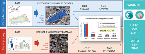
Conducting field surveys for exposure and seismic vulnerability evaluation is the most costly, resource-intensive task when assessing earthquake risk. During the past decade, risk analysts have been trying to alleviate this using remote sensing for building characterization. However, the use of vulnerability databases created with remote sensing had not been sufficiently validated thus far. In this paper, we have created an exposure and seismic vulnerability database in Port Prince (Haiti) using freely accessible aerial ortho-imagery and LiDAR points. We have validated this database against two reference datasets from different, independent studies. Then, we have computed an earthquake damage scenario to test whether remotely sensed data are actually valid for seismic risk evaluation. We have seen how our vulnerability database yields an accurate damage distribution with a low Mean Absolute Percentage Error of 3.78% when compared to the damage obtained with the reference vulnerability dataset. Further, we have conducted a thorough comparison of the cost that entails creating a vulnerability database using remote sensing with a traditional field survey. Twelve international experts have collaborated in the cost estimation of a typical in-field building inspection. As a result, we have found that using remote sensing techniques allows for saving up to 75% of the cost and 85% of the time. These outcomes seem to prove both, the technical and economic feasibility of remote sensing for seismic vulnerability assessment. Thus, we have proposed a 5-step approach for evaluating building vulnerability that combines both, the analysis of remotely sensed data and a reduced, targeted field survey to optimize time and cost. The final goal is to help cities reach the Sustainable Development Goal nr. 11.B to increase their resilience against disasters.

GRAPHICAL ABSTRACT

KEYWORDS:

• Remote sensing
• LiDAR
• seismic vulnerability
• earthquake damage
• field survey optimization

Introduction

More than half the fatalities caused by natural disasters over the last 20 years were earthquake-related. The report published by CRED, UNISDR (2016) on the natural disasters that struck between 1996 and 2015 underlines the fact that the overwhelming majority of these victims lived in developing countries. In the Sendai Framework, the UN set out to promote the implementation of disaster risk reduction (DRR) measures, primarily for two reasons: (1) the frequency and deadliness of natural disasters have increased over the years; and (2) estimates indicate that urban areas are becoming increasingly vulnerable. As a matter of fact, the Sustainable Development Goal (SDG) nr. 11.B seeks to increase the resilience of cities and communities to disasters (SDG-United Nations).

Of the seven global objectives established in the Sendai Framework, three are worth highlighting as especially relevant to the present study: (1) expanding the number of countries implementing DRR strategies by 2020; (2) implementing sustainable actions to enhance international cooperation on this matter in developing countries; and (3) making multi-hazard systems and disaster-risk data more widely available and accessible to the general population.

It seems clear that we need to learn about these natural hazards to protect ourselves from them. In the case of earthquakes, assessing the seismic risk in an area entails evaluating the hazard and characterizing the building stock. This paper focuses on the latter, known as exposure and vulnerability assessment. The process was structured in three key steps. The first step was identifying the most typical building typologies in the city’s building stock. The next step consisted of gathering as much relevant seismic vulnerability information as possible about every building in the study city. All this information was stored as attributes and used to generate the exposure database. Based on these attributes, the buildings were classified according to the typologies identified in the previous step. Finally, each category mentioned above was assigned a vulnerability model that indicates how each typology will behave in the event of an earthquake.

In its Global Assessment Report (GAR 2009), the UN states that, in addition to nature’s inherent unpredictability, data constraints make it challenging to understand risk. Because data is not always available, up-to-date, or duly disaggregated, analysts are forced to generate data from scratch in most cases. Traditionally, data collection is carried out through in-field campaigns in which a group of engineers and architects specializing in seismic vulnerability go around the city collecting data about buildings and other structures of interest. This task is arduous, resource-intensive, and time-consuming (e.g. Zhou et al. 2022). Consequently, creating and maintaining exposure databases has become a challenge for cities with a medium-high seismic risk.

The main objective of the present paper is to take steps toward exploiting available data to optimize the processes of understanding and characterizing seismic vulnerability in urban environments using remote sensing and machine learning. Moreover, we will evaluate the technical and economic feasibility of using this data in a seismic damage assessment.

Over the past two decades, numerous studies have been successfully conducted that focused on incorporating the use of remote sensing to evaluate, not only disaster damage (e.g. Moya et al. 2021; Stepinac and Gasparovic 2020; Corbane et al. 2011), but also exposure and seismic vulnerability (e.g. Fan et al. 2021; Wieland et al. 2012, 2012). Nevertheless, certain issues have yet to be addressed: robust validation, data-fusion strategy, economic analysis or cost/benefit evaluation, and applicability in a complete damage assessment. The present paper aims to address these aspects through a comprehensive study in which we have: created an exposure and vulnerability database using remotely sensed data and machine learning techniques for Port Prince (Haiti); conducted a thorough analysis of uncertainties; contrasted this database with ground truth to conduct a damage assessment, and compared the cost of generating this database with the actual cost of an in-field survey used to create a comparable product. Finally, we propose a procedure for creating an exposure and vulnerability database by combining the two data-capture methods.

The present article is structured as follows: Section 2 presents a literature review of studies devoted to seismic vulnerability evaluation using remote sensing. Sections 3 describes the study area, the data, and the methodological framework. Section 4 presents the calculation of the exposure and vulnerability database, as well as the feasibility analysis. The conclusions are presented in Section 5.

Background: exposure and vulnerability evaluation using remote sensing

The study presented herein is the last part of a series of previous related studies that we have been carrying out since the 2010 earthquake in Haiti. In Molina et al. (2014) and Torres et al. (2016), we conducted an in-field survey in Port Prince to study the city’s building stock. By integrating this data with a newly compiled cadastral database provided by the Haitian Ministry of Public Works, we conducted an initial seismic risk study. The new techniques for assessing seismic vulnerability based on remote sensing and machine learning were first introduced in Wieland et al. (2016). Yolanda et al. (2019) presented a complete, parallel application conducted in the Spanish city of Lorca. The present paper offers a final comprehensive step in which earthquake damage is accurately evaluated using a vulnerability database created with data gathered using only remote sensing and machine learning.

Table 1 presents a structured summary of the most relevant studies carried out over the past 15 years to detect buildings and evaluate earthquake exposure and/or vulnerability using in-field surveys, remote sensing, and ancillary data. The table builds upon the tables presented in Guiwu et al. (2015) and Wenhua et al. (2017).

Table 1. Comparative overview of studies aimed at evaluating seismic vulnerability using remote sensing data. The studies are divided according to the type of data they use: optical imagery, 3D data and other information.

Author	Data	Comments to the main topics addressed	Accuracy or reliability
Optical imagery
Wieland et al. (2012)	Time-series of Landsat TM and MSS; QuickBird; manual digitization.	Age of construction from Landsat time series analysis. LULC classification from OBIA of Landsat image. QuickBird image analysis for footprint delineation: segmentation + post-processing for over-segmentation solution + SVM for classification. Testing built-up mask with 5964 manually digitized buildings; testing MBT with 15,098 manually digitized buildings.	Accuracy of OBIA of Landsat is 81%. Footprints from QuickBird (built-up mask): Accuracy = 90%.
Dell’acqua, Gamba, and Jaiswal (2013)	QuickBird image.	Design of BREC-4-GEM software for extracting the number of buildings.	Buildings are detected with accuracy around 90%.
Ehrlich et al. (2013)	QuickBird image; DB of damage assessment after the Haiti 2010 EQ; Ground truth footprint DB provided by the municipality.	Alpha-tree of multi-level segmentations. Building segments were selected using parameters related to shape, area, width, length, spectral rage and presence of shadow. Height from shadow.	Sana’s: 78.86% of accuracy in built-up mask generation. Height not validated. Port Prince: nr. bldgs. estimated with R^2 = 0.64.
Shunping, Wei, and Meng (2019)	Aerial imagery with 0.075 m resolution and satellite imagery with 2.7 m resolution. Buildings manually delineated from various satellite images with resolution between 0.3–2.5 m.	Comparison of various Convolutional Neural Network-based methods for building detection and proposal of a new one: Siamese U-Net with shared weights in two branches. Used aerial dataset (130000 buildings for training; from which 14,500 are left for validation; 42000 for testing) and satellite dataset (21556 buildings for training, manually delineated; 7529 for testing).	Training with aerial data: IoU = 88.4; Recall = 93.9; Prec = 93.8. Validation in satellite data: IoU = (59.5–61.1); Recall = (78.0–79.6); Prec = (71.6–72.5).
Fan et al. (2021)	Images: MODIS (GSD 250–1000 m); Landsat OLI-8 (GSD 30 m); VIIRS Night Time Light (450 m).	Use of Support Vector Regression and random forest to estimate seismic vulnerability at pixel level. 15 features used in 391 pixel-level samples.	RMSE of vulnerability at pixel level~0.11 in training phase. Not tested with unseen data.
Optical imagery and 3D data
Panagiota et al. (2012)	VHR panchromatic image; DSM; building DB from in-field survey; footprints available.	Roof type (flat/gable) from panchromatic band and DEM with already existing footprints. Building height using DSM and footprints already available. Dataset with 1875 buildings.	Correlation between estimated vulnerability and ground truth data is 75%.
Polli and Dell’acqua (2011)	QuickBird panchromatic band; SAR.	W-filter for footprint extraction from image. Analysis of two SAR images of the same building for height extraction.	Not mentioned
Mueck et al. (2013)	QuickBird image; DEM from Radar; building DB from in-field survey; manual digitization.	QuickBird for OBIA and building extraction; DEM for height. Building vulnerability to earthquake and tsunami hazards is considered. Digitized 520 bldgs. for footprint verification.	Accuracy of footprint comparison is 84%. Building classification in testing phase: accuracy = 81%
Wieland et al. (2012); Pittore and Wieland (2013)	Time-series of Landsat images; ground-based omnidirectional imaging; OSM footprints; building DB from in-field survey; manual digitization.	OBIA of images for extracting building data at both, block and building levels. Height is extracted from 360º images. Nr. buildings estimated through the building density per stratum. Around 900 buildings for MBT verification.	Accuracy of OBIA of built-up mask creation ranges between 80%-90%. Validation of height is not provided. Validation of MBT classification is only visual.
Geiss et al. (2015)	IKONOS VNIR; Time-series of Landsat TM and ETM+; nDSM from Radar; vulnerability/damage DB from in-field survey. Vulnerability/damage DB from in-field survey of 3896 bldgs.	Calculation of features at both, building and block level. Multi-temporal analysis of Landsat images to extract the period of construction. Vulnerability allocation is done following (1) a scoring method (expert knowledge), (2) the EMS-98 scale, and (3) MBT definition. Damage calculation is performed using fragility functions derived with data from the 2009 earthquake.	(1) Vulnerability based on scoring: MAPE = 10.6%. When compared with (2) EMS-98, accuracy = 65.4% and kappa = 0.36 For (3) MBT classification, only visual validation is done for the 561 bldgs. The remaining 2221 bldgs. are validated by searching within a radius of 50 m, with accuracy = 84%. Damage is not validated.
Riedel et al. (2014, 2015)	Aerial images; DEM from airborne data; footprints from Cadaster; building DB from in-field survey with 3860 buildings; INSEE database with 6214 buildings.	Vulnerability proxy developed with the vulnerability DB. Calculation of 15 morphological indicators using cadastral data (footprints) and Remote Sensing. Two predictive models created (1) with all the attr., and (2) with only 2 attr., i.e. nr. stories and date, since these are the attr. present in the INSEE DB. Estimation of vulnerability is extended to the whole country using the INSEE French DB. A damage estimation is done and compared to a reference from the Risk-UE project.	Accuracy in training phase is 62.4% when only date and nr. stories are used. Maximum accuracy in training phase is 94.5% when all attr. are included. and the 6 vulnerability classes are merged into 3. Accuracy is not provided for the MBT classification of the entire French territory. Accuracy of the damage comparison is not quantified.
Costanzo et al. (2016)	LiDAR and IPERGEO 503-band VNIR images; cadastral data for verification.	DTM and DSM, together with image classification to characterize terrain, buildings and road network.	Roof type classification in testing phase: accuracy = 95% and kappa = 0.92. The rest is not validated.
Geiss et al. (2016)	RapidEye RGB-NIR images; DEM from TanDEM-X; Time series of Landsat; Expected damage DB; GPS-photos from Google Panoramio.	Multi-temporal analysis of Landsat images to extract the period of construction. Multi-scale segmentation to delineate the urban structures. Direct estimation of damage grades with predictive modeling and training dataset sizes from 145 to 582. The analysis is performed at an aggregated urban level, not at building level.	Accuracy of 3 urban structures classification is 85.6%, and kappa = 0.77. MAPE of damage assessment is 13%.
Geiss et al. (2017)	WorldView 2 RGB+NIR; OSM complete DB.	Multi-level segmentation and LULC classification with and 600 samples per class (6 classes). Integrated samples from OSM. An empirical relation between the nr. buildings in OSM and the segments classified as buildings is calculated for nr. building estimation. Testing DB with 1056 segments.	LULC classification accuracy is 86.7% with kappa = 0.81. MAPE of the best Nr. bldg. estimation is 26.21%.
Bittner et al. (2018)	WorldView 2 RGB + Panchromatic band; nDSM.	Building detection using a Fully Convolutional Network (FCN) with 3 different configurations of the network layers. Training dataset: 22057 patches; testing dataset: 3358 patches; both of 300 × 300 pixels.	Binary built-up mask: F-score training between 75.1% − 86.1%. F-score testing = 81%.
Yongyang et al. (2018)	ISPRS open datasets: Vaihingen: (IR+R+G+nDSM) 33 images with 9 cm resolution (16 tiles for ground-truth). Potsdam: (IR+R+G+B+nDSM) 38 images with 5 cm resolution (24 tiles for ground-truth).	Design of an image segmentation neural network based on the deep residual networks and uses a guided filter to extract buildings. Use of edge enhancement effect in pre-processing. Each dataset is split 80% − 20% for training and testing.	Building detection F1-score is 93.9% in Potsdam; and 95.1% in Vaihingen.
Liuzzi et al. (2019)	Airborne orthophoto RGB+NIR of 50 cm resolution. Building height is taken from the reference database.	Random Forest and K-Nearest Neighbors for building detection. Reference database: 13 819 masonry and 3 643 RC buildings from an in-field survey with actual footprints.	Training phase: Best model with Random Forest: F1-score = (92% −93%) Testing phase: F1-score = (56% − 65%) and Overall accuracy = (60% − 80%), Kappa = (0.20–0.31).
De Los Santos and Principe (2021)	nDSM from LiDAR and images.	Building footprints using image thresholding and classification of the nDSM. Does not perform well in densely populated areas. 2125 buildings extracted. MBT were then classified using 158 samples with SVM, RF and logistic reg.	F1-score of MBT prediction in training phase ranges between 53% − 78%. Not tested in unseen data.
Zhou et al. (2022)	UAV images of 2.3 cm GSD. RGB bands. nDSM from UAV oblique photogrammetry.	Building footprint and floor area estimation using five structures of convolutional neural networks. Applied in rural area (regular, compact building footprints). Dataset of 4980 images (70% for training, 30% for testing).	Building footprint extraction: F1 = 0.92; Building height: Acc = 94% (only 17 testing samples).
Optical imagery, 3D data and other useful information
Sarabandi et al. (2008)	QuickBird images; Tax assessor database; building DBs from in-field surveys; manual digitization.	Rational Polynomial Coefficients (RPC) are used to obtain the building height by measuring the image coordinates of the ground and roof points of a building corner. Sample: 23 bldgs. Footprint digitization for extraction of geometric and shape-related attributes. Two datasets with 38,135 and 1947 buildings, respectively.	Accuracy of height extraction by comparison with independent data survey: MAPE = 1.42%. Accuracy in testing phase for 6 MBT classification ranges between 63% − 84%.
Borfecchia et al. (2010)	LiDAR; AISA-Eagle RGB-NIR images Landsat ETM+; QuickBird; building DB from in-field survey; census data.	Footprints from local cartography 1:2000. LiDAR for nr. stories. AISA-Eagle images RGB-NIR for spectral signatures of roof inside the footprints. Landsat ETM+ and QuickBird images to obtain the date of construction (> or<2000) for RC buildings. In-field DB contains 233 bldgs. (60 for training and 173 for testing). Used Artificial Neural Networks, KNN and Decision Trees for MBT classification.	Accuracy of built-up areas: before 2000 is 84.5%; after 2000 is 70.5%. Accuracy in testing phase for 3 MBT classification is 85%. If RC classes are grouped, then accuracy for 2 MBT is 90%.
Hao et al. (2014)	WorldView-2 images; building DB from in-field survey; vulnerability database.	OBIA for building detection (shape and shadow). Height extracted from shadow for 48 isolated buildings.	Bldg. detection accuracy from OBIA is 81%. Height error<2 m.
Guiwu et al. (2015)	VHR Optical images; building-related local knowledge (Br-LK); DB from in-field survey with 954 buildings; manual digitization.	Digitization of footprints for area extraction. Algorithm for height extraction from optical images by measuring the building SIPD (shadow length). MBT classification using a simple rule based only on height.	MAPE of height is 3.23%. Estimated area is 2.99% lower than real. Accuracy of 3 MBT classification using rules is 96% and kappa = 0.88
Wenhua et al. (2017)	Google Earth images; Tencent/Baidu Street View; WeChat; VGI; Br-LK; Real state databases; institutional websites; local informants providing in-field data; manual digitization.	Improvement of previous study by Guiwu et al. (2015). For MBT classification, authors incorporate a great amount of information from internet sources and in-field informants in order to improve their previous accuracy. Exposure test DB (to verify area and height): 971 buildings. DB to verify structural type: 1016 buildings.	MAPE of area is 4.64%. Accuracy of nr. stories is 89% and kappa = 0.86 Accuracy of 3 MBT classification using rules is 98% and kappa = 0.94

Accuracy refers to global or overall accuracy. MAPE stands for Mean Absolute Percentage Error. MBT stands for Model Building Type, as a synonym of SBSTs (Seismic Building Structural Types). Abbreviations: attr. for attributes; bldgs. for buildings; DB for database. RC for reinforced concrete. EQ for earthquake. RF for Random Forest. SVM for Support Vector Machines.

When remote sensing is used to characterize the vulnerability of the urban environment, the first step is always to detect building footprints and generate a vector layer with them. These are then used to extract the remaining attributes. The footprints can be obtained from various sources. The first and most accurate are official maps, as in Borfecchia et al. (2010). Other existing maps, such as OpenStreetMap (Geiss et al. 2017) or Google Earth (Wenhua et al. 2017), can also be useful. If no footprints are available, these must be generated manually (Guiwu et al. 2015) or semi-automatically using image analysis and other spatial data (Wieland et al. 2012).

According to our experience, obtaining an accurate building footprint from the start is crucial to guaranteeing the accuracy of the rest of the study. Studies in which the footprint is extracted using semi-automated methods rarely provide a high degree of accuracy in their final results (see Table 1). This is why some authors make a case for using manual digitization to create building footprints (Wenhua et al. 2017). Although this method is rudimentary, it has proven to be fast and accurate. Nevertheless, it is not scalable to large regions. The present paper compares the final results obtained with manually digitized footprints and semi-automated extraction using high-resolution aerial imagery and LiDAR point clouds.

Each footprint must then be associated with attributes relevant to building vulnerability. Many existing studies (e.g. Costanzo et al. 2016; Pittore and Wieland 2013; Riedel et al. 2015) include the following attributes: building ground area, planimetric coordinates of the building’s centroid, year of construction, height and/or number of floors, type of roof (flat or pitched), and roofing materials. Other authors also include parameters associated with shape, such as shape or compactness ratios, or indicators of plan and vertical irregularity (Sarabandi et al. 2008; Ehrlich et al. 2013). Finally, other studies have included information on building materials, use, and occupancy (Wenhua et al. 2017; Sarabandi et al. 2008).

The ground area, the location of the centroid, and indicators of shape and regularity are geometric parameters derived from the building’s footprint and may be calculated directly in the Geographic Information System (GIS). If the footprint is accurate, these attributes will also be accurate. The remaining attributes can be derived using remote sensing.

Given the lack of access to 3D data in some areas of the world, building height is one of the most difficult attributes to obtain. One of the most widely used methods to calculate building height is based on the shadows that appear in images (Ehrlich et al. 2013; Guiwu et al. 2015; Sarabandi et al. 2008). This method is still used today, despite its limitations: it cannot be used in areas with high construction density, obstructions, or sloping terrain. Pittore and Wieland (2013) collected their data using a Mobile Mapping System (MMS), an innovative method at the time. They calculated building heights using 360° panoramic images. Another option is using stereoscopic images. However, these are not commonly used in this field as their use requires highly specialized knowledge of Photogrammetry and access to restitution equipment. One alternative to analyzing images captured by passive sensors is using three-dimensional data taken by active sensors such as SAR or LiDAR (e.g. Sohn and Dowman 2007; Geiss et al. 2016). SAR data is becoming increasingly accessible and offers high resolutions, with Ground Sampling Distances (GSDs) of up to 1 meter, which is adequate for this type of studies (Polli and Dell’acqua 2011). LiDAR point clouds are even more accurate, providing densities of several points per square meter. LiDAR data is also becoming increasingly more available thanks to national programs (Yolanda et al. 2019; Borfecchia et al. 2010), global initiatives such as OpenTopography; and field campaigns dedicated specifically to collecting data using UAVs. In the present study, LiDAR point clouds have been used to estimate building heights.

Regarding the methods used to integrate and analyze this wide variety of data (satellite/aerial/street imagery, Radar, and LiDAR), there are certain commonalities in the literature. In addition to the basic spatial analysis processes performed by a GIS, machine learning techniques are also widely used for classification and characterization of the building stock (e.g. Ruggieri et al. 2021; Zhou et al. 2022; Fan et al. 2021). The most commonly used classifiers are Support Vector Machines (SVM, Vapnik 2000) and decision trees or random-forest-based classifiers (Breiman 2001). However, some authors (Wieland and Pittore 2014; Sarabandi et al. 2008) also rely on simpler algorithms, such as Bayesian networks or logistic regression. These types of classifiers are increasingly referred to as “traditional.” More recent studies have started using deep learning neural networks to detect building footprints (Bittner et al. 2018; Yongyang et al. 2018; Shunping, Wei, and Meng 2019; Liuzzi et al. 2019). Deep learning structures are undoubtedly more complicated; nonetheless, it appears that the degree of accuracy achieved is no better than that obtained using simpler, “traditional” classifiers (see Table 1). Consequently, in the present study, we decided to apply several traditional machine learning techniques for image classification using spectral (optical) bands and other bands derived from LiDAR.

The main contributions of the present study have to do, on the one hand, with the data used and the data integration strategy. We have used LiDAR, which is seldom used in this field of application. In addition to using the Z-coordinate of the LiDAR points, we have also used the pulse intensity, which is usually discarded. The intensity is the ratio between the energy reflected by the object surface and the energy originally emitted by the LiDAR sensor. It helps distinguish the material in which the laser beam reflected. We considered the Pearson VII Universal Kernel (PUK, Ustun, Melssen, and Buydens 2006) to configure the SVM classifiers, which is novel in this application domain. On the other hand, we believe that another of the study’s key contributions is the potential use of the exposure and vulnerability databases created using remote sensing to conduct a study of earthquake damage. To date, very few studies have gone so far as to calculate damage based on this data (Riedel et al. 2014, 2015), and even fewer have validated their results (Geiss et al. 2016). We have analyzed both the technical feasibility and the economic viability of using this data for this purpose. To do so, we compared the economic cost of using remote sensing to create a seismic vulnerability database with the cost of producing the same product using traditional field visit techniques. The latter cost was estimated based on information provided by 12 international experts.

Finally, some limitations of this study have been identified and described in the conclusions section in order to focus future research.

Materials and methods

Study area and data

We have worked in the metropolitan area of Port Prince (Haiti, Figure 1). The city covers a surface area of 25 km² and is divided into 36 districts that include around 90,000 buildings. On the 12^th of January 2010, an Mw 7.0 earthquake (Hayes et al. 2017) hit the city and the surrounding settlements, resulting in over 220,000 deaths (CRED, UNISDR 2016). The event has been described as an unprecedented disaster, unlike any other in recent history (Bhattacharjee and Lossio 2011). According to experts who visited the affected area after the earthquake (Bilham 2010; Dustin, Kijewski-Correa, and Taflanidis 2011; Fierro and Perry 2010; Eberhard et al. 2010), the extreme severity of the damage was mainly due to the high vulnerability of the buildings.

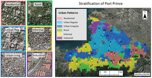
Figure 1. Map of the city of Port Prince divided into urban patterns. The different patterns are color-coded. Examples are shown to the left. The small numbered squares are the sample areas randomly chosen to conduct the present research.

There is no guarantee that any seismic building code was followed during reconstruction, as self-construction and spontaneous urban expansion were observed in the years following the event (Lallemant 2014). Furthermore, the seismic hazard in the region is still very high, according to a study by Symithe and Calais (2016). The authors affirm that the expected ground motion is double the values indicated in the hazard map for the current seismic code. The combination of high vulnerability and high hazard suggests that the seismic risk in Port Prince remains high.

To calculate the exposure and seismic vulnerability of the study area, we have relied on the following data sources.

Urban patterns and stratification

From our previous work (Wieland et al. 2016), we have taken the strata into which the city of Port Prince was divided after an object-based image analysis (OBIA). OBIA first segments the image into meaningful objects and then labels them using a classifier.

Each stratum represents an urban pattern with homogeneous street layout and similar building types. Figure 1 shows the stratification and the six urban patterns identified. Most of the city is dominated by the Urban patterns, both Regular and Irregular. These are areas with a high density where most buildings are simple in shape, usually rectangular. The difference between the Regular and Irregular patterns is that the Urban Irregular pattern is characterized by smaller buildings and a somewhat more chaotic, sometimes unpaved, road network. The city’s Residential districts are located in the east. The buildings in those districts are larger and of better quality; their shapes are more complex, and private gardens surround them with vegetation. The Informal stratum also covers a significant area within the city. These areas are depressed and full of small, poor-quality, overcrowded, self-built buildings. Building density is very high, and vegetation is scarce. The Rural areas on the city outskirts are large, open spaces with lots of greenery and detached buildings. Finally, a stratum dedicated to Industrial use was identified near the port. This stratum was excluded from the study because the vulnerability models available in the literature were developed mainly for residential buildings.

The subsequent task of detecting and classifying buildings was based on a stratified approach, using these urban patterns as strata, allowing for a better parameterization of the procedures of image and LiDAR analysis. The numbered boxes in each stratum represent the randomly chosen sample areas for this study.

Databases

After the 2010 earthquake, a significant amount of spatial information, from both public and private sources, was made available to the public over the Internet. In Table 2, we present the open data sources used in this study, either as input or as ground truth, as shown in Figure 3.

Table 2. Description of the data used in this study.

Data	Source	Reference System	Technical details
Orthophotos (RGB and SWIR)	Digital Imaging and Remote Sensing Laboratory (DIRS) at the Rochester Institute of Technology (RIT)	WGS-84	RGB images are in 16-bit Geotiff format with a ground sample distance (GSD) of 15 cm. The SWIR images are in the same format but with a GSD of 83 cm.
LiDAR point cloud	Collected by the RIT and Kucera International Inc. Downloaded from the OpenTopography website.	Horizontal: WGS-84 UTM18N. Vertical: EGM-96	The cloud was obtained using a Leica ALS60 sn/6133 sensor and has a density of 3.4 pts/m^2.
Cadastral building database (MTPTC DB)	Created by the Haitian Ministry of Public Works right after the 2010 earthquake (MTPTC 2010)	WGS-84	Contains 63,068 purged records for the study area with 28 fields including the coordinates (approximate location of a building) and other attributes relevant to the building’s typology and vulnerability (area, number of floors, and building materials). This database is used here to create predictive models for the building typologies.
Damage building database (CNIGS DB)	Collected in the frame of a collaborative project between the Centre National de l’Information Géo-Spatiale of Haiti (CNIGS), the World Bank, UNOSAT-UNITAR, and the European Commission’s Joint Research Center (JRC). (Corbane et al. 2011)	NAD1983 UTM18N	For each building, the database contains information on the building typology, number of floors, use, and the damage suffered in the earthquake. The study area for this study includes 2,728 buildings. This data is used here as ground truth when validating attributes and seismic damage.

All these data were loaded into a GIS that was used to manage the spatial information for the study. It should be noted that the MTPTC DB does not include all the buildings in the study area and that the locations are not precise (Figure 3) because they were taken using an autonomous, handheld GPS unit. In contrast, in the CNIGS DB, the location of each building is exact (Figure 3).

Building types

Torres et al. (2016) classified the buildings in Port Prince into six main categories (Model Building Types, MBT): four (4) with reinforced structures, either concrete or masonry; one (1) made of unreinforced masonry; and one (1) made of timber. All the buildings in the MTPTC DB were classified into these six MBTs, and it was observed that most of the buildings belonged to one of two typologies: buildings with a reinforced concrete structure and concrete block infill walls (75% of the total number of buildings) and buildings made of unreinforced masonry (17%).

Given this distribution, for the present study, we decided to group the rest of the buildings with these two predominant MBTs: all buildings with a reinforced structure were grouped with the first type, called RC. The reinforced structure can include either concrete or masonry, while the infills are made of non-reinforced concrete blocks. The quality of this type of building varies widely, as can be seen by comparing photographs A and B in Figure 2, which affects its vulnerability. According to our knowledge, the larger and taller this type of building is in Port Prince, the more resistant it will be (photo A). Therefore, one possible way to further subdivide this category could be by combining certain values of area and height. This is the predominant building typology in the city and the rest of the country and may be found in practically any downtown or suburban area.

Figure 2. Pictures of the different Model Building Types (MBT) identified in Port Prince.

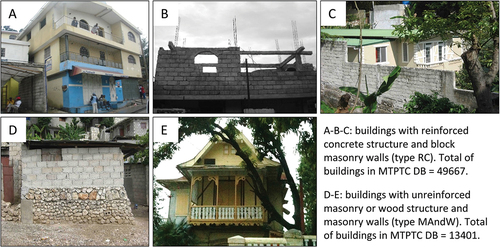
Wooden buildings and the unreinforced masonry building group were combined into a single category that we named MAndW (photographs D and E in Figure 2). Photograph D shows a typical unreinforced masonry dwelling in the city. These can be made of rock and/or blocks, with lightweight roofs made of wood and metal sheets. Photograph E represents a wooden construction typical of the French colonial period. This type of housing is actually very rare, counting only 699 buildings in the MTPTC DB (making 5% of the buildings classified as MAndW). In order to avoid unbalanced datasets in the subsequent machine learning steps, we did not separate the colonial buildings as one independent class.

Though simple, this grouping of categories is consistent with the local building stock and with previous studies, such as the work of Hancilar, Taucer, and Corbane (2013), who developed fragility curves for two similar typologies in Port Prince: reinforced concrete and wood.

Methodological framework

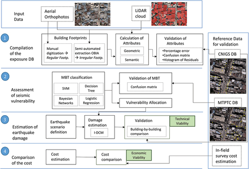
We present a description of the methodological procedure designed to (1) create an exposure database; (2) assign the buildings a vulnerability model; (3) estimate the damage an earthquake would produce; and (4) compare the cost of this study with the cost of studies conducted using traditional methods. Figure 3 shows a workflow diagram detailing each distinct phase and the techniques used in each phase.

Figure 3. Methodological framework followed in this study. Input data and ground truth data are in the blue boxes.

Compiling the exposure database

The database is a spatial database in which each record contains information about a building. This database is a valuable output in and of itself, as it offers a characterization of buildings that, if sufficiently comprehensive, could be used to assign vulnerability with respect to other types of natural hazards (floods, fires, tsunamis, etc.), thus meeting the needs of a multi-hazard approach.

This phase is, in turn, divided into two phases: generating building footprints and calculating attributes. Both outcomes must be validated.

Creating building footprints

As no official footprints were available, these had to be generated specifically for the study. Two different procedures were used to compare the outcomes: Object-Based Image Analysis (OBIA) and manual digitization. The polygons obtained using OBIA were designated as irregular footprints and the digitized polygons as regular footprints. RIT orthophotos were used in both cases, and LiDAR was also used as part of the OBIA analysis.

The regular footprints were digitized manually in ArcGIS, using the orthophotos as a reference, after first processing these to create mosaics. Mosaics were created to merge the various orthophotos that overlapped in each sample area, in order to get one single raster image, which is easier to manage and analyze. During the manual digitizing process, in addition to creating the geometry, a label was given to each building to indicate the roofing material, an important attribute for estimating seismic vulnerability.

The irregular footprints were generated by means of an OBIA analysis with two phases, namely segmentation and classification. For segmentation we used the Felzenszwalb and Huttenlocher (2004) powerful graph-based edge search algorithm. The algorithm generates regions of pixels with similar values, called segments, using the Euclidean distance to measure dissimilarity. The scale parameter (s) sets the differentiation threshold, as larger values generate larger segments. The merge parameter (m) controls minimum segment size. Parameterization is generally carried out through trial and error until the resulting segmentation outlines the contours of the objects of interest satisfactorily.

The resulting segments were then classified into the following categories: concrete roof, metal roof, pavement, shadow, and vegetation. The classifier used to label segments in this phase was Random Forest (Breiman 2001). This ensemble algorithm creates decision trees using a different subset of feature vector attributes each time. The final class assigned to a certain instance is the class with the most votes out of all the trees in the forest. The feature vector was composed by three types of attributes: spectral: minimum, maximum, mean, median, mode, variance, and kurtosis coefficient; textural: contrast, dissimilarity, homogeneity, and ASM; and geometric: area, perimeter, and Degree of Compactness (DC). The latter was calculated as defined by Cerri (2018), DC = Area·4·π/perimeter². Its value varies between 0 and 1. To tune the random forest, the user sets parameter k, which is the maximum number of attributes to be selected. Two other key attributes that must be adjusted are the tree depth (f) and the minimum number of samples (mS) left in a node when the condition established for the node is met. All these parameters were tested through cross-validation with ten iterations (10%) to determine which combination of parameters provided the highest accuracy.

For validation, we compared the number of building footprints created through OBIA with the number of digitized footprints, using the latter as a reference to analyze the difference between the two.

Calculating building attributes

Various taxonomies propose a series of building attributes that affect the way buildings behave when subjected to seismic shocks and should therefore be included in an exposure database (e.g. FEMA 1992 Risk-UE LM2 [Milutinovic and Trendafiloski 2003]). Consistent with the Sendai Framework, the most recent of these taxonomies apply a multi-hazard approach, given the clear distinction between the concepts of exposure (common to all risks) and vulnerability (which is particular to each risk). The present study used the GED4ALL taxonomy (Silva et al. 2018) as a reference, but with certain adaptations presented in Table 3. The study aims to adopt the Sendai Framework’s recommendation of making multi-hazard systems more widely available.

Table 3. List of building attributes calculated to create the exposure database (adapted from GED4ALL taxonomy). Name, definition, calculation method and possible values are provided.

Building Attribute	Calculation method
Ground Area	Directly computed in the GIS
Centroid location (X,Y)	Directly computed in the GIS
Direction	Azimuth of the minimal enclosing rectangle of each footprint, considering the direction of the longest side (length). Values ranging from 0º to 180º.
Shape of the Building Plan	Given by two indicators: Elongation: width/length. Ranges between 0 and 1. Very elongated footprints yield values close to zero. More compact, square shapes present values close to 1. Degree of compactness: following Cerri (2018) as explained before.
Building Position within the Block	Considers whether a building is detached or is adjacent to one, two or three buildings. A spatial query in the GIS is used to find adjacent buildings with the search distance set to 4% the building height.
Height	The height is computed as the median of all the nDSM cell values inside a footprint. From the height (in meters), the number of stories is derived by dividing it by the typical floor height of each stratum.
Roof	Given by two indicators: Roof Shape, to distinguish between flat and pitched. The roof slope is computed as the average of the slope of all the triangles of the TIN created inside each footprint (Yolanda et al. 2019). The slopes of the triangles are weighted using their area in order to minimize the influence of small triangles (q. 1). $Pt{e}_t=\sum i=1nPt{e}_i\cdot A_i\sum i=1n{A}_i$ Eq. 1. Roof slope Where Ptet is the roof slope computed with the n triangles of its TIN. Ptei and Ai are the slope and area of each triangle, i. Roof Covering denotes the roofing material. It is a semantic attribute with two values: Concrete roof and metal roof. These values have already been obtained in the previous phase of footprint creation.

The attributes calculated in this study are listed in Table 3. It is important to comment about the absence of the year of construction. We conducted a change control analysis using Landsat images from 1973, 1989, 1999, and 2010. The outcome indicated that most of the buildings in Port Prince were built before or during the 1970s and 1980s. The informal settlements in the southern part of the city were built in the 1990s. Although the analysis yielded a valuable estimate of urban expansion, it turned out that the year of construction for every single building was merely approximate. Given its low discriminant power, this attribute did not appear to be very useful in helping predictive models distinguish between different building types in the city under study.

The age of the building might offer information about its condition and state of repair. For the purpose of characterizing vulnerability, the date of construction becomes particularly relevant in cities that have historically adopted seismic-resistant building codes, which is not the case in Port Prince.

Given the foregoing, we decided not to consider this attribute for MBT classification.

The building attributes listed in Table 3 were computed and validated to measure their accuracy level and then used to assign each building a seismic vulnerability model. Geometric attributes (i.e. location, position in the block…) were not validated because they were calculated directly in the GIS and are considered correct. The area, the roofing material for buildings with irregular footprints, and the height of both sets of footprints were validated.

The ground area was verified using a comparison coefficient obtained by dividing the total area covered by irregular footprints (considered an estimate) by the total area occupied by regular footprints (considered ground truth). This was calculated for each stratum and the total number of footprints.

The number of floors obtained using the LiDAR nDSM for both sets of footprints was validated using the histogram of the residuals, with the CNIGS DB serving as ground truth.

The roofing material for buildings with irregular footprints was validated using a confusion matrix created with a testing dataset that compares the label assigned to each roof by the classifier in the OBIA process with a label created through photo interpretation. Several accuracy metrics were obtained based on the matrix (Fawcett 2006). Of all the metrics, the overall accuracy, F1-Score, and Cohen’s kappa coefficient of agreement are presented here. The overall or global accuracy was calculated as the quotient between the total number of correctly classified samples and the total number of samples. The F1-Score is the harmonic mean of accuracy and recall (the ratio of the number of correctly classified samples in a class to the total number of samples in that category). This comprehensive measure of accuracy balances the cost of false positive and false negative errors. Its use is indicated when sample datasets are unbalanced (when the various categories do not include the same number of samples). The values for both measures are expressed as percentages, with higher percentages indicating better classification results. Finally, the kappa coefficient compares observed and expected accuracy, the latter being a measure of how much the results obtained by a classifier differ from the results that would have been obtained by randomly classifying the sample. This indicator is complementary to the metrics mentioned above. The present study applied the scale proposed by Landis and Koch (1977) to interpret this indicator: κ < 0.00, poor agreement; 0.00 ≤ κ ≤ 0.20, slight agreement; 0.21 ≤ κ ≤ 0.40, fair agreement; 0.41 ≤ κ ≤ 0.60, moderate agreement; 0.61 ≤ κ ≤ 0.80, high agreement; 0.81 ≤ κ ≤ 1.00, near-perfect agreement.

To ensure a more robust validation of this attribute, the roofing material for all buildings with irregular footprints was compared with the roofing material for those with regular footprints, which is considered ground truth to this end.

Assessing seismic vulnerability

This phase consists of two steps: first, the buildings in the sample areas were classified into the two MBTs identified previously and then assigned a vulnerability model.

Classifying buildings into MBTs

The buildings in the sample areas were classified into the two building typologies described above: RC and MAndW. To this end, predictive models were created using instances from the MTPTC DB that lie outside the sample areas but within each stratum. Prediction models were created based on the following attributes: area, number of floors, roofing material, and centroid coordinates. Since these attributes are found in both the MTPTC DB and the exposure DB generated in this study, the typology classification models may be applied to the data generated in the sample areas. Before training the models, the attributes were ranked by discriminant power, from highest to lowest, using the ReliefF algorithm in WEKA. ReliefF (Kononenko 1994) establishes a ranking of attributes according to their capacity to discriminate between neighboring samples in different categories.

The models were trained using decision trees, SVM, the naïve Bayesian classifier, and logistic regression. Since the number of attributes was very limited, we were able to use these last two classifiers, which are simpler. In addition to obtaining a classification model, one of the objectives was to determine which attributes have the most significant impact when identifying a building typology.

The decision trees were created using the C4.5 algorithm proposed by Quinlan (1993). A decision tree is a hierarchical representation of conditions defined based on the attribute values for the training samples. These conditions are used to separate the samples into categories. The tree depth is controlled through parameter f.

SVM (Support Vector Machines; Vapnik 2000) is a non-parametric statistical classifier that uses a kernel to represent samples in a higher dimensional space where the samples can be separated linearly. The SVM can then draw the hyperplane separating these samples with the goal of making the margin between the hyperplane and the samples as big as possible. Parameter C controls the balance between the size of the margin and the classification errors for samples closer to the hyperplane (the support vectors). The present study tested two kernels to create the models using SVM. One is the Radial Basis Function (RBF) kernel, which requires adjusting the width, gamma, (γ). And the other is the Pearson VII Universal Kernel (PUK, Ustun, Melssen, and Buydens 2006), which requires two parameters: sigma (σ) for the half-width of the Pearson VII function; and omega (ω) for the tailing factor.

The naïve Bayesian classifier is a statistical model that expresses the conditional probability of a class based on the attribute values of the (previously discretized) training samples. The probability that a given instance will be classified as a certain class is calculated using Bayes’ Theorem. Finally, binary logistic regression is used to calculate the likelihood that a given instance belongs to one class versus another as a linear function of the attribute values for the training samples. These last two classifiers are easier to implement because they need not be parameterized.

The models were trained through cross-validation with ten iterations in WEKA, and the final parameters were adjusted using a Python code (Arredondo 2019) based on the well-known Scikit-Learn open source machine learning library. The models were validated by means of a confusion matrix and then calculating accuracy metrics.

Allocating a vulnerability model to each MBT

Once all the buildings had been classified as one of these two building typologies, they were then assigned a vulnerability model as described in Molina et al. (2014). A vulnerability model is defined by two curves [capacity spectrum-fragility function], referred to as damage functions, that represent the behavior of a given type of building in the event of an earthquake. Molina et al. (2014) initially allocated a vulnerability model taken from the literature to the six MBT previously described in the Building Types section. Then, they calibrated the damage functions using the damage data stored in the MTPTC DB to create a new vulnerability model for each MBT that is specific for the Haitian building types. Out of the six vulnerability models that the authors created, two have been allocated to the MBT considered in the present study: RC-CB is assigned to the RC typology; and CM-UM is assigned to the MAndW building type. RC-CB and CM-UM are comparable to the vulnerability models RC1-I and M6-Medium code of Lagomarsino and Giovinazzi (2006), respectively, thus Molina et al chose them as initial curves in the calibration process. The final parameters of the pair of damage functions, after calibration, can be found in Molina et al. (2014). We do not reproduce them here for the sake of space. Each typology was subdivided by height range, based on the description provided by the authors, into low-rise (1–3 floors) and mid-rise (4–6 floors).

Estimating earthquake damage: technical viability assessment

In this section, we will try to evaluate to what extent the errors made in classifying building typologies can affect damage results. Damage was estimated using SELENA (Molina, Lang, and Lindholm 2010). We applied the attenuation models proposed by Boore et al. (2014) and Chiou and Youngs (2014) and combined them to form a logic tree with a weight distribution of 60%-40%, respectively, in keeping with the criteria established in previous studies (Molina et al. 2014; Torres et al. 2016). The value of V_s³⁰, which characterizes the soil type, was taken from Cox et al. (2011). All this data was used to calculate the demand spectrum for each geo-unit of the study.

The Improved-Displacement Coefficient Method (I-DCM, FEMA 2005) was applied in SELENA to estimate the damage that the simulated earthquake would cause to the buildings. I-DCM is an inelastic, non-linear method of analysis that can be used to calculate the maximum displacement a building might be subjected to in a seismic shaking event. On the other hand, the fragility function describes the damage distribution corresponding to this maximum displacement within five degrees that have direct correspondence with those from the EMS-98 scale (Grünthal 1998): Null (D0 - no damage); slight (D1 - Slight); moderate (D2 – Moderate); extensive (D3 – Heavy); and complete (D4 – very Heavy and D5 – Destruction).

Cost comparison: economic viability assessment

This last phase studies the economic feasibility of creating exposure and vulnerability databases using remotely sensed data. The cost is considered economically viable if it is lower than the cost of conducting an in-field survey to collect information on buildings to generate the same product. To address this issue, the cost of conducting a remote sensing study to classify 1,000 buildings was compared to the cost of conducting a field campaign for the same purpose in both, a city in a developed country and a city in a developing country (like the one in this study). This furthers the Sendai Framework’s objective of improving international cooperation with developing countries to address seismic risk.

The execution of the present study and other similar studies carried out by the authors in different scenarios was taken as a reference to estimate the cost of the remote sensing work. Twelve national and international experts with accredited experience in on-site building inspection were asked to collaborate on a nonprofit basis to assess the cost of a field survey. These experts collaborated by filling out a form prepared specifically for this research study or by making comments and suggestions based on their experience in the field. The form can be downloaded from Mendeley Data with the name “Template – Building In-Field Survey.” For each scenario, the experts provided data on the resources (human and material), time, and costs involved in evaluating 1,000 buildings in situ. The form they filled out distinguishes between tasks carried out before the field visit, the visit itself (including travel), and post-processing work.

Results and analysis

Implementing and validating the exposure and vulnerability database

This section corresponds to phases 1 and 2 of the general methodological framework (Figure 3).

Exposure database compilation

Building footprints

First, the building footprints were generated by manually digitizing each of the 24 sample areas. To do so, orthophoto mosaics were created with the 4 bands provided by RIT (RGB+SWIR). A total of 6,414 buildings were digitized, which on average took 5 seconds per building for Urban areas and Informal settlements (whose buildings have a simple square or rectangular shape); and 10 seconds for Residential and Rural areas (whose buildings tend to have more complex shapes). It is important to mention that within this time, both the building footprint is drawn and the value of the roof type attribute (concrete or metal) is written in the database. The latter is done automatically by the software (ArcGIS) provided that a template for the corresponding roof covering is selected before drawing. This allows for speeding up the process of digitization and labeling. A total of 2,146 buildings have concrete roofs, while 4,268 (almost twice as many) have metal roofs.

On the other hand, OBIA was used to create the irregular footprints. This was done by preparing nine (9) bands: four (4) with the orthophotos (RGB+SWIR), three (3) with the spectral differences (R-G, R-B, G-B), and 2 derived from LiDAR – using the intensity of each point and the normalized Digital Surface Model (nDMS) to calculate the height above ground level for each point. The nDSM was created after classifying LiDAR points using the MDTopX TOD algorithm (Yolanda et al. 2019). To carry out the OBIA process, a Python code was created using the following libraries: Pandas, for manipulating tabular data; Rasterio and Scikit-image, for managing images; Scikit-learn, for machine learning; Matplotlib and Seaborn, for visualization. The code is published on GitHub (Arredondo 2019).

For segmentation, Felzenszwalb and Huttenlocher (2004) algorithm was used with the three (3) visible bands (RGB) and LiDAR heights. The best results were obtained by applying the following parameters of scale (s) and merge (m), by stratum: Residential (s = 100; m = 1000), Urban Regular (s = 70; m = 800), Urban Irregular (s = 60; m = 600), Rural (s = 50; m = 600), Informal (s = 50; m = 600). Obviously, in keeping with reality, the objects of interest (buildings) are larger in Residential areas, medium-sized in Urban areas, and smaller in Rural areas and Informal settlements.

To classify the resulting segments, two datasets were randomly created with the following number of samples for training (tr) and testing (te): concrete roof (tr = 221, te = 69), metal roof (tr = 290, te = 56), pavement (tr = 153, te = 45), shade (tr = 116, te = 26) and vegetation (tr = 116, te = 29). A 102-dimensional feature vector was computed for all the samples and used in a random forest of 100 trees, which was trained by varying the parameter values: k = {√ (n), log2 (n)}, being n the dimension of the feature vector; f = {none, 5, 3, 1} (none means that each tree is built with the number of nodes needed to ensure all the leaves are as pure as possible); mS = {1, 5, 20, 100}. After cross-validation at 10%, the final values that yielded the highest accuracy were: k = √(n); f = none; mS = 1.

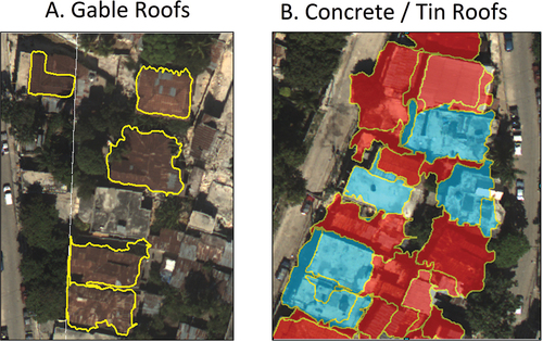
Various combinations of bands were also tested to obtain the highest possible accuracy. The LiDAR-derived height band proved decisive in the segmentation process as it enabled us to obtain a correct footprint on most of the gable roofs (Figure 4a), which are often over-segmented. Regarding classification, the data from LiDAR played a key role in helping to distinguish concrete roofs from metal roofs (Figure 4b). On the other hand, SWIR did not seem to offer any significant improvements. Material validation is covered in the next section.

Figure 4. Examples of roofs extracted with OBIA. (A) Gable roofs. (B) Two types of roof materials: Concrete roofs, in blue; metal (tin) roofs, in red.

Based on this OBIA analysis, we were finally able to determine which segments belonged to roofs: a total of 6,985 polygons. Moreover, this process enabled us to identify the roofing material.

The roof segments were validated using the digitized roofs in 21 of the 24 sample areas as a reference. The areas with ID = {10, 17, 22} (Figure 1) were discarded from the validation and the rest of the study because most of the buildings in these areas were in ruins due to the earthquake. The estimated total number of buildings (based on OBIA) and the actual number of (manually digitized) buildings were 6,293 and 5,068, respectively. The comparison coefficient between the two is 1.25, indicating that there are 25% more segments than building roofs. This discrepancy was to be expected given the complexity of many of the roofs, particularly in Residential areas, which are often over-segmented.

In the Informal pattern, the comparison coefficient is generally around 1, indicating a proper segmentation of the roofs. In this stratum, the buildings are small and simple, making it easier to identify them using OBIA. No single predominant type of roof exists in the Urban Regular, Urban Irregular, and Rural patterns. This variability is reflected in the comparison coefficients, which range from 0.94 to 2.52 in those strata.

Building attributes

All attributes were calculated for both regular and irregular footprints. Figure 5 shows the values for a sample area in the Residential stratum. The attribute table corresponds to the building highlighted in deep red. As we can see, the two sets of footprints in this example do not present any significant differences in their attribute values.

Figure 5. Attributes stored in the exposure database of the buildings present in one residential sample for both, regular (A) and irregular (B) footprints. The windows show the attributes of the buildings in deep red, as an example.

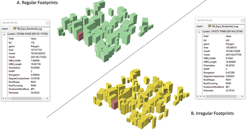
The estimated total built-up area (based on OBIA data) is 33.1 ha, and the actual area (estimated through manual digitization) is 29.6 ha. The comparison coefficient between the two is 1.12, i.e. the percentage error in calculating the built-up area is 12%. This implies that the area of a 100-m² building would be estimated at 112 m², which has little impact on how its building typology would be classified. The only stratum for which the area is underestimated is the Residential stratum, but the comparison coefficients are very close to 1. This pattern had the highest number of segments per footprint, which is to be expected, since the more over-segmented a roof is, the more detail we will obtain about its shape and size. In the Informal and Urban Irregular patterns, it seems we managed to strike a balance between the number of segments and the built-up area, as the comparison coefficient for most of these areas is around 1. In the Urban Regular pattern, we observe the same variability as with the number of footprints, with area comparison coefficients ranging from 1.03 to 1.23. The area for buildings in Rural areas was overestimated by more than 20%.

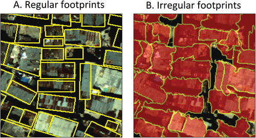
The spatial intersection between the segmented and digitized footprints was also calculated. The total area of the intersection is 23.74 ha, which results in a total detection rate of 80% (intersection area compared to the actual area). The primary discrepancy between the area estimated in the OBIA analysis (irregular footprints) and the area calculated based on digitization (regular footprints) is that the former does not create gaps between buildings while the latter does. A typical example is the sample area ID = 3 (comparison coef. = 1.24), shown in Figure 6.

Figure 6. Illustration of the gap between buildings as the main source of discrepancy in the built-up area estimation. Examples are provided for a regular (A) and an irregular (B) footprint.

To validate the roofing material obtained through OBIA, a confusion matrix was calculated and used to derive the accuracy and F1-Score metrics (Table 4). As we can see, the quality measures are very high; most are above 90%. This part of the study focused on identifying the roofing material, which had an F1-Score of 99% for concrete and 95% for metal. The LiDAR-derived height band was key in distinguishing concrete roofs from pavement (both have a similar spectral response in the imagery) to the extent that none of the instances of these classes were misclassified.

Table 4. Confusion matrix of the image classification process with OBIA. Accuracy measures are given for the five classes identified. Concrete roof and metal roof are of particular interest for the present study.

	Predictions					Accuracy measures
	Concrete Roof	Pavement	Shadow	Metal Roof	Vegetation	Precision	F1-Sc
Concrete Roof	68	0	0	1	0	99%	99%
Pavement	0	45	0	0	0	98%	99%
Shadow	0	0	24	1	1	86%	89%
Metal Roof	1	1	0	54	0	93%	95%
Vegetation	0	0	4	2	23	96%	87%
Average:						95%	95%

On the other hand, the LiDAR-derived intensity data enabled us to distinguish the materials of the two types of roofs (concrete and tin), which, in many cases, were misclassified. For the most part, shadows and vegetation were mistaken for each other, but these classes are not of interest for this study. Overall, the results of this classification are highly satisfactory, with a 95% weighted average for the three metrics and a near-perfect Cohen’s kappa coefficient of 0.94.

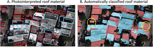
The roof type obtained through OBIA was compared with the information collected during the digitizing process. Of the 6,985 segments classified as buildings through OBIA, it was found that 393 (only 5.6%) did not intersect with the digitized footprints, either because they were on the edges of the study areas or because the segments belonged to other types of constructions (courtyards, walls, ruins, etc.). Of the remaining 6,592 segments, 5,479 were correctly classified as concrete and metal, representing an 83% overall accuracy. Of the segments classified as belonging to metal roofs, 13% were actually concrete roofs; and 4% of segments classified as concrete roofs were actually metal roofs. Figure 7 shows an example of this comparison.

Figure 7. Comparison of roof material obtained by photo interpretation (A) and OBIA (B). Concrete roofs are in blue; metal roofs are in red. Yellow circles mark examples of classification errors.

Finally, the number of floors was verified using the CNIGS DB. This verification was carried out for both regular (digitized) and irregular (segmented) footprints. Of the 6,492 buildings in the CNIGS DB, only 356 fall within the sample areas for this study; of those, 295 intersect with regular footprints, and 289 intersect with irregular footprints. The rest are collapsed buildings that Corbane et al. (2011) documented to calculate their fragility curves, but they were not taken into account in the present study. For the buildings that match, we calculated the residual for the number of floors (the difference between the estimated number of floors and the number of floors observed in the CNIGS DB) and created a histogram. Most of the residuals were equal to zero. For regular footprints, the overall accuracy (OA) obtained was 79%; for irregular footprints, the OA was 72%. Of the remaining residuals, most were 1-floor (18% for regular footprints and 26% for irregular footprints). The most significant errors in estimating the number of floors were 2-floor excesses and 3-floor deficits, but these errors account for less than 3% of the total number of buildings verified. Vulnerability models group buildings in ranges of 2 or more stories, so an error of 1 or 2 stories may not be very significant for this study.

Seismic vulnerability assessment

Building type classification

The techniques described in the methodological framework sections were used to create predictive models to classify the buildings into MBT. The training and testing datasets (Table 5) are balanced and were generated using stratified random sampling.

Table 5. Number of samples in the training and testing datasets for MBT classification.

	Training		Testing
	RC	M&W	RC	M&W	Total
RESIDENTIAL	240	240	60	60	600
URBAN REG.	1600	1600	400	400	4000
URBAN IRREG.	3200	3200	800	800	8000
RURAL	120	120	30	30	300
INFORMAL	3200	3200	800	800	8000

Predictive model training using data out of the sample areas

After ranking the attributes in WEKA using ReliefF, the order obtained for most strata was: roof type, number of floors, area, centroid X-coordinate, and centroid Y-coordinate. The area came in last place in Rural and Urban Regular patterns, indicating that the building ground floor in these strata varies greatly; therefore, the area turn out not to be a decisive attribute for classifying building typologies in those strata.

The models were then trained. The parameters varied within the following range of values: f = {2, 3, 5}; C = $\gamma$ =$\omega$ = {0.01, 0.1, 1, 10, 100}. Table 6 summarizes how each model performed, indicating the overall accuracy attained during the training phase and the best parameters. It may be observed that the best models were the SVM models, especially those with a PUK kernel, which reached accuracies between 88% and 100%. All the models were more accurate when applied to Urban and Residential patterns, with values above 79%. It seems that buildings in those districts were built using more standardized construction methods than those in Rural and Informal patterns, where the overall accuracy drops to 70% (even though SVM with PUK results in very high accuracy in these strata). It’s worth noting how well the naïve Bayes classifier performed. This was the simplest of all the models implemented, yet it obtained accuracy measures comparable to the rest.

Table 6. Parameters and performance of the predictive models created to classify buildings into MBT. OA stands for Overall Accuracy; Param. stands for parameters tuned for each classifier; SVM (PUK) stands for support vector machine with Pearson VII Universal Kernel; SVM (RBF) stands for support vector machine with radial basis function kernel.

	Decision tree		SVM (PUK)		SVM (RBF)		Logistic Regress.	Naïve Bayes
Stratum	OA	Param.	OA	Param.	OA	Param.	OA	OA
Residential	82%	f = 3	88%	C = 1; σ = 1; ω = 1	86%	C = 1; γ = 1	83%	80%
Urban reg.	82%	f = 3	91%	C = 1; σ = 0.01; ω = 0.1	81%	C = 0.01; γ = 0.1	81%	81%
Urban irreg.	80%	f = 3	100%	C = 10; σ = 10; ω = 0.01	84%	C = 1; γ = 10	79%	79%
Rural	78%	f = 3	98%	C = 10; σ = 1; ω = 0.1	83%	C = 1; γ = 1	73%	73%
Informal	70%	f = 3	100%	C = 10; σ = 0.01; ω = 0.1	79%	C = 1; γ = 10	70%	70%

It is important to understand what attributes have the most significant impact when identifying MBTs. Every tree uses the roof as the first attribute and then works with the coordinates. The only exception is the Residential stratum, where the trees move on to work with the area. The number of floors was used only in the Informal and Rural strata. The area only appears in the Residential and Regular Urban strata. This favors irregular footprints, which tend to have less realistic areas. With logistic regression, variables such as roof type, number of floors, and area (in that order) were used to generate the equation in every stratum. This is in line with the attribute ranking provided by ReliefF.

Validating and selecting the best predictive model

All the models created in the previous step were validated using the testing (unseen) samples in Table 5 to check their generalization capacity. The model ranking for each stratum is presented in Table 7. The best model for all strata is the model calculated using SVM and a PUK kernel, followed, in most cases, by SVM with an RBF kernel. The decision tree and logistic regression obtained similar performance rates, as did the naïve Bayes classifier. As mentioned in the training phase, it is worthy to remark the capacity of the naïve Bayes also in the testing phase. Despite its simplicity, it obtained accuracies comparable to other more sophisticated techniques, such as SVM. SVMs prove their potential when working with databases containing noise, as in the Informal stratum, where SVMs maintained overall accuracies and F1-Scores above 70% while the other models did not.

Table 7. Predictive models created for each stratum. Models are ranked by performance. Overall Acc. stands for Overall Accuracy; kappa is the Cohen’s kappa coefficient of agreement; SVM (PUK) stands for Support Vector Machine with Pearson VII Universal Kernel; SVM (RBF) stands for support vector machine with radial basis function kernel; logistic reg. stands for logistic regression.

Machine Learning Algorithm	Overall Acc.	F1-Score	kappa
	RESIDENTIAL
SVM (PUK)	88%	87%	0.75
SVM (RBF)	88%	87%	0.75
Logistic Reg.	87%	87%	0.73
Decision Tree	87%	86%	0.73
Naïve Bayes	87%	86%	0.73
	URBAN REGULAR
SVM (PUK)	82%	81%	0.64
Decision Tree	82%	81%	0.64
SVM (RBF)	81%	81%	0.63
Logistic Reg.	82%	81%	0.63
Naïve Bayes	81%	80%	0.62
	URBAN IRREGULAR
SVM (PUK)	81%	81%	0.62
SVM (RBF)	80%	80%	0.60
Logistic Reg.	80%	79%	0.60
Naïve Bayes	80%	79%	0.60
Decision Tree	80%	79%	0.59
	RURAL
SVM (PUK)	78%	78%	0.57
Decision Tree	75%	73%	0.50
SVM (RBF)	73%	73%	0.47
Logistic Reg.	70%	68%	0.40
Naïve Bayes	70%	68%	0.40
	INFORMAL
SVM (PUK)	74%	74%	0.49
SVM (RBF)	73%	73%	0.47
Decision Tree	70%	68%	0.40
Logistic Reg.	70%	67%	0.39
Naïve Bayes	70%	67%	0.39

A general reduction in quality may be observed in the Rural and Informal patterns, as was the case during the training phase. As many of the buildings in these areas do not comply with standards, the data tends to be much more random, making it harder to classify. The best accuracies obtained for these patterns were as high as 78% (equal to F1-Score) for Rural areas and 74% for Informal settlements. For Urban areas, values were as high as 81% for irregular footprints and 82% for regular footprints. Finally, the most accurate classification was for Residential buildings, with accuracies of 88% and an F1-Score of 87%. The kappa values indicate moderate agreement between the model prediction and reality for the Informal and Rural strata while show high agreement for the Residential and the two Urban patterns.

Given the performance demonstrated by the various models, we chose to use the model created using SVM with a PUK kernel to classify the buildings in the sample areas.

Table 8 shows the confusion matrices for this model. We can see that the MAndW class has a high rate of false positives worth analyzing. It was found that the most relevant attribute for determining the classification of concrete or masonry buildings was the roof type. Reinforced concrete roofs are found on buildings whose structures are also made of reinforced concrete. However, roofs made of metal sheets can be seen on both small wooden dwellings and/or masonry buildings (Figure 2 (D)), as well as on buildings with a reinforced structure (Figure 2 (C)). This makes it difficult to distinguish between the two typologies when the roof is made of metal. One explanation for the percentage of false-positive errors with the MAndW class in all models is that most buildings in this city have metal roofs. The models tend to classify constructions with metal roofs as MAndW buildings.

Table 8. Confusion matrices of the best predictive model for MBT classification: support vector machine with Pearson VII universal kernel. matrices are given per stratum.

	Prediction Residential		Prediction Urban Reg.		Prediction Urban Irreg.		Prediction Rural		Prediction Informal
	RC	WAndW	RC	WAndW	RC	WAndW	RC	WAndW	RC	WAndW
RC	47	13	259	141	535	265	24	6	519	281
WAndW	2	58	4	396	40	760	7	23	131	669

Although ideally, there should be minimal errors, the fact is that, in this case, this distribution of errors is favorable. The MAndW false positive error indicates that a concrete building is classified as masonry, i.e. the classifier says that it is more vulnerable to earthquakes. This is likely to result in overestimating damage, which would be a more conservative scenario and justify building inspection policies and a more in-depth study of seismic risk for the city.

Classifying buildings inside the sample areas into MBT

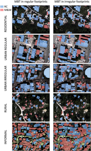
The SVM (PUK) model was applied to the exposure database of the buildings in the sample areas, and all buildings were classified into the two MBTs. Both regular and irregular footprints were classified. Figure 8 presents a sample area with the classification for each stratum. As observed, for each group of footprints, the Rural and Informal strata contain more discrepancies. These strata are the hardest to classify because they tend not to follow construction standards.

Figure 8. Results of building classification in MBT. Left column: Examples of regular footprints in each urban pattern. Right column: Corresponding examples for irregular footprints.

Vulnerability model allocation

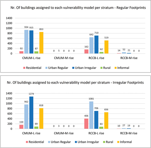
Each building was assigned a vulnerability model according to its MBT, as established in the section on methodology: RC-CB was assigned to the reinforced concrete (RC) typology and CM-UM to masonry and wood (MAndW) constructions. Figure 9 shows the distribution of vulnerability for both regular and irregular footprints in all the patterns analyzed. The vast majority of buildings are low-rise (less than three stories).

Figure 9. Distribution of vulnerability in the different urban patterns (also named strata). Labels over the columns indicate the number of buildings assigned to each vulnerability model per stratum (color-coded).

Estimating the damage scenarios

This section describes how the damage was estimated after simulating a probable earthquake in the area. With SELENA we simulated a Mw 7.0 earthquake on the Enriquillo fault segment analyzed by Symithe and Calais (2016), with epicenter located about 20 km from Port Prince. The source parameters used were as follows: epicenter coordinates in WGS84 (lat = 18.5042º; lon = −72.1184º); depth = 5 km; orientation = 270º; dip = 90º; mechanism = strike-slip.

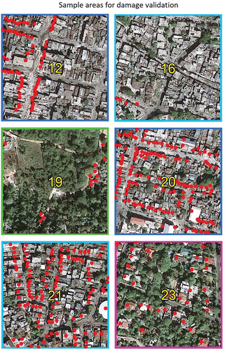
The estimation was carried out by preparing three vulnerability databases to compare the damage results obtained with each of them: (1) the Reference DB was the CNIGS DB; (2) the RegFootp DB, composed of buildings whose footprints were digitized in this study and found to match the footprints in the Reference DB (295 buildings); (3) the IrregFootp DB, composed of buildings whose footprints were obtained using OBIA in this study and found to match the footprints in the Reference DB (289 buildings). The buildings of these three databases overlapped in six sample areas with FID = {12, 16, 19, 20, 21, 23} (Figure 10). Hence, they are chosen for this phase of damage estimation.

Figure 10. Sample areas in which the validation of the damage assessment was conducted. Red points are the buildings whose damage estimation has been validated. The frames of the samples are color-coded according to the urban pattern also used in Figure 1.

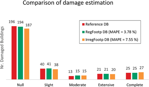
The damage results obtained using the three vulnerability DBs are indicated in Figure 11. The estimated number of damaged buildings are practically the same for all three datasets, with a MAPE of 3.78% for buildings with regular footprints and 7.55% for those with irregular footprints. The damage distributions indicate that most buildings in the six sample areas (66%) would not experience damage from the earthquake simulated in this study. Of the damaged buildings, approximately half (14% of the total) would sustain light damage. In comparison, the other half (16% of the total) would suffer severe damage or collapse, and only a minority (4%) would present moderate damage.

Figure 11. Damage distribution. Labels over the columns indicate the number of buildings reaching each damage grade. The results obtained with each vulnerability database are color-coded.

Given these low error rates, it is reasonable to conclude that the two vulnerability estimates made in this study would be valid for assessing seismic risk in a city.

Evaluating the cost

The cost of generating the database for 1,000 buildings using remote sensing was estimated based on the authors’ experience. An effort was made to be as realistic as possible. Thus, this estimate does not include tests or experiments, which are more typical of a research-based approach. The list of tasks is presented in Table 9. It should be noted that tasks 3.1 and 3.3 are mutually exclusive. Therefore, depending on the city in question, it will be necessary to choose one or the other. The times were estimated based on a work team of two people: a data scientist or engineer and an experienced collaborator (assistant). Ideally, the team should have a certain level of expertise in the study area and local construction methods to make the best possible decisions throughout the process. Failing this, we recommend meeting with a local civil engineering or architecture expert for two days before and during the study. We estimate it would take a maximum of ten days to generate the exposure and vulnerability database for 1,000 buildings using remote sensing. The workday contemplated is a standard 8-hour workday. It is important to note that the estimated time commitment was padded to account for any potential difficulties. This is evident upon comparison with authors such as Wenhua et al. (2017) who have provided this information from similar studies and reported a 10-day work period to analyze an area twenty times the size (456 km²).

Table 9. List of tasks and time estimation to create an exposure and vulnerability database for 1000 buildings using remote sensing and machine learning techniques.

Task	Time (working days)
(1) Data gathering, pre-processing, and integration in a GIS	2
(2) Stratification of the city Sampling process OBIA: training and testing	1
(3) Generación de la base de datos de exposición Manual digitization and photo interpretation (footprints and roof material) [exclusive with 3.3] LiDAR classification OBIA: sampling, training, and testing (footprints and roof material) Computation of attributes Related to LiDAR (height, number of stories, roof slope) Related to the footprint geometry	1/2 2 1 1
(4) Building type classification Sampling process Predictive modeling: training and testing	1
(5) Vulnerability allocation	1

Regarding material resources, the estimate contemplates using two computers plus office equipment. Obtaining the data would probably not entail any additional cost because it would be freely available (as it was for the present study). Should this prove impossible, data should be purchased or collected. In such a case, according to our experience and after consultation with various experts from remote sensing companies, an estimated price for the approximate 2 km² of orthophotos and LiDAR would be of the order of € 1,000.

We have estimated the costs associated with these resources. Human resources would amount to €4,500, including the following allocations: data scientist: €250/day; assistant: €150/day; local expert: €250/day (the latter would work only two days for meetings). The estimated cost of the material resources is about €3,000 (including the total cost, without accounting for proportional amortization), which comes to €7,500. A 30% margin was added to account for potential contingencies, bringing the total cost estimate to €9,750. In the authors’ experience, in this type of study, using remote sensing data, there are no appreciable differences in the costs associated with analyzing scenarios in developed versus developing countries.

On the other hand, we gathered information from 12 experts about the cost of carrying out a field survey to generate the same database through in-situ building inspection. For each type of scenario, the experts provided data about the resources (human and material), time, and costs. Table 10 presents a list of the tasks these collaborators took into account. Table 11 summarizes all the forms received for the developed-country scenario. We see two clearly differentiated groups of estimates: one with an average total cost of just over €43,500 and another with an average total cost of close to €14,000. The main differences between the two groups are the number of people involved in data collection (which varies between 2 and 12) and the fees for their services. These differences arise because some collaborators regarded the field survey as a professional endeavor, while others saw it as a low-budget research task. We decided to keep both options, as they are very realistic.

Table 10. List of tasks to create an exposure and vulnerability database for 1000 buildings by means of an in-field survey.

Tasks
(1) Preliminary tasks: Review literature and prepare a building classification scheme (MBT identification) based upon the review. Explore Google Earth and Google Street View. Implement GIS. Calculate (X,Y) coordinates of buildings to inspect. Introduce the coordinates into the GPS memory card. Load building contours in portable system. Print some screenshots for in-field support. Workshop: Training of operators and testing of devices.
(2) In-field survey: Meet local experts to confirm the preliminary identification of MBT Organize in groups of two people Design optimum routes (every day) Visit and inspect the buildings. Fill in the forms and take (linked) photos of each building. Depurate and load the forms from the tablets to a common server Exchange experiences in simple to improve the daily work
(3) Post-processing Review all the forms (or a representative sample) for quality and consistency assessment Merge all the forms into one single spatial database Load and store all the photos Validate data (spatial queries, statistics …) Assess vulnerability using all the data collected in the field.

Table 11. Logistics of an in-field survey for building inspection in a developed country. Summary of the information provided by experts (in rows). The work is divided in three main blocks: preliminary work, in-field survey and data post-processing. For each one, an estimation of human and material resources, time and cost is provided. Time unit is working day (8 hrs.); Cost unit is euro; GPS refers to handheld GPS; Transport refers to rented car; Avg. Cost stands for Average Cost of the amounts right above.

	PRELIMINARY WORK				IN-FIELD SURVEY							POST-PROCCESING			TOTAL COST
	Human Res.	Material Res.	Time	Cost	Human Res.	Material Res.	Time	Cost				Human Res.	Time	Cost
								Travel	Field work	Office work	Aggregated
1	3	3 laptops 8 tablets	14	6900	10	4 transport 10 laptops	5	5200	6800	12000	24000	5	30	10700	41600
2	3	3 laptops 2 GPS	10	18200	4	1 transport 2 tablets	7	3260	21720	4160	29140				47340
3	3	Unspecified	10	7000	5	Unspecified	20	2800	4750	7700	15250	2	10	6000	42375
4	3	3 laptops 8 GPS	25	9250	12	2 transports 2 laptops 8 tablets	20	3400	17680	2260	23340	6	30	12200	44790
*5	4	4 laptops 1 SW lic.	5	11550	9	8 tablets	10	12800	15200	940	28940	4	2	1280	41770
													Avg. Cost		43575 €
**6	2	1 laptop	15	2370	2	2 GPS 2 tablets	12	1340	3500	200	5040	1	30	3100	10510
7	3	3 laptops 4 GPS	10	4050	4	1 laptop 4 tablets	5	1000	5700	800	7500	3	10	2950	14500
8	2	2 laptops 4 tablets	5	4350	4	2 transports	10	3200	5600	0	8800	5	5	1750	14900
**9	2	1 laptop	3	1300	2	1 transport	17	3400	8450	700	12550	2	5	1900	15750
													Avg. Cost		13915 €

COMMENTS: * Eight people traveling. The author proposes the use of a dedicated SW for data collection, which reduces the office work during the field campaign and the post-processing.

**Examples taken from a PhD in-field research activity. Budget was limited.

Besides the difference in human resources, there is significant variability in terms of timing too. The minimum resource estimate suggests that it would take four people five days to collect all the necessary information on the 1,000 buildings in the field. In contrast, the highest estimate assumes it would take 12 people to work for 20 days. A similar variability can be seen in the estimated durations of preparatory and post-processing tasks. This reflects another shift in focus: the sole purpose of the activity reflected in the minimum estimate is to collect information in the most efficient way possible, relying on experts, while the second estimate includes a training component for the team of people collecting the data. In any case, all authors agree that building inspections should be carried out by two-person teams. Some experts reported it takes 5 minutes to inspect each building (about 100 buildings per day), while most claim that it takes at least 15 minutes to take measurements, photograph, and fill out all the fields on the form (about 30 buildings per day). One of the collaborators made an interesting point that should be taken into account: the fewer people involved in data collection, the higher the quality of the final product, as this will ensure the criteria applied are more consistent and homogeneous.

Regarding the professional profiles necessary, all collaborators agree that this type of study would require civil engineers, engineers/data scientists, assistants, and local experts. The most significant discrepancies are in the financial resources allocated to these professional profiles. For engineers, some authors propose fees of €120/hour, while others estimate €30/hour. The allowance for doctoral students ranges between €80/hour and €80/day, similar to that estimated for local experts. Regarding duration, some experts estimated significantly more time for preparatory work and proposed studying the area by exploring Google Street View and entering the coordinates of the buildings to be visited into the handheld GPS. Others, on the other hand, prioritized the post-processing phase, including debugging and controlling the quality of the data collected. Other proposals argue that it is better to carry out some of these verifications while in the study city so that data can be retaken in case of errors or inconsistencies.

The proposed logistics for developing countries are summarized in Table 12. The average cost of these contributions is just over €38,000, but there are two outlier estimates in this distribution (a lower estimate at €13,500 and a higher one at €63,650). The main differences found when compared to the estimates for developed countries included, on the one hand, professional fees, which are reduced by half for local experts; and the allocation for students, for which some authors propose covering only their day-to-day living expenses. On the other hand, most estimates propose increasing the number of local experts, as building typologies in these countries are often specific to the local culture and traditional construction methods. They also propose extended data-collection periods to account for potential difficulties or contingencies. In this regard, one collaborator proposed including a local field assistant to provide logistical support during the entire data collection process. This is important because having a local assistant ensures having someone who speaks the local language and can also considerably speed up the permit application process, which, in some countries, can be very problematic.

Table 12. Logistics of an in-field survey for building inspection in a developing country. Summary of the information provided by experts (in rows). The work is divided in three main blocks: preliminary work, in-field survey and data post-processing. For each one, an estimation of human and material resources, time and cost is provided. Time unit is working day (8 hrs.); Cost unit is euro; GPS refers to handheld GPS; Transport refers to rented car; Avg. Cost stands for average cost of the amounts right above.

	PRELIMINARY WORK				IN-FIELD SURVEY							POST-PROCCESING
								Cost
	Human Res.	Material Res.	Time	Cost	Human Res.	Material Res.	Time	Travel	Field work	Office work	Aggregated	Human Res.	Time	Cost	TOTAL COST
1	2	2 laptops 4 tablets	5	4350	4	2 transports	10	3600	3800	0	7400	4	5	1750	13500
2	3	3 laptops 3 tablets	14	5650	10	4 transports 5 tablets 7 laptops	10	7500	8300	10500	26300	5	30	10700	42650
3	3	3 laptops 2 GPS	10	18200	4	1 transport 2 GPS 2 tablets	7	3260	12760	4160	20180				38380
4	3	3 laptops 6 GPS	15	5975	6	3 transports 2 laptops 6 tablets	10	3000	10920	1400	15320	3	10	2950	24245
5	3	3 laptops 8 GPS	25	9250	12	2 transports 2 laptops 8 tablets	20	6200	17680	2260	26140	6	30	12200	47590
*6	3	3 laptops 8 GPS	21	8850	8	2 transports 2 laptops 8 tablets	20	15200	21800	7100	44100	5	30	10700	63650
													Avg. Cost		38336 €

Notes: COMMENTS: * Eight people traveling.

Using remote sensing for seismic vulnerability estimation: is it reliable?

Figure 12 presents a breakdown of costs for each type of scenario. The two groups of estimates, with different average costs, are clearly visible. Overall, data collection is the most costly expense in terms of time, personnel, and travel to the study area.

Figure 12. Cost break-down of an in-field survey for building inspection in both, developed (left) and developing (right) countries. Each column represent the amount reported by each expert. The three colors indicate the partial cost that corresponds to each phase of the in-field survey (see legend). Columns are grouped to show clusters and extreme values.

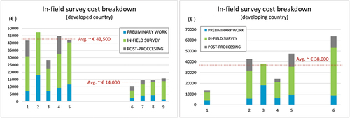
Now we can compare the two estimates. The costs entailed in carrying out a field survey are significantly higher than those derived from the use of remotely sensed data. The cost of the latter is estimated at €9,750, which is 70% of the average for the group of lower estimates (€13,915) and only 22% compared to the highest average (€43,575). As for the developing country scenario, the cost of a remote sensing survey would be the same, €9,750, and represents 25% of the estimate for a field survey (€38,336).

These results seems to show that the use of remote sensing allows for reducing the cost of an exposure and seismic vulnerability evaluation considerably.

Conclusions and proposal of a combined approach

In the present paper, we have shown that it is possible to generate an exposure and vulnerability database for 21 sample areas in the city of Port Prince using freely available aerial orthophotos and LiDAR. To do so, various spatial analysis methods and machine learning techniques were used to extract and classify data about 6,000 buildings, which were then assigned a vulnerability model. The seismic risk results obtained using this database prove its technical and economic feasibility.

Regarding the technical aspects of the methodology, we can conclude that:

1. Using a stratified approach, even though is not common in the literature, enables to parameterize the processes of analysis specifically for each urban pattern and allows for a better understanding of the results and the errors.

2. Manually digitizing building footprints has proven to be a highly accurate and relatively fast process, as we were able to digitize between 5 and 13 buildings per minute (including labeling the roofing material). In contrast, footprints obtained using semi-automated OBIA processes have consistently produced worse results. However, these results are also valid and have a clear advantage: automated processes are faster and more suitable for analyzing large areas.

3. Typically, OBIA processes are carried out using only spectral bands derived from images. This study includes two bands created using LiDAR (height and intensity) that have proven to be very useful in obtaining high accuracies when detecting roofs and roofing material (F1-Score of 95% and 99%).

4. Building typologies were identified based mainly on the attributes roof height and roofing material. Creating predictive models with very few building attributes is a major advantage of remote sensing methods for MBT identification. However, the classification of the building stock in two MBT (RC and MAndW) is limited and should be extended upon future work. Also, it is advisable to include the year of construction as an attribute in the exposure database to inform about the condition of the buildings.

5. The most efficient classifier was the one created using SVM with a PUK kernel. The classifier reached overall accuracies between 74% and 88%, depending on the urban pattern. To the best of our knowledge, the PUK kernel has not been used in this field of application. Despite these promising results, Port Prince is a singular scenario where the presence of metal roofs in both reinforced concrete buildings and masonry dwellings makes it difficult for predictive models to accurately distinguish between these two building types. This results in a slight overestimation of the number of masonry buildings, which is likely the main source of uncertainty in this study. It is a prediction error that should be addressed and minimized.

As for the feasibility analysis of the methodology, we can conclude that:

1. The seismic exposure and vulnerability databases obtained using semi-automated processes are technically feasible for calculating seismic risk. Comparing these results with those obtained using vulnerability data gathered in the field (CNIGS DB) resulted in a MAPE of 7.55% for the damage estimate using the footprints obtained using OBIA automated processes, and 3.78% for the manually digitized footprints. These low error rates seem to indicate that the uncertainties accumulated throughout the building detection and seismic vulnerability evaluation process did not significantly influence the final step of damage assessment, which means that it is possible to get high accuracies when estimating earthquake damage in a complex scenario, such as the city of Port Prince. In other words: the accuracy of these results seems to prove the reliability of using exposure and vulnerability databases created with remote sensing and machine learning in seismic risk studies.

2. Regarding economic feasibility, we found that conducting a seismic vulnerability study using remote sensing could reduce costs by between 30% and 78% with respect to the cost of a field survey. In addition to being considerably less expensive, the remote sensing study may be scaled exponentially without incurring significantly higher costs. If we compare the estimated periods required to perform each job, we see that the remote sensing study would only take between 13% and 60% of the time estimated for an in-field building inspection.

In light of these results, it seems possible to conclude that creating seismic exposure and vulnerability databases using remote sensing is feasible and cost-efficient in both developed and developing countries.

Finally, after carrying out this research, it may seem obvious to propose remote sensing rather than traditional field campaigns, as the most appropriate way to analyze vulnerability in cities. However, we believe that the best option is a combination of the two, in which an interdisciplinary team of experts in Civil Engineering, Architecture, and Engineering/Data Science could work together, as pointed out by the scientific community (e.g. Taubenböck et al. 2009; Wieland 2013; Stepinac and Gasparovic 2020). To this end, we propose a process composed of five key phases:

1. A preliminary qualitative study of the city using satellite, aerial, or terrestrial images. Several free sources are available for this purpose: Landsat, ASTER-GDEM, PNOA, Sentinel, Google Earth, Google Street View …

2. Stratifying the city into homogeneous urban patterns according to the size and layout of its buildings, the width and regularity of the road network, the presence of vegetation, the approximate age of the buildings, etc.

3. Generating Building Footprints. This can be done by consulting official sources where these have already been generated (cadaster, census, statistics institute, etc.) or other sources such as OSM. If no such sources are available, the footprints need to be digitized or obtained by segmenting high-resolution images. This will likely require acquiring data from optical images and 3D information (LiDAR or Radar).

In this step, a decision is made about whether a field campaign for sampling is necessary.

• (4) If it is determined to be necessary, the campaign would be designed based on all the information obtained in the previous steps. The survey would not be carried out to collect information about every building, but only about buildings in a particular part of the city (due to the difficulty of identifying a certain typology with remote sensing or applying analysis techniques in a specific area) that would be determined in advance. This allows for considerable cost savings and optimized planning.

• (5)Calculating footprint attributes and applying predictive models for classifying building typology. Finally, each typology is assigned a vulnerability model.

The product derived from this procedure would be a highly accurate exposure and vulnerability database for the city created by combining remote sensing analysis with a targeted field survey, thereby optimizing costs and time. This would be consistent with the above-mentioned Sendai Framework objectives regarding expanding the number of countries, especially developing countries, which analyze seismic risk to propose DRR measures. This is, in turn, in line with the SDG nr. 11.B. In addition, it would promote the use of open-access data sources, which, far from being a detriment to any country, contributes to its development and international positioning. By making their data available, countries would help minimize the difficulties that lack of information poses to understanding risk, as the UN has pointed out.

Acknowledgments

The present research has been developed in the framework of a PhD Thesis and in parallel with the SISMO-HAITI series of projects, both funded by the Universidad Politécnica de Madrid (UPM). We want to thank the Haitian Ministère des Travaux Publics, Transports et Communications; the OpenTopography repository; Don McKeown and Nina Raqueno (from the Rochester Institute of Technology); and Christina Corbane (from the European Commission’s Joint Research Centre) for kindly contributing all the data needed to accomplish this study. Also, we want to thank the twelve international experts that helped with the cost estimation of the field survey (in alphabetic order): Jorge Gaspar-Escribano, Dimitra Kalantoni, Dominik Lang, Francisco Martínez, Sandra Martínez, Abdelghani Meslem, Sergio Molina, Massimiliano Pittore, Antonios Pomonis, Ligia Quirós, Robin Spence y Marc Wieland.

Authors also thank the four anonymous reviewers that contributed to improve this paper.

Disclosure statement

No potential conflict of interest was reported by the author(s).

Data availability statement

Part of the data (LiDAR point clouds) that support the findings of this study are available in the public domain at https://www.opentopography.org/. The rest of the datasets (ortho-imagery and building databases) have been provided for this study by third parties and authors have no authorization to share them. References to data providers are given in the text, in the section Materials And Methods. The template of the form that experts filled-in to evaluate the cost of an in-field survey is shared in Mendeley Data with the name “Template – Building In-Field Survey”.

Additional information

Funding

The work was supported by the Universidad Politécnica de Madrid [-];European Institute of Innovation and Technology (EIT) [-];

References

- SDG-United Nations: https://sdgs.un.org/goals/goal11. Accessed 24/12/2023
- Arredondo, A. 2019. GitHub repositoy. Haiti OBIA. https://github.com/arredond/haiti-obia.
- Bhattacharjee, A., and R. Lossio. 2011. “Evaluation of OCHA Response to theHaiti Earthquake.” Final Report January.
- Bilham, R. 2010. “Lessons from the Haiti Earthquake.” Nature 463 (7283): 878–33. doi:10.1038/463878a.
- Bittner, K., F. Adam, S. Cui, M. Koerner, and P. Reinartz. 2018. “Building Footprint Extraction from VHR Remote Sensing Images CombinedWith Normalized DSMs Using Fused Fully Convolutional Networks.” Ieee Journal ofSelected Topics in Applied Earth Observations and Remote Sensing 11 (8): 2615–2629. doi:10.1109/jstars.2018.2849363.
- Boore, D. M., J. P. Stewart, E. Seyhan, and G. M. Atkinson. 2014. “NGA-West2 Equations for Predicting PGA, PGV, and 5% Damped PSA for ShallowCrustal Earthquakes.” Earthquake Spectra 30 (3): 1057–1085. doi:10.1193/070113eqs184m.
- Borfecchia, F., M. Pollino, L. De Cecco, A. Lugari, S. Martini, L. La Porta, E. Ristoratore, and C. Pascale. 2010. “Active and Passive Remote Sensing for Supporting The evaluation of the Urban Seismic Vulnerability.” Rivista Italiana Di Telerilevamento 42 (3): 129–141. doi:10.5721/ItJRS201042310.
- Breiman, L. 2001. “Random Forests.” Machine Learning 45 (1): 5–32. doi:10.1023/a:1010933404324.
- Cerri, M. 2018. “Multivariable Flood Damage Modelling for Residential Buildings using Open Data with Random Forests.“ Technische Universität München. 82. https://elib.dlr.de/125790/.
- Chiou, B. S. J., and R. R. Youngs. 2014. “Update of the Chiou and Youngs NGAModel for the Average Horizontal Component of Peak Ground Motion andResponse Spectra.” Earthquake Spectra 30 (3): 1117–1153. doi:10.1193/072813eqs219m.
- Corbane, C., K. Saito, L. Dell’oro, E. Bjorgo, S. P. D. Gill, B. Piard, C. K. Huyck, et al. 2011. “A Comprehensive Analysis of Building Damage in the 12 January 2010 M(W)7 Haiti Earthquake Using High-Resolution Satellite- and Aerial Imagery.” Photogrammetric Engineering & Remote Sensing 77 (10): 997–1009. doi:10.14358/pers.77.10.0997.
- Costanzo, A., A. Montuori, J. Pablo Silva, M. Silvestri, F. D. MassimoMusacchio, S. Stramondo, M. Fabrizia Buongiorno, and M. Buongiorno. 2016. “The Combined Use of Airborne Remote Sensing Techniques Within a GISEnvironment for the Seismic Vulnerability Assessment of Urban Areas: AnOperational Application.” Remote Sensing 8 (2): 146. doi:10.3390/rs8020146.
- Cox, B. R., J. Bachhuber, E. Rathje, C. M. Wood, R. Dulberg, R. A. G. AlbertKottke, S. M. Olson, and S. M. Olson. 2011. “Shear Wave Velocity- andGeology-Based Seismic Microzonation of Port-Au-Prince, Haiti.” EarthquakeSpectra 27 (1_suppl1): S67–92. doi:10.1193/1.3630226.
- CRED, UNISDR. 2016. “Poverty & Death: Disaster Mortality, 1996–2015.” In Centre for Research on the Epidemiology of Disasters, Brussels, Belgium.
- Dell’acqua, F., P. Gamba, and K. Jaiswal. 2013. “Spatial Aspects of Building And population Exposure Data and Their Implications for Global Earthquake Exposure Modeling.” Natural Hazards 68 (3): 1291–1309. doi:10.1007/s11069-012-0241-2.
- De Los Santos, M. J. D., and J. A. Principe. 2021. “Gis-Based Rapid Earthquake Exposure and Vulnerability Mapping Using Lidar Dem and Machine Learning Algorithms: Case of Porac, Pampanga.” International Archives of the Photogrammetry, Remote Sensing & Spatial Information Sciences 46, 17–19 November 2021.
- Dustin, M., T. Kijewski-Correa, and A. A. Taflanidis. 2011. “Assessment of Residential Housing in Léogâne, Haiti, and Identification of Needs for Rebuilding After the January 2010 Earthquake.” Earthquake Spectra 27 (1_suppl1): S299–322. doi:10.1193/1.3637942.
- Eberhard, M. O., S. Baldridge, J. Marshall, W. Mooney, and G. J. Rix. 2010. “The Mw 7.0 Haiti Earthquake of January 12, 2010: USGS/EERI Advance reconnaissance Team Report.” US Geological Survey Open-File Report 1048 (2013). doi: https://pubs.usgs.gov/of/2010/1048/.
- Ehrlich, D., T. Kemper, X. Blaes, and P. Soille. 2013. “Extracting Building Stock information from Optical Satellite Imagery for Mapping Earthquake Exposure And its Vulnerability.” Natural Hazards 68 (1): 79–95. doi:10.1007/s11069-012-0482-0.
- Fan, X., G. Nie, C. Xia, and J. Zhou. 2021. “Estimation of Pixel-Level Seismic Vulnerability of the Building Environment Based on Mid-Resolution Optical Remote Sensing Images.” International Journal of Applied Earth Observation and Geoinformation 101: 102339. doi:10.1016/j.jag.2021.102339.
- Fawcett, T. 2006. “An Introduction to ROC Analysis.” Pattern Recognition Letters 27 (8): 861–874. doi:10.1016/j.patrec.2005.10.010.
- Felzenszwalb, P. F., and D. P. Huttenlocher. 2004. “Efficient Graph-Based Imagesegmentation.” International Journal of Computer Vision 59 (2): 167–181. doi:10.1023/b:visi.0000022288.19776.77.
- FEMA-178. 1992. “NEHRP Handbook for the Seismic Evaluation of Existing Buildings”. FEMA 178, Federal Emergency Management Agency, Washington, D.C., USA.
- FEMA-440. 2005. “Improvement of Nonlinear Static Seismic Analysis Procedures”. FEMA 440, Federal Emergency Management Agency, Washington D.C.
- Fierro, E., and C. Perry. 2010. “Preliminary Reconnaissance Report.” BFP Engineers 12. January 12, 2010. https://apps.peer.berkeley.edu/publications/haiti_2010/documents/Haiti_Reconnaissance.pdf.
- GAR. 2009. “Global Assessment Report on Disaster Risk Reduction”. United Nations International Strategy for Disaster Reduction Secretariat (UNISDR). ISBN/ISSN: 9789211320282. 207pp
- Geiss, C., P. Aravena Pelizari, M. Marconcini, W. Sengara, T. L. MarkEdwards, H. Taubenboeck, and H. Taubenböck. 2015. “Estimation of Seismic building Structural Types Using Multi-Sensor Remote Sensing and Machine Learningtechniques.” ISPRS Journal of Photogrammetry and Remote Sensing 104: 175–188. doi:10.1016/j.isprsjprs.2014.07.016.
- Geiss, C., M. Jilge, T. Lakes, and H. Taubenboeck. 2016. “Estimation of Seismic Vulnerability Levels of Urban Structures with MultisensorRemote Sensing.” Ieee Journal of Selected Topics in Applied Earth Observations and Remote Sensing 9 (5): 1913–1936. doi:10.1109/jstars.2015.2442584.
- Geiss, C., A. Schauss, T. Riedlinger, S. Dech, C. Zelaya, M. A. H. NicolasGuzman, J. Jokar Arsanjani, H. Taubenboeck, and H. Taubenböck. 2017. “Joint Use of Remote Sensing Data and Volunteered Geographic Information for Exposure Estimation: Evidence from Valparaíso, Chile.” Natural Hazards 86 (86): 81–105. doi:10.1007/s11069-016-2663-8.
- Grünthal, G. 1998. European Macroseismic Scale 1998. In: European Seismological Commission (ESC).
- Guiwu, S., Q. Wenhua, S. Zhang, T. Sim, X. Liu, R. Sun, L. Sun, and Y. Jin. 2015. “An Integrated Method Combining Remote Sensing Data andLocal Knowledge for the Large-Scale Estimation of Seismic Loss Risks to Buildings in the Context of Rapid Socioeconomic Growth: A Case Study in Tangshan,china.” Remote Sensing 7 (3): 2543–2601. doi:10.3390/rs70302543.
- Hancilar, U., F. Taucer, and C. Corbane. 2013. “Empirical Fragility Functions based on Remote Sensing and Field Data After the 12 January 2010 HaitiEarthquake.” Earthquake Spectra 29 (4): 1275–1310. doi:10.1193/121711eqs308m.
- Hao, W., Z. Cheng, W. Shi, Z. Miao, and X. Chenchen. 2014. “An object-Based Image Analysis for Building Seismic Vulnerability Assessment Using high-Resolution Remote Sensing Imagery.” Natural Hazards 71 (1): 151–174. doi:10.1007/s11069-013-0905-6.
- Hayes, G. P., E. K. Meyers, J. W. Dewey, R. W. Briggs, P. S. Earle, H. M. Benz, G. M. Smoczyk, H. E. Flamme, W. D. Barnhart, and R. D. Gold. 2017. Tectonic Summaries of Magnitude 7 and Greater Earthquakes from 2000 to 2015. In: US Geological Survey.
- Kononenko, I. 1994. Estimating Attributes: Analysis and Extensions of RELIEF. Paperpresented at the European conference on machine learning, Catania, Italy, April 6–8, 1994.
- Lagomarsino, S., and S. Giovinazzi. 2006. “Macroseismic and Mechanical Models for the Vulnerability and Damage Assessment of Current Buildings.” Bulletin of Earthquake Engineering 4 (4): 415–443. doi:10.1007/s10518-006-9024-z.
- Lallemant, D. 2014. “Waiting for the Big One: The Continued Earthquake Risk of Port-Au-Prince, Haiti”. In 3rd International Conference on Urban Disaster Recovery at Boulder, Colorado. DOI: 10.13140/2.1.2057.8087
- Landis, J. R., and G. G. Koch. 1977. “Measurement of Observer Agreement For categorical Data.” Biometrics 33 (1): 159–174. doi:10.2307/2529310.
- Liuzzi, M., P. Aravena Pelizari, C. Geiss, A. Masi, V. Tramutoli, and H. Taubenboeck. 2019. “A Transferable Remote Sensing approach to Classify Building Structural Types for Seismic Risk Analyses: The Case ofVal d’Agri Area (Italy).” Bulletin of Earthquake Engineering 17 (9): 4825–4853. doi:10.1007/s10518-019-00648-7.
- Milutinovic, Z. V., and G. S. Trendafiloski. 2003. “Risk-UE An advanced approach to earthquake risk scenarios with applications to different european towns.” In Contract: EVK4-CT-2000-00014, 1–111. WP4: Vulnerability of Current Buildings. http://www.civil.ist.utl.pt/~mlopes/conteudos/DamageStates/Risk%20UE%20WP04_Vbility.pdf.
- Molina, S., D. H. Lang, and C. D. Lindholm. 2010. “SELENA - An Open-Source Tool For seismic Risk and Loss Assessment Using a Logic Tree Computation procedure.”Computers &.” Geosciences 36 (3): 257–269. doi:10.1016/j.cageo.2009.07.006.
- Molina, S., Y. Torres, B. Benito, M. Navarro, and D. Belizaire. 2014. “Using the Damage from 2010 Haiti Earthquake for Calibrating Vulnerability Models of Typical structures in Port-Au-Prince (Haiti).” Bulletin of Earthquake Engineering 12 (4): 1459–1478. doi:10.1007/s10518-013-9563-z.
- Moya, L., C. Geis, M. Hashimoto, E. Mas, S. Koshimura, and G. Strunz. 2021. “Disaster Intensity-Based Selection of Training Samples for Remote Sensing Building Damage Classification.” IEEE Transactions on Geoscience and Remote Sensing 59 (10): 8288–8304. doi:10.1109/tgrs.2020.3046004.
- MTPTC 2010. “Evaluation des Batiments”. In: Ministere des Travaux Publics, Transports et Communications. http://www.mtptc.gouv.ht/accueil/actualites/article_7.html. Accessed 17/03/2022.
- Mueck, M., H. Taubenboeck, J. Post, S. Wegscheider, G. Strunz, S. Sumaryono, and F. A. Ismail. 2013. “Assessing Building Vulnerability to Earthquake and Tsunami Hazard using Remotely Sensed Data.” Natural Hazards 68 (1): 97–114. doi:10.1007/s11069-012-0481-1.
- Panagiota, M., C. Jocelyn, P. Erwan, G. Philippe, and Ieee.2012. “A Support Vector Regression Approach for Building Seismic vulnerability Assessment and Evaluation from Remote Sensing Andin-Situ Data.” 2012 Ieee International Geoscience and Remote SensingSymposium (Igarss):7533–7536. doi: 10.1109/igarss.2012.6351888.
- Pittore, M., and M. Wieland. 2013. “Toward a Rapid Probabilistic Seismic vulnerability Assessment Using Satellite and Ground-Based Remote sensing.”Natural Hazards.” Natural Hazards 68 (1): 115–145. doi:10.1007/s11069-012-0475-z.
- Polli, D., and F. Dell’acqua. 2011. “Fusion of Optical and SAR Data for SeismicVulnerability Mapping of Buildings.” Optical Remote Sensing: Advances in SignalProcessing and Exploitation Techniques 3: 329–341. doi:10.1007/978-3-642-14212-3_15.
- Quinlan, J. R. 1993. C4.5: Programs for Machine Learning. San Mateo, CA: Morgan Kaufmann Publishers.
- Riedel, I., P. Gueguen, M. Dalla Mura, E. Pathier, T. Leduc, and J. Chanussot. 2015. “Seismic Vulnerability Assessment of Urban environments in Moderate-To-Low Seismic Hazard Regions Using Association Rule learning and Support Vector Machine Methods.” Natural Hazards 76 (2): 1111–1141. doi:10.1007/s11069-014-1538-0.
- Riedel, I., P. Gueguen, F. Dunand, and S. Cottaz. 2014. “Macroscale VulnerabilityAssessment of Cities Using Association Rule Learning.” Seismological ResearchLetters 85 (2): 295–305. doi:10.1785/0220130148.
- Ruggieri, S., A. Cardellicchio, V. Leggieri, and G. Uva. 2021. “Machine-Learning Based Vulnerability Analysis of Existing Buildings.” Automation in Construction 132: 103936. doi:10.1016/j.autcon.2021.103936.
- Sarabandi, P., A. Kiremidjian, R. T. Eguchi, and B. J. Adams. 2008. “Building Inventory Compilation for Disaster Management: Application of Remote sensing and Statistical Modeling.“ Technical Report Series MCEER-08-0025. 132. Buffalo: MCEER. https://www.eng.buffalo.edu/mceer-reports/08/08-0025.pdf .
- Shunping, J., S. Wei, and L. Meng. 2019. “Fully Convolutional Networks forMultisource Building Extraction from an Open Aerial and Satellite Imagery DataSet.” IEEE Transactions on Geoscience and Remote Sensing 57 (1): 574–586. doi:10.1109/tgrs.2018.2858817.
- Silva, V., P. Henshaw, C. Huyck, and M. O’hara. 2018. “GED4ALL Global Exposure Database for Multi-Hazard Risk Analysis D5-FINAL REPORT.” In.: GEM Technical Report 2018-05. Pavia: GEM Foundation.
- Sohn, G., and I. Dowman. 2007. “Data Fusion of High-Resolution Satellite Imagery and LiDar Data for Automatic Building Extraction.” Isprs Journal ofPhotogrammetry and Remote Sensing 62 (1): 43–63. doi:10.1016/j.isprsjprs.2007.01.001.
- Stepinac, M., and M. Gasparovic. 2020. “A Review of Emerging Technologies for an Assessment of Safety and Seismic Vulnerability and Damage Detection of Existing Masonry Structures.” Applied Sciences-Basel 10 (15): 5060. doi:10.3390/app10155060.
- Symithe, S., and E. Calais. 2016. “Present-Day Shortening in Southern Haiti fromGps Measurements and Implications for Seismic Hazard.” Tectonophysics 679 (679): 117–124. doi:10.1016/j.tecto.2016.04.034.
- Taubenböck, H., A. Roth, S. Dech, H. Mehl, J. C. Münich, L. Stempniewski, and J. Zschau. 2009. “Assessing Building Vulnerability Using Synergistically Remotesensing and Civil Engineering.” In Urban and Regional Data Management, edited by Alenka Krek, Massimo Rumor, Sisi Zlatanova, Elfriede M. Fendel, 299–312. London: CRC Press.
- Template - Building In-Field Survey. Torres, Yolanda (2022). Mendeley Data, V2, doi: 10.17632/rgmtgdnkjb.2
- Torres, Y., S. Molina, S. Martinez-Cuevas, M. Navarro, J. J. Martinez-Diaz, B. Benito, J. J. Galiana-Merino, and D. Belizaire. 2016. “A First Approach to Earthquake damage Estimation in Haiti: Advices to Minimize the Seismic Risk.” Bulletin ofEarthquake Engineering 14 (1): 39–58. doi:10.1007/s10518-015-9813-3.
- Ustun, B., W. J. Melssen, and L. M. C. Buydens. 2006. “Facilitating the Application ofSupport Vector Regression by Using a Universal Pearson VII Function Basedkernel.” Chemometrics and Intelligent Laboratory Systems 81 (1): 29–40. doi:10.1016/j.chemolab.2005.09.003.
- Vapnik, V. 2000. “The Nature of Statistical Learning Theory”. 2nd ed. New York, NY, USA: Springer. doi:10.1007/978-1-4757-3264-1.
- Wenhua, Q., S. Guiwu, L. Sun, F. Yang, and W. Yang. 2017. ““Internet+” Approach to Mapping Exposure and Seismic Vulnerability of Buildings in a Context of Rapid Socioeconomic Growth: A Case Study in Tangshan, China.” Natural Hazards 86 (S1): 107–139. doi:10.1007/s11069-016-2581-9.
- Wieland, M. 2013. “Exposure Estimation for Rapid Seismic Vulnerability Assessment: An Integrated Approach Based on Multi-Source Imaging.“ PhD. Thesis, EWS Centre for EarlyWarning, Geoengineering Centres, GFZ Publication. https://doi.org/10.14279/depositonce-3844.
- Wieland, M., and M. Pittore. 2014. “Performance Evaluation of MachineLearning Algorithms for Urban Pattern Recognition from Multi-Spectral SatelliteImages.” Remote Sensing 6 (4): 2912–2939. doi:10.3390/rs6042912.
- Wieland, M., M. Pittore, S. Parolai, and J. Zschau. 2012. “Exposure Estimation from Multi-Resolution Optical Satellite Imagery for SeismicRisk Assessment.” ISPRS International Journal of Geo-Information 1 (1): 69–88. doi:10.3390/ijgi1010069.
- Wieland, M., M. Pittore, S. Parolai, J. Zschau, B. Moldobekov, and U. Begaliev. 2012. “Estimating Building Inventory for Rapid Seismic Vulnerability Assessment: Towards an Integrated Approach Based on Multi-Source Imaging.” Soil Dynamics andEarthquake Engineering 36: 70–83. doi:10.1016/j.soildyn.2012.01.003.
- Wieland, M., Y. Torres, M. Pittore, and B. Benito. 2016. “Object-Based Urban Structure Type Pattern Recognition from Landsat TM with a SupportVector Machine.” International Journal of Remote Sensing 37 (17): 4059–4083. doi:10.1080/01431161.2016.1207261.
- Yolanda, T., J. Juan Arranz, J. M. Gaspar-Escribano, A. Haghi, B. B. SandraMartinez-Cuevas, J. Carlos Ojeda, and J. C. Ojeda. 2019. “Integration ofLidar and Multispectral Images for Rapid Exposure and Earthquake Vulnerability estimation. Application in Lorca, Spain.” International Journal of Applied EarthObservation and Geoinformation 81: 161–175. doi:10.1016/j.jag.2019.05.015.
- Yongyang, X., W. Liang, Z. Xie, and Z. Chen. 2018. “Building Extraction inVery High Resolution Remote Sensing Imagery Using Deep Learning and GuidedFilters.” Remote Sensing 10 (1): 144. doi:10.3390/rs10010144.
- Zhou, J., Y. Liu, G. Nie, H. Cheng, X. Yang, X. Chen, and L. Gross. 2022. “Building Extraction and Floor Area Estimation at the Village Level in Rural China via a Comprehensive Method Integrating UAV Photogrammetry and the Novel EDSANet.” Remote Sensing 14 (20): 5175. doi:10.3390/rs14205175.