LiDAR-change-based mapping of sediment movement from an extreme rainfall event

ABSTRACT

Mapping landscape change at fine scales (e.g. <1.0 m resolution) using airborne LiDAR data from manned aircraft is a significant challenge. This challenge is magnified in disaster response contexts. A combination of collection and processing factors contributes to horizontal and vertical errors (and resulting uncertainty) in each pre- and post-LiDAR derived digital elevation model (DEM). Subsequently, the errors in the change surface from the two (or more) DEMs are an accumulation of the errors in the individual DEMs. Thus, reliable mapping erosion/deposition changes at sub-meter precision in change detection studies using LiDAR data is largely the domain of terrestrial LiDAR or sUAS with LiDAR scanners rather than manned aircraft. Unfortunately, terrestrial and sUAS LiDAR scanners are not well suited for mapping large areas and sUAS collections are subject to additional airspace constraints compared to manned aircraft. In this study, we probed one of the significant issues in airborne LiDAR change projects – vertical height errors from sequential flight lines. A simplified solution for determining flight line vertical biases in areas of low topographic relief with natural cover types was developed and tested for normalizing point clouds. The approach was tested in a fine-scale erosion/deposition study from an extreme rainfall event that eroded and deposited sand at depths of about 1.0 m. Airborne LiDAR had been collected prior to the rainfall event, and another airborne LiDAR collection was made 1 month after the event. Eleven field campaigns to collect reference data and visit anomalies in the change surface were conducted in a 15-month period after the event, beginning 25 February 2016 and ending 8 May 2017. The validation results indicate accuracies for the pre-event and post-event LiDAR derived DEMs were 7.8 cm and 13.0 cm RMSE, respectively. After modeling vertical errors and corrections applied to the post-event point clouds, the RMSE for the post-event DEM was 8.3 cm. In the depositional use case, 27 locations were sampled with auger boreholes/sand pits and compared with LiDAR-based change. The LiDAR-based change detection analysis resulted in predicted sand depth accuracies of 94% with a mean error of 4.7 cm.

KEYWORDS:

• LiDAR
• change detection
• flood
• sand deposition
• military training area

1. Introduction

Mapping landscape change at fine scales (e.g. <1.0 m resolution) using airborne LiDAR data from manned aircraft is a significant challenge, as compared to sUAS-based systems, as the collection heights are typically above 1000 m and at higher velocities. A combination of collection and processing factors contributes to horizontal and vertical errors (and resulting uncertainty) in each pre- and post-LiDAR derived DEM. Subsequently, the errors in the change surface from the two (or more) digital elevation models (DEMs¹) are an accumulation of the errors in the individual DEMs. Thus, reliable mapping erosion/deposition changes at sub-meter precision in change detection studies using LiDAR data is largely the domain of terrestrial LiDAR or sUAS with LiDAR scanners rather than manned aircraft. Unfortunately, terrestrial and sUAS LiDAR scanners are not well suited for mapping large areas and are subject to additional airspace constraints compared to manned aircraft.

Sources of horizontal and vertical error in LiDAR point clouds can originate from sensor/collection (e.g. bore-sight, global navigation satellite system (GNSS) control, INS interpolation and atmospheric stability, etc.), pointing angles to surfaces (e.g. surface cover types, topographic orientation angles, etc.), and post-processing approaches (e.g. waveform-to-return classification, return labeling into land cover types, interpolation to a DEM, etc.). The observable errors in LiDAR-derived positions are derived from multiple error sources, some correlated and some independent. For most applications, the sources of errors and their interdependencies are unknown although attempts at modeling the errors in error-budget modeling have been made (Hodgson and Bresnahan 2004). Considerable research in the application of LiDAR-derived data to a specific domain has attempted to remove or minimize dominant error sources, ignoring the lesser important or at least the unknown errors, prior to the application problem. Some dominant error sources can be visually noticed, and sources inferred, such as the bore-sight problem and GNSS bias. Of these composite error sources, the most notable is from horizontal and/or vertical differences from overlapping LiDAR flightlines (often called “strips”). Vendor solutions have ranged from simply removing LiDAR points from only one flightline so the consumer does not notice the differences (Schuckman, Earth Data, pers. comm., 1999) to attempts at minimizing measurable errors prior to distribution of a product. For the notable horizontal and height anomalies, many researchers utilizing the data for applications focus attention on notable and perhaps, dominant causal factors associated with differences between flight lines; thus, attempting from simple to somewhat intensive approaches in what is referred to as strip-adjustment solutions.

Some have categorized strip adjustment approaches as either system-driven or data-driven (Chen, Li, and Yang 2021). System-driven approaches focus on correcting errors in the sensor, mounting, GNSS trajectory, etc. and are typically only conducted by the vendor or data collector as they have access to all parameter/values. Data-driven approaches are often the focus by the application user community who typically only have access to the point-cloud or subsequent data products. Data-driven approaches can also be categorized based on reference or correlate data, such as ground reference observations (“marker-based”) identified by the analyst versus automated approaches using natural features (“marker-free”) alone (Fekry et al., 2021). Reference data, such as building corners (Rentsch and Krzystek 2012; Zhang et al., 2015) or pavement lines (Toth and Grejner-Brzezinska 2009), can be identified by the analyst. Natural features for automated strip adjustment can be terrain features (Chen, Li, and Yang 2021; Favalli, Fornaciai, and Pareschi 2009; Glira et al., 2015) or forest canopy (Fekry et al., 2021). Methods based on terrain features assume that airborne LiDAR point cloud has been adequately classified into “bare earth” points versus non-bare earth points or for satellite imagery over unvegetated areas, such as glacial landscapes (Nuth and Kääb 2011).

To place our study area application and strip adjustment approach in context, we present a few previous research examples to illuminate the differences in reference data, terrain type, and the constraints. Toth and Grejner-Brzezinska (2009) provided a novel approach for identifying reflective “targets,” such as pavement markings, along roadways to use as ground control in a strip adjustment. Unfortunately, for a heavily vegetated area with only sand roads, the nicely paved roadways for reference targets are non-existent.

Chen, Li, and Yang (2021) developed a “DEM-Iterative Closest Point” approach for strip adjustment of UAV-borne LiDAR data in mountainous terrain that uses terrain features rather than anthropogenic features. Differences between adjacent strips were reduced from about 1.5 m to 0.35 m meters. However, as noted by the authors, their method would not work well in areas of low local relief (Chen, Li, and Yang 2021). Favalli, Fornaciai, and Pareschi (2009) also developed a strip adjustment approach based on natural features in the terrain for a change detection study of Mt. Etna. Their method determined both horizontal and vertical differences in overlapping strips. The problem context of flat areas with strip adjustment methods was also noted by the authors.

The present study is the development and application of a change detection approach that requires strip adjustment and geographic/geomorphic interpretation of anomalies, anomalies for which we have no automated method of correction. The study area is of low topographic relief with gradually changing slopes on an almost exclusive natural environment with sand roads. Moreover, the topographic changes we are interested in are less than 1.0 m. It is useful to note that the technology typically implemented with manned aircraft LIDAR sensors is considerably more precise and accurate than UAV-borne LiDAR sensors. However, manned aircraft typically fly at much higher altitudes (e.g. 1000 m and above), while UAV LiDAR missions are generally restricted to altitudes lower than 120 m. Such low altitudes typically result in much higher accuracies in both the vertical and horizontal domain and much denser point clouds. However, UAV-borne sensors are typically controlled by much less precise and accurate inertial measurement units (IMUs), inertial navigation system (INS), lower-powered lasers, etc. It is also important to note that these technologies have evolved over the last 25 years (and continue to evolve, particularly with UAV-borne LiDAR). For example, the update frequency of GNSS sensors used to determine the aircraft position (and sensor) and orientation has increased dramatically. The INSs used for the typical manned airborne LiDAR units are often ten times the cost of a complete UAV system alone. The IMUs are export controlled. Thus, a systematic review of the strip adjustment literature must consider the evolving nature of the entire technology (e.g. platform, GNSS, IMU, INS, laser), the collection environment (e.g. topography, land cover, contract requirements/disaster response), and the post-processing approaches (e.g. waveform and return determination, return labeling). Such an exhaustive and comparative review is beyond the scope of this paper.

In this paper, we focus on a relatively simple data-driven strip-adjustment approach, supported by reference observations in the field, to map fine-scale topographic changes from a historic rainfall event using manned airborne LiDAR missions. The study area context is an area of low to modest local relief, almost completely covered by evergreen/mixed forests with a few open fields, interspersed by sand roads and firebreaks. The change event was a “500-year rainfall event.” The post-event collection was a rapidly organized manned airborne flyover 41 days after the rainfall event. The LiDAR data collections were unique to the interests of the U.S. Army and South Carolina National Guard and, moreover, were unique because of a catastrophic flood event. These LiDAR collections should not be confused with the nationwide efforts of the USGS and FEMA for their interests, such as flood plain mapping, and do not adhere to the well-known “Q*” collection/processing requirements (e.g. Q level 1, Q level 2, etc.) stipulated in the USGS guidelines for LiDAR collections and post-processing (USGS 2022). However, the LiDAR collections in this study are symbolic of the rapidly organized and executed disaster response applications of airborne LiDAR data. The nature of and management of sand roads on a military reservation is a different challenge than the road management in public spaces. First, the roads are meant to be passable by four-wheel drive vehicles but not necessarily two-wheel drive vehicles. Second, the sand roads on a military reservation are designed to be functional for military day/night training but are not expected to be in perfect condition.

The unprecedented rainfall event of October 2015 resulted in widespread damage to the sand roads on the McCrady Training Center (MTC) in South Carolina. In 2 days (October 3^rd and 4^th), over 55 cm (21.6 inches) of rainfall was recorded at the meteorological station on the MTC. In the meteorological context, this October 2015 rainfall event was considered a 500-year rainfall event. The sand roads were heavily eroded and the material displaced and moved onto both parts of the road and nearby landscape. The same rainfall event impacted the central portion of South Carolina causing over 50 small earthen dams to fail. In the context of understanding what/why the large magnitude erosion/deposition occurred and how to plan for mitigating before a future possible large storm event, the applicative research questions posed immediately after this catastrophic rainfall event were:

• Where were the erosive and depositional areas?

• What magnitude of erosion/deposition occurred?

• How confident are the mapped erosion/deposition areas?

• What factors influence the confidence in mapping erosion/deposition?

To answer these questions we utilized pre- and post-LiDAR from manned airborne data collections to map erosion/depositional areas. However, to map vertical surface changes at precisions less than 1.0 m a common, but often ignored, bias in LiDAR data caused by multiple flightlines was probed and minimized. An approach was developed to detect and quantify vertical biases by flightline. Additionally, five unique anomalies associated with fine-scale surface changes were identified from field visits and presented.

Related to our applicative research questions, in this paper we focus on two important methodological questions:

• How well will a simplistic data-driven strip-adjustment approach work for a modest local relief natural landscape?

• What level of confidence can be obtained using this approach for a change detection?

Numerous studies have employed remote sensing approaches, particularly airborne or terrestrial LiDAR, to monitor continual soil erosion or even episodic events like landslides or volcanic events (Brasington, Langham, and Rumsby 2003; Challis et al., 2011; Eagleston and Marion 2020; James et al., 2012; Nourbakhshbeidokhti et al., 2019; Tseng et al., 2013). However, few studies using manned airborne LiDAR remote sensing methods have been applied to large areas at a fine detection resolution (i.e. 20 to 100 cm) (Pelletier and Orem 2014). This study presents both the findings and unique issues experienced with this unusual change detection event using manned airborne LiDAR missions. Attempting to detect and map fine vertical changes from LiDAR missions at higher altitudes requires careful examination of systematic horizontal and vertical biases in the point clouds that may be corrected. In this paper, we provide a practical solution for detecting systematic vertical biases by flight line and correct for the biases. Using in situ reference data, both unchanged and changed surface locations, we validated the resulting changed detection maps illustrating sediment erosion depositions.

We also include observations and discussion of five false erosion/depositional artifacts (less than 1 m) that may be present in other LiDAR-based change detection studies of major precipitation events. We are unaware of three of these artifacts ever being presented in the science literature.

2. Study area

Roads on the South Carolina Army National Guard’s MTC are almost exclusively sand. The MTC (Figure 1), co-located on the Fort Jackson Military Reservation, is 6,036 ha of rolling topography with small perennial and intermittent creeks incised into 1 to 2 m of sandy topsoil. Military buildings and housing are concentrated in the southeastern portion of the MTC and, with the exception of a 4 mile section of paved road just outside the east boundary and most southern boundary around operational buildings, all other roads are composed of sandy soils. The bulk of the training site is a former agricultural landscape where the products were primarily turpentine, logging, and subsistence agriculture with a few moonshine stills. The only expansive crop was cotton farming. The remains of terraces abound throughout the low slopes and present in historic imagery as well as noticed in the DEMs produced from LiDAR data. Today the landscape is dominated by evergreen forests with scattered hardwood trees.

Figure 1. McCrady Study area for research project showing DEM and major hydrography. The three case studies mentioned in the text are also shown.

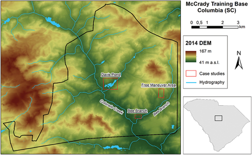
The typical ditches paralleling roads are common but never with protection strategies such as guardrails. A series of firebreak roads run east-west across the MTC, spaced approximately 180 m apart. The goal is to manage the sand roads in a manner to make them sustainable and operational for military training exercises.

2. Background

2.1 Airborne lidar-based change detection issues

There are numerous sources that limit the precision or introduce error in the airborne LiDAR collection/processing/terrain modeling approach. Foremost among these sources are the flying altitude, resulting spatial density of emitted pulses, GNSS control of sensor position and orientation, return classification into ground/non-ground, and interpolation algorithm for DEM construction. Except for the GNSS control in the actual sensor position/orientation, most other internal procedures conducted by the aeroservice vendor are rarely presented even to the funding client. The vendor will typically conduct an accuracy assessment using ground reference data and other methods for assessing consistency, depending on the contract and collection/processing specifications. Few of these limiting sources have been addressed in the literature.

The challenge in mapping changes in a topographic surface is determining what is an actual surface change from the apparent change caused by errors in the measurement methods. Mapping elevational changes using airborne LiDAR typically involves creation of a pre- and post-DEM and then subtracting the two DEMs (e.g. subtracting the pre-DEM from the post-DEM) to determine positive and negative elevational changes. However, the approach for collecting, post-processing, and analysis of such DEMs has limited precision and accuracy; thus, there are always elevational differences of some magnitude at each cell in the DEM. Simply stated, precision is the level of detail, such as the number of significant digits, in the measurement. Rounding elevation values to the whole meter would only provide a precision of 1 m while rounding to the nearest cm provides cm level precision. However, fine precision does not imply that the measurement is accurate. Thus, accuracy metrics, such as root mean squared error (RMSE), are often used to describe the accuracy of a dataset. Given an understanding of the precision and accuracy of each elevation surface model, the problematic question is what magnitude of elevational difference is a real surface change rather than an artifact of the LiDAR-based approach? This is a historic problem with the use of digital approaches in geomorphology.

Several authors have proposed methods for detecting or minimizing false changes, such as the classical approach expressed elegantly from geomorphology applications by Lane, Westaway, and Murray Hicks (2003). These methods include a threshold of confidence, expressed as a t-statistic or more commonly simply using the common 95% threshold (Wheaton et al., 2009), fuzzy logic (Wheaton et al. Cavalli et al., 2017; Wheaton et al., 2009), and autocorrelation (Vaaja et al., 2011). The threshold of confidence is typically derived from the theory of error propagation and has been widely used in cartography in both vertical and horizontal dimensions (Maling 1989). Although rarely substantiated, the statistical assumption in combining error sources with the Bayesian method assumes the error sources (e.g. spatial errors in two DEMs) are uncorrelated (Brasington, Langham, and Rumsby 2003; Hodgson and Bresnahan 2004, Wheaton et al. 2010; Milan et al., 2011; James et al., 2012). More recent work demonstrates the use of thresholds in assessing “real” changes is problematic with low magnitude but highly correlated errors (Anderson 2019), while others have demonstrated that thresholding can improve confidence in a change detection application where the errors (e.g. over prediction in elevation for each DEM) are correlated (Hodgson and Morgan 2021). These recent studies demonstrate the need for an improved assessment of not simply magnitude but direction and correlation in errors of each terrain surface.

Others have derived volume estimates or even mapped changes in terrain surfaces from rainfall triggered events. For example, Tseng et al., (2013) estimated the volume of landslides (over 100 m²) using multi-date airborne LiDAR data. Tseng et al.’s (Tseng et al., 2013) LiDAR data had point densities for their pre- and post-event LiDAR data of 0.25 points per m² and ~1 point per m², respectively. Estimated terrain surface accuracies were not reported in RMSE or Accuracy_z but stated as “< 0.3 m in flat areas” with substantial errors (up to 8.3 m in steep, densely forested areas). Kim, Sohn, and Kim (2020) estimated landslide-induced volumetric changes from multi-date airborne LiDAR collections over a forested area but urbanized area.

Grove, Croke, and Thompson (2013) used multi-date airborne LiDAR to map bank erosion after a large rainfall event. Point densities (presumably all points rather than ground points) for the pre- and post-LiDAR collections were reported as 2 and 4 points per m², respectively. Elevation accuracies for the data used by Grove, Croke, and Thompson (2013) were estimated at 8-cm RMSE for each LiDAR collection (Croke et al., 2013). Manned airborne LiDAR data may not be sensitive enough to detect and quantify erosional features that are either too narrow or exhibit small vertical changes, such as attempting to map trail erosion (Eagleston and Marion 2020). sUAS-based LiDAR data may offer considerably lower altitudes and much improved precision and likely improved accuracy but are limited in terms of aerial coverage and for other legal/safety restrictions.

2.2 Normalizing the surfaces

Using remote sensing derived datasets for change detection studies typically proceeds along one of the two approaches when establishing an initial control surface: 1) reference both dates to a local datum (e.g. a defined horizontal/vertical datum and map projection) and compute the differences in DEMs or 2) treat one DEM date as the control surface, coregistering the second DEM to unchanged parts of the first DEM and difference the two DEMs. Where a more reliable initial terrain surface is available, it is possible to suggest a third approach where both the pre- and post-event LiDAR point clouds are registered to the third most reliable surface. The advantage of the first method is that other ancillary and validation data can be easily integrated in subsequent analysis using the same local datum. However, it is often noted that both remote sensing-derived DEM(s) are systematically biased in some collections. For example, Perroy et al., (2010) found both airborne and terrestrial LiDAR observations of elevations over-predicted elevations. Hodgson and Morgan (2021) also found that DEMs from sUAS image-based structure-from-motion (sFM) methods may systematically over-predict elevations. Nuth and Kääb (2011) also found a systematic bias in satellite imagery-derived terrain surfaces. Thus, the second method of designating one of the DEMs as the control surface is typically used for fine resolution topographic studies as it is common for each (i.e. pre and post event) LiDAR-derived DEM to over-predict elevations, particularly under vegetated canopy.

2.3 Confidence threshold

The conventional approach for defining an elevational change threshold is to estimate cumulative uncertainty from all measurement sources and to declare an actual change based on a threshold certainty level (e.g. 95% probability level). In effect, the user has high confidence in measured changes greater than their threshold level. Such uncertainty modeling from cumulative sources is referred to as error budget modeling in the remote sensing community (Hodgson and Bresnahan 2004) or DEM of Difference (DoD) uncertainty in the simple change detection models of the geomorphology community (Brasington, Langham, and Rumsby 2003; James et al., 2012; Kim, Sohn, and Kim 2020). Often the practical use of the uncertainty model assumes the error sources (e.g. for a single surface) or the two surfaces in a change detection study include independent error sources. As noted earlier with recent efforts at establishing approaches for assessing correlation in error sources, it is possible to, with adequate field data, effectively remove or at least minimize the uncertainty with correlated error sources (Anderson 2019; Hodgson and Morgan 2021).

Simply subtracting elevation of the historic DEM from the elevation of the most recent DEM is the common method for accessing the amount of change at each cell in the DEM. In theory, this approach can be used for estimating volumes at individual locations and for larger areas, such as a watershed or land parcel. However, it is well known that the elevation accuracy of each DEM should be taken into consideration if the investigator is interested in substantiating small changes. The accuracy of airborne LiDAR varies by altitude, pulse density, and other factors noted earlier, but is typically regarded as ~ 5 to 10 cm RMSE for missions (about 4000’ AGL) in the last 10 years. For example, if we assume that each DEM has an 8 cm RMSE error, the error is spatially invariant but random and follows a normal distribution, we can be 68% confident that any elevation change of 11.3 cm is a real elevation change rather a “false” change within the error bounds of the two differenced DEMs. Elevation changes smaller than 11.3 cm of course could be present but in the analysis should be considered of low confidence, and presumably below our comfortable detection limit. We emphasize again that the assumption is a spatially random distribution of errors following a normal distribution. One could argue that spatially clustered elevation differences of low magnitude (e.g. less than 11.3 cm) would provide a higher confidence that the low magnitude change is real. However, one could also argue that a spatially clustered set of elevation differences could also result from collection/vegetative differences, such as different look angles through the side and top of dense vegetation, or ponding water (as will be presented later). In this example, this 11.3 cm change threshold at the 68% confidence level is derived from equation 1:

(1) $\mathrm{R}\mathrm{M}\mathrm{S}{\mathrm{E}}_{\mathrm{d}\mathrm{i}\mathrm{f}\mathrm{f}}(68\mathrm{\%})=\mathrm{s}\mathrm{q}\mathrm{r}\mathrm{t}(\mathrm{R}\mathrm{M}\mathrm{S}{{\mathrm{E}}_{\mathrm{D}\mathrm{E}\mathrm{M}-1}}^2+\mathrm{R}\mathrm{M}\mathrm{S}{{\mathrm{E}}_{\mathrm{D}\mathrm{E}\mathrm{M}-2}}^2)$(1)

Where,

RMSE_diff = confidence threshold of the elevation difference of two DEMs,

RMSE_DEM-1 = accuracy of DEM₋₁,

RMSE_DEM-2 = accuracy of DEM₋₂

And the 68% confidence limit converted to the 95% confidence level would be 22.6 cm as:

(2) $\mathrm{A}\mathrm{c}\mathrm{c}\mathrm{u}\mathrm{r}\mathrm{a}\mathrm{c}{\mathrm{y}}_{\mathrm{d}\mathrm{i}\mathrm{f}\mathrm{f}}(95\mathrm{\%})=\mathrm{R}\mathrm{M}\mathrm{S}{\mathrm{E}}_{\mathrm{d}\mathrm{i}\mathrm{f}\mathrm{f}}\ast 1.96$(2)

For this example, any elevational difference (e.g. 22.6 cm) greater than the Accuracy_diff (a 95% confidence level) is typically considered an actual change; however, the user’s application may suggest a different confidence threshold. Volume estimates of erosion/deposition are derived from only those differences greater than the desired confidence threshold. However, as Lane, Westaway, and Murray Hicks (2003) argued and Anderson (2019) demonstrated net volumetric change can be unreliable based on thresholds if the errors are spatially correlated.

A project-specific approach could derive the 95% confidence threshold using ground reference data of locations that were known to have not changed (Hodgson and Morgan 2021). Using this empirical approach with validation data, the 95% confidence threshold includes over- or under-estimation biases since the errors are with respect to a local vertical datum (e.g. NAVD88).

2.4 Horizontal error

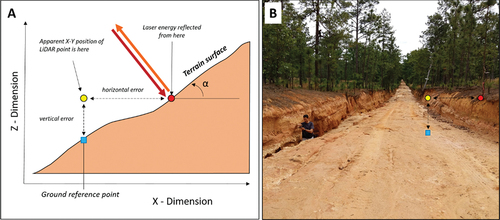
Determining the true changes in elevation differences is also related to the horizontal error in the surfaces. Horizontal error of airborne LiDAR collections today is greater than vertical errors but is typically noted as below 100 cm (with lower horizontal errors with lower flying altitudes). Assessing horizontal error is very challenging. In practice, users of LiDAR data assume that the errors are negligible. The impact of horizontal error in LiDAR data is greater on steeper slopes than low slopes (Hodgson and Bresnahan 2004). In fact, for very low slopes, horizontal error has no affect on vertical error. However, for very steep slopes, such as road cuts or gulleys, the horizontal error is typically noticeable and has implications for volume estimates (Figure 2A-2B). It should also be noted that elevation errors can also result from the surface materials and incidence angles within each LiDAR footprint. Classical remote sensing research with single imagery registered one image to another to minimize the effect of horizontal error (Singh 1989). However, since LiDAR data are collected by a scanner in a moving aircraft, the horizontal and vertical error may vary spatially, as the estimated GNSS-derived position of the sensor position/pointing direction varies with the satellites observed and such satellites are constantly moving. Such variation is known to vary by flight line as the LiDAR pulses within a flight line are collected at a very similar time (within minutes of each other), while the differences in time between flight lines are much greater. As stated earlier, this fact is largely unrecognized by the user community.

Figure 2. A) Impacts on user’s computation of false erosion or deposition caused by horizontal error in LiDAR-derived DEMs, B) the concept applied on the field..

2.5 Spatial variation of horizontal and vertical error

To adequately model elevation change uncertainty, a complete understanding of the sources of error and their relative independence must be understood. For example, in large area change analysis, where multiple flight lines of LiDAR data are used, the spatial variation in elevation error for a single DEM can result from errors in the data collection process – IMU, GNNS baselines, GNNS constellations, atmospheric turbulence, etc. Such causal factors may be well understood, measured, and modeled (e.g. GNNS baselines), while others are well understood but not measured (e.g. atmospheric turbulence). For most scientists using airborne LiDAR data, the process for georegistration and calibration is simply unknown and the scientist simply discounts these possible sources of error. As will be demonstrated in this research, the spatial variation by flight line in vertical error has a profound, but measurable, impact on mapped elevation changes.

It is also well known in the remote sensing community the influence of vegetation and other land covers may affect return density from the ground and thus, a sparser set of ground points to construct a DEM. Lower density of observations on the ground typically results in less accurate DEMs. This has been so well known that FEMA and USGS stated guidelines of accuracy expectations include different requirements based on land cover categories (Heidemann 2018; USGS 2022).

Attempts to estimate and subsequently minimize horizontal errors include horizontal bias estimation and an iterative striping reduction method (Schaffrath, Belmont, and Wheaton 2015). Schaffrath, Belmont, and Wheaton (2015) referred to the differences they observed as “vertical bias attributed to different geoid models” and “poor coregistration of the flight lines.” Differences between geoidal models can be resolved deterministically. The flight line “coregistration” issues are most likely from the varying GNSS observations noted above. In attempting to identify a systematic shift in horizontal error, Schaffrath, Belmont, and Wheaton (2015) estimated shifts ranging from 0.4 m to 5.0 m but were effectively random across the study area. Attempts to resolve horizontal errors include local spatial correlation approaches using both slope and elevation (Besl and McKay 1992; Streutker, Glenn, and Shrestha 2011). The success of these approaches is dependent on the point density and how correlated the displacements are over larger areas. Using an iterative method of trial-error, Schaffrath, Belmont, and Wheaton (2015) examined elevation differences in randomly generated points from different correction surfaces.

Other research that include spatial variation in errors includes stratification into wet/dry areas (Lane, Westaway, and Murray Hicks 2003). Spatially explicit approaches used are correlation of vertical/horizontal LiDAR errors on sloping surfaces (Hodgson and Bresnahan 2004; Schaffrath, Belmont, and Wheaton 2015) or estimates of spatial autocorrelation (Wheaton et al., 2010).

3. Methodology

3.1 LiDAR data collection and processing

The MTC is quite large and problematic to cover quickly in a field reconnaissance, while active restoration and ongoing training takes place. Fortunately, the Army National Guard had previously collected airborne LiDAR data over the entire training base and all of Fort Jackson. In this study of a significant rainfall event, pre-event LiDAR data were collected on 17 December 2014 for the Army between 8:54 am and 11:07 am EST using a LiDAR sensor flown at ~ 1460-m (4800’) altitude. LiDAR collection and processing approaches were not strictly based on the United States Geological Survey (USGS) LiDAR specifications; however, the vendor used quality tests that were “analogous to the spatial distribution and void test as defined by the US Geological Survey (USGS) LiDAR Base Specification Version 1.0” (Quantum Spatial 2015). Scan angles were between ±22 degrees for the 19 flight lines of data collected over the MTC. The flight lines were oriented east-west for the collections. Overlap in flight lines varied from 20% to 50%. Up to five returns per pulse were recorded. In order to post-process the LiDAR data to meet task order specifications, the aeroservice contractor (Quantum Spatial) established 30 ground control points throughout the Fort Jackson, SC project area that were used to validate the LIDAR data. Both natural color and color-infrared imagery were also collected on 17 December 2014. The horizontal projection/datum was Universal Transverse Mercator Zone 17, NAD83 (2011), meters and vertical datum of NAVD1988 (GEOID12A), meters.

The LIDAR data were processed using automatic point classification routines with proprietary software. Subsequent review of the labeled returns was performed by experienced LiDAR analysts using localized automatic classification, manual editing, and peer-based quality control checks. Full dataset point density was an average of 3.2 points per m². After return labeling, the ground return density was an average of 0.93 points per m². We obtained the 2014 point-cloud data as tiles (not in organized flight line files), and unfortunately, LAS points did not include flight line numbers. Because of this limitation in flight line coding, we were unable to evaluate possible flight line-induced biases in the 2014 data.

Reference data for validation was collected by the aeroservice provider using GNNS and OPUS post-processing. Horizontal accuracy estimates by the contractor using building rooflines suggested horizontal errors of 10.4 to 18.0 cm RMSE for all flight lines with maximum errors of 94 cm. Vertical accuracy by the contractor using 30 check-points in open terrain and from non-overlapping data was reported as only .0215 cm (0.072 feet) RMSE or 4.3 cm (0.141 feet) Accuracy_z at the 95% confidence interval.

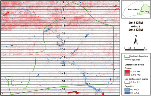
Post-event LiDAR data were collected by the United States Army Corps of Engineers (USACOE) Army Geospatial Center on November 14, 15, 20 and 21 of 2015 using an ALTM_10SEN273 sensor. Fifty-two flight lines, also oriented in the east–west direction, covered the MTC (Figure 3). There was a very small amount of rainfall on November 18 and 19; thus, no LiDAR collection occurred on these days. Concurrent natural color aerial imagery was also collected and provided in a mosaic. The 2015 data were developed based on a horizontal projection/datum of Universal Transverse Mercator Zone 17, NAD83 and vertical datum of EGM2008, both in meters. The Earth Gravitational Model (EGM), such as the EGM2008, was developed by the National Geospatial Intelligence Agency (NGA) as a global vertical datum model. The difference between the Earth Gravitational Model (EGM) for 2008 and NAVD88 for this area of South Carolina is considered negligible (less than 1 cm).

Figure 3. Numeric order of flightlines in the 2015 post-event collection mission shown geographically over the MTC.

Pre- and post-bare earth DEMs were created from the LiDAR data using first a TIN-based data model with all ground labeled LiDAR returns, and second, a linear-interpolation method for converting each TIN to a 1 × 1-m DEM. It has long been recognized that the accuracy of DEMs created from point observations is sensitive to the spatial interpolation method used and, in particular, to the terrain complexity and density of observations (Guo et al., 2010; Hodgson and Bresnahan 2004; MacEachren and Davidson 1987). Others have noted that differences in terrain models produced by different interpolation methods are negligible if the data density is high (Chaplot et al., 2006). The bare earth point density was 0.93 points per m² and 1.5 points per m² for the pre- and post-event DEMs, respectively, which is considered high for deriving a 1 × 1-m DEM. The terrain in our study area is of low to moderate slopes.

3.2 Systematic flight line biases

Assuming the LiDAR sensor unit has been properly boresighted, observed elevation differences between the two DEMs of the same unchanged surface area are typically associated with the GNSS observational differences within/along a flight line. Again, the explanation is that the positional fixes (and errors) are highly correlated in time (i.e. during a flight line) and will typically be somewhat different than the adjacent flight line owing to the time for the aircraft to complete the flight line, reverse direction and begin another flight line. Thus, the positional errors within a flight line are more similar than the errors between flight lines. Still, because of the correlation of GNSS errors in time, the adjacent flight lines will exhibit similar differences than non-adjacent flight lines; thus, there will be greater spatial correlation in errors within a flightline than between flightlines. The spatial errors can be in the horizontal dimension, elevation, or both, although the largest differences are typically in the elevation. Occasionally, when post-processing the LiDAR data, the vendor or contractor may require a re-flight for one or more flight lines, and thus, these flight lines may be collected at a considerably different time than nearby flight lines.

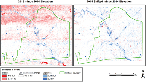
In this study, systematic elevational biases may compromise the change detection analysis as we were looking for surface changes less than 1.0 m. Conducting an initial subtraction of the post-event DEM with the pre-event DEM revealed obvious elevational biases oriented in the east–west direction – consistent with the flight paths (Figure 3). These obvious elevational biases may have resulted from error in the 2014 or 2015 data, or both. A robust and highly precise approach would involve establishing validation data within each flight line to determine a systematic vertical bias from an established and more accurate datum. This strip adjustment approach would also allow for the inclusion of other ancillary data. For the nineteen 2014 flight lines and fifty-one 2015 flight lines, this level of effort would be substantial, such as collecting ten or more ground reference points per flight line. Moreover, we did not have access to 2014 LiDAR point clouds with flight line codes (they may no longer exist). The ground reference problem is exacerbated as most of the landscape is covered by forests, requiring total-station-based survey methods, as survey grade GNNS would not be possible under the canopy.

We offer an alternative approach (approach two we suggested under section 2.2 Normalizing the Surface) using one LiDAR-derived surface as the control datum and identifying and removing systematic differences in the second LiDAR-derived surface. This second approach requires no ground reference data specifically but does require the analyst to select comparison boundaries in areas known to have stable surfaces between the two collection dates. Numerous (11) field visits, with the initial broad scale visit on 25 February 2016, along sand roads and cross-country through the forests probing possible surface change areas and apparent false changes allowed us to select reliable “no-change boundaries”. Our final visits in May 2017 were to conduct many cross-country walks to clarify possible sand movement anomalies. We choose to use the pre-event DEM (2014) as the control as it was collected/processed/validated under a more normal contracting mechanism with appropriate quality control. As noted earlier, the post-event LiDAR collection was a quick response to a disaster event and did not follow typical contracting and QA/QC controls. Of note, this problem context is very typical of disaster response using remote sensing with LiDAR or other imagery. In this study, all elevations in a 20-m-wide buffer around a transect running across all 51 flightlines, over a portion of the MTC for which virtually little erosion/deposition was observed, were used for the strip-adjustment calibration. Both field verification and visual interpretation of the coincident aerial imagery were utilized to verify. Average elevation differences from the 2014 DEM for each flight line were computed (Figure 4). Almost all 2015 (i.e. the post-event collection) flight lines indicated an under-prediction in elevation (as compared to the 2014 DEM as a control surface) with an increasing under-prediction for the northern flight lines. The average difference was −9.6 cm. Since the 2015 LiDAR data were originally processed by the vendor in a rapid manner for the disaster recovery effort, the assumption is the effort in processing the post-event data was less than the 2014 pre-event data, and presumably less accurate with biases. Thus, the 2014 data were regarded as the control surface (i.e. the more correct surface) and the average difference applied as elevation shifts to all LiDAR elevations within each of the 2015 flight lines. After all shifts were completed, a new 2015 DEM was created and subsequently, a new elevation difference surface computed (Figure 5). Using the 20-m-wide buffer corridor around our established transect as the control area (i.e. the area where no surface change would have occurred), we noted that the average difference in elevations between the 2014 and 2015 DEMs was now only −1.7 cm, indicating a very slight overall negative difference in elevation for the shifted 2015 data.

Figure 4. Average elevation differences (in cm) between all locations in a 20 m buffered north-south transect across the MTC.

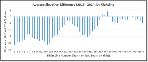
Figure 5. Mapped elevation differences (in cm) between 2014 and 2015 DEMs (a). Elevation differences after flight line bias analysis and compensation in (b).

3.3 Reference data for LiDAR validation and topographic change

Field observation data were in the form of 1) high accuracy elevation data from GNSS and Total Station surveys and 2) manual borehole and pits. We collected high accuracy (~2.5 cm at the 95% level) elevation observations (n = 42) over areas of observed sediment flux and areas of no-change (n = 237). Sites for collecting field observations were guided by the MTC conservation manager (also a coauthor of the manuscript). Field data were collected between 25 February 2016 (4 months after the event) and 8 May 2017 (within 15 months after the event). An initial visit to all candidate borehole locations was conducted on 25 February 2016, guided by the on-site conservation manager. The conservation manager confirmed, in the field with us, the candidate locations for boreholes did not change in morphology. The open-canopy field observation positions were collected using a Topcon GRS-1 RTK receiver with 5 seconds or more occupations using the Real-Time Network in South Carolina (SCRTN). Performance tests of the SCRTN network by the South Carolina Geodetic Survey found accuracies (X-Y-Z) of approximately 2.5 cm at the 95% confidence level. Only FIX observations (referring to the integer wave positioning) were collected, averaged, and used to validate the LiDAR-derived DEMs. Eleven other GNSS observations with a FLOAT solution were used only to locate an auger hole or pit in moderate canopy situations. Subsequent evaluation of the observed data found a few (3) observations with VDOP or PDOP values greater than 4.0. Only observations with VDOP/PDOP values less than 4.0 were used for the DEM validation.

Observations (n = 33) under forest canopy at Bee Branch (Figure 1) were collected using a Sokkia Set 530 R total station from GNSS/OPUS-derived monument positions. Three monuments were established in open canopy conditions using 3-hour observations with a static GNNS XR90 collecting at 15-second intervals. Subsequent post-processing of the observations using OPUS rapid static provided positions of the inserted monument estimated accuracies of 2 cm and 3 cm RMSE horizontal and vertical accuracies, respectively. These two monuments were used for the total station control (base and back-sight). A third monument was established using the GRS-1 and SCRTN to provide a check in the total station-derived measurements. Field data on sediment flows and no-change surfaces under forest canopy were collected with the total station. All observations were made at a distance of less than 60 m from the total station.

Manual boreholes or open pits (n = 27) were made in both the open-canopy and closed-canopy conditions over sediment flows as validation for the LiDAR-derived change detection using a custom Italian auger (courtesy of Bruno Piovan). The boreholes in the Free Maneuver Area and Bee Branch were conducted together with field investigation to validate the accuracy of the LiDAR data. These validations occurred between February 2016 and May 2017 so less than 1 year after the flood. In Lundy’s Lane, the field investigations were conducted in May 2017. No reconstruction activities were performed by the military staff in these periods of time at these locations, and we found no visible evidence that other events in this one- and one-half year field campaign caused changes in the deposits we investigated.

3.4 Field investigation to calibrate for true/false changes

Eleven field campaigns were conducted to verify locations where no topographic changes occurred, to identify/quantify depth of changes for other areas and to revisit numerous other locations to verify anomalies and causal agents for the sand change. To evaluate the absolute accuracy of each of the two DEMs, a set of reference points where no change in land cover had occurred (n = 230) since the first LiDAR collection in 2014. An additional set of reference points (n = 49) where surface elevation changes had occurred was collected to supplement the 230 reference points in the validation of the 2015 DEM. Locations were identified during site visits and positions determined in the field with RTK GNSS and total station methods. The location of each reference point was measured with the Topcon GNSS receiver in RTK mode. The elevation for each reference point was extracted from the 2014 and 2015 (after vertical shifts) DEMs and compared to the reference elevations.

4. Results

4.1 Validation

Mean signed error for the 2014 and 2015 DEMs was −3.9 cm and −3.62 cm, respectively (Table 1). Thus, a small under-prediction in elevations of about 4 cm was observed for the entire MTC. Statistical expressions of the 2014 and 2015 DEMs were 7.8 cm and 8.3 cm RMSE, respectively.

Table 1. Error (in cm) for pre- and post-flood event DEMs based on field data.

Statistic	2014	2015
Number of observations	230	279
Largest Negative Error	-35.27	-30.83
Largest Positive Error	18.46	25.05
Mean Error	-3.93	-3.62
RMSE (68% confidence)	7.81	8.32
Accuracyz (95% confidence)	15.31	16.30

Transformation to a 95% confidence threshold was 15.3 and 16.3 cm, respectively. Interpretation of the customary error statistics should be used with consideration of the degree of non-normality of the error distribution. Elevation errors for both 2014 and 2015 were not normal (Jacque-Bera test, p = 0.000) and somewhat skewed. Skewness and kurtosis for the 2014 DEM errors were −0.4675 and 2.7131, respectively. Skewness and kurtosis for the 2015 DEM errors were −0.5077 and 1.7576, respectively. Thus, Equation 1(1) $\mathrm{R}\mathrm{M}\mathrm{S}{\mathrm{E}}_{\mathrm{d}\mathrm{i}\mathrm{f}\mathrm{f}}(68\mathrm{\%})=\mathrm{s}\mathrm{q}\mathrm{r}\mathrm{t}(\mathrm{R}\mathrm{M}\mathrm{S}{{\mathrm{E}}_{\mathrm{D}\mathrm{E}\mathrm{M}-1}}^2+\mathrm{R}\mathrm{M}\mathrm{S}{{\mathrm{E}}_{\mathrm{D}\mathrm{E}\mathrm{M}-2}}^2)$(1) is used as a guide for establishing confidence thresholds with the knowledge that the normality assumption underlying equation 1(1) $\mathrm{R}\mathrm{M}\mathrm{S}{\mathrm{E}}_{\mathrm{d}\mathrm{i}\mathrm{f}\mathrm{f}}(68\mathrm{\%})=\mathrm{s}\mathrm{q}\mathrm{r}\mathrm{t}(\mathrm{R}\mathrm{M}\mathrm{S}{{\mathrm{E}}_{\mathrm{D}\mathrm{E}\mathrm{M}-1}}^2+\mathrm{R}\mathrm{M}\mathrm{S}{{\mathrm{E}}_{\mathrm{D}\mathrm{E}\mathrm{M}-2}}^2)$(1) was violated.

A 95% confidence threshold of 22.8 cm was derived from the accuracy of the two dates of DEMs using equations (1)(1) $\mathrm{R}\mathrm{M}\mathrm{S}{\mathrm{E}}_{\mathrm{d}\mathrm{i}\mathrm{f}\mathrm{f}}(68\mathrm{\%})=\mathrm{s}\mathrm{q}\mathrm{r}\mathrm{t}(\mathrm{R}\mathrm{M}\mathrm{S}{{\mathrm{E}}_{\mathrm{D}\mathrm{E}\mathrm{M}-1}}^2+\mathrm{R}\mathrm{M}\mathrm{S}{{\mathrm{E}}_{\mathrm{D}\mathrm{E}\mathrm{M}-2}}^2)$(1) and (2(2) $\mathrm{A}\mathrm{c}\mathrm{c}\mathrm{u}\mathrm{r}\mathrm{a}\mathrm{c}{\mathrm{y}}_{\mathrm{d}\mathrm{i}\mathrm{f}\mathrm{f}}(95\mathrm{\%})=\mathrm{R}\mathrm{M}\mathrm{S}{\mathrm{E}}_{\mathrm{d}\mathrm{i}\mathrm{f}\mathrm{f}}\ast 1.96$(2) ). When using the 22.8 cm threshold to screen the validation points (230) where no elevation change occurred between 2014 and 2015 only one point (−27.1 cm elevation error) would be incorrectly classified as an elevation change. Similarly, applying the same threshold to check the change/no-change accuracy of locations (n = 27) where we field-measured sand deposition, only five points would be incorrectly listed as no-change.

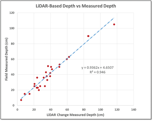
Elevation changes at the location of 27 auger holes/pits were compared to measure the depth of sand deposition. The range of errors was from an under-prediction of −14.1 to an over-prediction of +11.5 cm, with an average error of −2.11 cm, indicating a slight bias in under-predicting sand depths. Sands were probably water-saturated in the first days following the event, and their drainage in the subsequent time may have led to partial collapse of the pore due to lowering hydrostatic pressure (“ripening” process). Thus, the sediment may have loose volume, leading to lowering of the topographic surface. A regression analysis showed a high degree of correlation (R² of 0.946) between LiDAR-derived sediment depths and field measured depths (Figure 6).

Figure 6. Observed versus LiDAR-based measurements for 27 sand holes/pits. All values in centimetres.

Landscape elevation changes were again mapped for the entire MTC using the 22.8 cm threshold to screen for elevation differences greater than our level of detection. We regarded any difference greater than 22.8 cm to have a high confidence this difference observed with the LiDAR-based approach to be an actual elevational change. Subsequently, we refer to elevation differences of greater than 22.8 cm to be “real” changes. As the area of changes greater than 22.8 cm is relatively small in comparison to the area of the study environment, only dense areas of change that are particularly notable as anomaly examples are shown. Anomalies are places where elevation differences are greater than the 22.8 cm detection limit but are, in fact, not actual elevation changes – the differences in observed elevations are due to other elevation modeling factors. In each case, the nature of the change – false or real (as verified by field observation) – erosion/deposition is presented and discussed.

4.2 Anomalies

The Davis Pond area (Figure 1) is a good example of false changes (Figure 7A) emanating from changes in LiDAR ground return distributions – not actual elevation changes observed in the LiDAR data. Airborne LiDAR systems typically operate with an infrared laser (e.g. 905 µm or 1550 µm) and water absorbs the laser pulse resulting in no LiDAR return. If the water is turbulent or has floating material, then some laser pulses are returned. The Davis Pond case provides an example of both issues. As noted from the pre- and post-event aerial optical imagery flown concurrently with the LiDAR collection missions, the water level in Davis Pond was higher in the post-event LiDAR collections (Figure 8). Thus, ground returns near the water line in the 2014 collection are absent in the post-event 2015 collection. Thus, the interpolation routines (TIN in this study) extrapolate “level” surfaces across the pond to suggest an elevated surface in the 2015 data (Figure 7B). However, the area near the dam contained considerable material on the water surface and a notable depositional area on the southeastern corner of the dam (Figure 9).

Figure 7. Davis pond exhibiting considerable increase in elevation and decrease in elevation (in m) near dam on left and explanation of false deposition caused by missing LiDAR returns over water.

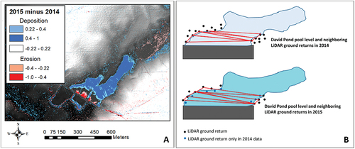
Figure 8. Natural color imagery of Davis Pond during 2014 LiDAR collection (A) and 2015 LiDAR collection (B) showing changes in pool level.

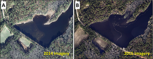
Figure 9. Sand deposition (two small lacustrine deltas) on southeast corner of Davis Pond.

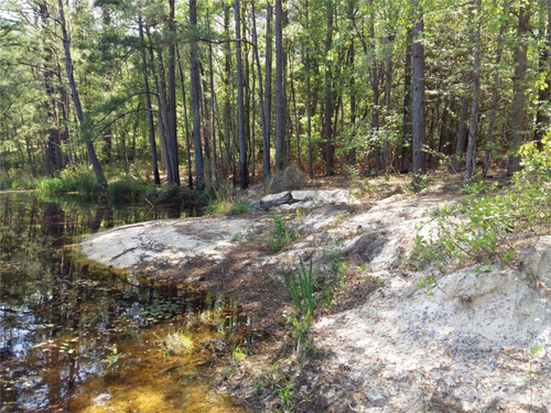
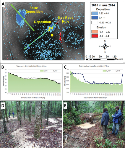
The erosional and depositional area at the Bee Branch (Figure 1) crossing contained the deepest sediment deposition – over 117 cm in depth for a large area (Figure 10). Sand was eroded off a downhill road and through an overturned tree, displacing the tree and creating a very deep erosional remnant. The sand then moved into the Bee Branch flood plain and ponded quickly because of the water present during the rainfall event. Four auger hole measurements were placed in the deep sand deposition and compared to the LiDAR estimates of deposition. Auger measured depths of 105, 90, 90, and 50 cm corresponded to LiDAR-derived changes of 117, 87, 85, and 41 cm, respectively. Just uphill to the west, the LiDAR DoD indicated an apparent equally large depositional area. However, field visits indicated no sand deposition. An evaluation with the concurrent imagery sources indicated that this was also a false depositional area where water had collected during the post-event LiDAR acquisition and, similar to Davis Pond context, resulted in a false increase because of the absence of LiDAR returns.

Figure 10. Profiles across false deposition and actual depositions and location of validation points in yellow (A), transect across false deposition (B), transect across deposition piles (C), deposition area up to 1.17 m in thickness (D), and actual erosion (i.e. tree root hole) (E) in Bee Branch area.

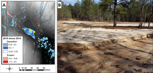
The Free Maneuver Area (formerly called the Dudded Area), on the eastern side of MTC (Figure 1) was a former practice environment for munitions testing (Figures 11). Prior to the Army’s use of the landscape the area was under agricultural production with noticeable terraces shown in the LiDAR DEMs but not noticeable in the field. A large but somewhat shallow depositional area (25 to 50 cm in depth) was visited in a broad field with a few native pines. The source of the sand in this depositional area was from the road, and likely largely from the eroded sides of the sand roads about 150–200 m away.

Figure 11. A) Lidar change detection model of the Free Maneuver Area (south). Reference points used for validation are shown in yellow with erosion/deposition in m; B) sandy deposition in Free Maneuver Area (south).

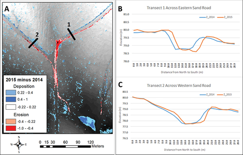
Additionally, the parallel lines of “false” erosion and depositional areas along the sand road north of the Free Maneuver Area are easily seen. Field visits verified that there was some erosion and deposition on the sides of the road, but the horizontal displacement in the two LiDAR collections greatly magnifies the apparent elevation changes (Figure 12). The sand roads are incised in the environment with very steep sides; thus, a horizontal displacement in the LiDAR returns would result in a false erosion or deposition. The 2015 LiDAR data for this flight line are displaced to the southeast of the 2014 LiDAR data. It is unknown which LiDAR dataset (2014 or 2015) is more correct and no reliable ground reference data can be used to resolve the issue. It might be possible to spatially correlate the two surfaces, under the assumption there was no real elevational change to determine an adequate displacement.

Figure 12. A) Location of the two transects (B and C) along the eastern and western sand roads supplying sand to the road feeding the Free Maneuver Area showing horizontal error expressed as a mismatch between profiles.

5. Discussion

The results from comparing mean differences in surface elevations between 2015 and 2014 collections, in a narrow band (20 m) of terrain (along a transect crossing all flightlines) that did not change between dates, indicate clear flight line biases. The elevation differences by flight line also indicate trends from one flight line to the next, strongly suggesting a causal factor of the quality of the GNSS observations.

As a note, the remaining discrepancies in elevations between collection dates include any systematic flight line bias from the 2014 collection. The 2014 collection likely contained somewhat similar, but expectedly lower, biases from the same causal factors as the level-of-effort for post-processing the data by the vendor were more substantial. As stated earlier, we did not have the point-cloud data partitioned into the original flight lines and thus, could not evaluate the possible biases in the 2014 data.

Correcting the elevation biases in the 2015 data using the 2014 data as the control surface is adequate for change-detection studies where only the pre-post LiDAR data are analyzed. If other ancillary data are also needed, such as flora or fauna surveys, for subsequent geospatial analysis with the topographic change surfaces then normalizing both the 2014 and 2015 data to a standard known datum using ground reference points is ideal. In other words, rather than using the 2014 topographic surface as the “control” a better approach would be to transform both the 2014 and 2015 DEMs to a surface with a higher confidence in elevations. Unfortunately, the number of ground reference points for normalizing all of the flight lines for two separate dates of collection is substantial and would be problematic to collect for an active military training base.

Several false change anomalies related to the impacts of water were noted in this research. Since airborne LiDAR almost always uses a near-infrared wavelength sensor, the result is an absence of a LiDAR return in areas of standing water. These absence of returns result in not only lower density of observations but spatially correlated absences around and within water bodies; thus, the resulting TIN and/or DEM is compromised around these features. These anomalies are unusual products but systemic of a large-scale rainfall event and will likely be present in other research efforts using airborne LiDAR for change detection work. These issues strongly suggest coincident or near coincident imagery (e.g. natural color or false-color) with a LiDAR collection and, ideally, field observations at places where these anomalies may occur.

6. Conclusions

The use of manned airborne LiDAR for mapping erosion and sediment deposition at levels of over 22 cm change is possible with LiDAR collections as noted in this research. Conducting a change analysis from such airborne data, however, is highly dependent on the collection parameters that result in an accurate set of “ground” returns. These parameters are largely dependent on the flying altitude and LiDAR pulse rate that produce a dense set of LiDAR returns to begin stratifying for ground and non-ground. From our analysis of the LiDAR datasets, we found a vertical bias in the LiDAR data collected after the 2015 storm event. The bias varied by flight line and obviously correlated with the gradually changing GNSS constellations over time that are used for the onboard GNSS positional determinations. The adjustments that we made largely obviated the bias.

As noted earlier, other strip adjustment methods exist, many of which are more rigorous but require additional collection data/parameters but may be more appropriate for different study environments. Additionally, since version 1.1 of the USGS guidelines, accuracy requirements for within and between strips/flightlines (referred to as overlap in flight swaths in the USGS terminology) for each quality level have been defined (USGS 2022). The LiDAR collections/processing methods available from the U.S. Army did not follow the USGS LiDAR base specification guidelines specifically for QL0 through QL3 data. In concept, following and meeting such guidelines would provide empirical evidence of the need (or not) to perform subsequent strip adjustments depending on the detection limits desired. These guidelines require the assessment and reporting of consistency in elevations (reported as root mean squared difference) created from observations in different flightlines. For example, a QL1 dataset would require differences of less than 8 cm. However, and this is critical to note, the specifications in the USGS guidelines specify that consistency assessments use observations “in nonvegetated areas of only single returns and with slopes of less than 10 degrees.” For our study environment, most of the areas of mapped change has a vegetation overstory and some with slopes greater than 10 degrees. Thus, the consistency assessment following USGS guidelines would not be representative of appropriate thresholds. The second issue that must be considered for future applications is the ponding of water on the landscape, the resulting missing LiDAR returns in the wet areas, and the interpretation of these areas as false depositional areas.

Airborne LiDAR data, with appropriate care and processing, are a useful broad area mapping method for topographic change – even for small changes (e.g. 22 cm) in topography. With these pre- and post-airborne LiDAR collections, the ability to predict sand deposition (an elevation increase) could be performed with an average absolute error of 4.7 cm. In this study, we found the sources of erosional material from the 2015 rainfall event were almost exclusively associated with material from the sand roads or side of roads, often sharply cut through the terrain.

Acknowledgments

We express our appreciation to Chris Robbins at the South Carolina Army National Guard (SCARNG) and William Poulson and James Hibbert at the University of South Carolina. Special appreciation to Bruno Piovan who designed and crafted a custom sand auger, with an enclosed sleeve, for the stratigraphic field work.

Disclosure statement

No potential conflict of interest was reported by the authors.

Data availability statement

The final DEMs, both pre and post- event, with the supporting ancillary data are available at: https://osf.io/7axbw/?view_only=e3fcb252d0d24761ba3f86eebb8f6543. https://osf.io/7axbw/?view_only=e3fcb252d0d24761ba3f86eebb8f6543.

The field data that support the findings of this study are available from the corresponding author, upon reasonable request. Requests for the airborne LiDAR point cloud must be made to the South Carolina Army National Guard.

Additional information

Funding

This research was carried out with the support of the University of South Carolina contract to SCARNG (#21600-FC56) This article has been published with funds provided by the PRIN project ”SYLVA”, (Prot. 20177H5KLM). 

Notes

1. We note the use of the terms digital elevation model (DEM) and digital terrain model (DTM) for describing a regular spaced raster of the bare-earth terrain surface in both the practice and literature. We use the acronym DEM exclusively, following USGS and the preponderance of literature.

References

- Anderson, S. W. 2019. ”Uncertainty in Quantitative Analyses of Topographic Change: Error Propagation and the Role of Thresholding.” Earth Surface Processes and Landforms 44 (5): 1015–21.
- Besl, P. J., and H. D. McKay. 1992. “A Method for Registration of 3-D Shapes.” IEEE Transactions on Pattern Analysis & Machine Intelligence 14 (2): 239–256. https://doi.org/10.1109/34.121791.
- Brasington, J., J. Langham, and B. Rumsby. 2003. “Methodological Sensitivity of Morphometric Estimates of Coarse Fluvial Sediment Transport.” Geomorphology 53 (3–4): 299–316. https://doi.org/10.1016/S0169-555X(02)00320-3.
- Cavalli, M., B. Goldin, F. Comiti, F. Brardinoni, and L. Marchi. 2017. “Assessment of Erosion and Deposition in Steep Mountain Basins by Differencing Sequential Digital Terrain Models.” Geomorphology 291:4–16. https://doi.org/10.1016/j.geomorph.2016.04.009.
- Challis, K., C. Carey, M. Kincey, and A. J. Howard. 2011. “Assessing the Preservation Potential of Temperate, Lowland Alluvial Sediment Using Airborne LiDar Intensity.” Journal of Archaeological Science 38 (2): 301–311. https://doi.org/10.1016/j.jas.2010.09.006.
- Chaplot, V., F. Darboux, H. Bourennane, S. Leguédois, N. Silvera, and K. Phachomphon. 2006. “Accuracy of Interpolation Techniques for the Derivation of Digital Elevation Models in Relation to Landform Types and Data Density.” Geomorphology 77 (1–2): 126–141. https://doi.org/10.1016/j.geomorph.2005.12.010.
- Chen, Z., J. Li, and B. Yang. 2021. “A Strip Adjustment Method of UAV-Borne LiDar Point Cloud Based on DEM Features for Mountainous Area.” Sensors 21 (8): 2782. https://doi.org/10.3390/s21082782.
- Croke, J., P. Todd, C. Thompson, F. Watson, R. Denham, and G. Khanal. 2013. “The Use of Multi-Temporal LiDar to Assess Basin-Scale Erosion and Deposition Following the Catastrophic January 2011 Lockyer Flood, SE Queensland, Australia.” Geomorphology 184:111–126. https://doi.org/10.1016/j.geomorph.2012.11.023.
- Eagleston, H., and J. L. Marion. 2020. “Application of Airborne LiDar and GIS in Modeling Trail Erosion Along the Appalachian Trail in New Hampshire, USA.” Landscape and Urban Planning 198:103765. https://doi.org/10.1016/j.landurbplan.2020.103765.
- Favalli, M., A. Fornaciai, and M. T. Pareschi. 2009. “LIDAR Strip Adjustment: Application to Volcanic Areas.” Geomorphology 111 (3–4): 123–135. https://doi.org/10.1016/j.geomorph.2009.04.010.
- Fekry, R., W. Yao, L. Cao, and X. Shen. 2021. “Marker-Less UAV-Lidar Strip Alignment in Plantation Forests Based on Topological Persistence Analysis of Clustered Canopy Cover.” ISPRS International Journal of Geo-Information 10 (5): 284. https://doi.org/10.3390/ijgi10050284.
- Glira, P., N. Pfeifer, C. Briese, and C. Ressi. 2015. “Rigorous Strip Adjustment of Airborne Laserscanning Data Based on the ICP Algorithm.” ISPRS Annals of the Photogrammetry, Remote Sensing & Spatial Information Sciences II-3W (5): 73–80. https://doi.org/10.5194/isprsannals-II-3-W5-73-2015.
- Grove, J. R., J. Croke, and C. Thompson. 2013. “Quantifying Different Riverbank Erosion Processes During an Extreme Flood Event.” Earth Surface Processes and Landforms 38:1393–1406. https://doi.org/10.1002/esp.3386.
- Guo, Q., W. Li, H. Yu, and O. Alvarez. 2010. “Effects of Topographic Variability and Lidar Sampling Density on Several DEM Interpolation Methods.” Photogrammetric Engineering and Remote Sensing 76 (6): 701–712. https://doi.org/10.14358/PERS.76.6.701.
- Heidemann, H. K. 2018. Lidar Base Specification (Ver. 1.3, February 2018): U.S. Geological Survey Techniques and Methods, Book 11, Chap. B4, 101 P. US Geological Survey. https://doi.org/10.3133/tm11b4.
- Hodgson, M. E., and P. Bresnahan. 2004. “Accuracy of Airborne Lidar-Derived Elevation: Empirical Assessment and Error Budget.” Photogrammetric Engineering & Remote Sensing 70 (3): 331–339. https://doi.org/10.14358/PERS.70.3.331.
- Hodgson, M. E., and G. Morgan. 2021. “Modeling Sensitivity of Topographic Change with sUAS Imagery.” Geomorphology 375 (15): 107563. https://doi.org/10.1016/j.geomorph.2020.107563.
- James, L. A., M. E. Hodgson, S. Ghoshal, and M. M. Latiolais. 2012. “Geomorphic Change Detection Using Historic Maps and DEM Differencing: The Temporal Dimension of Geospatial Analysis.” Geomorphology 137 (1): 181–198. https://doi.org/10.1016/j.geomorph.2010.10.039.
- Kim, M.-K., H.-G. Sohn, and S. Kim. 2020. “Incorporating the Effect of ALS-Derived DEM Uncertainty for Quantifying Changes Due to the Landslide in 2011, Mt. Umyeon, Seoul.” GIScience and Remote Sensing 57 (3): 287–301. https://doi.org/10.1080/15481603.2019.1687133.
- Lane, S. N., R. M. Westaway, and D. Murray Hicks. 2003. “Estimation of Erosion and Deposition Volumes in a Large, Gravel-Bed, Braided River Using Synoptic Remote Sensing.” Earth Surface Processes and Landforms 28 (3): 249–271. https://doi.org/10.1002/esp.483.
- MacEachren, A. M., and J. V. Davidson. 1987. “Sampling and Isometric Mapping of Continuous Geographic Surfaces.” The American Cartographer 14 (4): 299–320. https://doi.org/10.1559/152304087783875723.
- Maling, D. H. 1989. Measurement of Area. New York: Elsevier. https://doi.org/10.1016/B978-0-08-030290-4.50010-4.
- Milan, D. J., G. L. Heritage, A. R. Large, and I. C. Fuller. 2011. “Filtering Spatial Error from DEMs: Implications for Morphological Change Estimation.” Geomorphology 125 (1): 160–171. https://doi.org/10.1016/j.geomorph.2010.09.012.
- Nourbakhshbeidokhti, S., A. M. Kinoshita, A. Chin, and J. L. Florsheim. 2019. “A Workflow to Estimate Topographic and Volumetric Changes and Errors in Channel Sedimentation After Disturbance.” Remote Sensing 11 (5): 586. https://doi.org/10.3390/rs11050586.
- Nuth, C., and A. Kääb. 2011. “Co-Registration and Bias Corrections of Satellite Elevation Data Sets for Quantifying Glacier Thickness Change.” The Cryosphere 5 (1): 271–290. https://doi.org/10.5194/tc-5-271-2011.
- Pelletier, J. D., and C. A. Orem. 2014. “How Do Sediment Yields from Post-Wildfire Debris-Laden Flows Depend on Terrain Slope, Soil Burn Severity Class, and Drainage Basin Area? Insights from Airborne-LiDar Change Detection.” Earth Surface Processes and Landforms 39 (13): 1822–1832. https://doi.org/10.1002/esp.3570.
- Perroy, R. L., B. Bookhagen, G. P. Asner, and O. A. Chadwick. 2010. “Comparison of Gully Erosion Estimates Using Airborne and Ground-Based LiDar on Santa Cruz Island, California.” Geomorphology 118 (3–4): 288–300. https://doi.org/10.1016/j.geomorph.2010.01.009.
- Quantum Spatial. 2015. Focus on Fort Jackson: LiDAR Q/C and Data Exploitation Report. dated 16 April 2015.
- Rentsch, M., and P. Krzystek. 2012. “Lidar Strip Adjustment with Automatically Reconstructed Roof Shapes.” Photogrammetric Record 27 (139): 272–292. https://doi.org/10.1111/j.1477-9730.2012.00690.x.
- Schaffrath, R., P. Belmont, and J. Wheaton. 2015. “Landscape-Scale Geomorphic Change Detection: Quantifying Spatial Variable Uncertainty and Circumventing Legacy Data Issues.” Geomorphology 250:334–348. https://doi.org/10.1016/j.geomorph.2015.09.020.
- Singh, A. 1989. “Review Article Digital Change Detection Techniques Using Remote Sensing.” International Journal of Remote Sensing 10 (6): 989–1003. https://doi.org/10.1080/01431168908903939.
- Streutker, D. R., N. F. Glenn, and R. Shrestha. 2011. “A Slope-Based Method for Matching Elevation Surfaces.” Photogrammetric Engineering & Remote Sensing 77 (7): 743–750. https://doi.org/10.14358/PERS.77.7.743.
- Toth, C., and D. A. Grejner-Brzezinska 2009. Airborne LiDar Reflective Linear Feature Extraction for Strip Adjustment and Horizontal Accuracy Determination. Ohio Department of Transportation, Report No. FHWA/OH-2008/15. https://rosap.ntl.bts.gov/view/dot/18475.
- Tseng, C. M., C. W. Lin, C. P. Stark, J. K. Liu, L. Y. Fei, and Y. C. Hsieh. 2013. “Application of a Multi‐Temporal, LiDar‐Derived, Digital Terrain Model in a Landslide‐Volume Estimation.” Earth Surface Processes and Landforms 38 (13): 1587–1601. https://doi.org/10.1002/esp.3454.
- USGS. 2022. Lidar Base Specification (Ver. 2022 Rev A, April 2022). https://www.usgs.gov/ngp-standards-and-specifications/lidar-base-specification-online.
- Vaaja, M., J. Hyyppa, A. Kukko, H. Kaartinen, H. Hyyppa, and P. Alho. 2011. “Mapping Topography Changes and Elevation Uncertainty Using a Mobile Laser Scanner.” Remote Sensing 3 (3): 587–600. https://doi.org/10.3390/rs3030587.
- Wheaton, J. M., J. Brasington, S. E. Darby, and D. A. Sear. 2009. “Accounting for Uncertainty in DEMs from Repeat Topographic Surveys: Improved Sediment Budgets.” Earth Surface Processes and Landforms 156:136–156. https://doi.org/10.1002/esp.1886.
- Zhang, Y., X. Xiong, M. Zheng, and X. Huang. 2015. “LiDar Strip Adjustment Using Multifeatures Matched with Aerial Images.” IEEE Transactions on Geoscience and Remote Sensing 53 (2): 976–987. https://doi.org/10.1109/TGRS.2014.2331234.