Water index and Swin Transformer Ensemble (WISTE) for water body extraction from multispectral remote sensing images

ABSTRACT

Automatic surface water body mapping using remote sensing technology is greatly meaningful for studying inland water dynamics at regional to global scales. Convolutional neural networks (CNN) have become an efficient semantic segmentation technique for the interpretation of remote sensing images. However, the receptive field value of a CNN is restricted by the convolutional kernel size because the network only focuses on local features. The Swin Transformer has recently demonstrated its outstanding performance in computer vision tasks, and it could be useful for processing multispectral remote sensing images. In this article, a Water Index and Swin Transformer Ensemble (WISTE) method for automatic water body extraction is proposed. First, a dual-branch encoder architecture is designed for the Swin Transformer, aggregating the global semantic information and pixel neighbor relationships captured by fully convolutional networks (FCN) and multihead self-attention. Second, to prevent the Swin Transformer from ignoring multispectral information, we construct a prediction map ensemble module. The predictions of the Swin Transformer and the Normalized Difference Water Index (NDWI) are combined by a Bayesian averaging strategy. Finally, the experimental results obtained on two distinct datasets demonstrate that the WISTE has advantages over other segmentation methods and achieves the best results. The method proposed in this study can be used for improving regional to continental surface water mapping and related hydrological studies.

KEYWORDS:

• Deep learning
• water body extraction
• Swin Transformer
• water index
• dual-encoder

1. Introduction

Water bodies such as ponds, rivers, lakes, and reservoirs are indispensable components of ecosystems, and they play important roles in hydrological cycles and local climate regulation (Sawaya et al. 2003). Mapping surface water dynamics is of great importance for sustainable development (Pickens et al. 2022). Water body extraction has long been a focus in many disciplines (Sabatini et al. 2022; Xu et al. 2022). For example, the alterations of Arctic rivers can significantly impact ecosystem functions, and mapping such rivers is essential for understanding the uncertainty of future global climate conditions (Li et al. 2022). With the rapid development of earth observation technology, remote sensing images achieve higher resolution and larger spatial coverage than other image types (Feyisa et al. 2014), enabling water body extraction, water resource surveying, flood monitoring, etc (Rokni et al. 2014).

Water body extraction methods mainly include intraspectral relationship, single-band threshold, water body index, object-oriented, and image classification methods (Weng 2012). The single-band threshold method extracts a water body based on the strong absorption characteristics in the mid-infrared and near-infrared bands. The intraspectral relationship method analyses the spectral curve of water between different bands to distinguish between water bodies and the background. Water body index methods mainly include the normalized difference water index (NDWI), which highlights the reflectivity difference between the green band and the near-infrared band and improves the separation between water and nonwater categories (McFeeters 1996). Based on the NDWI, the modified normalized difference water index (MNDWI) replaces the near-infrared band with the shortwave infrared band, reducing the effects of building shadows and soil even further. The enhanced water index (EWI) applies the shortwave infrared (SWIR) band to the NDWI calculation process, enhancing the water extraction effect in semiarid areas. The automatic thresholding method automatically selects segmentation thresholds based on the histogram of an image, reducing the reliance on manual threshold selection (Ovakoglou et al. 2021). An object-oriented method segments the input image into a series of objects according to their spatial features and topological relationships and then extracts water bodies based on the optimal segmentation scale and constructs segmentation rules (Belgiu and Dragut 2016). This kind of method generally performs well, but the segmentation strategy selection process is complicated. Specifically, such methods rely on preprocessing, constructing segmentation rules and postprocessing to obtain good segmentation results. Unsupervised classification methods include K-means, iterative self-organizing data analysis (ISODATA), and cluster analyses, which only perform feature extraction and cluster analysis on remote sensing images and classify clusters based on statistical feature differences. Supervised classification approaches, such as decision tree (DT), formulates classification rules based on spatial data and knowledge mining (Song et al. 2020). Aiming at finding an optimal hyperplane, a support vector machine (SVM) separates water samples from other samples in the feature space (Huang et al. 2018; Koda et al. 2018).

With the continuous development of deep learning theory in recent years, deep learning methods have become increasingly prevalent in remote sensing image interpretation tasks, especially water body extraction (Lu et al. 2022; An and Rui 2022; Yu et al. 2017; Zhang et al. 2021). Miao et al. (2018) designed a restricted receptive field deconvolution network (RRF DeconvNet) for water segmentation, training segmentation networks with an edge weighting loss and testing the performance of their method on Google Earth images. Li et al. (2019) adopted fully convolutional networks to extract water areas using very-high-resolution (VHR) images when the dataset scale was inadequate. Although the abovementioned methods have achieved relatively good results, these models can use only local information instead of global semantic information (Sun et al. 2022).

Recently, Transformer has achieved impressive performance in multiple domains, across multiple datasets and in a variety of tasks. Vaswani et al. (2017) first proposed the Transformer model and used it in natural language processing tasks. In contrast with CNN-based models, the Transformer network structure incorporates an attention mechanism (Bahdanau, Cho, and Bengio 2014), employing an encoder-decoder network structure as opposed to a sequential structure to capture global features. The Vision Transformer’s (ViT) success provides further evidence of the application potential of Transformer in dense prediction tasks such as image classification and semantic segmentation in the field of computer vision. However, the application of Transformer in vision tasks still faces two challenges. Large scale image differences make it difficult to achieve excellent performance in different scenes. The Swin Transformer (Liu et al. 2021) with a shifted window operation was proposed to solve the abovementioned problems. It has achieved TOP1 results on various public datasets and is broadly applicable to a variety of tasks (Chen et al. 2022; Mekhalfi et al. 2022; Xu et al. 2021).

In this article, to fully utilize the potential of multispectral images in the water body extraction field, a novel water body mapping method for multispectral images called the Water Index and Swin Transformer ensemble (WISTE) is proposed. The main contributions of this work are given as follows.

1. A dual-branch encoder structure is designed for the Swin Transformer. An FCN is adopted as an auxiliary encoder to capture more semantic information and improve the water extraction results.

2. A predicted map ensemble (PME) module is proposed. The water extraction results derived from the Swin Transformer and NDWI are combined based on a Bayesian averaging strategy to avoid misclassification caused by similar spatial features.

3. The WISTE is tested on two different datasets, and the experimental results show that the proposed method can achieve improved water extraction accuracy with less inference overhead.

2. Methods

2.1. Overall structure of the WISTE

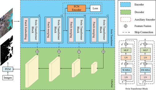
In this section, we present the WISTE as a novel semantic segmentation method for extracting water bodies from multispectral images. The overall architecture of the WISTE is shown in Figure 1. An encoder-decoder model structure is built, consisting of a dual-branch encoder and a single decoder. It should be noted that the encoder-decoder-based model can support more than three input channels. However, labeled data for more than three channels are difficult to obtain. The encoder part consists of the main Swin Transformer encoder and the auxiliary FCN encoder, which extract deep features from the input images. The input encoder data consist of three channels (e.g. RGB) of remote sensing images. To aggregate more global semantic information, the auxiliary encoder is embedded in the middle of the Swin Transformer. We merge the feature map between the encoder and decoder in a skip connection manner, which is inspired by ResNet (He et al. 2016). Skip connections are used in our method to avoid the gradient vanishing or gradient descent problems that may be caused by deep architectures. The original multispectral image and the segmentation results output by the decoder are input into the PME module simultaneously. First, the multispectral image is segmented based on the NDWI, and thus, a water body segmentation result is obtained. Then, the average posterior probability results are calculated after integrating individual classifiers based on the posterior probability of each classifier. Finally, the water maps predicted by the Swin Transformer and NDWI are combined, and final water extraction results are obtained.

Figure 1. Overall structure of the proposed WISTE method. The encoder part is shown in the blue box, and the decoder part is shown in the green box. The Swin Transformer block structure is shown in the lower-right part. The abbreviations MLP, LN, W-MSA, and SW-MSA denote a multilayer perceptron, layer normalization, window-based multihead self-attention, and shifted window-based multihead self-attention, respectively.

2.2. Swin Transformer

The Swin Transformer is a Transformer-based structure that utilizes a hierarchical design and a shifted window operation for calculating self-attention. The Swin Transformer model is trained through four stages, and the resolution of the feature map decreases gradually in each stage. Patch embedding is implemented at the beginning to cut the input images into patches. Patch merging works similarly to the pooling layer in a CNN, downsampling the input image to reduce its dimensionality. As shown in Figure 2a, elements are selected at intervals of two in the row and column directions of the input feature map and spliced into a tensor. After passing through the layer normalization operation and the fully connected layer, the H and W values of the feature map are cut in half, and C is doubled.

Figure 2. Main computation process of the Swin Transformer. (a) Patch merging to reduce the dimensionality of the feature map. The H, W, and C values of a patch denote the height, width, and number of channels of the corresponding feature map, respectively. (b) Hierarchical layer with different window sizes, with sampling levels of 4×, 8×, and 16×. (c) Window partitioning strategy in the Swin Transformer, where the semantic information between neighbouring patches is considered. (d) Shifted-window self-attention computation. The patches in dashed red boxes are masked, and self-attention is computed within the solid red boxes.

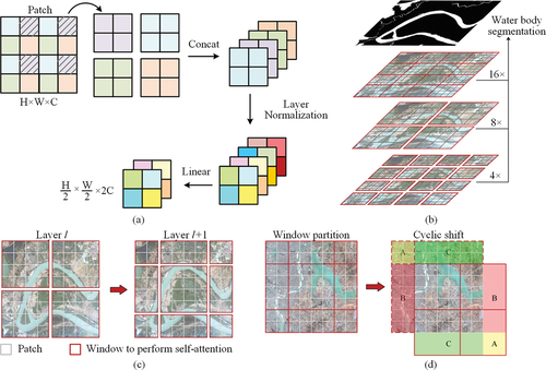
As shown in Figure 2b, the Swin Transformer builds a hierarchical representation by merging the neighboring patches in deep layers. These hierarchical feature maps are conveniently leveraged by the decoder part, such as the Unified Perceptual Network (UPerNet). Moreover, the self-attention computation only focuses on the local window (shown in gray), which has linear complexity instead of exponential complexity.

Performing window attention only in the red box for the Transformer leads to different window connection shortages, restricting the receptive field of the model. To better communicate semantic information between different windows, a shifted window is proposed for the Swin Transformer as shown in Figure 2c.

The Swin Transformer block is the core design of the overall structure, and two branches build up a complete block, as shown in Figure 1. In the I^th computation, the input feature map is divided into four parts by 4 × 4 windows. The self-attention operation is performed within each window. Layer l +1 contains nine windows after window partitioning, so the computational complexity of self-attention significantly increases. In addition, different window sizes lead to unfair feature extraction results. To solve the problems mentioned above, the cyclic shift operation is introduced, as shown in Figure 2d. Areas A and C are moved to the bottom, and then area B is moved to the right side. After performing cyclic shifting, the different areas are spliced together and form four new windows to perform self-attention. Although the cross-window semantic features are connected after the cyclic shift operation, this leads to a computational complexity increase. In addition, nonneighbouring areas (e.g. B and C) in the merged feature maps are merged in the same window to compute self-attention, which destroys the semantic relevance and obtains the wrong attention value. To handle the problem illustrated above and unify the self-attention computation, the Swin Transformer masks the moved and unmoved areas to prevent interference while computing the (l +1)^th self-attention value (Liu et al. 2021). After this calculation, moved areas A, B, and C are moved back to their original positions.

2.3. Dual-encoder architecture

As shown in Figure 3, we introduce an FCN as an auxiliary encoder with four convolutional blocks (e.g. Conv1 to Conv4). In the main branch, the weights W₁, … , W₄ are associated with four Swin Transformer layers. The auxiliary encoder is illustrated in the dashed box, and W_f3, … , W_f6 are the weights from Conv1 to Conv4, respectively. The parameters of the Swin Transformer branch and auxiliary branch can be represented by W and W_f, respectively:

Figure 3. Illustration of the dual-encoder architecture of the WISTE. The auxiliary encoder branch is indicated by a dashed red box. ST denotes the Swin Transformer; W_i represents the matrices for each computational block; x_i denotes the intermediate layer outputs; and L_i signifies the loss function of the corresponding branch.

(1) $W=\left(W_1,\dots ,\hspace{0.17em}{W}_4\right)$(1)

(2) $W_f=\left(W_{f3},\dots ,\hspace{0.17em}{W}_{f6}\right)$(2)

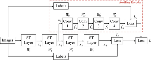
Feature map x₄ is input into the last softmax layer to compute the probability for each possible label m = 1, … , M, and the output of the softmax layer can be obtained by

(3) $p_m=\frac{exp\left(x_{4\left(k\right)}\right)}{\sum _{m=1}^{M}exp\left(x_{4\left(k\right)}\right)}$(3)

where x_4(k) is the k^th element of response x₄.

The corresponding loss function of the Swin Transformer branch can be given by:

(4) $L_0\left(W\right)=-\sum _{m=1}^M{y}_{m}log\left(p_m\right)$(4)

where p_m denotes the output of the softmax layer, y_m = 1 if the feature map has label m and y_m = 0 otherwise.

Similarly, given a feature map f₆ for the softmax layer of the auxiliary branch, the auxiliary loss can be given by:

(5) $L_s\left(W_f\right)=-\sum _{m=1}^M{y}_m\mathrm{l}\mathrm{o}\mathrm{g}\left(p_{wk}\right)$(5)

where p_wk denotes the output of the auxiliary softmax encoder. The combined loss L for the entire network can be given by a weighted sum of the main loss L₀(W) and the auxiliary loss L_s(W_s) as follows:

(6) $L\left(W,W_f\right)=L_0\left(W\right)+{\alpha }_t{L}_s\left(W,W_f\right)$(6)

The backpropagation effects of the main branch and auxiliary branch are balanced by a weighting factor α_t (Wang et al. 2015), where α decays as a function of the number of epochs t, with a total of N epochs. The initial value of α_t is set to 1.

(7) ${\alpha }_t={\alpha }_t\left(1-\frac{t}{N}\right)$(7)

2.4. Predicted map ensemble (PME) module

In the semantic segmentation task for remote sensing images, the current deep learning methods use three-channel inputs. When the input data are multispectral images, it is necessary to reduce the dimensionality of the data, which ignores the valid semantic information contained in the extra spectral bands. Therefore, we propose the PME module, which considers the water body probabilities of the NDWI. Motivated by ensemble learning (Sagi and Rokach 2018), the Swin Transformer and NDWI are considered two independent classifiers. The classification results of these two classifiers are embedded using the Bayesian combination strategy.

The NDWI is adopted as a water index to take advantage of the spectral features of the input data. Compared to other water indices, the NDWI is more suitable for remote sensing images with four bands (e.g. Gaofen-1/2, Worldview-2, and GeoEye-1). For multispectral remote sensing images, the NDWI can be calculated by (McFeeters 1996):

(8) $\mathrm{N}\mathrm{D}\mathrm{W}\mathrm{I}=\frac{\left(Green-NIR\right)}{\left(Green+NIR\right)}$(8)

The range of the NDWI is [−1, 1], and the values of the NDWI in water areas are generally larger than 0.5. Water bodies hardly reflect light in the near-infrared band, and the NDWI uses this characteristic to separate water areas from the background.

The Bayesian combination strategy (Kittler, Hater, and Duin 1998) is based on the observation that for a given pixel x_i in image X, the average posterior probability P_ave of each classifier can be calculated from the posterior probability estimate of each classifier. P_ave can be calculated as follows:

(9) $P_{ave}=\frac{1}{N}\sum _{k=1}^N{P}^k\left(C_i|x_i\right)$(9)

where P^k(C_i|x_i) is the estimate of the a posteriori probability of classifier k, N is the number of classifiers, and C is the number of categories (i.e. water and nonwater). The predictions yielded by the Swin Transformer can be represented as x = [x₁, x_2, … , x_m], and the water index values extracted from the NDWI can be represented as y = [y₁, y_2, … , y_m], where $m$ denotes the number of pixels.

The softmax function is used as the last layer of the Swin Transformer to compute the probability p(x_j) of each pixel j, which can be calculated by:

(10) $p_{\left(x_j\right)}=\frac{e^{x_j}}{\sum _{c=1}^C{e}^{x_c}}$(10)

The probability of each pixel according to the NDWI can be represented as p(y_j). Since the value range of the NDWI is [−1,1] and the value range of p(x_j) is [0,1], to calculate P_ave, min-max normalization is used to unify the value ranges of p(x_j) and p(y_j). The normalized p(y_j) can be denoted as:

(11) $p_{\left(y_j\right)}=\frac{NDW{I}_j-NDW{I}_{min}}{NDW{I}_{max}-NDW{I}_{min}}$(11)

where NDWI_min and NDWI_max denote the minimum and maximum NDWI values, respectively. NDWI_j denotes the NDWI value of jth pixel. It can be derived from Equation (9)(9) $P_{ave}=\frac{1}{N}\sum _{k=1}^N{P}^k\left(C_i|x_i\right)$(9) that P_ave here can be obtained with p(x_i) and p(y_i):

(12) $P_{ave}=\frac{1}{2}\left[p_{\left(x_j\right)}+p_{\left(y_j\right)}\right]$(12)

2.5. Loss function

The cross-entropy loss is a metric used to measure the difference between the ground-truth map and the predicted map. Compared to other loss functions such as the mean square error (MSE) and L1 losses, the cross-entropy loss function enables the network to have a faster gradient descent process during the initial phase of training and avoid gradient vanishing (Zhang and Sabuncu, 2018). In information theory, cross-entropy represents the divergence between two probability distributions j and k, where j denotes the true distribution and k denotes the predicted distribution. The cross-entropy loss L_CE can be given by:

(13) $L_{CE}\left(j,k\right)=-\sum _{i=1}^{n}j\left(x_i\right)\mathrm{l}\mathrm{o}\mathrm{g}\left(k\left(x_i\right)\right)$(13)

In terms of water body extraction tasks, j(x_i) is the ground-truth label, and k(x_i) is the predicted water body map. In binary classification tasks (e.g. water body extraction), the cross-entropy loss can be calculated by:

(14) $L_{CE}\left(j,k\right)=-\left[jlogk+\left(1-j\right)\mathrm{l}\mathrm{o}\mathrm{g}\left(1-k\right)\right]$(14)

The cross-entropy loss is generally employed with the softmax function to process the output feature map. The predicted values of multiple categories are summed to 1, and then the cross-entropy loss is calculated. The smaller the cross-entropy value is, the better the model predictions.

2.6. Evaluation metrics

Three widely used evaluation metrics are employed to evaluate the performance of our model, i.e. the F₁ score, overall accuracy (OA), and mean intersection over union (mIoU). The recall and precision metrics can be deduced from the confusion matrix, which contains true positive (TP), false positive (FP), true negative (TN), and false negative (FN). Then, the F₁ score can be obtained by:

(15) $\mathrm{P}\mathrm{r}\mathrm{e}\mathrm{c}\mathrm{i}\mathrm{s}\mathrm{i}\mathrm{o}\mathrm{n}=\frac{TP}{TP+FP}$(15)

(16) $\mathrm{R}\mathrm{e}\mathrm{c}\mathrm{a}\mathrm{l}\mathrm{l}=\frac{TP}{TP+FN}$(16)

(17) ${\mathrm{F}}_1=2\times \frac{\mathrm{P}\mathrm{r}\mathrm{e}\mathrm{c}\mathrm{i}\mathrm{s}\mathrm{i}\mathrm{o}\mathrm{n}\times \mathrm{R}\mathrm{e}\mathrm{c}\mathrm{a}\mathrm{l}\mathrm{l}}{\mathrm{P}\mathrm{r}\mathrm{e}\mathrm{c}\mathrm{i}\mathrm{s}\mathrm{i}\mathrm{o}\mathrm{n}+\mathrm{R}\mathrm{e}\mathrm{c}\mathrm{a}\mathrm{l}\mathrm{l}}$(17)

The overall accuracy refers to the ratio between what the model correctly predicts on all test sets and the overall dataset. The OA can be described as:

(18) $\mathrm{O}\mathrm{A}=\frac{TP}{TP+FP+FN+TN}$(18)

For each category, the IoU represents the ratio of the intersection and union between the predicted map and the ground-truth map, which can be calculated as:

(19) $\mathrm{I}\mathrm{o}\mathrm{U}=\frac{TP}{TP+FP+FN}$(19)

For the water body extraction task, TP denotes the number of pixels where both the ground truth and the predicted result are water bodies, while TP+FP+FN represents the number of pixels in their union area. Furthermore, the mIoU denotes the mean of the IoUs derived from all categories of remote sensing images.

3. Datasets

3.1. Data introduction

The Gaofen Image Dataset (GID) (Tong et al. 2020) is a large-scale semantic segmentation dataset composed of Gaofen-2 (GF-2) remote sensing images. Two panchromatic and multispectral sensors with spatial resolutions of 1 m and 4 m in the panchromatic and multispectral bands are onboard, respectively. The large-scale GID includes 150 high-spatial-resolution GF-2 images with image sizes of 7200 × 6800 collected from over 60 cities in China and contains five land use categories, including buildup, forest, farmland, meadows, and water.

The DeepGlobe Land Cover Classification Challenge dataset comes from a land cover classification competition hosted by DeepGlobe (Demir et al. 2018). Over 800 remote sensing images are provided with image sizes of 2448 × 2448. The imagery has a 0.5-m pixel resolution and was collected by DigitalGlobe’s satellites. Seven categories, including urban, agricultural, grassland, forest, water, barren, and background areas, are labeled.

3.2. Data preprocessing

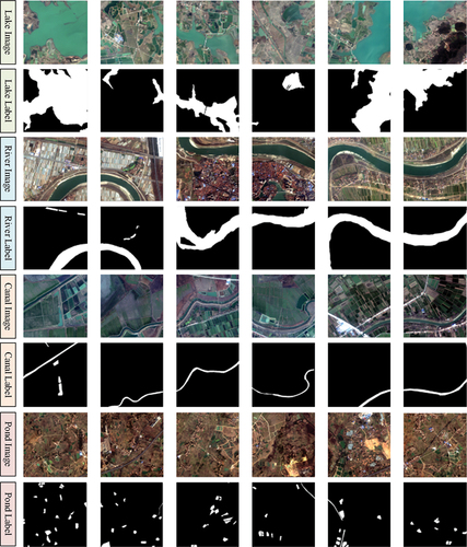
The water datasets mentioned in Section 3.1 are cropped to 512$\times$512 pixels for both images and labels. After cropping, the GID dataset contains 35,991 samples, and the DeepGlobe dataset contains 10,559 samples. Each category is labeled at the pixel level, and areas not belonging to these categories are labeled as background areas, as shown in Figure 4. To enhance the generalization of the model, horizontal, vertical, and horizontal and vertical flips are used for geometric data augmentation, and photometric distortion is used for color data augmentation. Photometric distortion adjusts the brightness, chroma, contrast, and saturation of images while adding noise to. After completing data augmentation, we obtain a water dataset with a total of 175,632 samples. We divide all samples into training samples and validation samples at a ratio of 4:1, with 140,505 samples for model training and 35,127 samples for model validation. As illustrated in Figure 5, the overall dataset contains four different water types, including lakes, rivers, canals, and ponds.

Figure 4. Images land cover labels and corresponding water body extraction labels of two public datasets, i.e. (a) The GID and (b) DeepGlobe dataset.

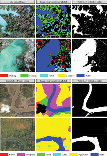
Figure 5. Images and labels of different water types contained in the GID dataset. From top to bottom, the rows present lakes, rivers, canals, and ponds.

4. Experiments and results

4.1. Environmental settings

This experiment is performed in a server environment (with an Intel Core i7 12700K CPU and two NVIDIA RTX 2080Ti GPUs). All experiments are implemented based on Python 3.8 and the PyTorch 1.11.0 deep learning framework, and CUDA 11.5 is used to accelerate the training and inference processes. MMCV 1.6.0 and MMSegmentation 0.26.0 are employed to execute the Transformer-based model.

4.2. Ablation studies

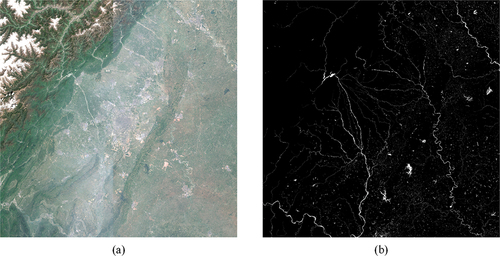
To evaluate the performance of the WISTE in large-scale water extraction tasks, we compare the single-encoder model and the dual-encoder model of the Swin Transformer. In addition, we explore the effectiveness of our proposed PME module through a controlled experiment. The Swin Transformer with a single-branch encoder is employed as the baseline network. Since the images in the DeepGlobe dataset are three-band images, which do not satisfy the PME module, a publicly available labeled Sentinel-2 image is adopted (Yuan et al. 2021), as depicted in Figure 6. Sentinel-2 is the second satellite of ESA’s Copernicus Programme. It contains 13 bands with a 290-km width and a 10-m spatial resolution for the blue (B2), green (B3), red (B4), and near-infrared (B8) channels.

Figure 6. One Sentinel-2 image used for ablation experiments. (a) Sentinel-2 image obtained after band fusion (B2, B3, B4 and B8 for the B, G, R, and NIR bands, respectively). (b) Ground truth of the water body, with water in white and the background in black.

The results of the ablation experiments are presented in Table 1. To demonstrate the efficacy of the dual-encoder architecture, popular feature extractors, i.e. UPerNet and an FCN, are used as auxiliary encoders. Clearly, each auxiliary encoder model can effectively improve the water body extraction performance achieved by the network. Specifically, ST-UPer and ST-FCN increase the mIoU by 1.48% and 2.36%, respectively, over that of the original Swin Transformer using the GID. It can be seen that the dual-encoder architecture is more powerful for semantic information extraction. Moreover, as an auxiliary encoder, the FCN exhibits a better feature extraction ability than UPerNet using both datasets. Compared with those of the original ST, the mIoUs of ST-PME increase by 1.65% and 0.95% using the GID and Sentinel-2 images, respectively. The results of the WISTE experiment shown in the last row demonstrate that the dual-encoder and PME module yield significantly improved segmentation performance over that of the ST baseline. The WISTE enhances the mIoUs by 4.3% and 2.49% on GID and Sentinel-2, respectively, over those of the original ST. In addition, the WISTE obtains the best evaluation metrics in comparisons with ST-FCN and ST-PME, demonstrating that the WISTE is more effective for water body extraction than the single-enhancement strategy.

Table 1. Ablation experiment results obtained by the proposed WISTE on the GID and Sentinel-2 images (the best values are in bold).

Method	Dual-Encoder	PME	GID			Sentinel-2
			F1 (%)	mIoU (%)	OA (%)	F1 (%)	mIoU (%)	OA (%)
Original ST^1			94.52	86.77	96.25	75.63	64.87	82.24
ST-UPer	√		95.29	88.25	97.07	77.52	65.23	84.16
ST-FCN	√		97.64	89.13	97.85	78.06	65.57	85.53
ST-PME		√	97.80	88.42	96.39	78.51	65.82	85.95
WISTE	√	√	98.91	91.07	98.88	79.54	67.36	86.78

¹Swin Transformer with a single encoder branch.

4.3. Comparison with other methods

To further evaluate the performance of the dual-encoder architecture in the Swin Transformer, we compare the proposed ST-Dual model with several CNN-based models, including DeepLab v3+ (Duan et al. 2021), D-LinkNet (Zhou et al. 2018), the dual-attention network (DANet) (Chen et al. 2021), and the original Swin Transformer (Panboonyuen et al. 2021). The CNN-based methods mentioned above all use ResNet-34 as the backbone network, while the Swin Transformer and ST-Dual adopt the ADE-20K pretrained model “Swin-B” as the backbone. Due to GPU memory limitations, the original DeepGlobe images are split into 512 × 512 patches for inference.

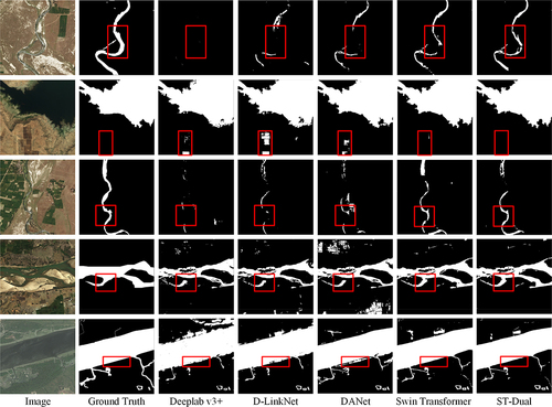
The experimental results produced by different models on the DeepGlobe dataset are illustrated in Figure 7. We select five images that include typical water types (small canals, diked rivers, braided rivers, etc.). The model extraction results obtained based on CNN are insufficient. As shown in the 1^st and 3^rd rows, when the spatial features are not obvious, DeepLab v3+ can hardly extract effective features, making it difficult to extract water boundaries. D-LinkNet has a larger receptive field than DeepLab v3+ due to its atrous convolution structure (Chen et al. 2018), and its extraction results are more comprehensive, but obvious misclassifications still occur. The DANet introduces a dual-branch attention module based on atrous convolution, which further improves its feature extraction ability. The water body segmentation results of the Swin Transformer are significantly superior to those of the CNN-based models, with no apparent misclassifications and smooth river boundaries, demonstrating the Transformer’s powerful semantic information extraction capabilities. In addition, the Swin Transformer can extract water bodies in areas with weak spatial information (see the 3^rd row in Figure 7). The ST-Dual model has the best prediction results and achieves good results for each water category. ST-Dual introduces an FCN as an auxiliary encoder, which enhances its global modeling capability compared to that of the Swin Transformer with a single encoder. As shown in the 1^st and 3^rd rows, ST-Dual can extract small rivers more completely and minimize the missing spatial details extracted from remote sensing images.

Figure 7. Comparison among the prediction results produced by different methods on the DeepGlobe dataset. The water areas are in white, while the background is in black. The red boxes highlight areas with weak spatial information.

We evaluate the number of parameters, inference time, and accuracy metrics of each model, as listed in Table 2. The number of parameters refers to the size of the trained model file. ST-Dual achieves the highest accuracy on the DeepGlobe dataset. Compared with the Swin Transformer, ST-Dual improves the F1, mIoU, and OA values by 1.41%, 1.89%, and 1.66%, respectively. In addition, the inference times and numbers of parameters required by ST-Dual and the Swin Transformer are equivalent, which indicates that the dual-encoder structure does not demand an extra inference overhead. Although the inference time of DeepLab v3+ is the shortest, atrous spatial pyramid pooling (ASPP) has difficulty capturing useful information in weak semantic areas (e.g. the 1^st and 3^rd rows in Figure 7). ST-Dual improves the F1 score by 4.25%, the mIoU by 4.39%, and the OA by 7.1% over those of DeepLab v3+, which demonstrates that the dual-encoder architecture is more effective for global context modeling and can achieve better semantic segmentation results.

Table 2. Comparison among the different methods on the DeepGlobe dataset (the best values are in bold).

Method	Parameters (MB)^2	Time (s)	F1(%)	mIoU (%)	OA (%)
DeepLab v3+	42.21	37.06	86.39	73.52	85.47
D-LinkNet	46.7	35.47	86.87	73.43	86.63
DANet	45.92	42.58	87.65	74.27	88.71
Swin Transformer	88.2	73.54	89.23	76.02	90.91
ST-Dual^1	89.5	75.16	90.64	77.91	92.57

¹Swin Transformer with a dual-encoder architecture. ² Parameter file size in megabytes.

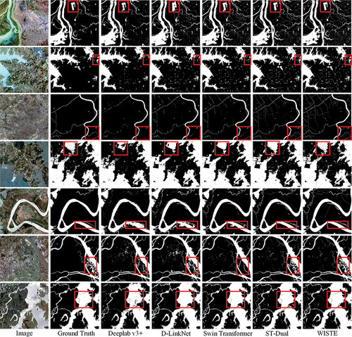
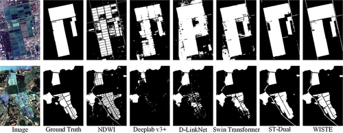
Furthermore, to evaluate performance of the proposed WISTE, we compare it with DeepLab v3+, D-LinkNet, the Swin Transformer, and ST-Dual on the multispectral GID. Seven typical images containing different types of water areas are illustrated in Figure 8. The areas where the WISTE demonstrates greater advantages are highlighted in red boxes. It can be observed that DeepLab v3+ is insufficient for global modeling, leading to many semantic fragments in its water extraction results. In mixed water-background areas (e.g. the 2^nd and 6^th rows), D-LinkNet has difficulty extracting useful information for water segmentation, which leads to incomplete water extraction results. The original Swin Transformer is capable of extracting complete water areas (see, e.g. the 4^th and 7^th rows) due to its shifted window attention module but has difficulties extracting small streams with limited semantic information (e.g. the 3^rd row). Compared with the Swin Transformer, ST-Dual is more adept at extracting spatial features and capturing more useful features for segmentation. The prediction results of the WISTE are much closer to the ground truth, and the segmentation errors are effectively reduced. Moreover, the PME module improves the discriminative ability of the network for some water areas with nonwater spatial features (e.g. the 6^th row).

Figure 8. Comparison among the prediction results produced by different methods using the GID. The water areas are drawn in white. The areas where the WISTE demonstrates greater advantages are highlighted in red boxes.

The statistical results of each segmentation method are displayed in Table 3. The proposed WISTE method achieves the best results in terms of all three metrics, i.e. F1, the mIoU, and the OA, with values of 98.69%, 90.36%, and 98.75%, respectively. Moreover, the WISTE improves the F1 score by 4.17%, the mIoU by 3.59%, and the OA by 2.5% over those of the original Swin Transformer, but the inference time only increases by 6.23 s. Due to the image quality and spatial water feature advantages of the GID over DeepGlobe, the mIoU achieved by each method on the GID is generally higher than that obtained on the DeepGlobe dataset (Table 2 vs. Table 3). It can be revealed that the segmentation results of the Transformer-based models significantly surpass those of the CNN-based models, as shown in Table 3, which proves that CNN-based models have shortcomings in terms of representing global semantic features.

Table 3. Comparison among the different methods on the GID dataset (the best values are in bold).

Method	Parameters (MB)	Time (s)	F1 (%)	mIoU (%)	OA (%)
DeepLab v3+	42.21	43.04	86.69	72.56	89.64
D-LinkNet	46.7	45.21	88.04	73.91	90.61
Original ST	45.92	62.54	94.52	86.77	96.25
ST-Dual	88.2	64.27	97.64	89.13	97.85
WISTE	89.5	68.77	98.69	90.36	98.75

We select two typical regions with complex spatial water features for water body extraction to further verify the competence of our proposed WISTE. The segmentation results of different models are shown in Figure 9. Despite adopting an ASPP or atrous convolution strategy, the CNN-based DeepLab v3+ and D-LinkNet models are insufficient for the extraction of water information. The dual-encoder ST-Dual model exhibits greater potential for global context modeling, and its segmentation result is more complete. The WISTE extracts spectral features from the NDWI and combines them with spatial features, which further improves its water body segmentation results, as illustrated in Figure 9. According to the WISTE visualization results, the PME module effectively perceives pixel-level features, in which intraboundaries and extraboundaries are extracted with great advantages.

Figure 9. In-detail comparison among the prediction results produced by different methods on the GID dataset.

5. Discussion

In this study, to effectively map water bodies in multispectral remote sensing images, an automatic deep learning-based method is proposed. A Swin Transformer with a dual-branch encoder architecture is designed, and a FCN is adopted as an auxiliary encoder to capture more semantic information. To alleviate the model’s dependence on spatial features and make full use of spectral information, we propose a predicted map ensemble module. The average posterior probability of each classifier is calculated after the ensembling step to determine the final category of each pixel. Experimental results obtained on the GID and the DeepGlobe dataset show that the WISTE achieves higher performance (e.g. F1, mIoU, and OA values) than other methods.

We compare different arrangements of the GID dataset for effectively utilizing multispectral data. Five different training sample combinations (i.e. RGB, NGB, RNG, RGN, and RGBN) are designed, as shown in Table 4. Original ST refers to the Swin Transformer with a single encoder branch. Time refers to the average time required to infer an image. It can be seen that the RGBN strategy obtains the best mIoU in both the original ST and WISTE methods. However, the inference time of RGBN is over 20 seconds longer than those of the other combinations. The RGB strategy achieves the highest mIoU with the combination of the three bands. In addition, the RGB result is closest to the mIoU of RGBN (i.e. the differences are 0.30 and 0.31 for original ST and the WISTE, respectively). Considering the time consumption and accuracy index, RGB is adopted as the training sample strategy.

Table 4. Different band arrangements of the training samples in the GID dataset (the best values are in bold).

Method	RGB		NGB		RNB		RGN		RGBN
	Time (s)	mIoU (%)	Time (s)	mIoU (%)	Time (s)	mIoU (%)	Time (s)	mIoU (%)	Time (s)	mIoU (%)
Original ST^1	62.54	86.47	62.01	85.60	63.58	85.34	60.74	86.06	83.67	86.77
WISTE	64.69	89.81	64.69	88.46	65.57	86.98	63.97	88.87	88.24	90.12

¹Swin Transformer with a single encoder branch.

The WISTE ensembles the auxiliary encoder in the Swin Transformer to reduce the number of additional parameters. As shown in Figure 3, the first two Transformer layers acquire the relationships between neighboring pixels, and then the FCN is embedded for global contextual modeling. Table 5 depicts the segmentation results obtained with different auxiliary encoder positions. The experimental results show that different positions (e.g. $\hspace{0.17em}{x}_1$, $\hspace{0.17em}{x}_2$, $\hspace{0.17em}{x}_3$, and $\hspace{0.17em}{x}_4$) of the FCN affect the performance of the dual-encoder structure, where $x_2$ is the optimal position for ensembling the FCN encoder with the Swin Transformer. Moreover, the method integrating the FCN outperforms the original ST at all locations. In addition, the WISTE can also be applied to multiresolution satellite images. Expanded experiments supporting this notion are given in the supplementary material.

Table 5. Relationships between different FCN positions and the accuracy of ST-Dual (the best values are in bold).

Method	GID			DeepGlobe
	F1 (%)	mIoU (%)	OA (%)	F1%)	mIoU (%)	OA (%)
Original ST	94.52	86.77	96.25	89.23	76.02	90.91
ST-Dual^x1	95.46	88.76	96.52	89.49	76.73	90.88
ST-Dual^x2	97.64	89.13	97.85	90.64	77.91	92.57
ST-Dual^x3	96.07	88.34	96.67	89.68	77.21	91.63
ST-Dual^x4	95.37	88.16	96.33	89.54	76.85	91.24

The misclassification of dark surfaces (e.g. mountain shadows and asphalt pavement) as water bodies is a challenge in the water body extraction task (Liu et al. 2023; Wang et al. 2023), and the similar spatial features of dark water bodies and dark surfaces pose difficulties for deep learning models. When the input data are multispectral images, due to the different surface reflectances between different features, it is possible to exclude features with similar characteristics based on the water body index. However, when the data source is only a three-channel image, other features (e.g. boundaries and contours) are needed to distinguish these water bodies or to design neural networks with more characterization capabilities for learning these subtle differences (Tayer et al. 2023).

Although our proposed WISTE method achieves good segmentation performance on the GID and the DeepGlobe dataset, it still exhibits some deficiencies that will guide our future research. On the one hand, Swin Transformer-based models usually have large numbers of parameters, which results in very expensive training and deployment costs. It is necessary to adopt model distillation to achieve improved efficiency. On the other hand, as an auxiliary encoder, the FCN is not sufficiently sensitive to detailed features, which leads to less smooth water boundary lines. We will consider other pixel-level encoders in future work.

6. Conclusion

In this article, a Water Index and Swin Transformer ensemble (WISTE) method is proposed for performing water body mapping on multispectral remote sensing images. The novelty of the WISTE lies in its dual-branch encoder architecture designed based on the Swin Transformer, as well as its predicted map ensemble module. The former adopts an FCN as an auxiliary encoder for global contextual modeling. The latter combines results derived from the Swim Transformer and a water index (i.e. NDWI) to reduce uncertainty. Evaluating the WISTE on the GID and the DeepGlobe dataset, the results demonstrate that the WISTE achieves excellent water body extraction performance in comparison with other methods, such as DeepLab v3+, D-LinkNet, DANet, and the original Swin Transformer. Compared with the original Swin Transformer, our proposed method improves the F1, mIoU, and OA values by 1.41%, 1.89%, and 1.66% on the DeepGlobe dataset and by 4.17%, 3.59%, and 2.5% on the GID, respectively. Moreover, the WISTE has comparable inference time overhead to that of the Swin Transformer, which demonstrates that our method is more efficient while maintaining high accuracy.

Authorship contribution statement

Donghui Ma: Conceptualization, Methodology, Software, Writing-original draft preparation, Writing-review and editing. Liguang Jiang: Conceptualization, Methodology, Writing-review and editing, Supervision, Project administration. Jie Li: Analysis of the datasets and experimental results. Yun Shi: Writing-review and editing.

Code availability section

Name of the method: Water Index and Swin Transformer Ensemble (WISTE)

Contact: [email protected]

Hardware requirements: NVIDIA RTX A6000 × 2

Programming language: Python 3.8.13

Software needed: PyTorch 1.11.0, mmsegmentation 0.26.0, opencv-python 4.6.0.66

Program size: 31 M

The source codes are available for download at the following link: https://github.com/xxx7913586/WISTE

Acknowledgments

This work was partially supported by the Shenzhen Key Laboratory of Precision Measurement and Early Warning Technology for Urban Environmental Health Risks (ZDSYS20220606100604008), SUSTech research start-up grants (Y01296129; Y01296229), the CRSRI Open Research Program (Program SN: CKWV20221009/KY) and the Natural Science Foundation of China (no. 42174045; no. 41874012).

Disclosure statement

No potential conflict of interest was reported by the author(s).

Data availability statement

The datasets used in this study are publicly available. The Gaofen Image Dataset (GID) is available at https://x-ytong.github.io/project/GID.html, and the DeepGlobe dataset is downloadable at https://competitions.codalab.org/competitions/18468

Supplementary Material

Supplemental data for this article can be accessed online at https://doi.org/10.1080/15481603.2023.2251704

Additional information

Funding

The Shenzhen Key Laboratory of Precision Measurement and Early Warning Technology for Urban Environmental Health Risks [ZDSYS20220606100604008]; the CRSRI Open Research Program [Program SN: CKWV20221009/KY]; Natural Science Foundation of China [No. 42174045; No. 41874012]; and the SUSTech research start-up grants [Y01296129; Y01296229].

References

- An, S. H., and X. P. Rui. 2022. “A High-Precision Water Body Extraction Method Based on Improved Lightweight U-Net.” Remote Sensing 14 (17): 4127. https://doi.org/10.3390/rs14174127.
- Bahdanau, D., K. Cho, and Y. Bengio. 2014. “Neural Machine Translation by Jointly Learning to Align and Translate.” arXiv Preprint arXiv 1409:0473. https://doi.org/10.48550/arXiv.1409.0473.
- Belgiu, M., and L. Dragut. 2016. “Random Forest in Remote Sensing: A Review of Applications and Future Directions.” Isprs Journal of Photogrammetry & Remote Sensing 114:24–17. https://doi.org/10.1016/j.isprsjprs.2016.01.011.
- Chen, L. C., G. Papandreou, I. Kokkinos, K. Murphy, and A. L. Yuille. 2018. “DeepLab: Semantic Image Segmentation with Deep Convolutional Nets, Atrous Convolution, and Fully Connected CRFs.” IEEE Transactions on Pattern Analysis & Machine Intelligence 40 (4): 834–848. https://doi.org/10.1109/tpami.2017.2699184.
- Chen, X., C. P. Qiu, W. Y. Guo, A. Z. Yu, X. C. Tong, and M. Schmitt. 2022. “Multiscale Feature Learning by Transformer for Building Extraction from Satellite Images.” IEEE Geoscience & Remote Sensing Letters 19:1–5. https://doi.org/10.1109/lgrs.2022.3142279.
- Chen, J., Z. Y. Yuan, J. Peng, L. Chen, H. Z. Huang, J. W. Zhu, Y. Liu, and H. F. Li. 2021. “DASNet: Dual Attentive Fully Convolutional Siamese Networks for Change Detection in High-Resolution Satellite Images.” IEEE Journal of Selected Topics in Applied Earth Observations & Remote Sensing 14:1194–1206. https://doi.org/10.1109/jstars.2020.3037893.
- Demir, I., K. Koperski, D. Lindenbaum, G. Pang, J. Huang, S. Bast, F. Hughes, D. Tuia, R. Raskar, and Ieee. 2018. “DeepGlobe 2018: A Challenge to Parse the Earth Through Satellite Images.” IEEE/CVF Conference on Computer Vision and Pattern Recognition (CVPR). IEEE Computer Society Conference on Computer Vision and Pattern Recognition Workshops, Salt Lake City, UT, 172–181. https://doi.org/10.1109/cvprw.2018.00031.
- Duan, Y. M., W. Y. Zhang, P. Huang, G. J. He, and H. X. Guo. 2021. “A New Lightweight Convolutional Neural Network for Multi-Scale Land Surface Water Extraction from GaoFen-1D Satellite Images.” Remote Sensing 13 (22): 4576. https://doi.org/10.3390/rs13224576.
- Feyisa, G. L., H. Meilby, R. Fensholt, and S. R. Proud. 2014. “Automated Water Extraction Index: A New Technique for Surface Water Mapping Using Landsat Imagery.” Remote Sensing of Environment 140:23–35. https://doi.org/10.1016/j.rse.2013.08.029.
- He, K., X. Zhang, S. Ren, and J. Sun. 2016. “Deep Residual Learning for Image Recognition.” Proceedings of the IEEE conference on computer vision and pattern recognition, 770–778. Las Vegas, NV, USA. https://doi.org/10.1109/CVPR.2016.90.
- Huang, X., T. Hu, J. Y. Li, Q. Wang, and J. A. Benediktsson. 2018. “Mapping Urban Areas in China Using Multisource Data with a Novel Ensemble SVM Method.” IEEE Transactions on Geoscience and Remote Sensing: A Publication of the IEEE Geoscience and Remote Sensing Society 56 (8): 4258–4273. https://doi.org/10.1109/tgrs.2018.2805829.
- Kittler, M. H., R. P. W. Duin, and J. Matas. 1998. “On combining classifiers.” IEEE Transactions on Pattern Analysis & Machine Intelligence 20 (3): 226–239. https://doi.org/10.1109/34.667881.
- Koda, S., A. Zeggada, F. Melgani, and R. Nishii. 2018. “Spatial and Structured SVM for Multilabel Image Classification.” IEEE Transactions on Geoscience and Remote Sensing: A Publication of the IEEE Geoscience and Remote Sensing Society 56 (10): 5948–5960. https://doi.org/10.1109/tgrs.2018.2828862.
- Li, X., D. Long, B. R. Scanlon, M. E. Mann, X. Li, F. Tian, Z. Sun, and G. Wang. 2022. “Climate Change Threatens Terrestrial Water Storage Over the Tibetan Plateau.” Nature Climate Change 12 (9): 1–7. https://doi.org/10.1038/s41558-022-01443-0.
- Liu, B., S. Du, L. Bai, S. Ouyang, H. Wang, and X. Zhang. 2023. “Water Extraction from Optical High-Resolution Remote Sensing Imagery: A Multi-Scale Feature Extraction Network with Contrastive Learning.” GIScience & Remote Sensing 60 (1): 2166396. https://doi.org/10.1080/15481603.2023.2166396.
- Liu, Z., Y. T. Lin, Y. Cao, H. Hu, Y. X. Wei, Z. Zhang, S. Lin, and B. N. Guo, Ieee. 2021. “Swin Transformer.” Hierarchical Vision Transformer using Shifted Windows, 18th IEEE/CVF International Conference on Computer Vision (ICCV), Electr Network, 9992–10002. https://doi.org/10.1109/iccv48922.2021.00986.
- Li, L. W., Z. Yan, Q. Shen, G. Cheng, L. R. Gao, and B. Zhang. 2019. “Water Body Extraction from Very High Spatial Resolution Remote Sensing Data Based on Fully Convolutional Networks.” Remote Sensing 11 (10): 1162. https://doi.org/10.3390/rs11101162.
- Lu, M., L. Y. Fang, M. X. Li, B. Zhang, Y. Zhang, and P. Ghamisi. 2022. “NFANet: A Novel Method for Weakly Supervised Water Extraction from High-Resolution Remote-Sensing Imagery.” IEEE Transactions on Geoscience & Remote Sensing 60:1–14. https://doi.org/10.1109/tgrs.2022.3140323.
- McFeeters, S. K. 1996. “The Use of the Normalized Difference Water Index (NDWI) in the Delineation of Open Water Features.” International Journal of Remote Sensing 17 (7): 1425–1432. https://doi.org/10.1080/01431169608948714.
- Mekhalfi, M. L., C. Nicolo, Y. Bazi, M. M. Al Rahhal, N. A. Alsharif, and E. Al Maghayreh. 2022. “Contrasting YOLOv5, Transformer, and EfficientDet Detectors for Crop Circle Detection in Desert.” IEEE Geoscience & Remote Sensing Letters 19:1–5. https://doi.org/10.1109/lgrs.2021.3085139.
- Miao, Z., K. Fu, H. Sun, X. Sun, and M. Yan. 2018. “Automatic Water-Body Segmentation from High-Resolution Satellite Images via Deep Networks.” IEEE Geoscience and Remote Sensing Letters 15 (4): 602–606. https://doi.org/10.1109/LGRS.2018.2794545.
- Ovakoglou, G., I. Cherif, T. K. Alexandridis, X.-E. Pantazi, A.-A. Tamouridou, D. Moshou, X. Tseni, I. Raptis, S. Kalaitzopoulou, and S. Mourelatos. 2021 . “Automatic detection of surface-water bodies from Sentinel-1 images for effective mosquito larvae control.” Journal of Applied Remote Sensing 15 (1): 014507. https://doi.org/10.1117/1.JRS.15.014507.
- Panboonyuen, T., K. Jitkajornwanich, S. Lawawirojwong, P. Srestasathiern, and P. Vateekul. 2021. “Transformer-Based Decoder Designs for Semantic Segmentation on Remotely Sensed Images.” Remote Sensing 13 (24): 5100. https://doi.org/10.3390/rs13245100.
- Pickens, A. H., M. C. Hansen, S. V. Stehman, A. Tyukavina, P. Potapov, V. Zalles, and J. Higgins. 2022. “Global Seasonal Dynamics of Inland Open Water and Ice.” Remote Sensing of Environment 272:272. https://doi.org/10.1016/j.rse.2022.112963.
- Rokni, K., A. Ahmad, A. Selamat, and S. Hazini. 2014. “Water Feature Extraction and Change Detection Using Multitemporal Landsat Imagery.” Remote Sensing 6 (5): 4173–4189. https://doi.org/10.3390/rs6054173.
- Sabatini, F. M., B. Jimenez-Alfaro, U. Jandt, M. Chytry, R. Field, M. Kessler, J. Lenoir, et al. 2022. “Global Patterns of Vascular Plant Alpha Diversity.” Nature Communications 13 (1). https://doi.org/10.1038/s41467-022-32063-z.
- Sagi, O., and L. Rokach. 2018. “Ensemble Learning: A Survey.” Wiley Interdisciplinary Reviews: Data Mining and Knowledge Discovery 8 (4): e1249. https://doi.org/10.1002/widm.1249.
- Sawaya, K. E., L. G. Olmanson, N. J. Heinert, P. L. Brezonik, and M. E. Bauer. 2003. “Extending Satellite Remote Sensing to Local Scales: Land and Water Resource Monitoring Using High-Resolution Imagery.” Remote Sensing of Environment 88 (1–2): 144–156. https://doi.org/10.1016/j.rse.2003.04.006.
- Song, J. H., Y. Wang, Z. C. Fang, L. Peng, and H. Y. Hong. 2020. “Potential of Ensemble Learning to Improve Tree-Based Classifiers for Landslide Susceptibility Mapping.” IEEE Journal of Selected Topics in Applied Earth Observations & Remote Sensing 13:4642–4662. https://doi.org/10.1109/jstars.2020.3014143.
- Sun, L., G. R. Zhao, Y. H. Zheng, and Z. B. Wu. 2022. “Spectral–Spatial Feature Tokenization Transformer for Hyperspectral Image Classification.” IEEE Transactions on Geoscience & Remote Sensing 60:1–14. https://doi.org/10.1109/tgrs.2022.3144158.
- Tayer, T. C., M. M. Douglas, M. C. R. Cordeiro, A. D. N. Tayer, J. N. Callow, L. Beesley, D. McFarlane, et al. 2023. “Improving the Accuracy of the Water Detect Algorithm Using Sentinel-2, Planetscope and Sharpened Imagery: A Case Study in an Intermittent River.” GIScience & Remote Sensing 60 (1): 2168676. https://doi.org/10.1080/15481603.2023.2168676.
- Tong, X. Y., G. S. Xia, Q. K. Lu, H. F. Shen, S. Y. Li, S. C. You, and L. P. Zhang. 2020. “Land-Cover Classification with High-Resolution Remote Sensing Images Using Transferable Deep Models.” Remote Sensing of Environment 237:237. https://doi.org/10.1016/j.rse.2019.111322.
- Vaswani, A., N. Shazeer, N. Parmar, J. Uszkoreit, L. Jones, A. N. Gomez, Ł. Kaiser, and I. Polosukhin. 2017. Attention is all you need. In Proceedings of the 31st International Conference on Neural Information Processing Systems (NIPS'17), 6000–6010. Red Hook, NY, USA: Curran Associates Inc.
- Wang, Y., G. Foody, X. Li, Y. Zhang, P. Zhou, and Y. Du. 2023. “Regression-Based Surface Water Fraction Mapping Using a Synthetic Spectral Library for Monitoring Small Water Bodies.” GIScience & Remote Sensing 60 (1): 2217573. https://doi.org/10.1080/15481603.2023.2217573.
- Wang, L., C. Y. Lee, Z. Tu, and S. Lazebnik. 2015. “Training Deeper Convolutional Networks with Deep Supervision.”
- Weng, Q. 2012. “Remote Sensing of Impervious Surfaces in the Urban Areas: Requirements, Methods, and Trends.” Remote Sensing of Environment 117:34–49. https://doi.org/10.1016/j.rse.2011.02.030.
- Xu, N., Y. Ma, H. Zhou, W. H. Zhang, Z. Y. Zhang, and X. H. Wang. 2022. “A Method to Derive Bathymetry for Dynamic Water Bodies Using ICESat-2 and GSWD Data Sets.” IEEE Geoscience & Remote Sensing Letters 19:1–5. https://doi.org/10.1109/lgrs.2020.3019396.
- Xu, Z. Y., W. C. Zhang, T. X. Zhang, Z. F. Yang, and J. Y. Li. 2021. “Efficient Transformer for Remote Sensing Image Segmentation.” Remote Sensing 13 (18): 3585. https://doi.org/10.3390/rs13183585.
- Yuan, K. H., X. Zhuang, G. Schaefer, J. X. Feng, L. Guan, and H. Fang. 2021. “Deep-Learning-Based Multispectral Satellite Image Segmentation for Water Body Detection.” IEEE Journal of Selected Topics in Applied Earth Observations & Remote Sensing 14:7422–7434. https://doi.org/10.1109/jstars.2021.3098678.
- Yu, L., Z. Y. Wang, S. W. Tian, F. Y. Ye, J. L. Ding, and J. Kong. 2017. “Convolutional Neural Networks for Water Body Extraction from Landsat Imagery.” International Journal of Computational Intelligence and Applications 16 (1): 1750001. https://doi.org/10.1142/s1469026817500018.
- Zhang, Z. L., M. Lu, S. P. Ji, H. F. Yu, and C. H. Nie. 2021. “Rich CNN Features for Water-Body Segmentation from Very High Resolution Aerial and Satellite Imagery.” Remote Sensing 13 (10): 1912. https://doi.org/10.3390/rs13101912.
- Zhou, L. C., C. Zhang, M. Wu, and Ieee. 2018. “D-Linknet: LinkNet with Pretrained Encoder and Dilated Convolution for High Resolution Satellite Imagery Road Extraction.” IEEE/CVF Conference on Computer Vision and Pattern Recognition (CVPR). IEEE Computer Society Conference on Computer Vision and Pattern Recognition Workshops, Salt Lake City, UT, 192–196. https://doi.org/10.1109/cvprw.2018.00034.