Performance, effectiveness and computational efficiency of powerline extraction methods for quantifying ecosystem structure from light detection and ranging

ABSTRACT

National and regional data products of the ecosystem structure derived from airborne laser scanning (ALS) surveys with Light Detection And Ranging (LiDAR) technology are essential for ecology, biodiversity, and ecosystem monitoring. However, noises like powerlines often remain, hindering the accurate measurement of 3D ecosystem structures from LiDAR. Currently, there is a lack of studies assessing powerline noise removal in the context of generating data products of ecosystem structures from ALS point clouds. Here, we assessed the (1) performance and accuracy, (2) effectiveness, and (3) time efficiency and execution time of three powerline extraction methods (i.e. two point-based methods based on deep learning and eigenvalue decomposition, respectively, and one hybrid method) for removing powerline noise when quantifying 3D ecosystem structures in landscapes with varying canopy heights and vegetation openness. Twenty-five LiDAR metrics representing three key dimensions of the ecosystem structure (i.e. vegetation height, cover, and vertical variability) across 10 study areas in the Netherlands were used for our assessment. The deep learning method had the best performance and showed the highest accuracy of powerline removal across various landscape types (average $F1$ score = 96%), closely followed by the hybrid method (average $F1$ score = 95%). In contrast, the accuracy of the eigenvalue decomposition method was lower (average $F1$ score = 82%) and depended on landscape context and vegetation composition (e.g. the $F1$ score decreased from 96% to 63% when the average canopy height increased across landscapes). Powerline noise removal had the highest effectiveness (i.e. generating LiDAR metrics closest to those derived from manually labeled ground truth data) for LiDAR metrics capturing height and cover of low- and high-vegetation layers. Time efficiency (processed points per second) was highest for the eigenvalue decomposition method, yet the hybrid method reduced the execution time by > 50% compared to the deep learning method (ranging from 20% to 89% in study areas with different landscape composition). Based on our findings, we recommend the hybrid method for upscaling powerline removal on multi-terabyte ALS datasets to a regional or national extent because of its high accuracy and computational efficiency. Remaining misclassifications in LiDAR metrics could be further minimized by improving the training dataset for deep learning models (e.g. including various shapes of transmission towers from different datasets). Our findings provide novel insights into the performance of different powerline extraction methods, how their effectiveness varies for improving vegetation metrics and mapping the 3D ecosystem structure from LiDAR, and their computational efficiency for upscaling powerline removal in multi-terabyte ALS datasets to a national extent.

KEYWORDS:

• Airborne laser scanning
• artificial intelligence
• ecosystem morphological traits
• essential biodiversity variables
• human infrastructure
• LiDAR metrics

1. Introduction

Timely and accurate monitoring of ecosystem structures is increasingly needed to support ecological research, biodiversity policy, and habitat management (Eitel et al. 2016; Potapov et al. 2021; Wulder et al. 2012). Light Detection And Ranging (LiDAR), an active remote sensing technique, allows us to map vegetation structures from 3D point clouds with very high details (Asner et al. 2014; LaRue et al. 2020). An increasing number of countries have incorporated airborne laser scanning (ALS) campaigns into their national monitoring programs, providing massive amounts of 3D point clouds at regional or national extents (Kissling et al. 2022; Moudrý et al. 2023; Valbuena et al. 2020). Processing and extracting information from these 3D point clouds allows users not only to map terrain properties, aboveground biomass, and forest carbon at high resolution (Huang et al. 2019; Tang et al. 2021) but also the 3D structure of ecosystems (Almeida et al. 2021; Assmann et al. 2022; Kissling et al. 2023). However, pre-classification attributes of 3D point clouds delivered by data providers often do not unambiguously differentiate vegetation from other objects, which can lead to biases and errors in derived data products of the ecosystem structure (Kissling et al. 2023). Minimizing such biases and errors when generating data products is therefore crucial for accurately quantifying ecosystem structure.

LiDAR point clouds typically come with a pre-classification that defines for each individual point to which class it belongs (i.e. which object has reflected the laser pulse), for instance, by using the standard point classes from the American Society for Photogrammetry & Remote Sensing (ASPRS 2019). However, given the complexity of object classes and structures, the pre-classification information usually only contains a limited number of classes, e.g. “ground,” “building,” “water,” and “unclassified.” Although this is sufficient for mapping terrain and buildings (i.e. the intended purpose of many national ALS flight campaigns), such classes may not have enough thematic information for ecological applications. For instance, misclassifications of ground and non-ground points can have a strong effect on quantifying vegetation structure and terrain properties (Deibe, Amor, and Doallo 2020; Simpson, Smith, and Wooster 2017). Similarly, the accuracy of vegetation mapping can be influenced by confusing vegetation with other elevated objects such as building roofs or powerlines (Morsy, Shaker, and El-Rabbany 2022). LiDAR-derived vegetation metrics (e.g. maximum or 95^th percentile of vegetation height) can also be biased if classes such as the “unclassified” class (or even the pre-defined “vegetation” classes) contain points from human objects, such as ships on water and fences around buildings (Kissling et al. 2023). A typical example of human objects is powerlines, which can cause erroneously high vegetation height values in LiDAR metrics capturing the canopy layer of ecosystems (Guo et al. 2021; Roussel, Achim, and Auty 2021). Removing such noises is crucial for the accurate quantification of ecosystem structure from LiDAR point clouds.

A range of methods for powerline extraction from airborne LiDAR data exist. They can be divided into 2D grid-based or 3D point-based methods (Awrangjeb 2019; Sohn, Jwa, and Kim 2012). Two-dimensional grid-based methods first generate 2D pixels from 3D point clouds by calculating geometric features (e.g. eigenvalues, normalized height, or intensity) within a defined neighborhood. Given the linear characteristics of powerlines, the derived 2D images can then be used as input for pattern recognition algorithms (e.g. Hough transform or Radon transform) that allow powerline classification (Wang, Peethambaran, and Chen 2018; Yang and Kang 2018; Zhu and Hyyppä 2014). Some studies also apply machine learning algorithms (e.g. Random Forest and JointBoost) to classify powerlines using 2D featured images derived from 3D point clouds (e.g. Guo et al. 2015; Kim and Sohn 2013). A difficulty of the 2D grid-based methods is to separate objects (e.g. vegetation and building) that simultaneously occur with powerlines in the same grid cell. In contrast, 3D point-based methods identify powerlines by detecting elongated linear objects from the 3D point cloud directly, with the advantage that objects which overlap with powerlines (e.g. trees and shrubs) can be labeled separately and subsequently decomposed, e.g. by using their eigenvalues (Roussel et al. 2020). More recently, deep learning algorithms have been explored for 3D point cloud classification, demonstrating an impressive classification performance for LiDAR point clouds and enabling feature extraction and class labeling for each single point using neural networks (Qi et al. 2017; Wen et al. 2021; Zhao et al. 2021). However, this usually comes with long execution times, e.g. for labeling each individual point in large datasets (Li, Kahler, and Pfeifer 2021). There are also hybrid methods that integrate both 2D grid-based and 3D point-based methods to identify powerlines, aiming at decreasing execution times while retaining high classification accuracy (Awrangjeb 2019; Wang, Peethambaran, and Chen 2018). While several studies have focused on improving extraction accuracy (Jung et al. 2020; Matikainen et al. 2016), it remains mostly unexplored how different powerline extraction methods perform in the context of improving LiDAR-derived vegetation metrics.

Three main aspects are important for evaluating powerline noise removal in the context of generating national or regional data products of ecosystem structure from ALS point clouds. First, the performance and accuracy of different extraction methods might depend on the context of neighboring vegetation, on powerline characteristics, or on the presence of other objects in the landscape (Jung et al. 2020; Peng et al. 2019). Second, powerline extraction methods might show differences in their effectiveness, i.e. how well LiDAR metrics of the ecosystem structure are improved after powerline noise removal. It could depend on the surrounding vegetation or on which aspects of the ecosystem structure are quantified (e.g. vegetation height, canopy cover, or vegetation density in different strata). Third, the computational efficiency of each method might differ. Grid-based methods can have short execution times as they are based on computationally efficient algorithms for 2D images (Awrangjeb 2019). In contrast, deep learning algorithms (e.g. Li et al. 2018; Qi et al. 2017; Thomas et al. 2019) often suffer from a high computational demand (i.e. a high time and memory consumption due to calculating features for each point from neighboring points), especially when applied to large-scale ALS datasets (Jung et al. 2020; Liu et al. 2023; Weinmann et al. 2015). Hybrid methods combine both 2D grid-based and 3D point-based methods and thus can benefit from the advantages of both methods (e.g. lower number of processed points and faster execution times). To our knowledge, there are currently no studies that provide a comprehensive evaluation of all three aspects of powerline extraction methods (e.g. performance, effectiveness, and computational efficiency) in the context of generating data products of ecosystem structure from ALS point clouds.

Here, we aim to evaluate the performance, effectiveness, and computational efficiency of three powerline extraction methods (i.e. deep learning, eigenvalue decomposition, and a hybrid method) for powerline noise removal from 25 LiDAR metrics representing vegetation height, cover, and vertical variability (Figure 1). We tested three hypotheses: (H1) deep learning shows the best accuracy compared to other methods and performs well in landscapes with different characteristics; (H2) the effectiveness of powerline extraction methods is highest for LiDAR metrics capturing vegetation height and cover, especially in landscapes with low-stature vegetation (because powerline points can then strongly bias vegetation height and cover values); and (H3) the computational efficiency of the deep learning method is low due to the high number of processed points and its execution time for labeling and calculating neighborhood features for each point, but the hybrid method (which combines 2D grid-based and 3D point-based methods) can substantially reduce the execution time due to the lower number of points being processed. Our work contributes to understanding how different powerline extraction methods perform in removing biases and noises in LiDAR-derived vegetation metrics and what their potential is for upscaling, i.e. generating data products of the ecosystem structure from multi-terabyte point clouds at a national extent.

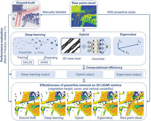
Figure 1. Workflow for evaluating the performance, effectiveness, and computational efficiency of powerline noise removal from 25 LiDAR metrics capturing vegetation height, vegetation cover, and vertical variability of vegetation. Note that the PointCNN model (applied in the deep learning and hybrid method) uses independent datasets for training and prediction. The accuracy of the three powerline extraction methods is tested with manually labeled ground truth data (performance evaluation).

2. Materials and methods

2.1 Study areas

We selected 10 study areas (500 m × 500 m per area) in the Netherlands (Figure 2(a)) for assessing powerline noise removal. We chose those areas to represent (1) powerlines in each scene, (2) sites that are spread across the country (Figure 2(a)), (3) landscapes with different canopy heights and vegetation openness (Figure 2(b)), and (4) variation in landcover types and other vegetation and powerline characteristics (Table 1). The total number of LiDAR points per area varied between 2.7 and 5.7 million (Table 1). Powerlines were present in each study area, partially overlapping with vegetation (Figure 2(a)), and the number of powerline pixels (i.e. powerlines being present at 10 × 10 m resolution) varied from 237 to 698 across the 10 study areas (Table 1). Powerline points were not separated from vegetation points in the pre-classification of the raw LiDAR point clouds, resulting in abnormal vegetation height estimates (e.g. Z values >50 m, Table 1).

Figure 2. Locations and characteristics of the 10 study areas (A‒J) in the Netherlands. (a) Spatial distribution and LiDAR point cloud visualization (colored by normalized Z values) of each study area. (b) Canopy height and landscape openness of each study area characterized by two 10-m resolution LiDAR metrics (95^th percentile of vegetation height and pulse penetration ratio, respectively). These metrics were generated from manually labeled point clouds (see detailed description in section 2.2).

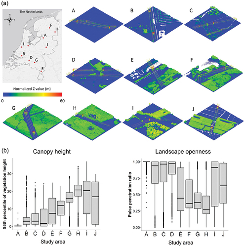
Table 1. Detailed characteristics of 10 study areas (A‒J) in the Netherlands×.

Characteristics*	Derived from	A	B	C	D	E	F	G	H	I	J
Size (ha)	Pixels	25	25	25	25	25	25	25	25	25	25
Range of raw Z value (m)	Points	−1‒46	−2‒57	−3‒54	23‒80	10‒72	10‒56	14‒76	19‒81	7‒56	−2‒52
Range of normalized Z value (m)	Points	0‒43	0‒58	0‒55	0‒52	0‒61	0‒44	0‒60	0‒59	0‒47	0‒54
Height range of powerline (m)	Points	11‒43	15‒54	16‒51	8‒50	15‒59	10‒42	13‒58	14‒55	8‒46	13‒54
Height range of vegetation (m)	Points	0‒5	0‒32	0‒28	0‒25	0‒26	0‒26	0‒33	0‒38	0‒41	0‒32
Number of powerline points	Points	47,381	16,777	20,693	78,545	28,008	23,541	22,874	19,782	16,171	15,999
Number of total points	Points	3,303,321	2,652,288	3,475,929	5,339,845	4,948,259	5,270,261	4,664,596	5,797,241	4,531,694	5,682,735
Point density (points/m^2)	Points	13.1	11.1	14.0	20.9	21.2	23.2	18.5	23.0	18.1	23.5
Mean of 95^th percentile of vegetation height	Pixels	0.28	3.98	4.67	5.48	8.75	10.39	15.05	19.93	17.27	13.65
Mean of pulse penetration ratio	Pixels	0.98	0.80	0.80	0.83	0.54	0.48	0.43	0.40	0.70	0.65
Number of powerline pixels	Pixels	442	284	370	698	283	247	334	237	288	251
Main landcover types	Visual inspection	Grassland	Bare land, buildings, vegetation patches	Road, buildings, vegetation patches	Buildings, vegetation patches,	Industrial buildings, vegetation patches	Forest, water, road	Forest, road	Forest, road	Forest, road	Forest, grassland

*Size (ha) represents 500 m × 500 m study areas. The range of raw Z values, the number of total points, and the point density were derived from raw LiDAR point clouds (AHN3). The range of normalized Z values, the height range of powerlines, the height range of vegetation, and the number of powerline points were calculated from manually labeled point clouds (ground truth). The mean values of two LiDAR metrics (95^th percentile of vegetation height and pulse penetration ratio, respectively) and the number of powerline pixels were calculated from pixels at 10 × 10 m resolution (derived from manually labeled point clouds). Landcover types were interpreted through visual inspection of the point clouds.

2.2 LiDAR data preparation

We used the pre-processed raw point clouds from airborne LiDAR as input into our workflow (Figure 1). These were collected during the third national ALS campaign of the Netherlands (AHN3, Actueel Hoogtebestand Nederland). The campaign was conducted between 2014 and 2019 in the leaf-off season covering the whole Netherlands (~34,000 km²). Raw point clouds are available from the AHN-viewer (https://www.ahn.nl/ahn-viewer). The average point density of AHN3 is 10‒16 points/m² with an overall vertical accuracy of 5 cm. Information stored for each point contains X, Y, Z, intensity, return number, number of returns, classification, scan angle rank, source ID, and GPS timestamp. The country-wide AHN3 data were pre-processed and delivered by “Rijkswaterstaat” (the Dutch Ministry of Infrastructure and Water Management), providing the pre-classification code for each point: unclassified (1), ground (2), building (6), water (9), and others (26). In the raw point cloud, points belonging to powerlines and vegetation are all defined as unclassified (1). We created digital terrain models (DTMs) at 1 m resolution and normalized the point clouds using the LAStools software (version 210,720, rapidlasso GmbH, https://rapidlasso.com/LAStools/) for each study area.

We manually labeled every point in the raw point clouds of the 10 study areas (approximately 45 million points in total) into six categories: vegetation (1), ground (2), buildings (6), water (9), powerline (14), and others (26) (e.g. bridges, cars). This was done using the ArcGIS Pro interactive editing tool for LAS classification (see https://pro.arcgis.com/en/pro-app/latest/help/data/las-dataset/interactive-las-class-code-editing.htm). The manually labeled point clouds were then used as ground truth (Figure 1), especially to (1) characterize the powerlines and vegetation in each study area (section 2.1), (2) evaluate the performance of powerline removal methods at the point level (section 2.4), and (3) generate LiDAR-derived vegetation metrics at 10 m resolution for assessing the effectiveness of the powerline extraction methods (section 2.5).

2.3 Methods for powerline extraction

We tested two point-based methods and one hybrid method for extracting powerlines. The first point-based method (deep learning method) introduces a convolutional neural network (CNN) approach to feature learning from well-labeled point clouds and classifies the target point clouds into different classes (e.g. powerlines, vegetation, and buildings). The second point-based method (eigenvalue method) uses eigenvalue decomposition of point clouds and labels the linearly distributed points as powerlines. The third method (hybrid method) was developed here and employs a 10-m resolution GeoTIFF layer of vegetation height to subset potential candidate powerline points from the original point clouds and then uses the trained CNN algorithm to classify the candidate powerline points into defined classes.

2.3.1 Point-based method using deep learning

The PointCNN proposed by Li et al. (2018) is a deep learning generalization of CNNs which shares the design of hierarchical convolution on 2D CNNs (grid-based) and generalizes it to 3D point clouds. The core $\chi$-Conv operator implemented in PointCNN is recursively applied to aggregate information from neighboring points into a subset of representative points assigning featured information (Li et al. 2018). While the output features are defined by the local (relative) coordinates of neighboring points and their associated features, they are also weighted and permuted by the $\chi$-transformation which is jointly learned across all neighborhoods. In this way, PointCNN is also capable of handling point clouds with or without additional features in a robust and uniform fashion (Li et al. 2018).

We employed the Dayton Annotated Laser Earth Scan (DALES) dataset (from Canada) to train the PointCNN model and applied the trained model to the AHN3 dataset (from the Netherlands) for prediction (Figure 1). This approach provided a robust validation for testing spatial transferability (from Canada to the Netherlands) using a point cloud dataset for prediction that is independent of the training dataset and has different characteristics (e.g. different point density and other sensor type). The DALES dataset that we used for training is a large annotated point cloud dataset, which serves as an important benchmark for evaluating deep learning algorithms applied to 3D point clouds (Varney, Asari, and Graehling 2020). It consists of more than 500 million hand-labeled point clouds obtained from ALS across multiple landscape types in British Columbia, Canada, and is currently the most extensive annotated aerial point cloud dataset that is publicly available (Varney, Asari, and Graehling 2020). The DALES dataset is delivered with separate training and testing tiles (40 tiles in total) with roughly a 70/30 percentage (i.e. 29 tiles for training and 11 tiles for testing). The training and testing scenes have a similar distribution across all labeled categories and come with a minimum and an average point density of 20 points/m² and 50 points/m², respectively. There are eight classification categories in the dataset: ground (1), vegetation (2), cars (3), trucks (4), powerlines (5), fences (6), poles (7), and buildings (8).

We first trained the PointCNN model using 29 selected DALES training tiles and validated the model using the remaining 11 DALES testing tiles. During training, we set the number of epoch to 20, and selected the model with the highest accuracy for prediction ($F1$ score of 88% for classifying the powerline category based on an evaluation with the DALES testing tiles). We then used the trained PointCNN model to predict the class of each point from the 10 study areas (AHN3 dataset) into the abovementioned eight classification categories. We chose to train the model with the most common attributes of the point cloud (i.e. X, Y, and Z values) to prevent introducing unstandardized attributes (e.g. unnormalized intensity or RGB values) into the training and prediction. We performed PointCNN model training and prediction using the deep learning framework and arcgis.learn module within a Jupyter environment. General information on the PointCNN architecture and its implementation are also available from GitHub (https://github.com/yangyanli/PointCNN).

2.3.2 Point-based method using eigenvalue decomposition

The eigenvalue method (Figure 1) identifies clusters of points that are linearly distributed based on the three eigenvalues of each individual point using the k-nearest neighbor method (Limberger and Oliveira 2015). Linear objects (e.g. powerlines) can then be segmented based on the criterion that one principal value is significantly greater than the other two principal values,

(1) ${\lambda }_3>th\ast {\lambda }_{2}AND{\lambda }_3>th\ast {\lambda }_1$(1)

where ${\lambda }_1$, ${\lambda }_2$, ${\lambda }_3$ indicate the eigenvalues calculated for each point in ascending order and $th$ is a given threshold value (Limberger and Oliveira 2015). We performed the eigenvalue calculation using the function segment_shapes() provided in the lidR package (Roussel et al. 2020). Given the point density of AHN3 (average 10‒16 points/m²) and the distribution pattern of powerline points, we set the threshold value (i.e. parameter $th$) varying from 4 to 20, and the number of neighboring points involved in the calculation (i.e. parameter $k$) varying from 6 to 40. Each combination of the parameters was tested, and the combination with the highest powerline detection rate was eventually selected as the final setting for each study area. A new attribute (“powerline”) was then added to each point, indicating the segmentation result (powerline points = 1, others = 0).

2.3.3 Hybrid method

The hybrid method combined a 2D raster layer with the PointCNN model (Figure 1). In this method, a subset of the raw point clouds (candidate points) – based on intersecting a 2D grid height layer – was first selected and then used as input into the trained PointCNN model for powerline extraction. This should increase the computational efficiency while keeping extraction accuracy comparable to the deep learning method. We used the LiDAR metric 95^th percentile of vegetation height (Hp95) derived from the raw AHN3 point clouds at a resolution of 10 m to generate a 2D mask for segmenting the candidate points. We chose Hp95 = 10 m as the height threshold for generating a binary mask because European regulations require to ensure at least 7‒10 m clearance beneath powerlines (Zhu and Hyyppä 2014). This suggests that high voltage powerlines should be >10 m high. This binary mask was then used to extract the subset of points for each study area. We then employed the trained PointCNN model (see section 2.3.1) to classify the candidate points into the same eight categories as classified in the DALES dataset. Similar to the deep learning method, we only used the X, Y, and Z values as input attributes for the prediction.

2.4 Performance of powerline extraction methods

To test H1, we evaluated the performance of the three powerline extraction methods by calculating four accuracy measures (i.e. recall, precision, quality, and $F1$ score). Recall ($Re$) is a measure of completeness or quantity of correctly extracted powerline points. Precision ($Pr$) measures the exactness or quality of correctly extracted powerline points. Quality ($Qu$) gives an overall evaluation of the completeness and exactness of powerline extraction, and the $F1$ score gives the harmonic mean of $Re$ and $Pr$ (Yang and Kang 2018). These measures were calculated as

(2) $Re=\hspace{0.17em}\frac{TP}{TP+FN}$(2)

(3) $Pr=\frac{TP}{TP+FP}$(3)

(4) $Qu=\frac{TP}{TP+FP+FN}$(4)

(5) $F1=\frac{2\ast Pr\ast Re}{Pr+Re}$(5)

where $TP$ is the amount of powerline points that are correctly identified as powerlines, $FN$ is the amount of powerline points that are misidentified as others, and $FP$ is the amount of other points that are misidentified as powerlines. The manually labeled points were used as ground truth to assess correct (true) or incorrect (false) classifications. Each accuracy measure was calculated for each study area (n = 10) and compared with the average canopy height of each study area. Note that the accuracy calculations were done without the transmission towers (i.e. powerline points only) because (1) the eigenvalue method is only designed to identify linear objects (i.e. powerlines) and (2) the shape of transmission towers differs between the training dataset (DALES from Canada) and the prediction dataset (AHN3 from the Netherlands) for the PointCNN model.

2.5 Effectiveness of powerline removal on LiDAR metrics

To test H2, we analyzed the effectiveness of powerline removal for 25 LiDAR metrics representing different aspects of vegetation height (7 metrics), vegetation cover (11 metrics), and vertical variability of vegetation (7 metrics) (see details in Appendix Table A1). For each metric, we compared their values after applying the three powerline extraction methods with the values derived from ground truth (manually labeled point clouds) and raw point clouds (with powerline noise) (Figure 1). All metrics were calculated at a 10 m resolution for each study area using a recently developed high-throughput workflow “Laserfarm” for generating geospatial data products of ecosystem structure from ALS point clouds (Kissling et al. 2022). Within each study area, we assessed only the pixels with powerlines, i.e. those 10-m resolution grid cells in which powerlines occurred (n = 3434 across all study areas).

2.6 Computational efficiency of powerline extraction methods

To test H3, we evaluated the computational efficiency of the three powerline extraction methods (Figure 1). We estimated execution times for each study area using the Jupyter Notebook environment (for the deep learning and hybrid methods) and the R environment (for the eigenvalue method). This was done on a DELL XPS laptop with 2.40 GHz Intel Core i9 processor and 32 GB RAM and included loading the data, running the model/method, predicting the results and exporting the results. We further calculated the number of processed points for each method at each study area and the time efficiency (points/sec) of each method by dividing the amount of processed points by the execution time.

3. Results

3.1 Performance of powerline extraction methods

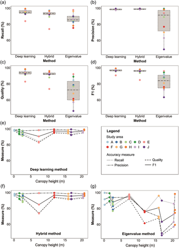
In line with our hypothesis H1, the deep learning method generally performed best in terms of accuracy (Figure 3(a–d)). It showed a high recall (94.52% ± 4.13%), precision (98.61% ± 0.72%), quality (93.27% ± 4.10%), and $F1$ score (96.47% ± 2.26%) across all 10 study areas (Figure 3(a–d), Appendix Table B1). It also removed on average about 95% of all powerline points across the study areas (94.52% ± 4.12%, see Appendix Figure B1). The hybrid method also showed a very good performance, similar to the deep learning method (Figure 3(a–d)), with an equally high precision (98.93% ± 0.50%) and $F1$ score (95.10% ± 3.61%) and a slightly lower recall (91.76% ± 6.30%) and quality (90.84% ± 6.12%) (see Appendix Table B1). The hybrid method also removed a high proportion of powerline points across the study areas (91.76% ± 6.30%, see Appendix Figure B1). The eigenvalue method generally performed poorer than the other two methods (Figure 3(a–d)), with an overall lower recall (86.58% ± 6.73%), precision (83.35% ± 16.80%), quality (71.41% ± 14.40%), and $F1$ score (82.48% ± 10.07%) (see Appendix Table B1). It also showed a lower proportion of removed powerline points than the other two methods (86.58% ± 6.73%), except in areas E and G where it removed more points (see Appendix Figure B1). Moreover, the eigenvalue method showed a distinct decrease in precision, quality and $F1$ score in landscapes with tall canopies (areas F–J) compared to areas with low vegetation (areas A–E) (Figure 3(g)). In contrast, the deep learning and hybrid methods retained high accuracies in all study areas (Figure 3e and 3f), supporting the expectation of a good performance in areas with different landscape characteristics (H1). The only exception was study area E, where the eigenvalue method outperformed the other two methods in recall, quality, and $F1$ score (Figure 3(e–g)).

Figure 3. Performance evaluation of powerline extraction methods. Accuracy of three methods (i.e. deep learning, hybrid, and eigenvalue method) as quantified by (a) recall, (b) precision, (c) quality, and (d) $F$1 score. All four accuracy measures together along a gradient of canopy height, shown separately for (e) deep learning, (f) hybrid, and (g) eigenvalue method. Dots with different colors indicate the 10 different study areas (A‒J). Different line types indicate the different accuracy measures (recall, precision, quality, and $F$1 score).

3.2 Effectiveness of powerline removal on LiDAR metrics

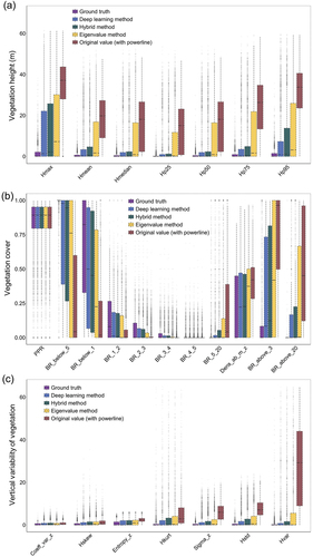
Most of the 25 LiDAR metrics were improved after removing powerline noise (Figure 4). Especially for vegetation height (in line with H2), metrics improved substantially through the removal of abnormal Z values from raw cloud points (with powerline noise) by the deep learning and hybrid method, respectively (Figure 4(a)). For vegetation cover, the effectiveness of powerline extraction methods differed among LiDAR metrics (Figure 4(b)). For instance, effectiveness was high for metrics capturing the density of vegetation points below 1 m or below 5 m (Figure 4(b)), supporting the idea that powerline points can strongly bias vegetation cover in the lower strata (H2). Effectiveness was also high for metrics capturing vegetation cover in the upper layer (e.g. the density of vegetation points within 5–20 m, above 3 m, or above 20 m, Figure 4(b)), but low for metrics capturing vegetation cover in the middle layer (e.g. within 3–4 m and 4–5 m, Figure 4(b)). Finally, the effectiveness of powerline extraction methods was much less pronounced on metrics representing the vertical variability of vegetation, except for the variance of vegetation height (Hvar) (Figure 4(c)).

Figure 4. Effectiveness of powerline removal on 25 LiDAR metrics of ecosystem structure. Metrics after powerline removal (using the deep learning, hybrid, and eigenvalue method, respectively) are compared to metrics generated from ground truth (i.e. manually labeled point clouds) and metrics derived from the raw point clouds (i.e. with powerline noise). The metrics represent vegetation height (7 metrics), vegetation cover (11 metrics), and vertical variability of vegetation (7 metrics). See Appendix Table A1 for metric abbreviations. Box-and-whisker plots show the values of each metric calculated for pixels with powerlines (n = 3434) across the 10 study areas. Boxes show the median and interquartile range, with whiskers (stippled lines) extending to 1.5 times the interquartile range and dots beyond.

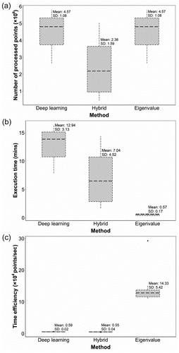
3.3 Computational efficiency of powerline extraction methods

In line with hypothesis H3, the computational efficiency of the deep learning method was low because of the large number of points to be processed (Figure 5(a)), the long execution time (Figure 5(b)), and its low time efficiency (Figure 5(c)). In contrast, the eigenvalue method was the most time-efficient method (Figure 5(c)), having a more than 20 times faster execution time than the deep learning method (Figure 5(b)). With larger data volumes and a higher number of processed points, the execution time of both the deep learning and hybrid methods strongly increased (Appendix Table B2). However, compared to the deep learning method, the hybrid method reduced the total number of processed points by almost 50% (Appendix Table B2). This resulted in a substantial reduction of the execution time (Figure 5(b)), supporting our initial expectation (H3). Compared to the deep learning method, the execution time reduction of the hybrid method ranged from 11% (in area G, densely vegetated landscape with tall canopy height) to 80% (in area C, open landscape with low canopy height) (Appendix Table B2).

Figure 5. Computational efficiency of three powerline extraction methods (i.e. deep learning, hybrid, and eigenvalue method) explained by (a) number of processed points, (b) execution time, and (c) time efficiency. Boxes show the median and interquartile range, with whiskers (stippled lines) extending to 1.5 times the interquartile range and dots beyond. The mean and standard deviation are given next to each boxplot.

4. Discussion

We evaluated the performance, effectiveness, and computational efficiency of three powerline removal methods for improving 25 LiDAR metrics of ecosystem structure derived from ALS point clouds. The deep learning and hybrid methods (based on the PointCNN model) provided a consistently high accuracy of powerline noise removal across study areas with different canopy heights and landscape openness, whereas the eigenvalue method had a poorer performance, but a higher time efficiency. Powerline removal was most effective in LiDAR metrics representing vegetation height as well as vegetation cover in low and upper vegetation layers. We further showed that the hybrid method can greatly reduce the execution time compared to the deep learning method, making it a computational-efficient and accurate method for upscaling powerline removal to multi-terabyte ALS datasets at a national extent.

Deep learning is rapidly transforming the fields of Earth science (Reichstein et al. 2019) and ecology (Borowiec et al. 2022), and our results confirm the high potential of deep learning applications for point cloud classification (Bello et al. 2020; Guo et al. 2021; Wen et al. 2021). By removing ~95% of the powerline points from the raw point clouds, the applied deep learning method (i.e. PointCNN) was highly successful, with an average accuracy of ~96% (across the four accuracy measures, i.e. recall, precision, quality, and $F1$ score). The impressive performance of the PointCNN was even achieved using an independent test by training the model with a dataset from North America (i.e. Canada) and applying it to a dataset from Europe (i.e. the Netherlands), which has different characteristics (e.g. lower point density and other sensor types). The high accuracy of the PointCNN model is similar to the accuracy of other deep learning methods, e.g. the KPConv model proposed by Thomas et al. (2019) and methods tested with UAV-based LiDAR datasets (Chen et al. 2022). Due to the linear and narrow attributes of powerlines, relatively high point densities are usually needed to achieve good results in powerline extraction (Matikainen et al. 2016). In our study, we obtained an average $F1$ score of 96.5% with a point density of 10‒16 points/m² (AHN3 dataset). Lower point densities (e.g. 4–7 points/m²) can result in a reduced performance of deep learning methods for 3D point classification, e.g. an average $F1$ score of 61.5% when the PointCNN method is applied to the ISPRS benchmark dataset (Wen et al. 2021). On the other hand, deep learning methods applied to point clouds with higher point densities (e.g. >20 points/m²) typically show good performance of powerline extraction, e.g. an average $F1$ score of 97.1% when the DCPLD-Net method is applied to four datasets varying in point density from 22 to 120 points/m² (Chen, Lin, and Liao 2022). We therefore expect that deep learning methods for powerline extraction show good performance with ALS datasets that have point densities of 10‒20 points/m² or above.

Compared to deep learning, the hybrid method also showed a high overall accuracy (average 94%), but a remarkable decrease in execution time. Other applications of hybrid methods also demonstrate a similar performance, such as the one proposed by Zhu and Hyyppä (2014), which successfully classified 93% of powerline points from forested areas in Finland. This encourages the use of hybrid methods due to their high accuracy and simultaneously a reduced execution time. In contrast, the eigenvalue method generally performed poorer than the deep learning and the hybrid methods, except in relatively open landscapes with low vegetation (e.g. our study areas A‒C). While eigenvalue methods can successfully remove a large number of powerline points in certain situations (e.g. McLaughlin 2006), they also require additional parameter adjustments for optimization in different settings (e.g. different landscapes where powerlines occur or different characteristics of powerlines). This impairs their generalizability (Chen et al. 2022) for accurately detecting powerlines in different landscapes (e.g. Jwa and Sohn 2012; Nardinocchi, Balsi, and Esposito 2020) and hence limits the application of eigenvalue methods for upscaling to large areas with heterogeneous landscapes.

Our results show that the effectiveness of powerline removal depends on which properties of the ecosystem structure are captured (i.e. vegetation height, cover, or vertical variability) and in which stratum (e.g. low, middle, or upper layer). For instance, vegetation height metrics were more strongly improved than other metrics after removing the abnormally large Z values from the powerlines. Metrics capturing the density of low vegetation (e.g. below 1 m) and upper vegetation (e.g. canopy cover above 20 m) also showed strong improvements after powerline removal, especially when compared to other vegetation cover metrics such as vegetation density of the middle layer (e.g. between 3–4 m and 4–5 m). Airborne laser scanning often has difficulties in capturing low vegetation when canopies are dense, suggesting that low strata with few vegetation points (e.g. below 1 m) are more prone to misclassifications (Assmann et al. 2022). When powerline points (usually above 10 m) are identified and removed from vegetation points in the upper vegetation layer, the calculation of vegetation cover below 1 m or above 20 m can be greatly improved. In contrast, the effect of powerline removal on vegetation cover within 4–5 m and on the pulse penetration ratio was almost neglectable. Overall, our results can provide guidance on which LiDAR metrics of the 3D ecosystem structure might be most biased if powerlines are present.

Upscaling powerline extraction to a national, multi-terabyte ALS dataset requires time efficient and highly accurate methods. In the Netherlands, there are approximately 24,500 km overhead high-voltage powerlines with 110‒380 kV (grid map available at: https://data.rivm.nl/apps/netkaart/). For the three tested methods, the hybrid method was the most promising candidate for upscaling because it is highly accurate across different landscapes and simultaneously reduces the computation time compared to the deep learning method. Note that the application stage of the deep learning method is already much more efficient than in its training stage: the training stage of the deep learning method costs on average 14 h per epoch (around 100 h in total for training on 350 million points), while in the application stage, it predicts (on average) 4.5 million points in 13 mins (see Appendix Table B2). Considering the total amount of points of the Dutch AHN3 data (~700 billion points) covering the whole Netherlands (~34,000 km²) (Kissling et al. 2023), we estimate that the hybrid method would require to process ~30 billion points when considering only the candidate powerline points after subsetting (i.e. applying a 10-m resolution binary mask with the 95^th percentile of vegetation height >10 m). The estimated CPU time for the hybrid method (~63 days) is about 5% of the time for the deep learning method applied to the whole country (~1373 days), and thus only slightly more than the eigenvalue method (~56 days). These estimated execution times are based on a single process local machine. When upscaling the process to a high-performance computing (HPC) or cloud environment, the execution time could be strongly shortened by parallelization and distributed processing with the benefit of multi-core CPU or multi-node GPU clusters (Kissling et al. 2022). For instance, the actual execution wall-time can be reduced to ~3 days when using a cluster of 10 virtual machines that each has two cores.

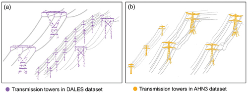
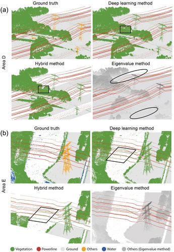
Some small biases and misclassifications will remain, independent of the applied powerline extraction method (Figure 6). The eigenvalue method failed to identify powerline points with a discontinuous distribution, i.e. when large gaps between neighboring powerline points occurred (Figure 6(a)). Both the deep learning and hybrid methods showed similar misclassifications, e.g. in areas where powerlines crossed water (Figure 6(b)). This probably stems from the input training data (DALES dataset) that has no powerlines above water (Varney, Asari, and Graehling 2020), resulting in misclassifications in the prediction. A general challenge for the classification was the lack of identification of transmission towers (Otcenasova, Hoger, and Altus 2014) (Figure 6). Only very few transmission towers are included in the training dataset (DALES dataset) and the shape of transmission towers differs between Canada and the Netherlands (see Appendix Figure C1). A future solution could be to collect more training samples to capture various shapes of transmission towers, which then can improve the capability of the PointCNN model to identify them.

Figure 6. Examples of misclassifications from powerline extraction methods in comparison with ground truth. (a) Examples of misclassifications in study area D when powerlines are close to tree crowns (deep learning and hybrid method) or when gaps between powerline points are relatively large (eigenvalue method). (b) Examples of misclassifications in study area E for powerlines above water (deep learning and hybrid method, but not eigenvalue method). Note that transmission towers were generally not correctly classified. For visualization purposes, the eight categories classified by the deep learning and hybrid methods were grouped into four classes: ground, vegetation, powerlines, water and others (including buildings, etc.). For the eigenvalue method, the result only contained two classes: powerline and others.

5. Conclusion

Country-wide airborne LiDAR data provide great opportunities for generating high-quality metrics of ecosystem structure across large spatial extents. However, powerlines can introduce biases and noises into LiDAR metrics of vegetation height, cover, and vertical variability. We show that deep learning models in combination with grid-based approaches can provide high accuracy and simultaneously reduce execution times compared to the deep learning method. This makes the hybrid methods a computational-efficient and accurate approach for upscaling powerline removal to a national extent. Although the eigenvalue method generally performed poorer than the deep learning and the hybrid methods, it can still achieve high accuracy in relatively open landscapes with low vegetation. Powerline removal methods can largely remove abnormal Z values, especially for LiDAR metrics that capture vegetation height and vegetation cover in low and upper vegetation layers. Developing upscaling solutions on high-performance computing or cloud environments together with additional training data will be crucial next steps for generating high-quality metrics of ecosystem structure at regional or national extents.

Acknowledgments

We thank three reviewers and the handling editor for constructive comments. We acknowledge the effort of the development team of the “Laserfarm” workflow from Netherlands eScience Center, through the “eEcoLiDAR” project (Kissling et al. 2017), namely Christiaan Meijer, Ou Ku, Francesco Nattino, and Meiert W. Grootes. We also acknowledge the support from LifeWatch (https://www.lifewatch.eu/) for the further development and exploration of our tools in a virtual research environment. W.D.K. acknowledges support from the European Commission (grant agreement No 101060639) for the Horizon Europe research and innovation action MAMBO (Modern Approaches to the Monitoring of BiOdiversity).

Disclosure statement

No potential conflict of interest was reported by the author(s).

Data availability statement

The raw point clouds (AHN3) and the manually labeled point clouds (ground truth) for the study areas, the code for implementing the powerline extraction methods, and the 25 LiDAR metrics generated from different input data (i.e. raw point cloud, ground truth, deep learning method, hybrid method, and eigenvalue method) are available from Zenodo (https://doi.org/10.5281/zenodo.7701809). The notebook about powerline extraction using the deep learning method (PointCNN model) is available from GitHub (https://github.com/ShiYifang/Powerline_extraction). The country-wide Dutch AHN3 data are available from https://app.pdok.nl/rws/ahn3/download-page/. The DALES dataset can be accessed via https://udayton.edu/engineering/research/centers/vision_lab/research/was_data_analysis_and_processing/dale.php.

Appendices Appendix A

Table A1. Twenty-five LiDAR metrics representing vegetation height, vegetation cover, and vertical variability of vegetation. Additional information on the ecological meaning of the metrics can be found in Kissling et al. (2023).

Abbreviation	LiDAR metrics	Description
Vegetation height
Hmax	Maximum vegetation height	Maximum value of normalized Z within a grid cell
Hmean	Mean vegetation height	Mean value of normalized Z within a grid cell
Hmedian	Median vegetation height	Median value of normalized Z within a grid cell
Hp25	25^th percentile of vegetation height	The 25^th percentile of normalized Z values within a grid cell
Hp50	50^th percentile of vegetation height	The 50^th percentile of normalized Z values within a grid cell
Hp75	75^th percentile of vegetation height	The 75^th percentile of normalized Z values within a grid cell
Hp95	95^th percentile of vegetation height	The 95^th percentile of normalized Z values within a grid cell
Vegetation cover
PPR	Pulse penetration ratio	Ratio of the number of ground points to the total number of points within a grid cell
BR_below_5	Density of vegetation below 5 m	Ratio of the number of vegetation points below 5 m to the total number of vegetation points within a grid cell
BR_below_1	Density of vegetation below 1 m	Ratio of the number of vegetation points below 1 m to the total number of vegetation points within a grid cell
BR_1_2	Density of vegetation within 1‒2 m	Ratio of the number of vegetation points within 1‒2 m to the total number of vegetation points within a grid cell
BR_2_3	Density of vegetation within 2‒3 m	Ratio of the number of vegetation points within 2‒3 m to the total number of vegetation points within a grid cell
BR_3_4	Density of vegetation within 3‒4 m	Ratio of the number of vegetation points within 3‒4 m to the total number of vegetation points within a grid cell
BR_4_5	Density of vegetation within 4‒5 m	Ratio of the number of vegetation points within 4‒5 m to the total number of vegetation points within a grid cell
BR_5_20	Density of vegetation within 5‒20 m	Ratio of the number of vegetation points within 5‒20 m to the total number of vegetation points within a grid cell
Dens_ab_m_z	Density of vegetation above mean height	Ratio of the number of vegetation points above mean height to the total number of vegetation points within a grid cell
BR_above_3	Density of vegetation above 3 m	Ratio of the number of vegetation points above 3 m to the total number of vegetation points within a grid cell
BR_above_20	Density of vegetation above 20 m	Ratio of the number of vegetation points above 20 m to the total number of vegetation points within a grid cell
Vertical variability of vegetation
Coeff_var_z	Coefficient of variation (CV)	CV of normalized Z values within a grid cell
Hskew	Skewness of vertical vegetation distribution	Skewness of normalized Z values within a grid cell
Entropy_z	Shannon index (foliage height diversity)	The negative sum of the proportion of points within .5 m height layers multiplied with the logarithm of the proportion of points within .5 m height layers within a grid cell
Hkurt	Kurtosis of vertical vegetation distribution	Kurtosis of normalized Z values within a grid cell
Sigma_z	Roughness of vegetation	Residual standard deviation of a locally fitted plane within a cylinder
Hstd	Standard deviation (SD) of vegetation height	SD of normalized Z values within a grid cell
Hvar	Variance of vertical vegetation distribution	Variance of normalized Z values within a grid cell

Appendix B

Table B1. Performance of three the powerline extraction methods (deep learning, hybrid, eigenvalue decomposition) in each study area (A‒J). Four accuracy measures are provided, namely the recall ($Re$), precision ($Pr$), quality ($Qu$), and $F1$ score. The mean (Mean) and standard deviation (SD) are calculated across the ten study areas (A‒J).

Study area	Deep learning				Hybrid				Eigenvalue decomposition
	$Re$	$Pr$	$Qu$	$F1$	$Re$	$Pr$	$Qu$	$F1$	$Re$	$Pr$	$Qu$	$F1$
A	98.75	98.88	97.65	98.81	97.5	98.54	96.11	98.02	84.79	99.77	84.63	91.67
B	94.57	97.72	92.52	96.12	94.33	98.52	93.01	96.38	82.93	93.85	78.65	88.05
C	93.38	97.56	91.25	95.42	89.33	98.36	88.02	93.63	84.91	89.13	76.94	86.97
D	83.89	98.49	82.82	90.6	74.04	99.38	73.7	84.86	97.79	94.09	92.13	95.9
E	94.13	99.09	93.32	96.55	92.41	99.24	91.76	95.7	89.61	99.25	89.01	94.19
F	95.45	99.49	94.98	97.42	94.15	99.64	93.83	96.82	75.41	77.03	61.57	76.21
G	95.41	98.78	94.29	97.06	92.77	98.54	91.51	95.57	96.11	69.98	68.05	80.99
H	99.36	99.01	98.39	99.19	96.53	99.23	95.82	97.87	78.17	98.37	59.53	74.63
I	97.59	97.54	95.24	97.56	94.6	98.29	93.06	96.4	86.07	63.05	57.21	72.78
J	92.67	99.54	92.28	95.98	91.96	99.6	91.62	95.63	90.01	48.94	46.42	63.41
Mean	94.52	98.61	93.27	96.47	91.76	98.93	90.84	95.10	86.58	83.35	71.41	82.48
SD	4.13	0.72	4.10	2.26	6.30	0.50	6.12	3.61	6.73	16.80	14.40	10.07

Figure B1. Violin plot of the proportion of removed powerline points across 10 study areas using three powerline extraction methods (deep learning, hybrid, and eigenvalue method). The proportion of remaining powerline points from each tested method was calculated relative to the total amount of manually labeled powerline points (ground truth).

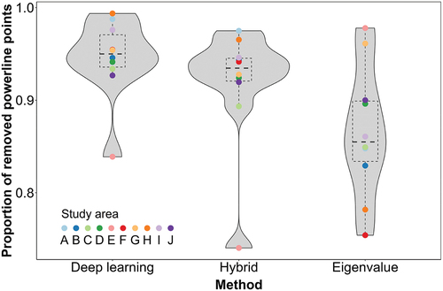
Table B2. Computational efficiency of three powerline extraction methods (deep learning, hybrid, and eigenvalue) in 10 study areas (A‒J). Summarized are the number of processed points, the executing times, and the time efficiency for each method*. The deep learning and eigenvalue methods have the same number of processed points because both of them consider the whole point clouds as input, while the hybrid method only uses the candidate points (i.e. subsets of the whole point clouds).

Study area	Data volume (MB)	Number of processed points			Execution time (min)			Time efficiency (points/sec)
		Deep learning	Hybrid	Eigenvalue	Deep learning	Hybrid	Eigenvalue	Deep learning	Hybrid	Eigenvalue
A	88.2	3,303,321	678,731	3,303,321	8.4	2.0	0.5	6593	5628	112358
B	70.8	2,652,288	457,185	2,652,288	7.8	1.7	0.3	5660	4482	138140
C	92.8	3,475,929	589,571	3,475,929	10.1	2.0	0.4	5725	4963	152453
D	142	5,339,845	2,312,700	5,339,845	14.7	6.9	0.8	6062	5627	112655
E	132	4,948,259	2,072,722	4,948,259	14.1	6.2	0.7	5841	5617	124956
F	140	5,270,261	1,797,204	5,270,261	15.3	5.5	0.7	5737	5496	129173
G	124	4,664,596	4,101,100	4,664,596	13.7	12.1	0.6	5695	5640	127448
H	154	5,797,241	5,033,447	5,797,241	16.2	14.4	0.3	5950	5838	292790
I	121	4,531,694	2,806,415	4,531,694	12.7	8.2	0.7	5942	5704	107897
J	151	5,682,735	3,923,754	5,682,735	16.4	11.6	0.7	5793	5652	135303
Total	1215.8	45,666,169	23,772,829	45,666,169	129.3	70.4	5.7	5885	5628	134470
Mean	121.6	4566616.9	2377282.9	4566616.9	12.9	7.0	0.6	5899.9	5464.7	143317.4
SD	28.5	1078053.5	1591772.9	1078053.5	3.1	4.5	0.2	275.5	415.9	54220.6

*The experiment was performed on a DELL XPS laptop with 2.40 GHz Intel Core i9 processor and 32 GB RAM.

Appendix C

Figure C1. Variation in the shapes of transmission towers as captured in different airborne laser scanning datasets. (a) Transmission towers in Canada (DALES dataset) which were used for training the deep learning model. (b) Transmission towers in the Netherlands (AHN3 dataset) which were used for prediction.

References

- Almeida, D. R. A. D., E. N. Broadbent, M. P. Ferreira, P. Meli, A. M. A. Zambrano, E. B. Gorgens, A. F. Resende, et al. 2021. “Monitoring Restored Tropical Forest Diversity and Structure Through UAV-Borne Hyperspectral and Lidar Fusion.” Remote Sensing of Environment 264:112582. https://doi.org/10.1016/j.rse.2021.112582.
- Asner, G. P., C. B. Anderson, R. E. Martin, D. E. Knapp, R. Tupayachi, F. Sinca, and Y. Malhi. 2014. “Landscape-Scale Changes in Forest Structure and Functional Traits Along an Andes-To-Amazon Elevation Gradient.” Biogeosciences 11 (3): 843–20. https://doi.org/10.5194/bg-11-843-2014.
- ASPRS. 2019. “LAS Specification 1.4-R15.” In ASPRS the Imaging & Geospatial Information Society, 50. MD, USA: American Society for Photogrammetry & Remote Sensing .
- Assmann, J. J., J. E. Moeslund, U. A. Treier, and S. Normand. 2022. “EcoDes-DK15: High-Resolution Ecological Descriptors of Vegetation and Terrain Derived from Denmark’s National Airborne Laser Scanning Data Set.” Earth System Science Data 14 (2): 823–844. https://doi.org/10.5194/essd-14-823-2022.
- Awrangjeb, M. 2019. “Extraction of Power Line Pylons and Wires Using Airborne LiDar Data at Different Height Levels.” Remote Sensing 11 (15): 1798. https://doi.org/10.3390/rs11151798.
- Bello, S. A., Y. Shangshu, C. Wang, J. M. Adam, and J. Li. 2020. “Review: Deep Learning on 3D Point Clouds.” Remote Sensing 12 (11): 1729. https://doi.org/10.3390/rs12111729.
- Borowiec, M. L., R. B. Dikow, P. B. Frandsen, A. McKeeken, G. Valentini, and A. E. White. 2022. “Deep Learning as a Tool for Ecology and Evolution.” Methods in Ecology and Evolution 13 (8): 1640–1660. https://doi.org/10.1111/2041-210x.13901.
- Chen, C., A. Jin, B. Yang, R. Ma, S. Sun, Z. Wang, Z. Zong, and F. Zhang. 2022. “DCPLD-Net: A Diffusion Coupled Convolution Neural Network for Real-Time Power Transmission Lines Detection from UAV-Borne LiDar Data.” International Journal of Applied Earth Observation and Geoinformation 112:102960. https://doi.org/10.1016/j.jag.2022.102960.
- Chen, Y., J. Lin, and X. Liao. 2022. “Early Detection of Tree Encroachment in High Voltage Powerline Corridor Using Growth Model and UAV-Borne LiDar.” International Journal of Applied Earth Observation and Geoinformation 108:102740. https://doi.org/10.1016/j.jag.2022.102740.
- Deibe, D., M. Amor, and R. Doallo. 2020. “Big Data Geospatial Processing for Massive Aerial LiDar Datasets.” Remote Sensing 12 (4): 719. https://doi.org/10.3390/rs12040719.
- Eitel, J. U. H., B. Höfle, L. A. Vierling, A. Abellán, G. P. Asner, J. S. Deems, C. L. Glennie, et al. 2016. “Beyond 3-D: The New Spectrum of Lidar Applications for Earth and Ecological Sciences.” Remote Sensing of Environment 186:372–392. https://doi.org/10.1016/j.rse.2016.08.018.
- Guo, B., X. Huang, F. Zhang, and G. Sohn. 2015. “Classification of Airborne Laser Scanning Data Using JointBoost.” Isprs Journal of Photogrammetry & Remote Sensing 100:71–83. https://doi.org/10.1016/j.isprsjprs.2014.04.015.
- Guo, Q., Y. Su, T. Hu, H. Guan, S. Jin, J. Zhang, X. Zhao, et al. 2021. “Lidar Boosts 3D Ecological Observations and Modelings: A Review and Perspective.” IEEE Geoscience and Remote Sensing Magazine 9 (1): 232–257. https://doi.org/10.1109/MGRS.2020.3032713.
- Guo, Y., H. Wang, Q. Hu, H. Liu, L. Liu, and M. Bennamoun. 2021. “Deep Learning for 3D Point Clouds: A Survey.” IEEE Transactions Pattern Analysis Machine Intelligent 43 (12): 4338–4364. https://doi.org/10.1109/TPAMI.2020.3005434.
- Huang, W., K. Dolan, A. Swatantran, K. Johnson, H. Tang, J. O’Neil-Dunne, R. Dubayah, and G. Hurtt. 2019. “High-Resolution Mapping of Aboveground Biomass for Forest Carbon Monitoring System in the Tri-State Region of Maryland, Pennsylvania and Delaware, USA.” Environmental Research Letters 14 (9): 095002. https://doi.org/10.1088/1748-9326/ab2917.
- Jung, J., E. Che, M. J. Olsen, and K. C. Shafer. 2020. “Automated and Efficient Powerline Extraction from Laser Scanning Data Using a Voxel-Based Subsampling with Hierarchical Approach.” Isprs Journal of Photogrammetry & Remote Sensing 163:343–361. https://doi.org/10.1016/j.isprsjprs.2020.03.018.
- Jwa, Y., and G. Sohn. 2012. “A Piecewise Catenary Curve Model Growing for 3D Power Line Reconstruction.” Photogrammetric Engineering & Remote Sensing 78 (12): 1227–1240. https://doi.org/10.14358/pers.78.11.1227.
- Kim, H. B., and G. Sohn. 2013. “Point-Based Classification of Power Line Corridor Scene Using Random Forests.” Photogrammetric Engineering & Remote Sensing 79 (9): 821–833. https://doi.org/10.14358/pers.79.9.821.
- Kissling, W. D., A. C. Seijmonsbergen, R. P. B. Foppen, and W. Bouten. 2017. “eEcolidar, eScience Infrastructure for Ecological Applications of LiDar Point Clouds: Reconstructing the 3D Ecosystem Structure for Animals at Regional to Continental Scales.” Research Ideas and Outcomes 3. https://doi.org/10.3897/rio.3.e14939.
- Kissling, W. D., Y. Shi, Z. Koma, C. Meijer, O. Ku, F. Nattino, A. C. Seijmonsbergen, and M. W. Grootes. 2022. “Laserfarm – a High-Throughput Workflow for Generating Geospatial Data Products of Ecosystem Structure from Airborne Laser Scanning Point Clouds.” Ecological Informatics 72:101836. https://doi.org/10.1016/j.ecoinf.2022.101836.
- Kissling, W. D., Y. Shi, Z. Koma, C. Meijer, O. Ku, F. Nattino, A. C. Seijmonsbergen, and M. W. Grootes. 2023. “Country-Wide Data of Ecosystem Structure from the Third Dutch Airborne Laser Scanning Survey.” Data in Brief 46:108798. https://doi.org/10.1016/j.dib.2022.108798.
- LaRue, E. A., F. W. Wagner, S. Fei, J. W. Atkins, R. T. Fahey, C. M. Gough, and B. S. Hardiman. 2020. “Compatibility of Aerial and Terrestrial LiDar for Quantifying Forest Structural Diversity.” Remote Sensing 12 (9): 1407. https://doi.org/10.3390/rs12091407.
- Li, Y., R. Bu, M. Sun, W. Wei, X. Di, and B. Chen. 2018. “PointCnn: Convolution on χ-Transformed Points.” Advances in Neural Information Processing Systems 31:820–830. https://doi.org/10.48550/arXiv.1801.07791.
- Li, N., O. Kahler, and N. Pfeifer. 2021. “A Comparison of Deep Learning Methods for Airborne Lidar Point Clouds Classification.” IEEE Journal of Selected Topics in Applied Earth Observations & Remote Sensing 14:6467–6486. https://doi.org/10.1109/jstars.2021.3091389.
- Limberger, F. A., and M. M. Oliveira. 2015. “Real-Time Detection of Planar Regions in Unorganized Point Clouds.” Pattern Recognition 48 (6): 2043–2053. https://doi.org/10.1016/j.patcog.2014.12.020.
- Liu, K., Z. Gao, F. Lin, and B. M. Chen. 2023. “FG-Net: A Fast and Accurate Framework for Large-Scale LiDar Point Cloud Understanding.” IEEE Transactions on Cybernetics 53 (1): 553–564. https://doi.org/10.1109/TCYB.2022.3159815.
- Matikainen, L., M. Lehtomäki, E. Ahokas, J. Hyyppä, M. Karjalainen, A. Jaakkola, A. Kukko, and T. Heinonen. 2016. “Remote Sensing Methods for Power Line Corridor Surveys.” Isprs Journal of Photogrammetry & Remote Sensing 119:10–31. https://doi.org/10.1016/j.isprsjprs.2016.04.011.
- McLaughlin, R. A. 2006. “Extracting Transmission Lines from Airborne LiDar Data.” IEEE Geoscience & Remote Sensing Letters 3 (2): 222–226. https://doi.org/10.1109/lgrs.2005.863390.
- Morsy, S., A. Shaker, and A. El-Rabbany. 2022. “Classification of Multispectral Airborne LiDar Data Using Geometric and Radiometric Information.” Geomatics 2 (3): 370–389. https://doi.org/10.3390/geomatics2030021.
- Moudrý, V., A. F. Cord, L. Gábor, G. Vaglio Laurin, V. Barták, K. Gdulová, M. Malavasi, et al. 2023. “Vegetation Structure Derived from Airborne Laser Scanning to Assess Species Distribution and Habitat Suitability: The Way Forward.” Diversity & Distributions 29 (1): 39–50. https://doi.org/10.1111/ddi.13644.
- Nardinocchi, C., M. Balsi, and S. Esposito. 2020. “Fully Automatic Point Cloud Analysis for Powerline Corridor Mapping.” IEEE Transactions on Geoscience & Remote Sensing 58 (12): 8637–8648. https://doi.org/10.1109/tgrs.2020.2989470.
- Otcenasova, A., M. Hoger, and J. Altus. 2014. “Possible Use of Airborne LiDar for Monitoring of Power Lines in Slovak Republic.” Paper presented at the Proceedings of the 2014 15th International Scientific Conference on Electric Power Engineering (EPE), Brno-Bystrc, Czech Republic, May 12-14 2014.
- Peng, S., X. Xiaohuan, C. Wang, P. Dong, P. Wang, and S. Nie. 2019. “Systematic Comparison of Power Corridor Classification Methods from ALS Point Clouds.” Remote Sensing 11 (17). https://doi.org/10.3390/rs11171961.
- Potapov, P., L. Xinyuan, A. Hernandez-Serna, A. Tyukavina, M. C. Hansen, A. Kommareddy, A. Pickens, et al. 2021. “Mapping Global Forest Canopy Height Through Integration of GEDI and Landsat Data.” Remote Sensing of Environment 253:112165. https://doi.org/10.1016/j.rse.2020.112165.
- Qi, C. R., H. Su, M. Kaichun, and L. J. Guibas. 2017. “PointNet: Deep Learning on Point Sets for 3d Classification and Segmentation.” Paper presented at the Proceedings of the IEEE conference on computer vision and pattern recognition. https://doi.org/10.48550/arXiv.1612.00593.
- Qi, C. R., L. Yi, S. Hao, and L. J. Guibas. 2017. “Pointnet++: Deep Hierarchical Feature Learning on Point Sets in a Metric Space.” Advances in Neural Information Processing Systems 30. https://doi.org/10.48550/arXiv.1706.02413.
- Reichstein, M., G. Camps-Valls, B. Stevens, M. Jung, J. Denzler, N. Carvalhais, and Prabhat. 2019. “Deep Learning and Process Understanding for Data-Driven Earth System Science.” Nature 566 (7743): 195–204. https://doi.org/10.1038/s41586-019-0912-1.
- Roussel, J.-R., A. Achim, and D. Auty. 2021. “Classification of High-Voltage Power Line Structures in Low Density ALS Data Acquired Over Broad Non-Urban Areas.” Peer Journal Computer Science 7:e672. https://doi.org/10.7717/peerj-cs.672.
- Roussel, J.-R., D. Auty, N. C. Coops, P. Tompalski, T. R. H. Goodbody, A. S. Meador, J.-F. Bourdon, F. de Boissieu, and A. Achim. 2020. “lidR: An R Package for Analysis of Airborne Laser Scanning (ALS) Data.” Remote Sensing of Environment 251:112061. https://doi.org/10.1016/j.rse.2020.112061.
- Simpson, J. E., T. E. L. Smith, and M. J. Wooster. 2017. “Assessment of Errors Caused by Forest Vegetation Structure in Airborne LiDar-Derived DTMs.” Remote Sensing 9 (11): 1101. https://doi.org/10.3390/rs9111101.
- Sohn, G., Y. Jwa, and H. B. Kim. 2012. “Automatic Powerline Scene Classification and Reconstruction Using Airborne Lidar Data.” ISPRS Annals of the Photogrammetry, Remote Sensing and Spatial Information Sciences 13 (167172): 28. https://doi.org/10.5194/isprsannals-I-3-167-2012.
- Tang, H., L. Ma, A. Lister, J. O’Neill-Dunne, J. Lu, R. L. Lamb, R. Dubayah, and G. Hurtt. 2021. “High-Resolution Forest Carbon Mapping for Climate Mitigation Baselines Over the RGGI Region, USA.” Environmental Research Letters 16 (3): 035011. https://doi.org/10.1088/1748-9326/abd2ef.
- Thomas, H., C. R. Qi, J.-E. Deschaud, B. Marcotegui, F. Goulette, and L. J. Guibas. 2019. “Kpconv: Flexible and Deformable Convolution for Point Clouds.” Paper presented at the Proceedings of the IEEE/CVF International Conference on Computer Vision, Seoul, South Korea.
- Valbuena, R., B. O’Connor, F. Zellweger, W. Simonson, P. Vihervaara, M. Maltamo, C. A. Silva, et al. 2020. “Standardizing Ecosystem Morphological Traits from 3D Information Sources.” Trends in Ecology & Evolution 35 (8): 656–667. https://doi.org/10.1016/j.tree.2020.03.006.
- Varney, N., V. K. Asari, and Q. Graehling. 2020. “DALES: A Large-Scale Aerial LiDar Data Set for Semantic Segmentation.” Paper presented at the Proceedings of the IEEE/CVF conference on computer vision and pattern recognition workshops, Seattle, WA, USA.
- Wang, R., J. Peethambaran, and D. Chen. 2018. “LiDar Point Clouds to 3-D Urban Models: A Review.” IEEE Journal of Selected Topics in Applied Earth Observations & Remote Sensing 11 (2): 606–627. https://doi.org/10.1109/jstars.2017.2781132.
- Weinmann, M., B. Jutzi, S. Hinz, and C. Mallet. 2015. “Semantic Point Cloud Interpretation Based on Optimal Neighborhoods, Relevant Features and Efficient Classifiers.” Isprs Journal of Photogrammetry & Remote Sensing 105:286–304. https://doi.org/10.1016/j.isprsjprs.2015.01.016.
- Wen, C., X. Li, X. Yao, L. Peng, and T. Chi. 2021. “Airborne LiDar Point Cloud Classification with Global-Local Graph Attention Convolution Neural Network.” Isprs Journal of Photogrammetry & Remote Sensing 173:181–194. https://doi.org/10.1016/j.isprsjprs.2021.01.007.
- Wulder, M. A., J. C. White, R. F. Nelson, E. Næsset, H. O. Ørka, N. C. Coops, T. Hilker, C. W. Bater, and T. Gobakken. 2012. “Lidar Sampling for Large-Area Forest Characterization: A Review.” Remote Sensing of Environment 121:196–209. https://doi.org/10.1016/j.rse.2012.02.001.
- Yang, J., and Z. Kang. 2018. “Voxel-Based Extraction of Transmission Lines from Airborne LiDar Point Cloud Data.” IEEE Journal of Selected Topics in Applied Earth Observations & Remote Sensing 11 (10): 3892–3904. https://doi.org/10.1109/JSTARS.2018.2869542.
- Zhao, P., H. Guan, D. Li, Y. Yu, H. Wang, K. Gao, J. Marcato Junior, and L. Jonathan. 2021. “Airborne Multispectral LiDar Point Cloud Classification with a Feature Reasoning-Based Graph Convolution Network.” International Journal of Applied Earth Observation and Geoinformation 105:102634. https://doi.org/10.1016/j.jag.2021.102634.
- Zhu, L., and J. Hyyppä. 2014. “Fully-Automated Power Line Extraction from Airborne Laser Scanning Point Clouds in Forest Areas.” Remote Sensing 6 (11): 11267–11282. https://doi.org/10.3390/rs61111267.