Diagnosing urban traffic anomalies by integrating geographic knowledge and tensor theory

ABSTRACT

Urban traffic anomaly diagnosis is crucial for urban road management and smart city construction. Most existing methods perform anomaly detection from a data-driven perspective and ignore the unique spatiotemporal characteristics of traffic anomalies, resulting in reduced accuracy or incorrect extraction of anomalies. In this study, we integrate geographic methods with high-dimensional tensor theory and develop a comprehensive framework for traffic anomaly diagnosis. The framework is divided into three parts: road traffic status acquisition, traffic anomaly detection, and urban anomaly analysis. First, we perform filtering and map matching on the trajectory data to obtain the traffic states of urban roads and construct them into a tensor. For traffic anomaly detection, a novel Spatio-Temporal constrained Low-Rank Sparse Tensor (ST-LRST) method is constructed to decompose urban traffic data into normal and anomalous components. Specifically, ST-LRST introduces a truncated nuclear norm, as a tighter nonconvex alternative to the tensor low-rank function, to more accurately estimate daily traffic patterns, thus improving the extraction accuracy of the sparse anomaly tensor. The spatiotemporal features of traffic anomalies are embedded into the sparse tensor to reduce the fragmentation and error rate of urban anomaly identification. To analyze anomalies, we study the characteristics of the anomalies detected by ST-LRST, such as duration, impact scope, and impact intensity. Subsequently, combined with crowdsourced geographic information, we comprehensively analyze the anomalous spatiotemporal variations in the road network and explain the factors that induce these urban anomalies. Experiments are performed using traffic data from Xi’an, China, and the results indicate that ST-LRST achieves the most accurate and comprehensive diagnosis of urban anomalies.

KEYWORDS:

• Trajectory data
• geographic knowledge
• crowdsourced geographic information
• low-rank sparse tensor
• spatiotemporal correlation
• urban anomaly diagnosis

1. Introduction

Obtaining a fine-grained perception of traffic status in a road network is essential for transportation operations. Unlike in normal states, abnormal events can affect the normal traffic patterns of a city and even cause casualties (Jiang et al. 2020). Therefore, accurate and efficient identification of abnormal traffic in a city can serve as the basis for road signal control, help travelers form time-saving route plans in the short term, and provide suggestions for urban planning in the long term.

Urban anomalies are often defined using different applications and can be mainly divided into anomalies caused by traffic accidents (Zhang et al. 2019) and those caused by urban social events (Chen et al. 2017). In this study, we broadly define a traffic anomaly as an incidental event that causes traffic to deviate from its normal status, usually accompanied by a substantial change in traffic flow. Traffic anomalies are usually caused by accidents, controls, protests, sporting events, celebrations, disasters, and other events (Pan et al. 2013).

Traditional anomaly analysis methods tend to rely on investigations of public news, manual surveys, and government statistics, which are always time-consuming, incomplete and fail to quantify the scale of events and their resulting impacts (Jiang et al. 2020; Zhang et al. 2015). Recently, with the growing ubiquity of location sensing technologies, large amounts of geospatial big data (e.g. mobile, media, and trajectory data) have become available for urban anomaly detection (Wang et al. 2016; Zhang et al. 2015).

Relying on ubiquitous positioning systems, trajectory data record the traveling status data of moving vehicles (e.g. longitude, latitude, speed, and heading angle) for certain time intervals (Fanaee-T and Gama 2016; Jiang et al. 2020). These data are not affected by user preferences or delays, and involve fewer privacy issues. When the sample is large enough, the obtained trajectory data cover most roads in the city and can be used to sense the traffic state throughout an entire city.

Therefore, we use trajectory data to detect anomalous traffic status and find significant increases or decreases in traffic speed, which are most likely caused by anomalous events. We then analyze their types and extent of impact. Given the characteristics of traffic anomalies and trajectory data, the critical challenges are as follows (Wang et al. 2016; Zhang et al. 2019; Zhao et al. 2022).

• The irregularity of abnormal events: Traffic anomalies can occur anywhere in a city at any time. Although some events are preplanned, most abnormal events are unexpected.

• Distinguishing anomalies from normal commutes: At present, many anomaly detection algorithms have difficulty separating anomalies caused by urban congestion from those caused by weekday morning and evening traffic peaks.

• The scarcity of anomalous events: Abnormal events rarely occur in cities, and only a fraction of them are recorded, which markedly increases the difficulty of anomaly detection.

• Noise interference: Since trajectory data of moving vehicles are subject to noise interference, detecting anomalies from noisy raw data is challenging.

High-dimensional tensors provide ideal representations of multidimensional geographic big data (e.g. traffic flow and origin-destination data) to preserve their inherent spatiotemporal characteristics (Zhao et al. 2023). For example, we can denote traffic speed data with a tensor ${\mathcal{X}}^{Road\times Time\times Day}$ to facilitate accurate urban traffic perception and anomaly detection. Then, some tensor operators can be employed to reveal the complex structure and features of spatiotemporal data to enable the analysis of human mobility.

The current tensor-based anomaly detection models are mostly focused on areas such as image analysis and signal processing (Kolda and Bader 2009; Liu et al. 2022), which do not have the unique spatiotemporal characteristics of traffic data. The complex road topology and spatiotemporal evolution features in urban scenarios hinder the application of the existing tensor models to urban anomaly detection. In contrast, GIScience methods (e.g. spatial analysis and space-time GIS) can provide methodological and theoretical foundations for solving the aforementioned problems. To this end, considering the intrinsic structure of high-dimensional spatiotemporal data, we combine tensor theory with geographic methods and develop a comprehensive framework for traffic anomaly detection and analysis.

Specifically, we preprocess the trajectory data to obtain the traffic states of urban roads and construct them into a tensor, $\mathcal{X}$∈R^{Road×Time×Day}. For traffic anomaly detection, a novel Spatio-Temporal constrained Low-Rank Sparse Tensor (ST-LRST) method is proposed to achieve accurate extraction of urban anomalies. In terms of anomaly analysis, we comprehensively analyze anomalous spatiotemporal variations (e.g. duration, impact range, and impact intensity) and identify the factors that induce urban anomalies. The main contributions of this study are as follows:

• Tensor Theory Modeling. High-dimensional tensor theory provides a better way for representing spatiotemporal field data and revealing their intrinsic structures. Owing to the periodicity of travel behavior, normal activities have low-rank properties, whereas anomalies are outliers. Specifically, for the NP-hard tensor low-rank function, we introduce a truncated nuclear norm (TNN) as its tighter nonconvex alternative to extract anomalous components from urban traffic data.

• GIScience Method Incorporation. Temporarily, anomalies tend to last for periods of time; that is, they have strong short-term dependencies. Spatially, anomalies usually affect upstream and downstream traffic states, and the intensity of this impact is closely related to the topology of the road network. Therefore, we combine the geographic methods with tensor theory, and incorporate temporal smoothness constraint and Laplace regularizer into the temporal and spatial subspaces of the anomaly component, respectively.

• Geographic-information-driven anomaly analysis. Different types of urban anomalies exhibit varying spatial and temporal patterns. We analyze the characteristics of the anomalies detected by ST-LRST, such as duration, impact scope and impact intensity. Then, combined with crowdsourced geographic information, we perform a comprehensive analysis of the anomalous spatiotemporal variations to understand the characteristics of crowd movement and explain the factors inducing urban anomalies.

2. Literature review

The increasing availability of geospatial big data has created unprecedented opportunities for urban sensing and anomaly detection. In previous studies using taxi trajectory data, different algorithms have been proposed to detect two types of traffic anomalies (Zheng et al. 2014): abnormal traffic paths (Kong et al. 2021; Xu et al. 2019) and anomalous traffic status (Sofuoglu and Aviyente 2022; Wang and L 2021). The former focuses more on the exploration of anomalous behavior in vehicle driving, whereas the latter focuses on road traffic anomalies caused by urban events. The anomalies examined in this study belong to the latter category.

The traditional outlier detection algorithms include Local Outlier Factor (LOF (Breunig et al. 2000)), One Class Support Vector Machine (OCSVM (Schölkopf et al. 1999)), and Isolation Forest (IF (Liu, Ting, and Zhou 2008)). In recent years, many studies on traffic anomaly detection have focused on building suitable time-series models to characterize their inherent spatiotemporal patterns. Zhu and Guo (2017), Zhang et al. (2019b), and Cheng et al. (2021) employed time-series decomposition methods to decompose observed traffic flow data into periodic, trend, and residual terms; then the residual terms were used for anomaly detection and clustered in both temporal and spatial dimensions using post-processing steps. However, these methods deal with the temporal properties of outliers independently and ignore the topological correlations of road networks. As such, one idea involves constructing traffic data in the form of high-dimensional tensors to highlight the spatiotemporal properties exhibited in different dimensions.

Currently, tensor-based anomaly detection methods aim to learn “good representations” within a representation learning framework and use the learned features to detect anomalies by applying statistical tests to the elements. Tensor-based anomaly detection methods can be divided into two categories: feature-factor- and reconstruction-error-based anomaly detection methods.

Feature-factor-based methods. These methods rely on tensor decomposition models such as Canonical Polyadic (CP) decomposition (Carroll and Chang 1970; Harshman 1970) and Tucker decomposition (Tucker 1966). By decomposing raw data and comparing the feature factors with historically normal factors, the data that exceeded the threshold are identified as anomalies (Lin et al. 2018). However, if tensor decomposition is required for each data update, the computational cost becomes substantial. Therefore, Xu et al. (2019) proposed a low-cost sliding window tensor decomposition method to capture both spatial and multi-scale temporal patterns. However, these methods use tensor decomposition to obtain low-dimensional projections of data in each dimension, which is essentially an independent treatment of intrinsic spatiotemporal features in a low-dimensional space.

Reconstruction-error-based methods. Owing to the interconnection of road segments and the cyclical nature of travel behavior, traffic flow data show strong temporal and spatial correlations (Li et al. 2011; Wang et al. 2019). Normal activities have low-rank properties and can be embedded into a lower dimensional subspace, whereas anomalies are outliers. As such, anomaly detection methods based on reconstruction errors consider that traffic data $\mathcal{X}$ can be decomposed into an urban crowd normal activity term $\mathcal{L}$ and a disturbance term $\mathcal{S}$ caused by urban anomalies. By extracting the anomaly tensor from the traffic data, we can obtain information regarding the time and location of urban anomalies and analyze abnormal events.

In general, reconstruction-error-based methods can be further subdivided into two categories: tensor decomposition-reconstruction methods and low-rank tensor reconstruction methods. The former methods are often based on the feature factors of tensor decomposition and explicitly consider spatiotemporal features by introducing temporal similarities or urban contextual factors (Wang et al. 2020). The reconstructed results are then compared with observations, and elements exceeding the threshold are considered anomalies (Wang and L 2021; Wang et al. 2020). However, the results are affected by the accuracy of tensor decomposition and require a suitable rank R in advance to get the “good information” exactly, which is difficult in most cases.

The latter methods involve a global perspective and exploit the low-rank nature of traffic data to determine the minimum rank in the overall structure. This avoids the selection and analysis of the rank of individual feature factors and retains the inherent spatiotemporal characteristics of traffic data. Unlike daily activity behavior patterns, urban traffic anomalies always exhibit irregularities and sparseness (Hu and Work 2021; Wang et al. 2020). Accordingly, road traffic data $\mathcal{X}$ can be expressed as the sum of the low-rank tensor $\mathcal{L}$ and the sparse tensor $\mathcal{S}$, i.e.

(1) $\begin{array}{rl}& arg\underset{\mathcal{L},\mathcal{S}}{min}rank(\mathcal{L})+\lambda {∥\mathcal{S}∥}_0\\ s.t.& \mathcal{X}=\mathcal{L}+\mathcal{S}\end{array}$(1)

where ||·||₀ denotes the L0-norm, i.e. the number of nonzero elements, which is the regularization term for promoting sparsity. However, owing to the nonconvexity of the L0-norm and the discontinuity of the rank function, the optimization of Eq. (1) is NP-hard (Hillar and Lim 2013).

Therefore, the current approaches tend to relax the problem of finding the minimum rank to the minimization of the tensor nuclear norm (i.e. the most compact convex envelope of the rank function) when capturing the low-rank properties of spatiotemporal data (Hu and Work 2021; Lykov and Asakura 2020; Sofuoglu and Aviyente 2022). Meanwhile, the L1-norm is used as a convex alternative to the nonconvex L0-norm. Tensor robust principal component analysis (TRPCA (Candès et al. 2011)), also known as low-rank and sparse tensor (LRST (Cao et al. 2017)), is one of the representative methods. For example, Hu and Work (2021) used TRPCA to detect distinctive normal and abnormal traffic patterns by dividing raw data into two parts: a low-rank tensor and a sparse anomaly tensor. However, they did not consider the regular spatiotemporal relationships in daily traffic patterns (i.e. the low-rank tensor) and the spatiotemporal properties of events in anomaly patterns (i.e. the sparse tensor). Accordingly, Chen et al. (2022) considered strong local consistency in traffic data, incorporated temporal variation as a regularization term, and proposed a low-rank autoregressive tensor completion (LATC). Sofuoglu and Aviyente (2022) incorporated anomaly sparsity as a priori knowledge, and adopted a manifold embedding approach to preserve the local geometric structure of data across each mode. However, discussion on the spatial topology of urban anomalies in road networks has been limited, and setting the parameters of the model is a tedious task. This leads to an incorrect parameter selection risk, which directly influences model quality.

Although TRPCA has yielded some achievements in urban anomaly detection, it still has some limitations:

1. Because the low-rank function is discontinuous and nonconvex, the convex nuclear norm is not a good approximation to the rank operator. TRPCA shrinks all singular values with the same parameter when solving the tensor nuclear norm minimization problem, which may lead to biased estimates. Nevertheless, in real applications, singular values have clear physical meanings, and larger singular values are always associated with prominent spatiotemporal information in daily traffic patterns (Wang et al. 2023).

2. The above anomaly detection research mainly applies existing data science methods and tensor theories without explicitly considering the spatiotemporal patterns of urban anomalies. This oversight may limit the accurate detection of urban anomalies and even bias the analysis of anomalous events. Indeed, anomalies on urban roads are often neither transient nor independent of each other. They typically continuously affect the traffic status upstream and downstream, and the impact intensity is closely related to the road network topology.

Therefore, in this study, we integrate geographic methods into the high-dimensional tensor theory to develop a more accurate anomaly diagnosis model for complex urban scenarios, thus promoting the application of GeoAI in smart cities.

3. Notations and preliminaries

In this section, we provide some definitions and operations of tensors to facilitate the introduction of the subsequent methods.

Definition 1 (Tensor Construction

(Zhao et al. 2023)): As shown in Figure 1, traffic data can be represented by a tensor $\mathcal{X}$∈R ^M×T×D, where ${ }_{m,t,d}$ indicates the traffic status of the mth road segment at time interval t on day d.

Figure 1. Tensor construction and transformation.

Definition 2 (Tensor Matricization

(Kolda and Bader 2009)): Matricization (unfolding) reorders the elements of an N-way array $\mathcal{X}\in {{\mathbb{R}}^{I_1\times }}^{I_2\times \dots \times I_N}$ into a matrix. The mode-n matricization of tensor $\mathcal{X}$ is represented by ${\mathcal{X}}_{(n)}$. Tensor element (i₁, i₂, …, i_N) maps to matrix element (i_n, j), where i_n is the index of the element in the unfolded mode and j satisfies:

(2) $j=1+\sum _{\genfrac{}{}{0ex}{}{k=1}{k\ne n}}^N(i_k-1)J_k\begin{array}{ccc}\hspace{0.17em}& \mathrm{w}\mathrm{i}\mathrm{t}\mathrm{h}& \hspace{0.17em}\end{array}{J}_k=\prod _{\genfrac{}{}{0ex}{}{m=1}{m\ne n}}^{k-1}{I}_m,$(2)

where I_m indicates the maximum index of the m th dimension.

Definition 3 (Tensor Folding):

We define a folding operator that converts a matrix to a higher-order tensor in the nth-mode as fold_n (·). Thus, fold_n ($\mathcal{X}$_(n)) = $\mathcal{X}$.

Definition 4 (Tensor Inner Product

(Liu et al. 2022)): The inner product of tensors $\mathcal{X}$ and $\mathcal{Y}$ of the same size is formulated as follows:

(3) $c=⟨\mathcal{A},\mathcal{B}⟩=⟨vec(\mathcal{A}),vec(\mathcal{B})⟩\in \mathbb{R},$(3)

where vec($\mathcal{A}$) = vec(A₍₁₎).

Definition 5 (Tensor Frobenius Norm):

Based on the tensor inner product definition, the Frobenius norm of tensor $\mathcal{X}$ is given by ${∥\mathcal{X}∥}_F=\sqrt{⟨\mathcal{X},\mathcal{X}⟩}$.

Definition 6 (Matrix Nuclear Norm

(Liu et al. 2022)): The matrix nuclear norm is the sum of matrix singular values, which is used to constrain the low rank of a matrix. The nuclear norm of matrix X∈R ^I×J is defined by

(4) ${∥\mathbf{X}∥}_{\ast }=\sum _{k=1}^{min(I,J)}{\sigma }_k,$(4)

where σ_k is the kth singular vale of matrix X.

4. Method

4.1. Framework overview

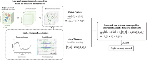
We integrate geographic knowledge into high-dimensional tensor theory and construct an urban anomaly detection and analysis framework, as shown in Figure 2.

Figure 2. Overview of urban anomaly detection and analysis framework.

Our framework comprises three parts: traffic speed extraction, traffic anomaly detection, and urban anomaly analysis. First, we preprocess the trajectory data and extract the speed on each road at each moment. Second, we construct traffic speed data into a three-dimensional tensor and then develop the ST-LRST model to decompose the observations and obtain a daily traffic tensor and a sparse anomaly tensor. Finally, we use the anomaly tensor to extract the impact duration, scope, and intensity of anomalies, and interpret the detected events with the help of crowdsourced geographic information such as points of interest (POIs) and social media.

In what follows, we briefly introduce the traffic speed extraction method because this technology is relatively mature. We focus on the detection and analysis part of urban anomalies, which are the main innovations of this study.

4.2. Traffic speed extraction

Traffic speed and flow data are prerequisites for traffic anomaly detection. The sampling interval of floating vehicle trace data is usually in the range of 20–60 s due to the limitations of positioning and communication capabilities (Fang et al. 2022). To detect the urban road traffic status using low-frequency trace data, the process includes three steps: trajectory data filtering, map matching, and traffic speed extraction. For trajectory data filtering, we refer to the methods of Chen et al. (2014) and Tang et al. (2017) to filter data that show substantial positioning drift and serious errors in the travel speed or direction angle. We use HMM for map matching, which is currently considered the mainstream algorithm (Yu et al. 2021). Furthermore, we define the average speed as a vehicle’s speed from entering a road segment to leaving it. In addition, the traffic flow speed is defined as the mean of the average speeds of vehicles within the aggregation interval, as shown in Eq. (5).

(5) $V_{t,k}=\frac{\sum _{i=1}^{n_{t,k}}\frac{dis(P_{t,k}^{entry},P_{t,k}^{exit})}{t_{t,k}^{exit}-t_{t,k}^{entry}}}{n_{t,k}},$(5)

where V_t,k, n_t,k denote the average speed and traffic volume in time interval t of road k, respectively. The aggregation time interval is typically on the order of 5–15 minutes (Thomas, Weijermars, and Van Berkum 2009), and 10 minutes is taken in this study. $P_{t,k}^{entry}$, $P_{t,k}^{exit}$ denote the trajectory points entering and exiting road k, respectively; and $t_{t,k}^{entry}$, $t_{t,k}^{exit}$ denote the corresponding time stamps. dis (i, j) represents the distance between trajectory points i and j in the road network. Detailed descriptions can be found in Kan et al. (2019), Fang et al. (2022).

4.3. Urban anomaly detection with ST-LRST model

4.3.1. Problem definition

Due to the interconnection of road segments (Saberi et al. 2020) and the periodicity of crowd movement (Schläpfer et al. 2021), we organize the traffic data as a third-dimensional tensor $\mathcal{X}$∈R ^M×N×T (i.e. M road segments - N time intervals/day - T days) and impose a low-rank assumption on $\mathcal{X}$.

Based on the preceding analysis, the urban road traffic status can be interpreted as a combination of daily regular activity flows (represented by a low-rank tensor $\mathcal{L}$), and nonregular anomalies (captured by a sparse tensor $\mathcal{S}$). To this end, the anomaly detection problem in the coexistence of potential anomalies can be formulated using the following equation, i.e.

(6) $\begin{array}{rl}& arg\underset{\mathcal{L},\mathcal{S}}{min}rank(\mathcal{L})+\lambda {∥\mathcal{S}∥}_0\\ & s.t.\mathcal{X}=\mathcal{L}+\mathcal{S}\end{array}.$(6)

4.3.2. Low-rank sparse tensor model based on TNN

As described above, due to the non-convexity of L0-norm and the discontinuity of the rank function, equation (6)(6) $\begin{array}{rl}& arg\underset{\mathcal{L},\mathcal{S}}{min}rank(\mathcal{L})+\lambda {∥\mathcal{S}∥}_0\\ & s.t.\mathcal{X}=\mathcal{L}+\mathcal{S}\end{array}.$(6) ‘s optimization is proven to be NP-hard (Hillar and Lim 2013).

As L1-norm is a convex approximation of element-wise matrix sparsity and is more robust to noise than L2-norm, it can be used to capture sparsity better (Candès et al. 2011). For the nonconvex rank function, we propose extending the truncated nuclear norm of the matrix to a high-dimensional tensor and using it as a tighter approximation of the low-rank tensor. For subsequent elaboration, the definition of the matrix truncated nuclear norm is given below, i.e. Lemma 1.

Lemma 1

(Cao et al. 2017; Hu et al. 2012) Suppose X$\in$R^m×n is any given matrix; m, n, and r are any non-negative integers. The singular value decomposition (SVD) of matrix X is denoted as X= UΣV^T, where U = (u₁, u₂, … , u_m)$\in$R^m×m, Σ$\in$R^m×n, and V = (v₁, v₂, … , v_n)$\in$R^n×n. Let A = (u₁, u₂, … , u_r) ^T, B = (v₁, v₂, … , v_r) ^T (r ≤ min(m, n)), then

$\underset{A{A}^T=I_{r\times r},B{B}^T=I_{r\times r}}{max}Tr(AX{B}^T)=\sum _{i=1}^r{\sigma }_i(X).$

Therefore,

(7) ${∥X∥}_r=\sum _{i=r+1}^{min(m,n)}{\sigma }_i(X)={∥X∥}_{\ast }-\underset{A{A}^{\mathrm{\top }}=I_{r\times r},B{B}^{\mathrm{\top }}=I_{r\times r}}{max}Tr(AX{B}^T).$(7)

Thus, we propose the following definition of the tensor truncated nuclear norm:

(8) ${∥\mathcal{X}∥}_r=\sum _{k=1}^d{\alpha }_k{∥{\mathcal{X}}_{(k)}∥}_{r_k},$(8)

where α_ks are constants satisfying α_k ≥0 and $\sum _{k=1}^n{\alpha }_k=1,r_k=⌈\theta \cdot min\left\{n_k,\prod _{h\ne k}{n}_h\right\}⌉,\mathrm{\forall }k\in \{1,$2,…,d}.

Essentially, the truncated nuclear norm of a tensor is a combination of the truncated nuclear norms of all matrices unfolded in each mode (Liu et al. 2012; Chen, Yang, and Sun 2020). Note that when the mode number n = 2 (i.e. matrix), the truncated nuclear norm of a tensor is consistent with the matrix case. So far, Eq. (6) can be expressed as follows:

(9) $\begin{array}{rl}& \underset{\mathcal{L},\mathcal{S},\mathcal{N}}{min}{∥\mathcal{L}∥}_r+{\lambda }_1{∥\mathcal{S}∥}_1\\ s.t.& {\mathcal{P}}_{\mathrm{\Omega }}(\mathcal{L}+\mathcal{S})={\mathcal{P}}_{\mathrm{\Omega }}(\mathcal{X})\end{array}.$(9)

In this way, compared with the convex function (nuclear norm approximation), the truncated nuclear norm achieves a more accurate approximation of daily traffic patterns. However, the above model ignores the unique spatiotemporal properties of urban traffic data, hindering their application to anomaly detection in complex urban scenarios (Wang and L 2021).

4.3.3. Introduction of spatio-temporal characteristics of urban traffic anomalies

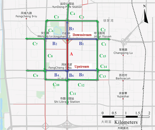
In fact, unlike other types of anomalies, traffic anomalies often have distinct spatial and temporal properties. Specifically, the abnormal traffic status of a road in the road network is neither transient nor independent. It typically continuously affects the traffic status upstream and downstream, and the impact intensity is closely related to the topology of the road network (Wang et al. 2019).

In Figure 3, for example, central road A is adjacent to roads B1–B6 in the first order and C1–C15 roads in the second order. Owing to the spatial transferability of traffic flow, the traffic flow patterns of road A are similar to those of B1–B6 and C1–C15; this similarity decreases with the increase of the topological order. In other words, when a traffic accident occurs on road segment A, it directly affects the traffic status of B1–B6 road segments, which further affects C1–C15; and such urban anomalies tend to be temporally continuous.

Figure 3. Urban adjacent road topology. Central road a is adjacent to roads B1–B6 in the first order and roads C1–C15 roads in the second order.

To this end, we attempt to incorporate GIScience methods into LRST to improve the detection accuracy of anomalous traffic status. This approach is also known as manifold learning (Roweis and Saul 2000; Tenenbaum, Silva, and Langford 2000), and the main idea is that if two objects are close in the intrinsic geometric structure of the data manifold, then they should be close to each other after dimensionality reduction (Li et al. 2016; Sofuoglu and Aviyente 2022).

We preserve the relationships between the unfolding matrices of tensor data $\mathcal{X}$since each mode corresponds to a different attribute. By introducing temporal consistency and spatial topological correlation matrices in different modes, the neighboring moments and roads behave similarly in the projected low-dimensional space. In the following, we present the process of constructing the spatiotemporal correlation matrices.

• Temporal constraint matrix. Urban anomalies tend to be temporally continuous, i.e. smooth in the second mode. Consequently, when differentiating moment t from its neighboring moments, the values of the matrix mostly converge to zero with significant sparsity. Thus, we utilize a Toeplitz matrix Δ to capture this temporal continuity, as Eq. (10),

(10) $\mathrm{\Delta }=\left(\begin{array}{ccccc}1& -1& 0& 0& \cdots \\ 0& 1& -1& 0& \ddots \\ 0& 0& 1& -1& \ddots \\ ⋮& ⋮& \ddots & \ddots & \ddots \end{array}\right).$(10)

As such, Eq. (9) can be further expressed using Eq. (11):

(11) $\begin{array}{rl}& \underset{\mathcal{L},\mathcal{S},\mathcal{N}}{min}{∥\mathcal{L}∥}_r+{\lambda }_1{∥\mathcal{S}∥}_1+{\lambda }_2{∥{\mathcal{S}}_{\times 2}\mathrm{\Delta }∥}_1\\ s.t.& {\mathcal{P}}_{\mathrm{\Omega }}(\mathcal{L}+\mathcal{S})={\mathcal{P}}_{\mathrm{\Omega }}(\mathcal{X})\end{array},$(11)

where λ₁, λ₂ are nonnegative weights balancing the corresponding terms.

• Spatial constraint matrix. Theoretically, if two data points x_i and x_j are close in the intrinsic manifold, their corresponding representations z_i and z_j are also close or similar (Wang et al. 2015, 2019). In graph theory, many scholars have proposed a Laplacian regularization-based unsupervised learning method, which imposes spatially smooth constraints on connected vertices in a predefined graph (Lu, Wang, and Yuan 2013; Zhang et al. 2020). Inspired by these studies, we incorporate a Laplace regularizer into the first mode (i.e. spatial mode) unfolding matrix of the anomaly tensor to simulate the dynamic process of traffic flow diffusion, as shown in Eq. (12),

(12) $\begin{array}{rl}& \frac{1}{2}\sum _{i=1}^n\sum _{j=1}^n{a}_{ij}{∥{\mathbf{s}}_i-{\mathbf{s}}_j∥}_2^2=\sum _{i=1}^n\sum _{j=1}^n{\mathbf{s}}_i{a}_{ij}{\mathbf{s}}_i^T-\sum _{i=1}^n\sum _{j=1}^n{\mathbf{s}}_i{a}_{ij}{\mathbf{s}}_j^T\\ & =\sum _{i=1}^n{\mathbf{s}}_i{d}_{ii}{\mathbf{s}}_i^T-\sum _{i=1}^n\sum _{j=1}^n{\mathbf{s}}_i{a}_{ij}{\mathbf{s}}_j^T\\ & =Tr({\mathit{S}}^T(\mathit{D}-\mathit{A})\mathit{S})=Tr({\mathit{S}}^T{\mathit{L}}_A\mathit{S})\end{array},$(12)

where S denotes the matrix of anomaly tensor $\mathcal{S}$ unfolded in the first mode, and s_i denotes the i-th row of this matrix. ||·||₂ and Tr (·) denote the L2-norm and trace norm, respectively. L_A is a Laplacian matrix defined as:

${\text{L}}_{\text{A}}(i,j)=\{\begin{array}{cc}-a_{ij}& i\ne j\\ {\displaystyle \sum _{c=1}^n{a}_{ij}}& i=j\end{array}$

where $a_{ij}=\{\begin{array}{cc}1& iandjareneighboring,\\ 0& otherwise.\end{array}$.

4.3.4. Spatio-temporal constrained low-rank sparse tensor method

As mentioned above, we extend the truncated nuclear norm to a high-dimensional tensor to better approximate regular urban traffic flow and improve the extraction accuracy of the sparse anomaly tensor. On the other hand, for urban anomalies, a smoothing matrix is introduced in the time dimension to reflect the continuity of anomalous states, and a Laplacian regularizer is incorporated to capture the spatial transitivity of traffic flows.

To this end, the traffic anomaly tensor extracted by the algorithm not only maintains sparse characteristics but also conforms to the clustering properties of temporal continuity and spatial adjacency. This avoids the tedious spatio-temporal clustering operation required in traditional methods (Cheng et al. 2021; Zhang et al. 2019) for the detected discrete and discontinuous anomalies. In this section, we describe the low-rank sparse tensor decomposition model under the spatiotemporal constraints proposed in this study. The specific ST-LRST procedure is illustrated in Figure 4.

Figure 4. Specific ST-LRST procedure.

By now, the anomaly detection problem considering the spatiotemporal characteristics of traffic anomalies can be formulated using the following equation:

(13) $\begin{array}{rl}& \underset{\mathcal{L},\mathcal{S},\mathcal{N}}{min}{∥\mathcal{L}∥}_r+{\lambda }_1{∥\mathcal{S}∥}_1+{\lambda }_2{∥{\mathcal{S}}_{\times 2}\mathrm{\Delta }∥}_1+{\lambda }_{3}Tr({\mathcal{S}}_{(1)}^T{L}_A{\mathcal{S}}_{(1)})\\ & s.t.{\mathcal{P}}_{\mathrm{\Omega }}(\mathcal{L}+\mathcal{S})={\mathcal{P}}_{\mathrm{\Omega }}(\mathcal{X})\end{array},$(13)

where λ₁, λ₂, λ₃ are non-negative weights balancing the corresponding terms.

4.3.5. Solving ST-LRST for urban traffic anomaly detection

Based on Eq. (13), we introduce auxiliary tensor variables$\mathcal{M}$to avoid the dependence of the TNN operator on spatiotemporally constrained optimization and utilize $\mathcal{W},\mathcal{Z},\mathcal{V}$ to ensure variable optimization independence as well as the convenience of L1-norm optimization. Specifically, the optimization model is expressed as:

(14) $\begin{array}{rl}& \underset{\mathcal{L},\mathcal{S},\mathcal{N}}{min}\sum _{k=1}^3{p}_k\left({∥{\mathcal{L}}_{k(k)}∥}_{\ast }-Tr\left(A{\mathcal{L}}_{k(k)}{B}^T\right)\right)+{\lambda }_1{∥\mathcal{S}∥}_1+{\lambda }_2{∥\mathcal{Z}∥}_1\text{break}+{\lambda }_{3}Tr({\mathcal{V}}_{(1)}^T{L}_A{\mathcal{V}}_{(1)})\text{break}s.t.{\mathcal{P}}_{\mathrm{\Omega }}(\mathcal{M}+\mathcal{S})={\mathcal{P}}_{\mathrm{\Omega }}(\mathcal{X}),{\mathcal{L}}_k=\mathcal{M},\mathcal{W}=\mathcal{S},\mathcal{Z}=fol{d}_2({\mathcal{W}}_{\times 2}\mathrm{\Delta }),\mathcal{V}=\mathcal{S}\end{array},$(14)

where p_k denotes the weight of mode-k unfolding matrix.

An approach widely used to solve this optimization problem is the Alternating Direction Method of Multipliers (ADMM) framework (Boyd et al. 2011). Based on Eq. (14), we present an augmented Lagrangian function to facilitate the subsequent ADMM construction and solution. Specifically, the loss function $\mathcal{F}$ can be expressed as

(15) $\begin{array}{rl}& \mathcal{F}\left({\left[{\mathcal{L}}_k\right]}_{k=1}^3,\mathcal{S},\mathcal{W},\mathcal{Z},\mathcal{V},\mathcal{M}\right)=\sum _{k=1}^3{p}_k\left({∥{\mathcal{L}}_{k(k)}∥}_{\ast }-Tr\left(A{\mathcal{L}}_{k(k)}{B}^T\right)\right)\text{break}+{\lambda }_1{∥\mathcal{S}∥}_1+{\lambda }_2{∥\mathcal{Z}∥}_1+{\lambda }_{3}Tr({\mathcal{V}}_{(1)}^T{L}_A{\mathcal{V}}_{(1)})\\ & +\sum _{k=1}^3\left(\frac{{\rho }_k}{2}{∥{\mathcal{L}}_k-\mathcal{M}∥}_F^2+⟨{\mathcal{T}}_k,{\mathcal{L}}_k-\mathcal{M}⟩\right)+\frac{\alpha }{2}{∥\mathcal{M}+\mathcal{S}-\mathcal{X}∥}_F^2+⟨{\mathcal{Y}}_1,\mathcal{M}+\mathcal{S}-\mathcal{X}⟩+\frac{\beta }{2}{∥\mathcal{W}-\mathcal{S}∥}_F^2+⟨{\mathcal{Y}}_2,\mathcal{W}-\mathcal{S}⟩\\ & +\frac{\gamma }{2}{∥\mathcal{Z}-fol{d}_2({\mathcal{W}}_{\times 2}\mathrm{\Delta })∥}_F^2+⟨{\mathcal{Y}}_3,\mathcal{Z}-fol{d}_2({\mathcal{W}}_{\times 2}\mathrm{\Delta })⟩+\frac{\phi }{2}{∥\mathcal{V}-\mathcal{S}∥}_F^2+⟨{\mathcal{Y}}_4,\mathcal{V}-\mathcal{S}⟩\end{array}$(15)

where $⟨X,Y⟩=tr(X^{T}Y)$. ${\mathcal{T}}_k,{\mathcal{Y}}_k$ are dual variables, ${\rho }_k(k=1,2,3),\alpha ,\beta ,\gamma ,\phi >0$ are called the penalty parameters.

To this end, we can transform the large-scale anomaly detection problem in Eq. (15) into a series of subproblems, which can be solved respectively and iteratively.

(16) $\begin{array}{rl}& {\mathcal{L}}_k^{l+1}:=arg\underset{\mathcal{L}}{min}\mathcal{F}\left({\left[{\mathcal{L}}_k^{l+1}\right]}_{k=1}^3,{\mathcal{S}}^l,{\mathcal{W}}^l,{\mathcal{Z}}^l,{\mathcal{V}}^l,{\mathcal{M}}^l\right),\\ & {\mathcal{S}}^{l+1}:=arg\underset{\mathcal{S}}{min}\mathcal{F}\left({\left[{\mathcal{L}}_k^{l+1}\right]}_{k=1}^3,{\mathcal{S}}^{l+1},{\mathcal{W}}^l,{\mathcal{Z}}^l,{\mathcal{V}}^l,{\mathcal{M}}^l\right),\\ & {\mathcal{W}}^{l+1}:=arg\underset{\mathcal{W}}{min}\mathcal{F}\left({\left[{\mathcal{L}}_k^{l+1}\right]}_{k=1}^3,{\mathcal{S}}^{l+1},{\mathcal{W}}^{l+1},{\mathcal{Z}}^l,{\mathcal{V}}^l,{\mathcal{M}}^l\right),\\ & {\mathcal{Z}}^{l+1}:=arg\underset{\mathcal{Z}}{min}\mathcal{F}\left({\left[{\mathcal{L}}_k^{l+1}\right]}_{k=1}^3,{\mathcal{S}}^{l+1},{\mathcal{W}}^{l+1},{\mathcal{Z}}^{l+1},{\mathcal{V}}^l,{\mathcal{M}}^l\right),\\ & {\mathcal{V}}^{l+1}:=arg\underset{\mathcal{V}}{min}\mathcal{F}\left({\left[{\mathcal{L}}_k^{l+1}\right]}_{k=1}^3,{\mathcal{S}}^{l+1},{\mathcal{W}}^{l+1},{\mathcal{Z}}^{l+1},{\mathcal{V}}^{l+1},{\mathcal{M}}^l\right),\\ & {\mathcal{M}}^{l+1}:=arg\underset{\mathcal{M}}{min}\mathcal{F}\left({\left[{\mathcal{L}}_k^{l+1}\right]}_{k=1}^3,{\mathcal{S}}^{l+1},{\mathcal{W}}^{l+1},{\mathcal{Z}}^{l+1},{\mathcal{V}}^{l+1},{\mathcal{M}}^{l+1}\right),\end{array}$(16)

where each variable is sequentially updated from top to bottom. When the lth and l +1th updates satisfy ${∥({\mathcal{M}}^{l+1}+{\mathcal{S}}^{l+1})-({\mathcal{M}}^l+{\mathcal{S}}^l)∥}_F/{∥{\mathcal{P}}_{\mathrm{\Omega }}(\mathcal{X})∥}_F^2<\epsilon$, the algorithm has converged and the traffic anomaly tensor $\mathcal{S}$ can be output as the final result. The specific steps for urban anomaly detection are presented in Algorithm 1. For brevity, we provide the detailed formula derivation in Appendix A.

Table

Algorithm 1 Solving ST-LRST for Urban Anomaly Detection

Input: Traffic speed tensor $\mathcal{X}\in {\mathbb{R}}^{M\times N\times T}$; decomposed matrices A, B; penalty parameters ρk, α, β, γ, φ; weight parameters pk, λk (k = 1,2,3); anomaly spatiotemporal correlation matrices Δ, LA. Initialize: ${\mathcal{P}}_{\mathrm{\Omega }}({\mathcal{L}}_k^0)={\mathcal{P}}_{\mathrm{\Omega }}({\mathcal{M}}^0)={\mathcal{P}}_{\mathrm{\Omega }}(\mathcal{X})$, ${\mathcal{S}}^0={\mathcal{W}}^0={\mathcal{Z}}^0={\mathcal{V}}^0={\mathcal{T}}_k^0={\mathcal{Y}}_d^0=0\in {\mathbb{R}}^{M\times N\times T}$, (k = 1,2,3; d = 1,2,3,4); δ, ${\rho }_k^{max}$, α^max, β^max, γ^max, φ^max, ɛ, MaxIter. Iter = 0; While Iter ≤ MaxIter and not converged do Update penalty parameters using Eq. (A.18) in Appendix A; For k = 1 to 3 do Update tensors $\mathcal{L}$k via Eq. (A.5); End For Update sparse tensor $\mathcal{S}$ via Eq. (A.8); Update auxiliary tensor $\mathcal{W}$ via Eq. (A.10); Updating temporal feature tensor $\mathcal{Z}$ via Eq. (A.12); Updating spatial feature tensor $\mathcal{V}$ via Eq. (A.14); Update auxiliary tensor $\mathcal{M}$ via Eq. (A.16); Update dual variables via Eq. (A.17); Iter = Iter + 1; End While Output: Urban traffic anomaly tensor $\mathcal{S}$.

4.4. Urban traffic anomaly analysis

The understanding and characterization of traffic tensors have a wide range of applications in smart cities. In particular, the accurate perception and analysis of urban anomalies enable management to rationalize resource allocation, make appropriate decisions, and implement specific preventive measures for emerging problems (Fanaee-T and Gama 2016). However, the complexity of anomalies and the diversity of traffic state changes are critical challenges. Most researchers (Fanaee-T and Gama 2016; Xu et al. 2019) singularly classify events according to the duration or impact intensity of anomalies; however, a complete analysis framework has not yet been developed.

In general, the changes in urban traffic status can be classified into two categories: changes in road traffic flow and changes in road network topology. Furthermore, the former can be divided into citywide and partial road traffic flow changes, as listed in Table 1. In particular, we summarize the characteristics of traffic flow changes under major urban events and some prior knowledge that can be used for anomaly analysis. Note that, although both concerts and serious traffic accidents cause traffic congestion on some roads, the former tend to occur around the venue, are announced in advance, and have clear inflow and outflow processes, whereas the latter are unpredictable and mostly occur in random locations.

Table 1. Analysis of abnormal traffic status on urban roads.

Traffic Status		Event Type	Characteristics of changes	Duration	Scope of Impact	Prior knowledge
Traffic flow changes	Citywide road network	Citywide large-impact events (e.g. Olympic Games, large festivals, etc.)	Traffic increases on the whole road network	Day	Citywide	Date, POIs
		Extreme weather (typhoons, snowstorms, etc.)	Traffic reduction for the whole road network	Day	Citywide	Weather forecast
	Some road segments	Serious traffic accidents	Congestion in some areas and during some hours	Hour	Road segments	/
		Sports games and concerts	Congestion in some areas and during some hours	Hour	Road segments	Social Media, POIs
Topology changes		Road openings and closures (e.g. marathon)	Traffic status on some roads changes to 0	Hour	Road segments	Government announcement

5. Experiments

In this section, we choose an urban trajectory dataset to evaluate the validity of the proposed urban traffic anomaly and analysis framework, especially the effectiveness of ST-LRST model. Evaluating the accuracy of algorithms using real urban events is difficult because obtaining urban traffic datasets with complete ground-truth information is challenging (Sofuoglu and Aviyente 2022). Therefore, we evaluate the validity of the anomaly detection model ST-LRST using simulation experiments for model comparisons. Then, we explain the factors that induce traffic anomalies by detecting anomalies with real urban traffic data to illustrate the validity of the proposed framework.

5.1. Dataset

XA-data: The urban area of Xi’an, China, is selected as the study area. We select two months of the trajectories of moving vehicles in Xi’an as the experimental data, as shown in Figure 5. By preprocessing the trajectory data and extracting the traffic status, we obtained traffic speed data for 500 roads in the urban area of Xi’an, as shown in Table 2.

Figure 5. The urban road network in Xi’an, China. Brown lines indicate the major road segments in the study area.

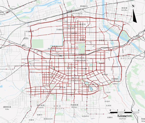
Table 2. Datasets used in this study.

Date	Duration	Resolution	Size (Matrix)	Size (Tensor)	Remarks
Apr. 2018	30 days	10min	500 × 4320	500 × 144 × 30	Simulation study, traffic flow change detection
Oct. 2018	31 days	10min	500 × 4464	500 × 144 × 31	Topology change detection

5.2. Simulation study

5.2.1. Synthetic data generation

Evaluating real-world urban events is challenging because of the lack of complete ground-truth values. To quantitatively assess the proposed method, we generate synthetic data and insert different types of anomalies. Specifically, we follow the idea described by Sofuoglu and Aviyente (2022) and utilize the constructed three-dimensional tensor to obtain the average value of road speed in Xi’an along the third mode, i.e. to obtain the average speed of each road at each moment. Then, we repeat the obtained two-dimensional matrix such that for each road segment, the daily average data are repeated 30 times to obtain the simulated data for the normal traffic status.

To quantitatively evaluate the validity and robustness of ST-LRST, we design three different scales of anomalies and insert them into normal traffic data to simulate small-, medium-, and large- scale anomalies, as shown in Table 3. In particular, the locations of the anomalies are randomly generated, and the spatially affected areas are based on the neighborhoods of the actual road network (i.e. first order, second order, etc.) to simulate the traffic state progression when real events occur. In terms of occurrence frequency, we think that small-scale events are more likely to occur than large-scale events.

Table 3. Anomalies simulated at different scales.

Type	Impact scope (Spatial)	Impact scope (Temporal)	Impact intensity	Frequency
Anomaly #1	1st order	1 h	65%	3 times a day
Anomaly #2	2nd order	3 h	55%	once a day
Anomaly #3	3rd order	12 h	40%	once every 10 days

Indeed, most current simulation experiments for traffic anomaly detection are performed by adding random numbers (Fanaee-T and Gama 2016) or multiplying by the same constant (Cheng et al. 2021; Sofuoglu and Aviyente 2022). However, since roads at different levels or in different areas have different free-flow velocities, the above simulations may deviate from real situations. Therefore, we use the ratio r of the real roadway traffic speed and free-flow ideal traffic speed to evaluate the impact degree of anomalies (Kan et al. 2019; Transport 2016), which is defined as:

(17) $r=\frac{T_{free}}{T_a}=\frac{V_a}{V_{free}},$(17)

where T_free is the free-flow travel time; T_a is the actual travel time; V_free is the free-flow speed; V_a is the actual travel speed. According to the evaluation criteria of the study area (Transport 2016), traffic status can be quantified into five categories corresponding to the five traffic conditions of r, as shown in Table 4.

Table 4. Road segment traffic operation status classification.

Traffic condition	Smooth	Basically smooth	Mild congestion	Moderate congestion	Serious congestion
r	r > 70%	50% < r ≤ 70%	40% < r ≤ 50%	30% < r ≤ 40%	r ≤ 30%

Therefore, under the assumption of impact intensity, we choose three simulation cases: basically smooth, mild congestion, and moderate congestion. The median of each scenario is used to obtain 60%, 45%, and 35% of the free flow, i.e. the impact degree on traffic status is 40%, 55%, and 65%, respectively (as shown in Table 3). To this end, we simulate 123 anomalies, including 90 small-scale, 30 medium-level, and 3 large-scale events.

5.2.2. Model evaluation criteria

The evaluation of anomaly detection results is an important step in quantitatively assessing an anomaly detection model. In this study, we provide a comprehensive assessment of the detection results from three aspects:

• Quantity: Whether an anomaly at a location can be detected;

• Scope: Whether the spatial and temporal impact scope of the anomaly is correct;

• Intensity: Whether the impact intensity analysis is accurate.

Specifically, to determine whether an anomaly is detected, we mark the detection as a hit (1) if spatial or temporal overlap occurs between the real and detected anomalies; otherwise, we mark it as a miss (0).

The accuracy of the impact scope is evaluated using three indicators: precision, recall, and F1-score. For each anomaly, we compare the number of spatiotemporal units occupied by the detected anomalies with the true annotation to calculate the precision and recall:

$precision=\frac{\left|\{Rea{l}_{\hspace{0.17em}}worl{d}_{\hspace{0.17em}}anomalou{s}_{\hspace{0.17em}}units\}\cap \{Detecte{d}_{\hspace{0.17em}}anomalou{s}_{\hspace{0.17em}}units\}\right|}{\left|\{Detecte{d}_{\hspace{0.17em}}anomalou{s}_{\hspace{0.17em}}units\}\right|},$

$recall=\frac{\left|\{Rea{l}_{\hspace{0.17em}}worl{d}_{\hspace{0.17em}}anomalou{s}_{\hspace{0.17em}}units\}\cap \{Detecte{d}_{\hspace{0.17em}}anomalou{s}_{\hspace{0.17em}}units\}\right|}{\left|\{Rea{l}_{\hspace{0.17em}}worl{d}_{\hspace{0.17em}}anomalou{s}_{\hspace{0.17em}}units\}\right|}.$

For instance, in the XA-data, the time unit is 10 minutes and the spatial unit is a single road segment. Meanwhile, we compute the F1-Score as:

$F1-Score=\frac{2\cdot precision\cdot recall}{precision+recall},$

to evaluate the performance of different models and to help select model parameters.

For the impact intensity analysis, we evaluate it from both qualitative and quantitative aspects. Qualitatively, we utilize the traffic status classification method presented in Table 4. For each anomaly, if the detected impact intensity falls within the true labeled interval, an accurate estimate is considered to be obtained; otherwise, we calculate its deviation value from the true impact intensity. For example, for an anomaly with a true labeled intensity of 55% as mild congestion, if the detected impact intensity falls within the range of mild congestion (i.e. impact intensity of 50%-60%), we consider an accurate detection is obtained; otherwise, we calculate its percentage deviation from 55%.

To more clearly visualize the accuracy of the different models in detecting impact intensity, we introduce two indicators, RMSE and MAPE, to quantitatively evaluate the difference between the detected and true anomaly intensity.

(18) $RMSE=\sqrt{\frac{\sum _{i=1}^N{(y_i-{\hat{y}}_i)}^2}{N}}MAPE=\frac{1}{N}\sum _{i=1}^N\left|\frac{y_i-{\hat{y}}_i}{y_i}\right|\times 100\mathrm{\%},$(18)

where y_i denotes the true speed of i-th anomaly event, denotes the speed estimated using the detection model, and N is the total number of anomalies.

5.2.3. Baseline methods

We select classic and recently proposed anomaly detection methods as references, which can be categorized into three groups: 1) traditional anomaly detection methods, such as isolation forest, 2) matrix anomaly detection methods, and 3) tensor anomaly detection methods, including those based on tensor decomposition and nuclear norm relaxation. Table 5 presents detailed descriptions of different baseline models. For brevity, the parameter settings of different models are presented in Appendix B and Appendix C.

Table 5. Description of different baseline models.

Data Structure		Method	Description
Vector		Isolation Forest (Liu, Ting, and Zhou 2012)	A fast outlier detection method based on Ensemble. A binomial search tree structure called isolation tree is used to perform anomaly detection for the traffic status of each road segment.
Matrix (Road segments, time intervals × days)		LRSD (TNN) (Xue et al. 2019)	A low-rank and sparse matrix decomposition method with the introduction of the truncated nuclear norm and sparse regularization for constraints.
		Improved RPCA (Wang et al. 2018)	An improved robust principal component analysis model that considers the temporal dependence of urban anomalies.
Tensor (Road segments, time-intervals, days)	Based on tensor decomposition	BATF (Chen et al. 2019)	A fully Bayesian model built on a special tensor factorization formulation that learns variables via variational Bayes.
	Based on nuclear norm relaxation	LATC (Chen et al. 2022)	A low-rank autoregressive tensor model that introduces truncated nuclear norm and temporal variation to effectively characterize both global patterns and local consistency in spatiotemporal traffic data.
		TRPCA (NN) (Hu and Work 2021)	Also named LRST, a tensor robust principal component analysis method that uses nuclear norm as a convex substitution of the rank function to extract low-rank tensors.
		TRPCA (t-SVT) (Lu et al. 2020)	A tensor robust principal component analysis method with a new tensor nuclear norm that uses tensor Singular Value Threshold (t-SVT) as the proximity operator associated with the tensor nuclear norm.

5.2.4. Anomaly detection results

To illustrate the effectiveness of the proposed ST-LRST, we use the generated simulation data to compare the anomaly detection accuracies of different algorithms.

a) Single-type anomaly detection

For single-type anomaly detection, we take the results of scope detection evaluation as an example, and present the performance differences of each algorithm for different types of anomalies in Table 6.

Table 6. Performance comparison for single-type anomaly detection. Bold values indicate the best performance among the considered models.

Scenario	Criterion	Isolation Forest	LRSD	Improved PRCA	BATF	LATC	TRPCA (NN)	TRPCA (t-SVT)	ST-LRST (Ours)
Anomaly #1	Precision	81.56%	87.18%	99.66%	81.55%	87.03%	100.00%	98.18%	100.00%
	Recall	60.03%	100.00%	96.85%	100.00%	100.00%	99.75%	100.00%	99.88%
	F1-Score	69.16%	93.15%	98.23%	89.84%	93.07%	99.88%	99.08%	99.94%
Anomaly #2	Precision	100.00%	75.77%	68.43%	67.63%	71.52%	83.76%	87.49%	97.46%
	Recall	40.65%	72.55%	100.00%	98.02%	100.00%	100.00%	100.00%	100.00%
	F1-Score	57.81%	74.13%	81.26%	80.03%	83.40%	91.16%	93.33%	98.71%
Anomaly #3	Precision	98.93%	61.61%	59.90%	28.19%	64.58%	78.21%	82.25%	96.76%
	Recall	20.56%	18.03%	100.00%	29.05%	75.60%	99.99%	100.00%	99.96%
	F1-Score	34.04%	27.90%	74.92%	28.61%	69.66%	87.77%	90.26%	98.33%

Overall, the proposed ST-LRST model achieves the best detection results under different indicators. Specifically, for Anomaly #1, most algorithms achieve the desired detection accuracy, which implies that the detection performance of the baseline models is relatively accurate for small-scale, high-intensity urban anomalies.

However, for anomalies with weak impact intensity, the performance of models based on low-rank tensors, i.e. TRPCA (NN), TRPCA (t-SVT), and ST-LRST, is substantially better than that of vector- or matrix-based methods. This is attributed to their consideration of the periodicity and their mining of low-rank patterns in traffic data. For Anomaly #3, the detection accuracies of Isolation Forest, LRSD, and BATF are relatively low. In contrast, the proposed enables high accuracy and robust anomaly detection effects in different scenarios.

b) Mixed-type anomaly detection

We mix different types of anomalies according to the frequency of urban anomalies described in Table 3, and evaluate the anomaly detection performance of each model in terms of quantity, impact scope, and impact intensity. In terms of the detection quantity, the 123 injected anomalies are detected in all models. For brevity, Table 7 compares the scope and intensity of the impacts.

Table 7. Performance comparison for mixed-type anomaly detection. Bold values indicate the best performance among different models.

Model	Scope detection			Intensity analysis
	Precision	Recall	F1-Score	Accuracy	RMSE (km/h)	MAPE
Isolation Forest	67.00%	63.12%	65.00%	14.63%	8.31	34.76%
LRSD	91.36%	64.48%	75.60%	86.18%	3.16	7.26%
Improved PRCA	84.22%	99.31%	91.14%	93.50%	1.00	5.22%
BATF	69.23%	87.82%	77.42%	80.49%	3.14	9.85%
LATC	84.84%	92.41%	88.47%	84.55%	1.56	8.85%
TRPCA (NN)	89.68%	88.06%	88.86%	92.68%	1.17	4.16%
TRPCA (t-SVT)	93.44%	92.33%	92.88%	91.06%	1.37	4.06%
LRST-TNN (ours)	86.04%	99.50%	92.28%	95.12%	0.93	4.65%
ST-LRST (ours)	97.29%	99.74%	98.50%	95.93%	0.59	3.09%

Overall, ST-LRST outperforms the state-of-the-art methods in terms of both impact scope and intensity analysis. Generally, the detection accuracies of the vector- and matrix-based algorithms are inferior to those of the tensor-based detection methods. We note that the consideration of anomalous temporal features endows Improved RPCA with higher detection accuracy on the whole. Unfortunately, BATF fails to obtain the desired detection accuracy, which indicates that the method of setting bias vectors in augmented tensor factorization may not be suitable for anomaly detection.

Among the models based on tensor nuclear norm relaxation, TRPCA and its variations tend to obtain better results than LATC, benefiting from their separate modeling of anomalous features. Specifically, both tensor-SVT and nonconvex function TNN can achieve a more accurate extraction of the normal tensor, thus improving the urban anomaly detection performance to some extent. However, compared with t-SVT, LRST-TNN is more accurate in analyzing the intensity of urban anomalies. Meanwhile, the Fourier transform performed by each iteration of TRPCA (t-SVT) is extremely time-consuming, which limits its application for large-scale urban anomaly detection.

In particular, the precision of the LRST-TNN model without anomalous spatiotemporal constraints is low because the model detects numerous meaningless scattered anomalies that are rarely observed in reality. We will discuss this issue in detail in the next subsection. Actually, in the ST-LRST model, the occurrence of anomalies tends to be temporally continuous and has spatially topological correlation properties. This ensures that most of the detected anomalies exhibit a clustered distribution, thus avoiding the misidentification of scattered anomalies. On the other hand, the incorporation of spatiotemporal constraints makes the detected anomalies smoother and more reliable, which inevitably has a slight impact on the detection of the impact intensity.

To summarize, compared with other models, the proposed ST-LRST achieves higher accuracy in analyzing the impact intensity caused by anomalies on the basis of ensuring accurate detection and reducing misclassification.

5.2.5. Ablation studies

In the following, we illustrate the superiority and necessity of introducing nonconvex rank approximation functions and anomalous spatiotemporal constraints.

a) Introduction of nonconvex functions

In this study, the TNN is used as a tighter approximation of rank functions, which enables a more accurate extraction of the daily pattern tensor $\mathcal{L}$ and thus improves the detection of the anomaly tensor $\mathcal{S}$. To demonstrate the effect of individually introducing the nonconvex function, we randomly select two roads (Roads 1 and 125) in Xi’an. Then, we visualize and analyze the daily traffic patterns extracted from the simulated data using TRPCA (based on the nuclear norm) and LRST-TNN (based on the truncated nuclear norm). The results are shown in Figure 6.

Figure 6. Daily pattern extraction results before and after the introduction of nonconvex functions. (a) road 1; (b) road 125. Blue shaded areas indicate injected anomalies.

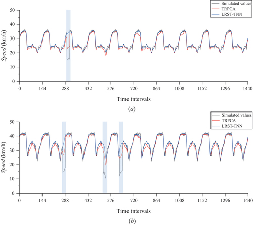
The LRST-TNN model better fits the simulation data than TRPCA with a convex substitution, i.e. LRST-TNN captures daily traffic conditions more accurately. Furthermore, LRST-TNN is more robust to the function of normal traffic patterns in the face of injected anomalies (shaded blue in Figure 6). That is, when anomalies occur, LRST-TNN can still accurately reflect the normal traffic pattern of the roadway at that moment, which also increases the accuracy of anomaly tensor detection.

b) Incorporation of anomaly spatio-temporal constraints

Above all, Table 8 quantitatively assesses the extent to which the inclusion of temporal and spatial constraints contributes to the accuracy of urban anomaly detection, respectively.

Table 8. Impact of spatial and temporal constraints on anomaly detection accuracy. Bold values indicate the best performance among different models.

Criterion	LRST-TNN	LRST-TNN + T	LRST-TNN + S	LRST-TNN + ST
Precision	86.04%	94.27%	89.09%	97.29%
Recall	99.50%	97.90%	99.56%	99.74%
F1-Score	92.28%	96.05%	94.04%	98.50%
Accuracy	95.12%	95.12%	94.31%	95.93%
RMSE (km/h)	0.93	0.76	1.10	0.59
MAPE	4.65%	3.54%	5.59%	3.09%

The experimental results indicate that compared with the incorporation of spatial constraints (LRST-TNN + S), LRST-TNN + T achieves significant improvement in both scope detection and intensity analysis. To some extent, the temporal continuity feature of sparse anomaly tensor is relatively more important for the anomaly detection task, which further confirms the different constraint weights described in Table A2 (Appendix C).

Further, we analyze the detected anomalies from both temporal and spatial perspectives to illustrate the superiority of introducing anomaly spatiotemporal constraints and to explain why the precision of LRST-TNN, as shown in Table 7, is relatively low.

We continue choosing Roads 1 and 125 as experimental objects. Temporally, for clarity and intuitiveness, we remove the anomalies from the anomaly tensor detected by different models, i.e. we retain the “non-anomalous” part of the anomaly tensor. Theoretically, the obtained residual tensor values should be zero. Indeed, Figure 7 shows the results after removing anomalies from the anomaly tensor detected using different models.

Figure 7. Anomaly detection results of different models. (a) road 1; (b) road 125.

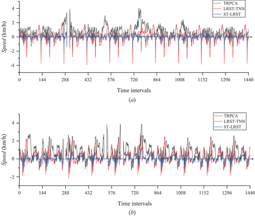
The TRPCA results have the worst sparsity, and the majority of residual values are greater than 0, since the insufficient approximation of the daily tensor $\mathcal{L}$ directly leads to deviations in the anomaly tensor $\mathcal{S}$. In addition, incorporating spatiotemporal constraints on anomalies can increase the sparsity of the detected anomaly tensor $\mathcal{S}$, i.e. the residual tensor fluctuates only within a small range around zero. Such results can reduce the false positive rate of traffic anomalies, i.e. improve the precision of anomaly detection.

Besides, the introduction of spatiotemporal constraints can improve the continuity of anomalies in spatial and temporal dimensions, and avoid the false detection of scattered anomalies. Time-192 and Time-769 are selected to display the anomaly detection results for the road status in Xi’an without (Figure 8(a)) and with (Figure 8(b)) anomalies.

Figure 8. Effect of the introduction of spatio-temporal constraints on anomaly detection results. (a) time-192, without anomalies; (b) time-769, with anomalies. |Vc| indicates the change in speed due to anomalies.

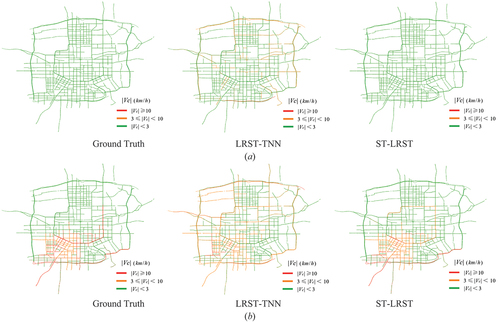
Apparently, for moments without anomalies, LRST-TNN detects many small anomalies that are sporadically distributed throughout the city. In contrast, the ST-LRST model with spatiotemporal correlations can well account for the characteristics of anomalous events and avoid the false detection of sporadic anomalies. Similarly, for situations with anomalous traffic status, ST-LRST achieves better results in terms of anomaly scope detection and impact intensity detection than LRST-TNN.

In conclusion, the proposed ST-LRST model achieves a more accurate estimation of daily traffic patterns by introducing a tighter rank approximation function, which enhances the extraction accuracy of the sparse anomaly tensor. Moreover, the incorporation of temporal continuity and spatial correlation of anomalies can reduce the misclassification rate of anomalies and achieve accurate and effective detection.

5.3. Case studies on urban anomaly analysis

To illustrate the effect of the proposed framework on real datasets, we conduct experiments in two different months (April and October) in Xi’an, corresponding to changes in traffic flow and changes in road topology, respectively. It is challenging to fully interpret the spatiotemporal anomalies of human activities due to various events and the difficulty of collecting suitable data. Instead, in each case study, we demonstrate the causes of traffic anomalies and their spatiotemporal distribution using the anomaly tensor detected by ST-LRST. By interpreting the detected abnormal traffic status, we analyze the evolution of traffic status under the influence of different events.

5.3.1. Traffic flow changes

We take changes in urban traffic during holidays as an example to analyze the evolution of traffic flow under the events. Take the Tomb Sweeping Festival in April as an example. It is a traditional Chinese festival for ancestor worship, also known as the spring outing day, a suitable day for people to travel in spring, which attracts a large number of people to gather at tourist attractions.

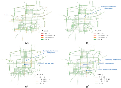
Understanding the spatial, temporal, and semantic patterns of human mobility is of great importance for urban authorities to manage these events. Using the proposed anomaly diagnosis framework, we separately detect and describe the changes in the urban road traffic during the 2018 Tomb Sweeping Festival. Meanwhile, to better explain the relationship between crowd flow and traffic anomalies, we obtained several of the most famous tourist attractions in Xi’an from social media.¹ In what follows, we analyze and illustrate the traffic anomalies detected during the Tomb Sweeping Festival (April 5).

1. 10:00 a.m.: On the first day of the holidays, many people chose to return to their hometowns for ancestral worship, and highways were free on this day. Thus, at around 10:00 a.m. (Fig. 9(a)), most of the detected traffic anomalies were distributed in the urban fringe areas or on bypass highways, which reflected the crowds gathering at highway intersections and preparing to leave the city.

2. 2:00 p.m.: As shown in Fig. 9(b), most of the crowds returning to their hometowns had already left the city, so there were no notable anomalies on the city roads. From this moment on, many people who chose to travel on holiday became active. In April, Xi’an’s weather was pleasant, and the Daming Palace National Heritage Park was full of flowers, making it a great place to trek around. We observe that around the Daming Palace National Heritage Park, traffic status began to be abnormal due to tourism.

3. 6:00 p.m.: Compared with 2:00 p.m., the anomalous traffic on city roads substantially expanded. The crowds gradually moved from the Daming Palace National Heritage Park to the Bell Tower (Fig. 9(c)). The Bell Tower is one of the most representative buildings in Xi’an and is suitable for viewing from 5:00 p.m. to 7:00 p.m. With sunset in the west, the interplay of colors can be described as splendid. Meanwhile, the crowds mainly concentrated northeast of the Xi’an Wall of the Ming Dynasty, where many restaurants and shopping malls are located.

4. 10:00 p.m.: As shown in Fig. 9(d), part of the crowd gathered inside the city wall to enjoy the gorgeous night view of the ancient city. Additionally, compared with 6:00 p.m., traffic anomalies are observed in the southeast area of the city, which corresponds to the location of Datang Everbright City. It is known as a blend of old and new Chinese culture, and is full of resplendent lights that make it suitable for visiting at night.

Figure 9. Anomaly detection map of urban roads in Xi’an on Tomb Sweeping Festival 2018. (a) 10:00 a.M. (b) 2:00 p.M. (c) 6:00 p.M. (d) 10:00 p.M. vc indicates the value of speed change due to anomalies.

5.3.2. Road topology changes

We analyze the changes in road topology due to traffic anomalies using an example involving road closures during a marathon race. On 20 October 2018, at 7:30 a.m., Xi’an hosted an international marathon race with about 30,000 participants. To guarantee the safety of the participants, the government imposed traffic controls on some roads, and the specific route map² of the marathon is shown in Figure 10(a).

Based on the proposed traffic anomaly detection and analysis framework, we detect road closures (i.e. changes in road topology) during the marathon on a one-hour timescale, and the results are shown in Figure 10(b)-(f).

Figure 10. Map of road closures detected for the 2018 Xi’an International marathon. (a) schematic diagram of the race route, with red solid lines indicating the race roads and dashed lines indicating low-grade roads. (b) 7:30 a.M. (c) 8:30 a.M. (d) 9:30 a.M. (e) 10:30 a.M. (f) 11:30 a.M.

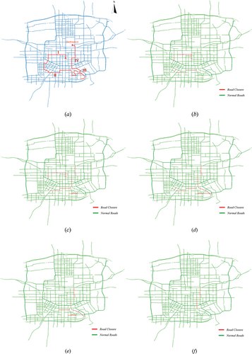
It can be seen that the roads used for the race were not all simultaneously closed. At the beginning of the race (7:30 a.m., Figure 10(b)), only the roads in the first half of the race (Sections I and II) were closed. One hour later (Figure 10(c)), the roads in Sections I, II, and IV were closed, and some roads in Section III were under control. Obviously, two hours after the start (Figure 10(d)), the roads in Sections II, III, and Ⅳ were in a state of complete closure, and at this time, Section I had resumed normal traffic. Three hours later (Figure 10(e)), the roads in Section II were lifted from closure. After four hours, only Section IV remained closed (Figure 10(f)).

Actually, the roads identified in the road detection results were not completely continuous. This is because the actual race roads contained many low-grade roads, roads along the lake, and other pedestrian-only roads (red dashed lines in Figure 10(a)), where speeds were not available in the moving vehicle GPS data. In addition, the results of road segmentation also affect the detection of road closures, as only part of the road may be closed during the actual race.

Furthermore, the closure of some roads inevitably increased traffic flow on other roads, resulting in traffic congestion or abnormal traffic. However, the question is how much did the road closures for the race affect the traffic on the surrounding roads? Actually, it is difficult to obtain directly from government documents. To address this issue, we utilize the proposed ST-LRST model to detect anomalies and evaluate the impact of the marathon on the surrounding roads. The results are shown in Figure 11.

Figure 11. Map of detected road anomalies for the 2018 Xi’an International marathon. (a) 7:30 a.M. (b) 8:30 a.M. (c) 9:30 a.M. (d) 10:30 a.M. (e) 11:30 a.M. (f) 12:30 a.M. Marathon routes are shaded in blue.

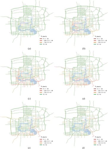
As can be seen, at the beginning of the race (Figure 11(a)), only a few roads in Section I were affected with relatively low impact intensity. As the marathon progressed, the surrounding roads exhibited different impact intensities that were consistent with the course of the marathon. Specifically, one hour after the start (8:30 a.m.), the impacted roads were mainly located around Sections I and II (Figure 11(b)). During the period from 9:30 to 10:30, roads close to Sections II and III were extensively and intensively affected (Figure 11(c)-(d)). After 11:30 a.m., the affected areas were significantly reduced (Figure 11(e)-(f)) and were mainly distributed around Section IV.

Obviously, compared with road closure detection, traffic anomaly detection can reflect the impact of running race on urban traffic status more comprehensively. Accurately and effectively detecting the urban traffic anomalies caused by races can help the government unclog and manage congested roads in advance.

6. Conclusions

Detecting and analyzing urban traffic anomalies are crucial for urban road management and smart city construction. In this study, we combined tensor theory with geographic knowledge, and proposed a comprehensive framework for traffic anomaly diagnosis based on trajectory data. This framework is divided into three parts: traffic status acquisition, traffic anomaly detection, and urban anomaly analysis.

To detect traffic anomalies, a novel ST-LRST method was constructed by integrating geographic methods into a high-dimensional tensor model. The model shows an enhanced ability to detect urban traffic anomalies in two aspects: 1) the introduction of the nonconvex alternative increased the accuracy of estimates of daily traffic patterns, thus improving the extraction accuracy of the sparse anomaly tensor; 2) the spatiotemporal correlation features of traffic anomalies were introduced into the sparse tensor to reduce the fragmentation and error rate when identifying urban traffic anomalies.

To analyze these anomalies, we studied the characteristics of anomaly duration, impact scope, and impact intensity using the anomaly tensor detected by ST-LRST. Combined with crowdsourced geographic information, we conducted comprehensive analyses of abnormal traffic status variations and identified the factors that cause urban traffic anomalies.

Thorough experiments demonstrated the superiority of the proposed framework. Incorporating GIScience methods allows the tensor model to better diagnose complex urban traffic anomalies, and introducing high-dimensional tensor theory into geospatial analysis provides a better way to reveal the intrinsic structure of complex spatiotemporal data. The results of experiments with two real events (changes in traffic flow and road network) demonstrated the application of crowdsourced geographic information for urban anomaly analysis and attribution. Overall, by integrating GIScience methods with tensor theory, we developed an anomaly diagnosis model for complex urban scenes, thereby promoting the application of GeoAI in smart cities.

Data and codes availability statement

The authors thank the DIDI Chuxing for providing the data used in this paper. Data source: DIDI Chuxing GAIA Initiative (https://sts.didiglobal.com).

Disclosure statement

No potential conflict of interest was reported by the author(s).

Additional information

Funding

This research was supported by the Fundamental Research Funds for the Central Universities, National Natural Science Foundation of China [41971405, 41671442, 42271449, 41901394], and National Key Research and Development Program of China [2023YFB3906803].

Notes

1. https://you.ctrip.com/sight/xian7.html

2. http://www.xa.gov.cn/

Appendix A.

Solving ST-LRST for urban traffic anomaly detection

For the lth iteration of the ST-LRST model, the variables optimization problem in Eq. (16)(16) $\begin{array}{rl}& {\mathcal{L}}_k^{l+1}:=arg\underset{\mathcal{L}}{min}\mathcal{F}\left({\left[{\mathcal{L}}_k^{l+1}\right]}_{k=1}^3,{\mathcal{S}}^l,{\mathcal{W}}^l,{\mathcal{Z}}^l,{\mathcal{V}}^l,{\mathcal{M}}^l\right),\\ & {\mathcal{S}}^{l+1}:=arg\underset{\mathcal{S}}{min}\mathcal{F}\left({\left[{\mathcal{L}}_k^{l+1}\right]}_{k=1}^3,{\mathcal{S}}^{l+1},{\mathcal{W}}^l,{\mathcal{Z}}^l,{\mathcal{V}}^l,{\mathcal{M}}^l\right),\\ & {\mathcal{W}}^{l+1}:=arg\underset{\mathcal{W}}{min}\mathcal{F}\left({\left[{\mathcal{L}}_k^{l+1}\right]}_{k=1}^3,{\mathcal{S}}^{l+1},{\mathcal{W}}^{l+1},{\mathcal{Z}}^l,{\mathcal{V}}^l,{\mathcal{M}}^l\right),\\ & {\mathcal{Z}}^{l+1}:=arg\underset{\mathcal{Z}}{min}\mathcal{F}\left({\left[{\mathcal{L}}_k^{l+1}\right]}_{k=1}^3,{\mathcal{S}}^{l+1},{\mathcal{W}}^{l+1},{\mathcal{Z}}^{l+1},{\mathcal{V}}^l,{\mathcal{M}}^l\right),\\ & {\mathcal{V}}^{l+1}:=arg\underset{\mathcal{V}}{min}\mathcal{F}\left({\left[{\mathcal{L}}_k^{l+1}\right]}_{k=1}^3,{\mathcal{S}}^{l+1},{\mathcal{W}}^{l+1},{\mathcal{Z}}^{l+1},{\mathcal{V}}^{l+1},{\mathcal{M}}^l\right),\\ & {\mathcal{M}}^{l+1}:=arg\underset{\mathcal{M}}{min}\mathcal{F}\left({\left[{\mathcal{L}}_k^{l+1}\right]}_{k=1}^3,{\mathcal{S}}^{l+1},{\mathcal{W}}^{l+1},{\mathcal{Z}}^{l+1},{\mathcal{V}}^{l+1},{\mathcal{M}}^{l+1}\right),\end{array}$(16) can be expressed as

a. Updating tensors $\mathcal{L}$_k (k = 1,2,3)

For each mode k, the update of traffic data tensor $\mathcal{L}$_k is denoted as

(A.1) $\begin{array}{rl}& {\mathcal{L}}_k^{l+1}:=arg\underset{\mathcal{L}}{min}{p}_k^l\left({∥{\mathcal{L}}_{k(k)}^{l+1}∥}_{\ast }-Tr\left(A{\mathcal{L}}_{k(k)}^{l+1}{B}^T\right)\right)+\frac{{\rho }_k^l}{2}{∥{\mathcal{L}}_{k(k)}^{l+1}-{\mathcal{M}}_{(k)}^l∥}_F^2+⟨{\mathcal{T}}_{k(k)}^l,{\mathcal{L}}_{k(k)}^{l+1}-{\mathcal{M}}_{(k)}^l⟩\\ & =arg\underset{\mathcal{L}}{min}\frac{p_k^l}{{\rho }_k^l}{∥{\mathcal{L}}_{k(k)}^{l+1}∥}_{\ast }+\frac{1}{2}{∥{\mathcal{L}}_{k(k)}^{l+1}-\left({\mathcal{M}}_{(k)}^l+\frac{1}{{\rho }_k^l}\left(p_k^l{A}^{T}B-{\mathcal{T}}_{k(k)}^l\right)\right)∥}_F^2\end{array}.$(A.1)

Here, we introduce Lemma 2 to solve the above optimization problem (A.1).

Lemma 2

(Cai, Candès, and Shen 2010; Cao et al. 2017) For μ > 0, and any given matrix Q∈R^m×n with rank r, the unique closed-form solution to the problem

(A.2) $L^{\ast }=\arg \underset{L}{\min }\mu {\Vert L\Vert }_{\ast }+\frac{1}{2}{\Vert L-Q\Vert }_F^2$(A.2)

takes the form

(A.3) $L^{\ast }={\mathcal{D}}_{\mu }(Q)\in {\mathbb{R}}^{m\times n},$(A.3)

where the operator ${\mathcal{D}}_{\mu }(\cdot )$ is defined by

(A.4) ${\mathcal{D}}_{\mu }(Q):=Udiag[max(\sigma -\mu ,0)]V^T,$(A.4)

U∈R^m×r, V∈R ^r×n, and σ = (σ₁, σ₂, … , σ_r)^T∈R ^r×1 are obtained by the SVD of Q, i.e., Q=Udiag(σ)V^T.

According to Lemma 2, the nuclear norm minimization problem in Eq. (A.1) has a closed-form solution by means of the $\mathcal{D}$ operator:

(A.5) ${\mathcal{L}}_k^{l+1}=fol{d}_k\left\{D_{\frac{p_k^l}{{\rho }_k^l}}\left({\mathcal{M}}_{(k)}^l+\frac{1}{{\rho }_k^l}\left(A^{T}B-{\mathcal{T}}_{k(k)}^l\right)\right)\right\}.$(A.5)

b. Updating sparse tensor $\mathcal{S}$

Optimization of tensor $\mathcal{S}$ requires consideration of the sparsity of $\mathcal{S}$and the auxiliary tensor $\mathcal{W}$$\mathcal{V}$. The minimization of $\mathcal{S}$makes the detected anomalies sparse, temporally continuous, and spatially connected, whose update equation can be expressed as:

(A.6) $\begin{array}{rl}& {\mathcal{S}}^{l+1}=arg\underset{\mathcal{S}}{min}{\lambda }_1^l{∥{\mathcal{S}}^{l+1}∥}_1+\frac{{\alpha }^l}{2}{∥{\mathcal{M}}^l+{\mathcal{S}}^{l+1}-\mathcal{X}∥}_F^2+⟨{\mathcal{Y}}_1^l,{\mathcal{M}}^l+{\mathcal{S}}^{l+1}-\mathcal{X}⟩\\ & +\frac{{\beta }^l}{2}{∥{\mathcal{W}}^l-{\mathcal{S}}^{l+1}∥}_F^2+⟨{\mathcal{Y}}_2^l,{\mathcal{W}}^l-{\mathcal{S}}^{l+1}⟩+\frac{{\phi }^l}{2}{∥{\mathcal{V}}^l-{\mathcal{S}}^{l+1}∥}_F^2+⟨{\mathcal{Y}}_4^l,{\mathcal{V}}^l-{\mathcal{S}}^{l+1}⟩\\ & =arg\underset{\mathcal{S}}{min}\frac{{\lambda }_1^l}{{\alpha }^l+{\beta }^l+{\phi }^l}{∥{\mathcal{S}}^{l+1}∥}_1+\frac{1}{2}{∥{\mathcal{S}}^{l+1}-{\mathcal{H}}^{l+1}∥}_F^2\end{array},$(A.6)

where ${\mathcal{H}}^{l+1}=\frac{{\alpha }^l(\mathcal{X}-{\mathcal{M}}^l+\frac{{\mathcal{Y}}_1^l}{{\alpha }^l})+{\beta }^l({\mathcal{W}}^l+\frac{{\mathcal{Y}}_2^l}{{\beta }^l})+{\phi }^l({\mathcal{V}}^l+\frac{{\mathcal{Y}}_4^l}{{\phi }^l})}{{\alpha }^l+{\beta }^l+{\phi }^l}$.

For the joint optimization of the L1-norm and the Frobenius norm (Peng et al. 2016), we introduce Lemma 3 to obtain a closed-form solution of Eq. (A.6) (Liu and YE 2010).

Lemma 3

(Liu and YE 2010) For a given matrix $V\in {\mathbb{R}}^{d\times n}$, the optimal solution E* to the problem:

(A.7) $\underset{E}{\min }\lambda {\Vert E\Vert }_1+\frac{1}{2}{\Vert E-V\Vert }_F^2$(A.7)

can be written as E*=S_λ [v], where v is an element of the matrix V, and S_λ [x] is a shrinkage operator defined as $S_{\lambda }[x]=sgn(x)\odot max\left\{|x|-\lambda ,0\right\}$.

When we extend the shrinkage operator to three dimensions (Wang et al. 2018), then we can update as:

(A.8) $\begin{array}{rl}& {\mathcal{S}}^{l+1}=S_{{\lambda }_1^l/({\alpha }^l+{\beta }^l+{\phi }^l)}[{\mathcal{H}}^{l+1}]\\ & =sgn({\mathcal{H}}^{l+1})\odot max\left(\left|{\mathcal{H}}^{l+1}\right|-\frac{{\lambda }_1^l}{{\alpha }^l+{\beta }^l+{\phi }^l},0\right)\end{array},$(A.8)

where ${\mathcal{H}}^{l+1}=\frac{{\alpha }^l(\mathcal{X}-{\mathcal{M}}^l+\frac{{\mathcal{Y}}_1^l}{\alpha })+{\beta }^l({\mathcal{W}}^l+\frac{{\mathcal{Y}}_2^l}{\beta })+{\phi }^l({\mathcal{V}}^l+\frac{{\mathcal{Y}}_4^l}{\phi })}{{\alpha }^l+{\beta }^l+{\phi }^l}$.

c. Updating tensor $\mathcal{W}$

The update of auxiliary tensor $\mathcal{W}$ is denoted as

(A.9) $\begin{array}{rl}& {\mathcal{W}}^{l+1}=arg\underset{\mathcal{W}}{min}\frac{{\beta }^l}{2}{∥{\mathcal{W}}^{l+1}-{\mathcal{S}}^{l+1}∥}_F^2+⟨{\mathcal{Y}}_2^l,{\mathcal{W}}^{l+1}-{\mathcal{S}}^{l+1}⟩+\frac{{\gamma }^l}{2}{∥{\mathcal{Z}}^l-fold({\mathcal{W}}_{\times 2}^{{ }^{l+1}}\mathrm{\Delta })∥}_F^2+⟨{\mathcal{Y}}_3^l,{\mathcal{Z}}^l-fold({\mathcal{W}}_{\times 2}^{{ }^{l+1}}\mathrm{\Delta })⟩\\ & =arg\underset{\mathcal{W}}{min}\frac{{\beta }^l}{2}{∥{\mathcal{W}}^{l+1}-{\mathcal{S}}^{l+1}\hspace{0.17em}+\frac{{\mathcal{Y}}_2^l}{{\beta }^l}∥}_F^2+\frac{{\gamma }^l}{2}{∥{\mathcal{Z}}^l-fold({\mathcal{W}}_{\times 2}^{{ }^{l+1}}\mathrm{\Delta })+\frac{{\mathcal{Y}}_3^l}{\gamma }∥}_F^2\end{array}.$(A.9)

Thus, the optimization update for each ${\mathcal{W}}^{l+1}$ is

(A.10) ${\mathcal{W}}^{l+1}=fol{d}_2\left({\left({\beta }^{l}I+{\gamma }^l{\mathrm{\Delta }}^T\mathrm{\Delta }\right)}^{-1}\left({\beta }^l({\mathcal{S}}_{(2)}^{l+1}-\frac{{\mathcal{Y}}_{2(2)}^l}{{\beta }^l})+{\gamma }^l{\mathrm{\Delta }}^T({\mathcal{Z}}_{(2)}^l+\frac{{\mathcal{Y}}_{3(2)}^l}{{\gamma }^l})\right)\right).$(A.10)

d. Updating tensor $\mathcal{Z}$

The update of tensor $\mathcal{Z}$ is based on the temporal continuity of anomalies. Similarly, we should consider

(A.11) $\begin{array}{rl}& {\mathcal{Z}}^{l+1}=arg\underset{\mathcal{Z}}{min}{\lambda }_2^l{∥{\mathcal{Z}}^{l+1}∥}_1+\frac{{\gamma }^l}{2}{∥{\mathcal{Z}}^{l+1}-fold({\mathcal{W}}_{\times 2}^{l+1}\mathrm{\Delta })∥}_F^2+⟨{\mathcal{Y}}_3^l,{\mathcal{Z}}^{l+1}-fold({\mathcal{W}}_{\times 2}^{l+1}\mathrm{\Delta })⟩\\ & =arg\underset{\mathcal{Z}}{min}\frac{{\lambda }_2^l}{{\gamma }^l}{∥{\mathcal{Z}}^{l+1}∥}_1+\frac{1}{2}{∥{\mathcal{Z}}^{l+1}-fold({\mathcal{W}}_{\times 2}^{l+1}\mathrm{\Delta })+\frac{{\mathcal{Y}}_3^l}{{\gamma }^l}∥}_F^2\end{array}.$(A.11)

By using the shrinkage operator introduced in Lemma 3, a closed-form solution of the optimization problem Eq. (A.11) is

(A.12) $\begin{array}{rl}& {\mathcal{Z}}^{l+1}=S_{{\lambda }_2^l/{\gamma }^l}[{\mathcal{J}}^{l+1}]\\ & =sgn({\mathcal{J}}^{l+1})\odot max\left(\left|{\mathcal{J}}^{l+1}\right|-\frac{{\lambda }_2^l}{{\gamma }^l},0\right)\end{array},$(A.12)

where ${\mathcal{J}}^{l+1}=fold({\mathcal{W}}_{\times 2}^{l+1}\mathrm{\Delta })-\frac{{\mathcal{Y}}_3^l}{{\gamma }^l}$.

e. Updating tensor $\mathcal{V}$

The update of tensor $\mathcal{V}$ considers the continuous spatial distribution of urban anomalies. Minimization of $\mathcal{V}$ enables similar traffic states between topologically connected segments, whose update equation is expressed as:

(A.13) $\begin{array}{rl}& {\mathcal{V}}^{l+1}=arg\underset{\mathcal{V}}{min}{\lambda }_3^{l}Tr({\mathcal{V}}_{(1)}^{l+1^T}{L}_A{\mathcal{V}}_{(1)}^{l+1})+\frac{{\phi }^l}{2}{∥{\mathcal{V}}^{l+1}-{\mathcal{S}}^{l+1}∥}_F^2+⟨{\mathcal{Y}}_4^l,{\mathcal{V}}^{l+1}-{\mathcal{S}}^{l+1}⟩\\ & =arg\underset{\mathcal{V}}{min}{\lambda }_3^{l}Tr({\mathcal{V}}_{(1)}^{l+1^T}{L}_A{\mathcal{V}}_{(1)}^{l+1})+\frac{{\phi }^l}{2}{∥{\mathcal{V}}^{l+1}-{\mathcal{S}}^{l+1}+\frac{{\mathcal{Y}}_4^l}{{\phi }^l}∥}_F^2\end{array}.$(A.13)

Thus, we can get its solution as follows:

(A.14) ${\mathcal{V}}^{l+1}=fol{d}_1\left({\left(2{\lambda }_3^l{L}_A+{\phi }^{l}I\right)}^{-1}\left({\phi }^l{\mathcal{S}}_{(1)}^{l+1}-{\mathcal{Y}}_{4(1)}^l\right)\right).$(A.14)

f. Updating the auxiliary tensor $\mathcal{M}$

The auxiliary tensor $\mathcal{M}$ optimization equation can be obtained from Eq. (16), which connects the original traffic data tensor $\mathcal{X}$ and the auxiliary tensor $\mathcal{L}$_k (k = 1,2,3), i.e.

(A.15) ${\mathcal{M}}^{l+1}=arg\underset{\mathcal{M}}{min}\sum _{k=1}^3\left(\frac{{\rho }_k^l}{2}{∥{\mathcal{L}}_k^l-{\mathcal{M}}^{l+1}∥}_F^2+⟨{\mathcal{T}}_k^l,{\mathcal{L}}_k^l-{\mathcal{M}}^{l+1}⟩\right)+\frac{{\alpha }^l}{2}{∥{\mathcal{M}}^{l+1}+{\mathcal{S}}^{l+1}-\mathcal{X}∥}_F^2+⟨{\mathcal{Y}}_1^l,{\mathcal{M}}^{l+1}+{\mathcal{S}}^{l+1}-\mathcal{X}⟩.$(A.15)

Then, the optimization update of tensor $\mathcal{M}$^l+1 is

(A.16) ${\mathcal{M}}^{l+1}=\frac{1}{\sum _{k=1}^3{\rho }_k^l+{\alpha }^l}\left[\sum _{k=1}^3\left({\rho }_k^l{\mathcal{L}}_k^l+{\mathcal{T}}_k^l\right)+{\alpha }^l\left(\mathcal{X}-{\mathcal{S}}^{l+1}-\frac{{\mathcal{Y}}_1^l}{{\alpha }^l}\right)\right].$(A.16)

g. Updating dual variables

Finally, we update the dual variables and parameters as follows:

(A.17) $\begin{array}{rl}& {\mathcal{T}}_k^{l+1}={\mathcal{T}}_k^l+{\rho }_k^l({\mathcal{L}}_k^{l+1}-{\mathcal{M}}^{l+1}),(k=1,2,3);\\ & {\mathcal{Y}}_1^{l+1}={\mathcal{Y}}_1^l+{\alpha }^l({\mathcal{M}}^{l+1}+{\mathcal{S}}^{l+1}-\mathcal{X});{\mathcal{Y}}_2^{l+1}={\mathcal{Y}}_2^l+{\beta }^l({\mathcal{W}}^{l+1}-{\mathcal{S}}^{l+1});\\ & {\mathcal{Y}}_3^{l+1}={\mathcal{Y}}_3^l+{\gamma }^l({\mathcal{Z}}^{l+1}-fold({\mathcal{W}}_{\times 2}^{l+1}\mathrm{\Delta }));{\mathcal{Y}}_4^{l+1}={\mathcal{Y}}_4^l+{\phi }^l({\mathcal{V}}^{l+1}-{\mathcal{S}}^{l+1}).\end{array}$(A.17)

(A.18) $\begin{array}{rl}& {\rho }_k^{l+1}=min\left(\delta {\rho }_k^l,{\rho }_k^{max}\right),(k=1,2,3);{\alpha }^{l+1}=min\left(\delta {\alpha }^l,{\alpha }^{max}\right)\\ & {\beta }^{l+1}=min\left(\delta {\beta }^l,{\beta }^{max}\right);{\gamma }^{l+1}=min\left(\delta {\gamma }^l,{\gamma }^{max}\right);{\phi }^{l+1}=min\left(\delta {\phi }^l,{\phi }^{max}\right)\end{array},$(A.18)

where δ > 1 is a constant.

So far, we have completed one step update of all variables. If the convergence condition in Algorithm 1 is met, the iteration terminates.

Appendix B.

Parameter selection for baseline models

The most important parameter in Isolation Forest is the ratio of anomalies, which we set to 0.025 based on the scale of anomalies injected in the simulation experiment. Following Xue et al. (2019), we set$\hspace{0.17em}\lambda =1/\sqrt{\mathrm{m}\mathrm{a}\mathrm{x}(I_1,I_2,I_3)}$ for LRSD and $\rho =1/(4std(vec(\mathcal{Y})))$, where $vec(\mathcal{Y})$ is the vectorization of $\mathcal{Y}$ and std (·) is the standard deviation. As for Improved RPCA, we set λ₁ = 10⁻¹, λ₂ = 10⁻³, and μ = 5 × 10⁻⁴ to maximize the detection accuracy.

For BATF, we follow the setting method in Chen et al. (2019). Specifically, we select the low-rank r and variational posterior parameters by cross-validation, and finally set r = 5, a₀ = b₀ = 10⁻². Meanwhile, the number of burn-in and Gibbs iterations are set to 1000 and 200, respectively. For LATC and TRPCA (NN), we utilize cross-validation to select the best parameters. In terms of TRPCA (t-SVT), we follow Lu et al. (2020) and set $\lambda =1/\sqrt{I_3\times \mathrm{m}\mathrm{a}\mathrm{x}(I_1,I_2)}$, μ = 10⁻³.

To ensure the reliability of the experimental results, we set the maximum number of iterations to 200 and set the convergence parameter ε to 10⁻³.

Appendix C.

Parameter selection for ST-LRST

In what follows, we discuss how the parameters of ST-LRST model are chosen. We chunk the data set in 7 days, and perform parameter selection and cross-validation on each sub-data set to ensure the parameters are selected reasonably and effectively. Instead of directly traversing all parameters simultaneously to seek the global optimal solution, we optimize in blocks according to the usage of parameters to obtain the local optimal solution for each block of variables, as shown in Table A1.

Table A1. Updated variables and related parameters.

Variables	$\mathcal{L}$k	$\mathcal{W}$	$\mathcal{Z}$	$\mathcal{V}$	$\mathcal{M}$	$\mathcal{S}$
Related parameters	pk, ρk	β, γ	λ2, γ	λ3, φ	ρk, α	λ1, α, β, φ

Specifically, we first fix other parameters and obtain the local optimal solution by traversing the parameters related to $\mathcal{L}$_k (i.e., p_k, ρ_k), and take them to the optimization of the next set of parameters, and so on until all variables are updated. Figure A1 shows the specific update results for each set of parameters, and we use F1-Score for model evaluation.

Figure A1. Model accuracy under different parameter settings, with axes to the power of 10.

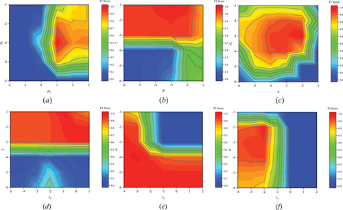
It can be seen that the model is not sensitive to the choice of other hyperparameters, except for the parameters p_k, ρ_k associated with $\mathcal{L}$_k (Figure A1(a)). Indeed, we repeated this analysis by performing it on different data and observed similar results, suggesting that the proposed method is insensitive to the selection of hyperparameters as long as they are selected within a certain range.

The final parameter settings of ST-LRST model are given in Table A2. By observing the weight parameters, we notice that the results are more inclined on the close approximation of low-rank tensor; while for sparse anomaly tensor, the model is more inclined to highlight its temporal continuity feature, which is in line with our expectation.

Table A2. Parameter settings of ST-LRST model.

Parameters	weight parameters				penalty parameters
	pk	λ1	λ2	λ3	ρk	α	β	γ	φ
Value	10^1	10^−2	10^−1	10^−3	10^−3	10^−3	10^−3	10^−1	10^−5

References

- Boyd, S., et al. 2011. “Distributed Optimization and Statistical Learning via the Alternating Direction Method of Multipliers.” Foundations & Trends® in Machine Learning 3 (1): 1–29. https://doi.org/10.1561/2200000016.
- Breunig, M. M., Kriegel H. P., Ng R. T., and J. Sander . 2000. LOF: Identifying Density-Based Local Outliers. ed. Proceedings of the 2000 ACM SIGMOD international conference on Management of data, 93–104.
- Cai, J.-F., E. J. Candès, and Z. Shen. 2010. “A Singular Value Thresholding Algorithm for Matrix Completion.” SIAM Journal on Optimization 20 (4): 1956–1982. https://doi.org/10.1137/080738970.
- Candès, E. J., X. Li, Y. Ma, and J. Wright. 2011. “Robust Principal Component Analysis?” Journal of the ACM (JACM) 58 (3): 1–37. https://doi.org/10.1145/1970392.1970395.
- Cao, F., J. Chen, H. Ye, J. Zhao, and Z. Zhou. 2017. “Recovering Low-Rank and Sparse Matrix Based on the Truncated Nuclear Norm.” Neural Networks 85:10–20. https://doi.org/10.1016/j.neunet.2016.09.005.
- Carroll, J. D., and J.-J. Chang. 1970. “Analysis of Individual Differences in Multidimensional Scaling via an N-Way Generalization of “Eckart-Young” Decomposition.” Psychometrika 35 (3): 283–319. https://doi.org/10.1007/BF02310791.
- Cheng, X. M., Z. Wang, X. Yang, L. Xu, and Y. Liu. 2021. “Multi-Scale Detection and Interpretation of Spatio-Temporal Anomalies of Human Activities Represented by Time-Series.” Computers Environment and Urban Systems 88:101627. https://doi.org/10.1016/j.compenvurbsys.2021.101627.
- Chen, X., Z. He, Y. Chen, Y. Lu, and J. Wang. 2019. “Missing Traffic Data Imputation and Pattern Discovery with a Bayesian Augmented Tensor Factorization Model.” Transportation Research Part C: Emerging Technologies 104:66–77. https://doi.org/10.1016/j.trc.2019.03.003.
- Chen, L., J. Jakubowicz, D. Yang, D. Zhang, and G. Pan. 2017. “Fine-Grained Urban Event Detection and Characterization Based on Tensor Cofactorization.” IEEE Transactions on Human-Machine Systems 47 (3): 380–391. https://doi.org/10.1109/THMS.2016.2596103.
- Chen, X., M. Lei, N. Saunier, and L. Sun. 2022. “Low-Rank Autoregressive Tensor Completion for Spatiotemporal Traffic Data Imputation.” IEEE Transactions on Intelligent Transportation Systems 23 (8): 12301–12310. https://doi.org/10.1109/TITS.2021.3113608.
- Chen, X., J. Yang, and S. Sun. 2020. “A nonconvex low-rank tensor completion model for spatiotemporal traffic data imputation.” Transportation Research Part C: Emerging Technologies 117:102673. https://doi.org/10.1016/j.trc.2020.102673.
- Chen, B. Y., H. Yuan, Q. Li, W. H. K. Lam, S.-L. Shaw, and K. Yan. 2014. “Map-Matching Algorithm for Large-Scale Low-Frequency Floating Car Data.” International Journal of Geographical Information Science 28 (1): 22–38. https://doi.org/10.1080/13658816.2013.816427.
- Fanaee-T, H., and J. Gama. 2016. “Event Detection from Traffic Tensors: A Hybrid Model.” Neurocomputing 203:22–33. https://doi.org/10.1016/j.neucom.2016.04.006.
- Fang, M., L. Tang, X. Yang, Y. Chen, C. Li, and Q. Li. 2022. “FTPG: A Fine-Grained Traffic Prediction Method with Graph Attention Network Using Big Trace Data.” IEEE Transactions on Intelligent Transportation Systems 23 (6): 5163–5175. https://doi.org/10.1109/TITS.2021.3049264.
- Harshman, R. A. 1970. “Foundations of the PARAFAC Procedure: Models and Conditions for an“explanatory” Multimodal Factor Analysis.”
- Hillar, C. J., and L.-H. Lim. 2013. “Most tensor problems are NP-hard.” Journal of the ACM (JACM) 60 (6): 1–39. https://doi.org/10.1145/2512329.
- Hu, Y., and D. B. Work. 2021. “Robust Tensor Recovery with Fiber Outliers for Traffic Events.” ACM Transactions on Knowledge Discovery from Data 15 (1): 1–27. https://doi.org/10.1145/3417337.
- Hu, Y., D. Zhang, J. Ye, X. Li, and X. He. 2012. “Fast and accurate matrix completion via truncated nuclear norm regularization.” IEEE Transactions on Pattern Analysis and Machine Intelligence 35 (9): 2117–2130. https://doi.org/10.1109/TPAMI.2012.271.
- Jiang, Z., Y. Liu, X. Fan, C. Wang, J. Li, and L. Chen. 2020. “Understanding Urban Structures and Crowd Dynamics Leveraging Large-Scale Vehicle Mobility Data.” Frontiers of Computer Science 14 (5): 1–12. https://doi.org/10.1007/s11704-019-9034-z.
- Kan, Z., Tang, L., Kwan, M-P., Ren, C., Liu, D., and Li, Q. 2019. “Traffic Congestion Analysis at the Turn Level Using Taxis’ GPS Trajectory Data.” Computers, Environment and Urban Systems 74:229–243. https://doi.org/10.1016/j.compenvurbsys.2018.11.007
- Kolda, T. G., and B. W. Bader. 2009. “Tensor decompositions and applications.” SIAM Review 51 (3): 455–500. https://doi.org/10.1137/07070111X.
- Kong, X., B. Zhu, G. Shen, T. C. Workneh, Z. Ji, Y. Chen, Z. Liu, et al. 2021. “Spatial-Temporal-Cost Combination Based Taxi Driving Fraud Detection for Collaborative Internet of Vehicles.” IEEE Transactions on Industrial Informatics 18 (5): 3426–3436. https://doi.org/10.1109/TII.2021.3111536.
- Li, X., M. K. Ng, G. Cong, Y. Ye, and Q. Wu. 2016. “MR-NTD: Manifold regularization nonnegative tucker decomposition for tensor data dimension reduction and representation.” IEEE Transactions on Neural Networks and Learning Systems 28 (8): 1787–1800. https://doi.org/10.1109/TNNLS.2016.2545400.
- Lin, C., Q. Zhu, S. Guo, Z. Jin, Y.-R. Lin, and N. Cao. 2018. “Anomaly detection in spatiotemporal data via regularized non-negative tensor analysis.” Data Mining and Knowledge Discovery 32 (4): 1056–1073. https://doi.org/10.1007/s10618-018-0560-3.
- Liu, J., P. Musialski, P. Wonka, and J. Ye. 2012. “Tensor Completion for Estimating Missing Values in Visual Data.” IEEE Transactions on Pattern Analysis and Machine Intelligence 35 (1): 208–220. https://doi.org/10.1109/TPAMI.2012.39.
- Liu, F. T., K. M. Ting, and Z.-H. Zhou. 2008. Isolation Forest. 2008 eighth ieee international conference on data mining, Pisa, Italy, December 15–19, 2008, 413–422. IEEE. https://doi.org/10.1109/ICDM.2008.17.
- Liu, F. T., K. M. Ting, and Z.-H. Zhou. 2012. “Isolation-Based Anomaly Detection.” ACM Transactions on Knowledge Discovery from Data (TKDD) 6 (1): 1–39. https://doi.org/10.1145/2133360.2133363.
- Liu, J., and J. YE. 2010. “Efficient l1/lq norm regularization.” arXiv preprint arXiv:1009.4766.
- Liu, Y., Yipeng, Jiani Liu, Zhen Long, and Ce Zhu. 2022. “Tensor Computation.” In Tensor Computation for Data Analysis, 1–17. Cham: Springer International Publishing.
- Li, Z., Zhi, Yanmin Zhu, Hongzi Zhu, and Minglu Li. Compressive sensing approach to urban traffic sensing. ed. 2011 31st international conference on distributed computing systems, 2011, 889–898.
- Lu, C., J. Feng, Y. Chen, W. Liu, Z. Lin, and S. Yan. 2020. “Tensor Robust Principal Component Analysis with a New Tensor Nuclear Norm.” IEEE Transactions on Pattern Analysis and Machine Intelligence 42 (4): 925–938. https://doi.org/10.1109/TPAMI.2019.2891760.
- Lu, X., Y. Wang, and Y. Yuan. 2013. “Graph-Regularized Low-Rank Representation for Destriping of Hyperspectral Images.” IEEE Transactions on Geoscience and Remote Sensing 51 (7): 4009–4018. https://doi.org/10.1109/TGRS.2012.2226730.
- Lykov, S., and Y. Asakura. 2020. “Anomalous Traffic Pattern Detection in Large Urban Areas: Tensor-Based Approach with Continuum Modeling of Traffic Flow.” International Journal of Intelligent Transportation Systems Research 18 (1): 13–21. https://doi.org/10.1007/s13177-018-0167-5.
- Pan, B., Yu Zheng, David Wilkie, and Cyrus Shahabi. Crowd Sensing of Traffic Anomalies Based on Human Mobility and Social Media. ed. Proceedings of the 21st ACM SIGSPATIAL international conference on advances in geographic information systems, 2013, 344–353.
- Peng, X., C. Lu, Z. Yi, and H. Tang. 2016. “Connections Between Nuclear-Norm and Frobenius-Norm-Based Representations.” IEEE Transactions on Neural Networks and Learning Systems 29 (1): 218–224. https://doi.org/10.1109/TNNLS.2016.2608834.
- Roweis, S. T., and L. K. Saul. 2000. “Nonlinear Dimensionality Reduction by Locally Linear Embedding.” Science 290 (5500): 2323–2326. https://doi.org/10.1126/science.290.5500.2323.
- Saberi, M., H. Hamedmoghadam, M. Ashfaq, S. A. Hosseini, Z. Gu, S. Shafiei, D. J. Nair, et al. 2020. “A Simple Contagion Process Describes Spreading of Traffic Jams in Urban Networks.” Nature Communications 11 (1): 1–9. https://doi.org/10.1038/s41467-020-15353-2.
- Schläpfer, M., L. Dong, K. O’Keeffe, P. Santi, M. Szell, H. Salat, S. Anklesaria, et al. 2021. “The Universal Visitation Law of Human Mobility.” Nature 593 (7860): 522–527. https://doi.org/10.1038/s41586-021-03480-9.
- Schölkopf, B., Bernhard, Robert C. Williamson, Alex Smola, John Shawe-Taylor, and John Platt. 1999. “Support Vector Method for Novelty Detection.” Advances in Neural Information Processing Systems: 12.
- Sofuoglu, S. E., and S. Aviyente. 2022. “Gloss: Tensor-Based Anomaly Detection in Spatiotemporal Urban Traffic Data.” Signal Processing 192:108370. https://doi.org/10.1016/j.sigpro.2021.108370.
- Tang, L., C. Ren, Z. Liu, and Q. Li. 2017. “A road map refinement method using Delaunay triangulation for big trace data.” ISPRS International Journal of Geo-Information 6 (2): 45. https://doi.org/10.3390/ijgi6020045.
- Tenenbaum, J. B., V. D. Silva, and J. C. Langford. 2000. “A Global Geometric Framework for Nonlinear Dimensionality Reduction.” Science 290 (5500): 2319–2323. https://doi.org/10.1126/science.290.5500.2319.
- Thomas, T., W. Weijermars, and E. Van Berkum. 2009. “Predictions of Urban Volumes in Single Time Series.” IEEE Transactions on Intelligent Transportation Systems 11 (1): 71–80. https://doi.org/10.1109/TITS.2009.2028149.
- Transport, U. P. 2016. “Specification for urban traffic performance evaluation.” In TRANSPORT, edited by U. P, 4–6. Beijing: Standards Press of China.
- Tucker, L. R. 1966. “Some Mathematical Notes on Three-Mode Factor Analysis.” Psychometrika 31 (3): 279–311. https://doi.org/10.1007/BF02289464.
- Wang, Q., L. Chen, Q. Wang, H. Zhu, and X. Wang. 2020. “Anomaly-Aware Network Traffic Estimation via Outlier-Robust Tensor Completion.” IEEE Transactions on Network and Service Management 17 (4): 2677–2689. https://doi.org/10.1109/TNSM.2020.3024932.
- Wang, H., Haiyang, Xiaming Chen, Siwei Qiang, Honglun Zhang, Yongkun Wang, Jianyong Shi, and Yaohui Jin. Early Warning of City-Scale Unusual Social Event on Public Transportation Smartcard Data. ed. 2016 Intl IEEE Conferences on Ubiquitous Intelligence & Computing, Advanced and Trusted Computing, Scalable Computing and Communications, Cloud and Big Data Computing, Internet of People, and Smart World Congress (UIC/ATC/ScalCom/CBDCom/IoP/SmartWorld), 2016, 188–195.
- Wang, X., and S. U. N. L. 2021. “Diagnosing Spatiotemporal Traffic Anomalies with Low-Rank Tensor Autoregression.” IEEE Transactions on Intelligent Transportation Systems 22 (12): 7904–7913. https://doi.org/10.1109/TITS.2020.3044466.
- Wang, Y., J. Peng, Q. Zhao, Y. Leung, X.-L. Zhao, and D. Meng. 2018. “Hyperspectral image restoration via total variation regularized low-rank tensor decomposition.” IEEE Journal of Selected Topics in Applied Earth Observations and Remote Sensing 11 (4): 1227–1243. https://doi.org/10.1109/JSTARS.2017.2779539.
- Wang, S., Senzhang, Lifang He, Leon Stenneth, Philip S. Yu, and Zhoujun Li. Citywide Traffic Congestion Estimation with Social Media. ed. Proceedings of the 23rd SIGSPATIAL International Conference on Advances in Geographic Information Systems, 2015, 1–10.
- Wang, J., J. Wu, Z. Wang, F. Gao, and Z. Xiong. 2020. “Understanding Urban Dynamics via Context-Aware Tensor Factorization with Neighboring Regularization.” IEEE Transactions on Knowledge and Data Engineering 32 (11): 2269–2283. https://doi.org/10.1109/TKDE.2019.2915231.
- Wang, X., Y. Wu, D. Zhuang, and L. Sun. 2023. “Low-Rank Hankel Tensor Completion for Traffic Speed Estimation.” IEEE Transactions on Intelligent Transportation Systems 24 (5): 4862–4871. https://doi.org/10.1109/TITS.2023.3247961.
- Wang, X., Y. Zhang, H. Liu, Y. Wang, L. Wang, and B. Yin. 2018. “An Improved Robust Principal Component Analysis Model for Anomalies Detection of Subway Passenger Flow.” Journal of Advanced Transportation, 2018 2018:1–12. https://doi.org/10.1155/2018/7191549.
- Wang, Y., Y. Zhang, X. Piao, H. Liu, and K. Zhang. 2019. “Traffic data reconstruction via adaptive spatial-temporal correlations.” IEEE Transactions on Intelligent Transportation Systems 20 (4): 1531–1543. https://doi.org/10.1109/TITS.2018.2854968.
- Xue, Z., J. Dong, Y. Zhao, C. Liu, and R. Chellali. 2019. “Low-Rank and Sparse Matrix Decomposition via the Truncated Nuclear Norm and a Sparse Regularizer.” The Visual Computer 35 (11): 1549–1566. https://doi.org/10.1007/s00371-018-1555-1.
- Xu, M., J. Wu, H. Wang, and M. Cao. 2019. “Anomaly Detection in Road Networks Using Sliding-Window Tensor Factorization.” IEEE Transactions on Intelligent Transportation Systems 20 (12): 4704–4713. https://doi.org/10.1109/TITS.2019.2941649.
- Yu, J., Juan, Qiong YANG, Jian-feng LU, Jian-min HAN, and Hao PENG. 2021. “Advanced Map Matching Algorithms: A Survey and Trends.” Acta Electronica Sinica 49 (9): 1818–1829.
- Zhang, M. Y., H. Fu, Y. Li, and S. Chen. 2019. “Understanding Urban Dynamics from Massive Mobile Traffic Data.” IEEE Transactions on Big Data 5 (2): 266–278. https://doi.org/10.1109/TBDATA.2017.2778721.
- Zhang, Z., M. Li, X. Lin, and Y. Wang. 2020. “Network-Wide Traffic Flow Estimation with Insufficient Volume Detection and Crowdsourcing Data.” Transportation Research Part C: Emerging Technologies 121:102870. https://doi.org/10.1016/j.trc.2020.102870.
- Zhang, M., Mingyang, Tong Li, Hongzhi Shi, Yong Li, and Pan Hui. A Decomposition Approach for Urban Anomaly Detection Across Spatiotemporal Data. ed. IJCAI International Joint Conference on Artificial Intelligence, 2019.
- Zhang, W., G. Qi, G. Pan, H. Lu, S. Li, and Z. Wu. 2015. “City-Scale Social Event Detection and Evaluation with Taxi Traces.” ACM Transactions on Intelligent Systems and Technology (TIST) 6 (3): 1–20. https://doi.org/10.1145/2700478.
- Zhao, Z., L. Tang, M. Fang, X. Yang, C. Li, and Q. Li. 2023. Toward Urban Traffic Scenarios and More: A Spatio-Temporal Analysis Empowered Low-Rank Tensor Completion Method for Data Imputation. International Journal of Geographical Information Science 37 (9), 1936–1969. https://doi.org/10.1080/13658816.2023.2234434.
- Zhao, J., Jie, Chao Chen, Chengwu Liao, Hongyu Huang, Jie Ma, Huayan Pu, Jun Luo, Tao Zhu, and Shilong Wang. 2022. 2F-TP: Learning Flexible Spatiotemporal Dependency for Flexible Traffic Prediction. IEEE Transactions on Intelligent Transportation Systems.
- Zheng, Y., L. Capra, O. Wolfson, and H. Yang. 2014. “Urban Computing: Concepts, Methodologies, and Applications.” ACM Transactions on Intelligent Systems and Technology (TIST) 5 (3): 1–55. https://doi.org/10.1145/2629592.
- Zhu, X., and D. S. Guo. 2017. “Urban Event Detection with Big Data of Taxi OD Trips: A Time Series Decomposition Approach.” Transactions in Gis 21 (3): 560–574. https://doi.org/10.1111/tgis.12288.