Global and local magnitude and spatial pattern of uncertainty from geographically adaptive empirical and machine learning satellite-derived bathymetry models

ABSTRACT

The spatial structure of local uncertainty of shallow-water satellite-derived bathymetry (SDB) relative to model type, imagery, and geographical adaptability was examined for an area near Key West, Florida (United States). The model types examined were a commonly used quasi-empirical linear regression model and a decision tree-based Categorical Boosting (CatBoost) machine learning (ML) model. Image types examined were (four) cloud-free Sentinel-2 images and a maximum blue band (Band 2) value image composite of the four Sentinel-2 images. Initial models fitted were based on band reflectances alone. Geographical adaptivity was added by including UTM coordinates and refitting the models. Major findings were: 1) The ML/CatBoost models provided substantially better depth estimates than the quasi-empirical models. 2) The geographically adaptive models outperformed the non-geographically adaptive models. 3) The ML/CatBoost models that included non-visible spectral bands including infra-red improved SDB accuracy compared to ML/CatBoost and quasi-empirical models based only on visible spectral bands. 4) Accuracies from ML/CatBoost models were comparable across all individual images and the composite suggesting that CatBoost models eliminate or at least minimize the need to find “the best” cloud-free image nor is it necessary to create a composite image. 5) Localized SDB inaccuracy was spatially random. 6) Significant spatial hotspots where SDB accuracy was consistently higher or lower across all images and models were present. Results suggest that image selection is less important for global and local SDB accuracy than using ML models that detect hidden interactions and non-linear relationships among pixel reflectance and geographic location. The spatially random local deviation from global accuracy suggests a weak ability to infer local accuracy from neighboring accuracies. This lack of spatial autocorrelation among errors is potentially problematic for the use of SDB maps for navigation since error at any location is generally inferred from known uncertainties at neighboring locations. Rigorous and robust uncertainty analysis is necessary in any effort to improve SDB, and the uncertainty analysis techniques employed that characterize SDB uncertainty in both statistical and geographical space could be an important part of quality assurance and continuous improvement.

KEYWORDS:

• Airborne LiDAR
• image composite
• categorical Boosting
• global moran’s i
• local moran’s i

Introduction

To map shallow-water, broadly defined “satellite-derived bathymetry” (SDB) techniques are receiving considerable attention (e.g., Casal et al. 2019; Li et al. 2023; Lyons et al. 2020). SDB techniques hold the promise of providing geographically complete bathymetric maps for areas over which in situ bathymetric data are incomplete, unavailable, or too costly to acquire. SDB techniques thus have the potential to decrease the cost and increase the efficiency of mapping shallow water bathymetry. This ability would be especially beneficial for remote regions where the collection of in situ data is especially difficult and costly.

SDB techniques establish a statistical relationship between whatever in situ data are available and a “whole-of-area” source of digital imagery. The relationship developed is then applied to the imagery employed to produce a “complete coverage” bathymetric map. Various aspects of this general procedure have been explored and documented. Among them are:

• Examination of various digital imagery sources: These generally involve optical satellite imagery and have included Sentinel (e.g., Li et al. 2023; Traganos et al. 2018), Landsat (e.g., Cahalane et al. 2019; Pacheco et al. 2015), and others (e.g., Li et al. 2019; Van An et al. 2023). Some work has also examined the use of radar data for mapping shallow water bathymetry (e.g., Mishra et al. 2013; Pereira et al. 2019).

• Digital imagery selection and processing: This includes evaluation of how to select the optimal multispectral image from a suite of candidate images (e.g., Poursanidis et al. 2019), developing a single “composite” from a suite of candidate images (e.g., Caballero and Stumpf 2020a; Xu et al. 2021), and filtering methods to reduce or eliminate aberrant pixels (e.g., Chu et al. 2019; Poursanidis et al. 2019).

• Model forms and fitting techniques: These have included physics-based (e.g., Brando et al. 2009; Casal et al. 2020), quasi-empirical (e.g., Lyzenga et al. 2006; Stumpf, Holderied, and Sinclair 2003), and empirical models including machine learning (ML) approaches (e.g., Misra et al. 2018; Sagawa et al. 2019).

To date SDB studies and applications have embraced the fitting and use of a single model for an entire area. Inherent in this procedure is the use of global metrics such as correlation coefficients/r-squared and root mean square errors (RMSEs) to identify the best model and/or satellite image and to provide an accuracy statement to users of the resultant SDB map.

Implicit in this approach is the assumption that a single SDB model is appropriate for an entire area despite the presence of a range of depths, geomorphology, and water conditions. Similarly, SDB map users must assume that the RMSE for the associated SDB model is equally applicable at all locations across the entire area of interest. The application of a single average error across an entire area is undoubtedly suitable for some SDB map uses. However, for uses of SDB maps for navigation, for example, knowledge of local depth error is necessary. Related to this is the potential accuracy improvement if a model is locally adaptive such that effectively different models are developed and applied to varying image, water, and ocean bottom conditions.

This article addresses these issues with a goal of producing better SDB maps and providing SDB map users with more information about the statistical and spatial uncertainty structure associated with SDB maps. In addition to the topics mentioned, the use of different suites of spectral bands available with the satellite imagery employed is examined, and the comparative performance of individual images including a composite image produced from the individual images is evaluated.

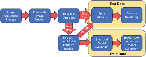
To facilitate reader comprehension, Figure 1 provides a schematic research workflow of the following two sections – Study Area and Data, and Methods.

Figure 1. Schematic of the study’s workflow.

Study area and data

LiDAR bathymetric data

The study area for this work is a 5 km-by-5.5 km area (Figure 2) located to the immediate north of Key West, Florida (United States). The area covers a range of depths, water turbidity, and geomorphology. It also includes areas of land – something that is typical of areas to which SDB techniques are applied to map shallow-water bathymetry. Available for the area was a 2019 green laser (532 nm) airborne LiDAR survey commissioned by the United States National Oceanic and Atmospheric Administration (NOAA). The survey was registered to the UTM projection/coordinate system (Zone 17) as were the Sentinel images employed (as described below.) Data were acquired January 4 and 13, and March 2 in boustrophedonic swaths generally oriented north-south using three circular scanning systems: Riegl™ VQ-880-GII, Riegl™ VQ-880-GH, and Riegl™ VQ-880-G+. The nominal altitude (400 m above mean sea level (MSL)), scan angle (20°) and pulse frequency provided an average spatial density of 10 soundings sq m⁻¹ although this varied across the area; it was notably higher where swaths overlapped. The data were post-processed using NOAA standard operating procedures (SOPS) that entail a combination of automated and manual/human procedures.

Figure 2. The study area showing the locations (red) of 500m-by-500m tile centers (Google Earth™ imagery).

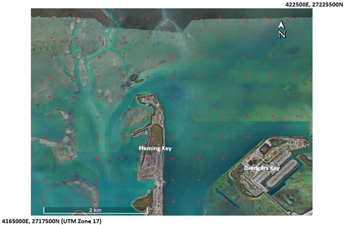
This produced a set of 500-m-by-500 m data tiles registered to the Universal Transverse Mercator (UTM) projection. The easting and northing for the northwest corner of each tile was used as a tile identifier. The study area comprises a rectangle of 110 tiles − 11 tiles east-west by 10 tiles north-south. NOAA SOPs classified each LiDAR sounding as bathymetry (“Bathy”), land/ground, noise, or uncertain. For the purposes of this study, soundings classified by NOAA’s SOPs as Bathy were used as bathymetric/depth reference data – i.e. “truth.” These were tide-corrected to MSL.

Satellite imagery and pixel depth

For satellite imagery, Sentinel-2 (ESA (European Space Agency) 2023) data were employed due to their high spatial and spectral resolution and the relatively high revisit rate of the two Sentinel-2 satellites (2 to 3 days at mid-latitudes). Only four of the 13 available spectral bands – the three visible (Bands 2, 3, 4: blue, green, red) bands and one near infra-red band (Band 8) – are collected at the highest spatial resolution of 10 m. The remaining nine bands are collected in pixels varying from 20 to 60 m. The images were provided by the European Space Agency having been re-sampled to 10 m resolution using a bilinear interpolation method.¹ Four Sentinel-2 images that were cloud-free for the study area and collected as close as possible to January–March 2019 were identified and obtained; the four images were dated (yyyy/mm/dd) 2021/04/13, 2021/05/08, 2021/07/07, and 2022/09/30. These were atmospherically corrected using ACOLITE (RBINS 2023).

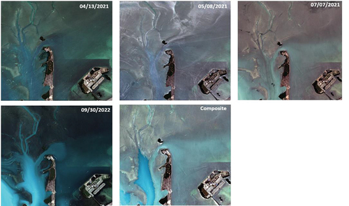
An additional image termed herein the “Composite” was produced from the four images. For each 10 m pixel, as has been done in other studies (e.g., Thomas et al. 2021), the image having the highest reflectance value for Band 2 (blue/490 nm) was determined under the assumption that the highest value for a given band and pixel across all images is indicative of the strongest signal/best data acquisition conditions. For each pixel, the reflectance values for all bands for the image identified as having the highest Band 2 reflectance were assigned to the pixel in the Composite image. Figure 3 shows the date associated with each pixel value and the legend shows the percent of pixels from each image present in the Composite. Notably, the 2021/04/13 image contributed the fewest pixels (2%) to the Composite image. Moreover, these 2021/04/13 pixels were primarily on land areas that were eliminated from subsequent SDB analysis meaning that the 2021/04/13 made virtually no contribution to SDB models that were subsequently developed from the Composite image. Images from the four dates and the composite are shown in Figure 4.

Figure 3. Contribution of individual images to the composite image.

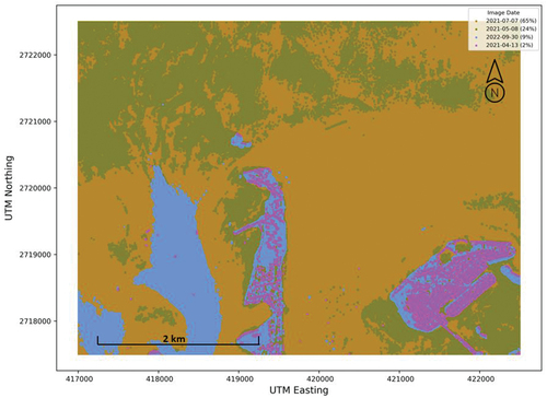
Figure 4. The images from each date and the composite image. Images are displayed as near real color (i.e. Sentinel bands 4, 3, 2 displayed in red, green, and blue, respectively). An image-specific percent clip stretch has been applied to each image.

For all images, to decrease the influence of aberrant pixels, a 3-by-3 median filter was applied.

The reference/”true” depth of each pixel was determined as the median depth (corrected to MSL) of a pixel’s LiDAR soundings identified as Bathy by NOAA SOPs. Pixels whose median was calculated from 10 or fewer soundings were eliminated from subsequent SDB analysis.

Data splitting

To evaluate overfitting subsequently, tiles were split randomly into two groups: train (80%/88 tiles/182,970 pixels) and test (20%/22 tiles/42389 pixels). This split was done on entire tiles rather than individual pixels because a tile-based split is more representative of in situ data availability where SDB techniques are likely to be employed. Specifically, SDB techniques are employed to fill in spatial gaps where in situ reference/ground-“truth” data are completely lacking, rather than in areas where in situ data are available but sparse as would be represented by randomly sampling individual pixels.

Methods

One goal of this work was to evaluate the comparative accuracy of quasi-empirical SDB models with that of ML models including the ability of both types to produce geographically adaptive models. For example, Figure 2 suggests the potential need for three models due to image characteristics, geomorphology, or some other unknown cause(s): one for the northern (and southeastern) area (green in Figure 2), one for the southwestern area (blue), and one for the remaining area (orange). Yet fitting separate models for these areas would ignore the intra-area intermixing of pixels from different images and also runs the risk of creating seams of large depth differences where different models would be applied. Hence the potential for geographically adaptable models was accommodated simply by making available to the model fitting procedure the UTM easting and northing of each pixel.

Quasi-empirical models

A widely used (e.g., Evagorou et al. 2022; Hsu et al. 2021) quasi-empirical SDB model employed was first described by Stumpf et al. (2003):

(1) $Depth=\frac{m_1\ast ln\left(k\ast B\right)}{ln\left(k\ast G\right)}+m_0$(1)

where m₀ and m₁ are regression coefficients, k is a constant usually set to 1000 as was the case here to ensure that both logarithms are always positive and that a residual non-linearity is removed (Caballero and Stumpf 2020b) and B and G are the reflectances in the blue and green satellite bands, respectively – Bands 2 and 3 for Sentinel-2. Because this is a linear model that has a closed-form solution, making it geographically adaptive requires the inclusion of UTM eastings and northings as well as explicit definition of interactions. Hence, this SDB model was fitted as presented in Equation (1)(1) $Depth=\frac{m_1\ast ln\left(k\ast B\right)}{ln\left(k\ast G\right)}+m_0$(1) , and also with the inclusion of UTM eastings and northings and all multiplicative 2-way interactions and the single possible 3-way interaction [easting*northing*ln(k*Blue)/ln(k*Green)]. To be able to compare the contributions of variables to the Equation (1)(1) $Depth=\frac{m_1\ast ln\left(k\ast B\right)}{ln\left(k\ast G\right)}+m_0$(1) model in a way that was consistent with “variable importance” inherent in the ML method selected (see next paragraph), the Student’s t-distribution values associated with the coefficients of each variable (a standard output of linear regression) were normalized to sum to 100 over all variables. The t values for interaction variables – e.g., easting*northing – were split equally between individual component variables before normalization.

Machine learning (ML) models

For the ML model, it is noted that the goal of this work was not to identify the best ML method from a number of ML methods. Instead, one goal of this work was to evaluate a representative empirical method that provides for the inclusion of a large number of Sentinel bands and UTM coordinates, and whose relationship(s) to depth and each other is unknown. It was also desired to be able to readily evaluate the contribution of each variable to model accuracy. The empirical modeling methodology selected was Categorical Boosting (“CatBoost;” Prokhorenkova et al. 2018) – a ML decision tree-based approach. Decision trees progressively split data in two based on a variable and its value that will have the greatest impact on model accuracy at a given split. The number of splits performed is user-controlled or determined by an analytical criterion such as statistical significance or numeric optimality. The CatBoost method has been shown to perform somewhat better than often-employed extreme gradient boosting (XGB; Chen and Guestrin 2016) and LightGBM (Ke et al. 2018). Originally formulated to better accommodate categorical data (something that is not a consideration in this work), CatBoost also introduces “ordered boosting” that builds on existing models/trees to develop subsequent trees. As with other decision-tree methods, it produces a single final decision-tree model by combining the shallow decision trees developed. It implicitly accommodates unknown interactions, as well as non-linear relationships. A variable’s importance is determined by the number of trees in which it appears with importance values being normalized across all variables so that the total importance is 100.

Hence, six models were fitted for each image (Table 1). The inclusion of Bands 1, 5, and 11 in Models 5 and 6 resulted from exploratory model fitting that suggested these bands had the potential to improve CatBoost SDB models substantially despite, for example, an a priori expectation that infrared bands (5 and 11) would provide no water penetration and therefore not be indicative of bathymetric depth. It is acknowledged that others have suggested that Band 1 is superfluous to Band 2 because of high collinearity between the two (Casal et al. 2019). However, the finding of the a priori variable exploration conducted was consistent with Thomas et al. (2021) who determined that the inclusion of Band 1 improved the accuracy of a multiple linear regression SDB model.

Table 1. Models explored.

Model	Method	Description	Geographically Adaptive	Bands/Variables
1	Linear Regression	Quasi-empirical (Equation (1)(1) $Depth=\frac{m_1\ast ln\left(k\ast B\right)}{ln\left(k\ast G\right)}+m_0$(1) )	No	$Bandratio\left(BR\right):\frac{ln\left(1000\ast Blue\right)}{ln\left(1000\ast Green\right)}$
2			Yes	BR, Easting, Northing, BR*Easting, BR*Northing, Easting*Northing, BR*Easting*Northing
3	CatBoost	Visible Sentinel-2 bands	No	2 (Blue), 3 (Green), 4 (Red)
4			Yes	2, 3, 4, Easting, Northing
5		Visible bands plus other selected bands^1	No	2, 3, 4, 1 (“ultra blue”), 5 (visible and near infrared), Band 11 (short-wave infrared)
6			Yes	2, 3, 4, 1 (“ultra blue”), 5 (visible and near infrared), Band 11 (short-wave infrared), Easting, Northing

¹“Other” bands were selected based on a priori exploratory model fitting.

Model fitting and evaluation

All six models were fitted for each of the five images using the pixel data from the 88 training tiles (182,970 pixels) – i.e. 30 models total were produced. R-squared values and the root mean square error (RMSE in m) were used to evaluate differences among images and models including the impact of UTM eastings and northings. Models developed for a particular image were then applied to all pixels in that image including those on the 22 test tiles (42,389 pixels) to produce an SDB depth estimate for each pixel on that image. For each model-image-test/train combination, a linear regression was fitted between the reference/ground-“truth” data as the independent x variable and the SDB depth estimate as the dependent y variable for individual pixels. These are subsequently referred to as “uncertainty regressions.” For a tile with unbiased low uncertainty/high predictive accuracy, the intercept and slope of its uncertainty regression will be 0.0 and 1.0, respectively, and the r-squared will be “high” and the RMSE “low.” Moreover, if the SDB model that generated the depth estimate is not overfitted, values for these four metrics will be similar for the train and test data sets. This was examined globally for each image.

The importance of variables was examined. Of particular interest was the relative importance of UTM eastings and northings in the models that included them – i.e., the geographically adaptive models. Also of considerable interest was the relative importance of non-visible spectral bands (1, 5, and 11) in the two models in which they appeared.

To examine error structure spatially, the uncertainty regressions were fitted for each of the 110 tiles. The local spatial structure of uncertainty was examined by calculating the spatial autocorrelation metric Moran’s I globally (Odland 1988) and locally (Anselin 1995) for the r-squared values and RMSE values for the uncertainty regressions for each tile.

Globally and locally I varies from −1.0 to 1.0 with negative values indicating a tendency for interspersion of high and low (r-squared or RMSE) values (like a chess board), and positive values indicating an unusual spatial clustering of high or low values; an I value near zero suggests a spatially random distribution of values. A statistically significant value for global I indicates a significant deviation from a random spatial pattern over an entire area – unusual interspersion (negative I) or clustering (positive I). For local application, an I value is calculated for each spatial unit (tile) based on a unit’s “neighbours” as defined by distance or adjacency; adjacency was used in this study. Monte-Carlo simulation is used to develop frequency distributions that provide for significance testing. The result is that statistically significant local “hotspots” can be identified. Importantly, however, a statistically significant positive local I (hotspot) indicates significant clustering, but it does not indicate if the clustering is among high or low (depth) values. Similarly, a significant negative local I value indicates unusually high localized variation of (depth) values. To determine if a hotspot indicates clustering of high or low (r-squared or RMSE) values, the local I scatterplot and associated quadrant analysis (Anselin 1996) can be undertaken for all significant (95% confidence) hotspots having positive I values. This was done in this study.

Results

Statistical model evaluation

Figure 5 indicates clearly that the empirical CatBoost models outperformed the quasi-empirical linear regression model (Equation (1)(1) $Depth=\frac{m_1\ast ln\left(k\ast B\right)}{ln\left(k\ast G\right)}+m_0$(1) ): for all image dates r-squared values were considerably lower, and RMSE values considerably higher for the Stumpf model/Equation (1)(1) $Depth=\frac{m_1\ast ln\left(k\ast B\right)}{ln\left(k\ast G\right)}+m_0$(1) than for any of the CatBoost ML models for the pixels on the training tiles. Also apparent is that providing the capacity for models to be geographically adaptive by including UTM eastings and northings improved all models. For model pairs (i.e., Models 1 and 2, Models 3 and 4, Models 5 and 6), “with-UTM” models produced higher r-squared values and lower RMSE values than their related “without-UTM” model for the pixels on the training tiles. The CatBoost models that included non-visible spectral bands − 1 (ultra-blue), 5 (near infrared) and 11(short wave infrared) – outperformed the CatBoost models containing only the visible bands − 2, (blue), 3 (green), and 4 (red). Interestingly, the CatBoost model with visible bands alone plus UTM coordinates (Model 4²) (purple bars in Figure 5) performed slightly better than the CatBoost model containing the non-visible bands plus the UTM coordinates (pink bars in Figure 5) for all images except 2021/05/08. However, the CatBoost model containing visible and non-visible bands plus UTM coordinates (Model 6) clearly performed best indicating that 1) the non-visible Sentinel bands employed make an important contribution to model accuracy and 2) the inclusion of UTM coordinates is a relatively simple way of improving model accuracy by making models geographically adaptive.

Figure 5. (a) Average r-squared and (b) root mean square error (m) by model type (see Table 1) and image date for training data.

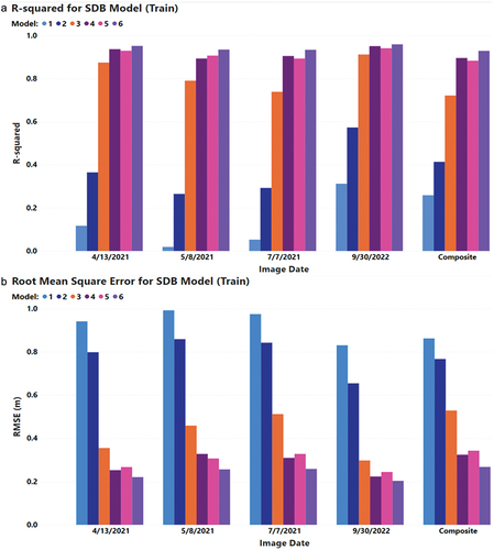
To assess the models for different images, because the quasi-empirical models (Models 1 and 2) performed clearly worst, only the CatBoost models that included visible and non-visible bands and UTM coordinates (Model 6) are considered. Interestingly, this indicates that the two images that contributed the least to the composite image (Figure 3: 2022/04/13 and 2022/09/30) produced the best SDB models for the training data; r-squared values are highest and RMSE values the lowest for these images. It is noted, however, that the r-squared and RMSE values for all images are comparable. This indicates that when using CatBoost to fit a purely empirical model using Sentinel-2 data, image selection and/or compositing multiple images is relatively unimportant provided a geographically adaptive model that employs Bands 1, 2, 3, 4, 5, and 11 is fitted. By extension, it is likely that the same would be true of other tree-based ML model fitting approaches. Finally, it is speculated that the CatBoost models (Models 3 to 6) far outperformed the quasi-empirical models (Models 1 and 2) because of their ability to identify and employ “hidden” interactions and local tendencies. This is supported by the differences in quasi-empirical model performance for different images. This further suggests that whereas image selection or compositing is of minor concern when using CatBoost modeling (or presumably other machine learning methods), these may be quite important when using linear modeling techniques such as regression.

Variable importance

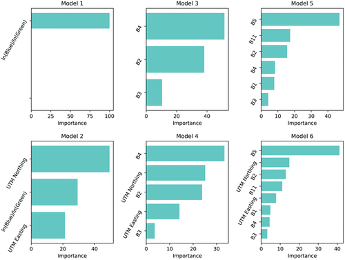
Figure 6 shows the relative importance of variables in the SDB models; the top row shows results for the SDB models that did not include UTM coordinates (Models 1, 3, and 5) and the bottom row shows results for the SDB models that did include the UTM coordinates (Models 2, 4, and 6). In the models that did include the UTM coordinates (bottom row), the UTM northing was consistently more important than the UTM easting. Moreover, the UTM northing was one of the two most important variables. This is undoubtedly related to the shallow area of seagrass that exists across the northern portion of the area (Figure 1) which was also reflected in the contribution of each image to the composite image (Figure 2). The UTM easting also appeared to make a useful contribution to the SDB CatBoost models; this is probably related to the area having deeper channels in the southwest (also reflected in a dominant contribution from the image dated 2022/09/30 to the Composite image; Figure 2). Also of interest is that in the CatBoost models that included visible and non-visible bands, it was the near-infrared Band 5 that was most important, with the non-visible short-wave infrared Band 11 being similarly important. This is somewhat surprising given that bands in the infrared portion of the spectrum have little or no water penetration capability. Moreover, that Bands 5 and 11 were captured at 20 m and re-sampled to 10 m does not appear to have had an impact on their importance. The most important visible band was Band 2 (blue).

Figure 6. Relative importance of variables over all images. See Table 1 for model definitions. Top row models are not geographically adaptive; bottom row is geographically adaptive equivalent of the model above it.

Overfitting assessment

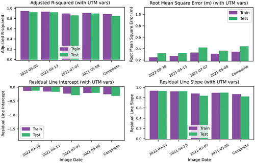
Figure 7 presents information that can be used to evaluate potential overfitting for the model most likely to be overfitted by virtue of having the most variables – the geographically adaptive CatBoost model that employs visible and non-visible spectral bands (Model 6). It does not appear that this SDB model is overfitted. Adjusted r-squared values and RMSE values for uncertainty regressions fitted on training data are only slightly better (higher r-squared and lower RMSE values) than those fitted on test data. Similarly, the slopes and intercepts of the uncertainty regression lines are similar for the training and test data. Comparable results were observed for all images and models. Recall, however, that an ideal model fit for the uncertainty regression lines would have a slope of 1.0 and intercept of 0.0 – i.e. reference/”true” depth would be equal to the SDB model prediction. A slope less than 1.0 and negative intercept indicates that for both training and test data, shallow depths are overestimated (i.e. estimated depths are “too deep”) and larger depths are underestimated (i.e. estimated depths are “too shallow”). This occurred for all images for all SDB models. One possible reason is that even the flexibility to model non-linear relationships that CatBoost provides is not sufficient for the area examined and the data employed. It is conceivable, for example, that the visible-near infrared Band 5 had its unexpected high importance because there is some penetration in very shallow areas, but the penetration decreased relatively rapidly, and in a non-linear manner as depth increased.

Figure 7. Evaluation of model overfitting for each image for the CatBoost model based on bands 1, 2, 3, 4, 5, and 11 and UTM northing and easting.

Spatial model evaluation

It was expected that a clustered spatial structure for model uncertainty would be present with uncertainty being related to a positively spatially autocorrelated characteristic such as substrate, or water depth or clarity. In fact, however, for none of the 30 model/image combinations did Moran’s I manifest a statistically significant value (α = 0.05; p ranged from 0.10 to 0.97 for r-squared and from 0.09 to 0.99 for RMSE). Figure 8 shows an example surface for both r-squared and RMSE for the best model and image combination (Model 6: geographically adaptable model for CatBoost with visible and non-visible bands for the image dated 2022/09/30).

Figure 8. Example surfaces showing r-squared values (a.) and RMSE values (b.) for the CatBoost model fitted using and bands 1, 2, 3, 4, 5, and 11 and UTM northing and easting for the 2022/09/30 image. (For r-squared (a.), Moran’s I/p is 0.07/0.10, and −0.02/0.89 for RMSE (b.). Tiles with gray “haloes” comprise the test data set. Dots indicate a statistically significant (α = 0.05) cluster of values with pink indicating (a.)high r-squared)/(b.)low RMSE values (i.e. desirable model performance) and olive indicating (a.)low r-squared/(b.)high RMSE values (i.e. undesirable model performance).

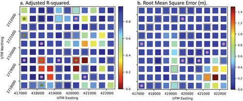
Present on Figure 8 are dots indicating areas of significant (α = 0.05) clustering of values; areas with significant interspersion of high/low values are not displayed and were ignored. On Figure 8, pink dots indicate areas of desirable model performance and olive dots indicate areas of undesirable model performance. (Also indicated by gray “haloes” around tiles are the tiles whose pixels comprised the test data set.) Across all 30 model-image combinations, the number of pink (desirable) hotspots for r-squared ranged from 0 to 9 and for RMSE from 0 to 7; the range of olive (undesirable) hotspots ranged from 0 to 7 for R² and from 2 to 8 for RMSE. Readers are reminded that with α = 0.05 and 110 tiles present, it is expected that 5.5 hotspots (i.e., approximately three hotspots indicating significant clustering of high or low values and three indicating significant dispersion) will manifest as statistically significant by chance. Hence, to better understand if there are areas where high or low values “truly” cluster, the number of pink (desirable model accuracy) and olive (undesirable model accuracy) hotspots were accumulated across all five images (Figure 9).

Figure 9. The number of image-model combinations on which each tile was a significant (α = 0.05) hotspot indicating desirable model performance (a. and c.) or undesirable model performance (b. And d.). Gray tiles are those that were never hotspots. Tiles with gray “haloes” comprise the test data set.

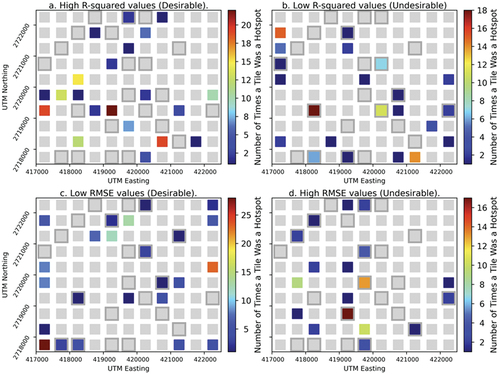
Recall that there are a total of (5 images × 6 models = 30 image-model combinations). There are relatively few tiles out of the 110 on the study area for which models were consistently accurate or inaccurate; these are the tiles having “hotter” colors in Figure 9. It was expected a priori that accuracy for certain tiles across all image-model combinations would be consistently desirable/undesirable reflecting, for example, optimal geomorphology (desirable) or consistently turbid water (undesirable). And there are, in fact, a number of the 110 tiles whose accuracy was consistently desirable or undesirable – i.e., those with the “hotter” colors in Figure 9. However, it was also expected that tiles with desirable/undesirable image-model combinations would tend to cluster spatially. Instead, tiles for which image-model combinations were most consistently desirable or undesirable hotspots tended to be spatially dispersed. Somewhat complicating this observation is that r-squared values that showed good model performance tended to not be those whose RMSE also showed good model performance. The same was true of tiles indicating poor model performance. Arguably, the area in the northeast of the study area showed the most consistent result over all image-model combinations – no tiles identified as consistently desirable/undesirable hotspots were present with the exception of a few tiles for RMSE for good image-model performance. This suggests that errors associated with bathymetric maps will be spatially random at a spatial resolution of 500 km. Further work would be necessary to discern causes/general tendencies in image-model combinations.

The data on which Figure 9 is based provide a means of assessing relative performance/accuracy of image-model combinations on the training and test data sets. The number of 95% desirable and undesirable hotspots for the r-squared and RMSE metrics for the training and test data sets were summed over all image-model combinations and converted to a percentage of total hotspots. If the model-image combinations are generally the same for training and test data sets, it is expected that the training/test split of hotspots would be 80%/20% since these are the percentages of tiles in the training and test data sets, respectively. Table 2 suggests a mixed result. For example, 99% of the desirable hotspots for r-squared were present on training tiles (far more than the 80% expected), but 62% of the desirable hotspots for RMSE were on test tiles (far more than the 20% expected). This does not appear to be a result of model overfitting. Figure 7 suggests that the amount of model overfitting (on the training data) was minimal for the most complex model across all images. And visual examination of graphics suggested that the level of overfitting was comparable for the other less complex models.

Table 2. Percentage of desirable and undesirable hotspots for the training and test data sets over all images. Green cells indicate a higher percentage than expected based on the 80/20 train/test data split; red cells indicate a lower percentage.

Discussion and conclusions

A relatively common strategy in developing bathymetric depth maps using SDB techniques is to develop a composite image from multiple cloud-free maps. In the work presented, such a composite did not produce the best SDB models and accuracy metrics compared to the (four) individual images used to create the composite. Moreover, only 9% of the composite image comprised pixels from the individual image that produced the best SDB bathymetric map (2022/09/30). It is thus clear that under some conditions, image compositing is not the optimal strategy for developing an image that is used for SDB. A better alternative strategy may be to produce SDB using each “candidate image” potentially including a composite image and select the optimal image/SDB model a posteriori.

The pixels comprising the composite image generally appeared in large cohesive areas (Figure 2) that reflected areas that were recognizably different (Figure 3). That the composite image on which these different areas are recognizable did not produce the best SDB bathymetric maps is indicative that compositing is not necessarily the optimal strategy for capturing these differences. However, the inclusion of geographic coordinates – UTM eastings and northings – and the use of a tree-based ML approach produced geographically adaptive SDB models from individual images that performed better than models that were not geographically adaptive. Moreover, the geographically adaptive ML models performed better than a widely used quasi-empirical linear regression model that was made geographically adaptive. It is thus concluded that tree-based ML methods have the capacity and flexibility to accommodate unknown and potentially non-linear relationships and interactions among geographic tendencies, spectral reflectance, and water depth in the production of SDB maps.

Much SDB work that employs Sentinel-2 imagery confines itself to the visible bands − 2 (blue), 3 (green), and 4 (red) (e.g., Pahlevan et al. 2017). This is reasonable as these bands are captured at a 10 m spatial resolution and these visible bands have a physically definable relationship with shallow-water depth. However, the work described clearly demonstrated that models that included non-visible (including infrared) bands captured at coarser spatial resolutions and re-sampled to 10 m using bilinear interpolation produced better SDB models and maps than those that confined themselves to the use of high spatial resolution visible bands only. Perhaps most notable was Band 1 (ultra blue) that is captured at a 60 m resolution. Its importance after being re-sampled to 10 m was low (Figure 4, Models 5 and 6), but not as low as Band 3 (green) that was captured (not re-sampled) at a 10 m resolution. This suggests that the Band 1 wavelength can be useful for depth estimation, even if the bilinear interpolation process degrades the signal or adds noise. Given the “black boxy” nature of the CatBoost modeling technique, however, it is not possible to characterize the nature of the relationship meaning that its successful use in such work may be reliant on a machine learning modeling methodology.

This result highlights both a strength and a weakness of machine learning decision trees as a modeling methodology. As surmised in the Results section, it is possible that Band 5 visible/near-infrared has a not-previously-known non-linear relationship with depth in shallow areas that can only be detected by a highly flexible machine learning modeling technique. However, such a relationship may be local only thereby limiting the applicability of the model and its extension to other data and areas. Hence, the unexpected high importance of Band 5 considerably improved the modeling of SDB for the study area and data employed in this study, but the result may not be generalizable to other areas and data.

Spatial analysis of the SDB model/map (in)accuracy indicates that local accuracy will vary widely for SDB maps. For example, Figure 8 shows that for the best image and model, RMSE can vary by as much as 1.4 m across an area. Moreover, the global spatial autocorrelation coefficient Moran’s I indicates that the pattern of (in)accuracy is spatially random. Nonetheless, Figure 9 demonstrates that accuracy is consistently poor for certain areas regardless of model type or image employed. These results show a clear need for more research to better characterize inaccuracy associated with SDB models/techniques. It is acknowledged that such findings may be of limited interest/concern for uses of SDB maps focused on areas larger than 500 m tiles. However, for uses such as navigation in which local accuracy is critical, the results presented suggest a clear need for caution in the use of SDB products based on global statements of accuracy.

This research has demonstrated a number of important points about uncertainty associated with SDB models – e.g., its magnitude, its globally and locally random spatial pattern – as well as the nature of model fitting using machine learning techniques. An overarching final point of interest is the broader applicability of the techniques and findings. While the model fitting and evaluation techniques are undoubtedly extensible to other data sets and areas, it is not clear that the results would be comparable. In fact, it was somewhat surprising to the authors that global uncertainty did not manifest a clustered pattern – i.e., significant positive global spatial autocorrelation – given that relatively shallow seagrass is clustered in the northwest portion of the study area (see Figure 2). Other areas with comparable clustered phenomena – e.g., turbid water where a river empties into a bay – may show a nonrandom pattern of uncertainty. Similarly, the magnitude of uncertainty may vary in such areas with a high relation to the satellite imagery used, the ocean substrate, water clarity, and other factors. Such observations reinforce the need for a statistically and spatially robust analysis of model uncertainty when SDB techniques are used to estimate water depth.

Acknowledgments

This work was supported by the National Oceanic and Atmospheric Administration (NOAA) Grant NA15NOS400020. We appreciate the comments of three anonymous individuals whose reviews have helped improve this article.

Data availability statement

Data supporting this study are available at https://doi.org/10.6084/m9.figshare.23631549.

Disclosure statement

No potential conflict of interest was reported by the authors.

Additional information

Funding

This work was supported by the NOAA Research [NA15NOS400020].

Notes

1. https://sentinels.copernicus.eu/web/sentinel/technical-guides/sentinel-2-msi/level-1c/algorithm-overview Current as of November 2023.

2. See Methods section for definition of models.

References

- Anselin, L. 1995. “Local Indicators of Spatial Association – LISA.” Geographical Analysis 27 (2): 93–15. https://doi.org/10.1111/j.1538-4632.1995.tb00338.x.
- Anselin, L. 1996. “The Moran Scatterplot as an ESDA Tool to Assess Local Instability in Spatial Association.” In Spatial Analytical Perspectives on GIS, edited by M. Fischer, H. Scholten, and D. Unwin, 111–125. London: Taylor & Francis.
- Brando, V., J. Anstee, M. Wettl, A. Dekker, S. Phinn, and C. Roelfsema. 2009. “A Physics-Based Retrieval and Quality Assessment of Bathymetry from Suboptimal Hyperspectral Data.” Remote Sensing of Environment 113 (4): 755–770. https://doi.org/10.1016/j.rse.2008.12.003.
- Caballero, I., and R. Stumpf. 2020a. “Atmospheric Correction for Satellite-Derived Bathymetry in the Caribbean Waters: From a Single Image to Multi-Temporal Approaches Using Sentinel-2A/B.” Optics Express 28 (8): 11742–11766. https://doi.org/10.1364/OE.390316.
- Caballero, I., and R. Stumpf. 2020b. “Towards Routine Mapping of Shallow Bathymetry in Environments with Variable Turbidity: Contribution of Sentinel-2A/B Satellites Mission.” Remote Sensing 12 (3): 451–11766. https://doi.org/10.3390/rs12030451.
- Cahalane, C., A. Magee, X. Monteys, G. Casal, J. Hanafin, and P. Harris. 2019. “A Comparison of Landsat 8, RapidEye and Pleiades Products for Improving Empirical Predictions of Satellite-Derived Bathymetry.” Remote Sensing of Environment 233 (111414): 15. https://doi.org/10.1016/j.rse.2019.111414.
- Casal, G., J. Hedley, X. Monteys, P. Harris, C. Cahalane, and T. McCarthy. 2020. “Satellite-Derived Bathymetry in Optically Complex Waters Using a Model Inversion Approach and Sentinel-2 Data.” Estuarine, Coastal and Shelf Science 241 (106814): 15. https://doi.org/10.1016/j.ecss.2020.106814.
- Casal, G., X. Monteys, J. Hedley, P. Harris, C. Cahalane, and T. McCarthy. 2019. “Assessment of Empirical Algorithms for Bathymetry Extraction Using Sentinel-2 Data.” International Journal of Remote Sensing 40 (8): 2855–2879. https://doi.org/10.1080/01431161.2018.1533660.
- Chen, T., and C. Guestrin, 2016. “XGBoost: a scalable tree boosting system,” Knowledge Discovery and Data Mining Conference (KDD 16), San Francisco, California, United States, 785–794. https://doi.org/10.1145/2939672.2939785.
- Chu, S., L. Cheng, X. Ruan, Q. Zhuang, X. Zhou, M. Li, and Y. Shi. 2019. “Technical Framework for Shallow-Water Bathymetry with High Reliability and No Missing Data Based on Time-Series Sentinel-2 Images.” IEEE Transactions on Geoscience & Remote Sensing 57 (11): 8745–8763. https://doi.org/10.1109/TGRS.2019.2922724.
- ESA (European Space Agency), “Sentinel-2 MSI User Guide”. Accessed July, 2023. https://sentinels.copernicus.eu/web/sentinel/user-guides/sentinel-2-msi.
- Evagorou, E., A. Argyriou, N. Papadopoulos, C. Mettas, G. Alexandrakis, and D. Hadjimitsis. 2022. “Evaluation of Satellite-Derived Bathymetry from High and Medium-Resolution Sensors Using Empirical Methods.” Remote Sensing 14 (3): 20. DOI. https://doi.org/10.3390/rs14030772.
- Hsu, H.-J., C.-Y. Huang, M. Jasinski, Y. Li, H. Gao, T. Yamanokuchi, C.-G. Wang, et al. 2021. “A Semi-Empirical Scheme for Bathymetric Mapping in Shallow Water by ICESat-2 and Sentinel-2: A Case Study in the South China Sea.” ISPRS Journal of Photogrammetry & Remote Sensing 178:1–19. https://doi.org/10.1016/j.isprsjprs.2021.05.012.
- Ke, G., Q. Meng, T. Finley, T. Wang, W. Chen, W. Ma, Q. Ye, and T.-Y. Liu, 2018. “LightGbm: A Highly Efficient Gradient Boosting Decision tree,” 31st Conference on Neural Information Processing Systems (NeurIPS 2018), Long Beach, California, United States, 9. Accessed July, 2023. https://proceedings.neurips.cc/paper_files/paper/2017/file/6449f44a102fde848669bdd9eb6b76fa-Paper.pdf.
- Li, S., X. Hua Wang, Y. Ma, and F. Yang. 2023. “Satellite-Derived Bathymetry with Sediment Classification Using ICESat-2 and Multispectral Imagery: Case Studies in the South China Sea and Australia.” Remote Sensing 15 (4): 15. DOI. https://doi.org/10.3390/rs15041026.
- Li, J., D. Knapp, S. Schill, C. Roelfsema, S. Phinn, M. Silman, J. Mascaro, and G. Asner. 2019. ““Adaptive Bathymetry Estimation for Shallow Coastal Waters Using Planet Dove Satellites.” Remote Sensing of Environment 232:111302–111314. https://doi.org/10.1016/j.rse.2019.111302.
- Lyons, M., M. Roelfsema, C. Kennedy, E. Kovacs, R. Borrego-Acevedo, K. Markey, M. Roe, et al. 2020. “Mapping the World’s Coral Reefs Using a Global Multiscale Earth Observation Framework.” Remote Sensing in Ecology and Conservation 6 (4): 557–568. https://doi.org/10.1002/rse2.157.
- Lyzenga, D., N. Malinas, and F. Tanis. 2006. “Multispectral Bathymetry Using a Simple Physically Based Algorithm.” IEEE Transactions on Geoscience & Remote Sensing 44 (8): 2251–2259. https://doi.org/10.1109/TGRS.2006.872909.
- Mishra, M., D. Ganguly, and D. Chauhan. 2013. “Estimation of Coastal bath6mtry Using RISAT 1-C Band Microwave SAR Data.” IEEE Geoscience & Remote Sensing Letters 11 (3): 671–675. https://doi.org/10.1109/LGRS.2013.2274475.
- Misra, A., B. Vojinovic, B. Ramakrishnan, A. Luijendijk, and R. Ranasinghe. 2018. “Shallow Water Bathymetry Mapping Using Support Vector Machine (SVM) Technique and Multispectral Imagery.” International Journal of Remote Sensing 39 (13): 4431–4450. https://doi.org/10.1080/01431161.2017.1421796.
- Odland, J. 1988. Spatial Autocorrelation. London: SAGE Publications Scientific Geography Series, SAGE Publications Inc, 87.
- Pacheco, A., J. Horta, C. Loureiro, and O. Ferreira. 2015. “Retrieval of Nearshore Bathymetry from Landsat 8 Images: A Tool for Coastal Monitoring in Shallow Waters.” Remote Sensing of Environment 159:102–116. https://doi.org/10.1016/j.rse.2014.12.004.
- Pahlevan, N., S. Sarkar, A. Franz, S. Balasubramanian, and J. He. 2017. “Sentinel-2 multispectral instrument (MSI) data processing for aquatic science applications: demonstration and validations.” Remote Sensing of Environment 201:47–56. https://doi.org/10.1016/j.rse.2017.08.033.
- Pereira, P., P. Baptista, T. Cunha, P. Silva, S. Romao, and V. Lafon. 2019. “Estimation of the Nearshore Bathymetry from High Temporal Resolution Sentinel-1A C-Band SAR Data – a Case Study.” Remote Sensing of Environment 223:166–178. https://doi.org/10.1016/j.rse.2019.01.003.
- Poursanidis, D., D. Traganos, N. Chrysoulakis, and P. Reinartz. 2019. “Cubesats Allow High Spatiotemporal Estimates of Satellite-Derived Bathymetry.” Remote Sensing 11 (11): 1299, 12. https://doi.org/10.3390/rs11111299.
- Prokhorenkova, L., G. Gusev, A. Vorobev, A. Dorogush, and A. Gulin, 2018. “CatBoost: Unbiased Boosting with Categorical Features,” 32nd Conference on Neural Information Processing Systems (NeurIPS 2018), Montreal, Quebec, Canada (11 pp). Accessed July , 2023. https://papers.nips.cc/paper_files/paper/2018/file/14491b756b3a51daac41c24863285549-Paper.pdf.
- RBINS (Royal Belgian Institute of Natural Sciences), 2023. ACOLITE. Accessed July , 2023. https://odnature.naturalsciences.be/remsem/software-and-data/acolite.
- Sagawa, T., Y. Yamashita, T. Okumura, and T. Yamanokuchi. 2019. “Satellite Derived Bathymetry Using Machine Learning and Multi-Temporal Satellite Images.” Remote Sensing 11 (10): 1155, 19. DOI. https://doi.org/10.3390/rs11101155.
- Stumpf, R., K. Holderied, and M. Sinclair. 2003. “Determination of Water Depth with High-Resolution Satellite Imagery Over Variable Bottom Types.” Limnology & Oceanography 48 (1): 547–556. Part 2: Light in Shallow Waters. https://doi.org/10.4319/lo.2003.48.1_part_2.0547.
- Thomas, N., A. Pertiwi, D. Traganos, D. Lagomasino, D. Poursanidis, S. Moreno, and L. Fatoyinbo. 2021. “Space-Borne Cloud-Native Satellite-Derived Bathymetry (SDB) Models Using ICESat-2 and Sentinel-2.” Geophysical Research Letters 48 (6): 11. https://doi.org/10.1029/2020GL092170.
- Traganos, D., D. Poursanidis, B. Aggarwal, N. Chrysoulakis, and P. Reinartz. 2018. “Estimating Satellite-Derived Bathymetry (SDB) with the Google Earth Engine and Sentinel-2.” Remote Sensing 10 (6): 18. https://doi.org/10.3390/rs10060859.
- Van an, N., N. Hao Quang, T. Hoang Son, and T. An. 2023. “High-Resolution Benthic Habitat Mapping from Machine Learning on PlanetScope Imagery and ICESat-2 Data.” Geocarto International 38 (1): 2184875. https://doi.org/10.1080/10106049.2023.2184875.
- Xu, N., X. Ma, Y. Ma, P. Zhao, J. Wang, and X. Wang. 2021. “Deriving Highly Accurate Shallow Water Bathymetry from Sentinel-2 and ICESat-2 Datasets by a Multitemporal Stacking Method.” IEEE Journal O Selected Topics in Applied Earth Observation and Remote Sensing 14:6677–6685. https://doi.org/10.1109/JSTARS.2021.3090792.