Characterization of north Greenland polynyas with super-resolved passive microwave sea ice concentration

ABSTRACT

Located at the easternmost sector of the Last Ice Area (LIA) with the oldest and thickest sea ice, the north of Greenland has witnessed some unprecedented polynyas since 2018, receiving considerable attention. Sea ice concentration (SIC) derived from passive microwave data can provide near daily observations of these polynyas. However, these SIC products are limited by the coarse spatial resolution of passive microwave data, with mixed pixels and large uncertainties at the ice–water divide. It is especially difficult in the case of newly formed polynyas in the form of leads with narrow openings, preventing accurate estimation of the regional energy budget and heat fluxes as well as the hindering causal analysis of the polynyas. In this paper, a novel state-of-the-art deep-learning-based super-resolution (SR) method is adopted, and passive microwave SR images, with spatial resolutions of up to 4 times the original, are generated and employed to derive super-resolved SIC (SR-SIC). Experimental results confirm the benefits of SR-SIC for finer monitoring of sea ice at both the polynya and lead scale compared to the original lower-resolution SIC, with an average 7.55% improvement in F1-Score for polynya extent and 31.17% for lead width. Using the SR-SIC, more accurate quantitative parameters of polynyas and leads are extracted to present more detailed spatial distributions at their different development stages. For example, SR-SIC with reduced mixed pixels can distinguish more SIC values below 40%, advantageous for detecting open water pixels within polynya areas and improving the accuracy of heat fluxes estimation and ice production calculation. Moreover, SR-SIC has the capability to identify leads with openings less than 3 km and to locate the finer boundaries of the polynyas. Finally, it is found that the lead development along the 2018 winter polynya is associated with regional wind, air temperature, and ice drift. The prominent summer polynya events in 2018, 2020, and 2021 may be in part caused by the thinning sea ice in the north of Greenland.

KEYWORDS:

• Polynya
• lead
• sea ice concentration
• super resolution
• passive microwave data

1. Introduction

Artic sea ice is a sensitive indicator of global climate change, controlling the ice–ocean–atmosphere balance of heat, mass, and momentum, with important impacts on regional ecosystems (Brown et al. 2014; Ding et al. 2019; Liu et al. 2020; Romanov 2017). Recent studies have shown that Arctic sea ice is experiencing a continuous decline, as well as becoming thinner and younger, resulting in its susceptibility to atmospheric winds and in increased mobility. These changes then further promote the occurrence of sea ice fragmentation and important sea ice surface phenomena, such as the opening of leads and polynyas (Moore, Howell, and Brady 2021; Murashkin et al. 2018; Peng, Matthews, and Yu 2018). The occurrence of leads and polynyas plays an important role in regional energy budget and climate change, since leads and polynyas are responsible for about half of the atmosphere–ocean heat exchange in the Arctic in winter (Lee et al. 2023; Qu et al. 2019; Zhang et al. 2018).

The oldest and thickest ice zone, the Last Ice Area (LIA), is located within the region between the Canadian Arctic Archipelago, Greenland, and the North Pole, which climate models predict will be the last area in the Arctic to lose its sea ice (Newton et al. 2021; Schweiger et al. 2021). However, it has also been observed that sea ice in the LIA has been more dynamic than in the past (Moore et al. 2019). A sign of rapid change in the LIA occurred in February 2018, when satellite imagery observed the formation of an unusual winter polynya off the northern coast of Greenland, lasting from February 14 to March 8, with a maximum area of more than 60,000 km² (Ludwig et al. 2019). Afterward, some pronounced polynyas were observed again in the same area in August starting in 2018. The occurrence of these polynya events is of great significance and warrants considerable attention, since they are located in the LIA. This is especially the case for the 2018 winter polynya, the largest and longest-lasting polynya event observed in the region in winter since 1979, when sea ice concentration (SIC) observation records, through remote sensors began. It can thus be considered an extreme event (Moore et al. 2018).

Due to the unpredictable timing of polynyas and the extreme natural environment of the Arctic, in situ observations are difficult to achieve. In addition, polynya development usually starts in the form of a narrow lead. Additionally, there may be some leads with small openings around a polynya during the opening process, whose area fraction, with only a 1% increase, can lead to local air temperature warming of up to 3.5 K in winter (Lüpkes et al. 2008), thus necessitating high spatial resolution observations of polynyas. Moreover, because of the continuous change in polynyas throughout their development and evolution, it is necessary to perform high temporal resolution observations. This thus requires higher-quality remote sensing image data sources for observations of polynyas (Lee et al. 2023; Ludwig et al. 2019). Optical and thermal infrared images can be acquired at relatively high spatial resolution, but they have poor penetration into clouds. Given the relatively long cloudy periods in the Arctic, this leads to long temporal observation gaps in polynyas observations (Karvonen 2022). This in turn leads to failure to detect polynyas with short opening periods, such as how there were only two cloud-free days for optical data for the polynya that occurred in the north of Ellesmere Island for 12 days from May 15 to 26 in 2020 (Moore, Howell, and Brady 2021). While SAR imaging can penetrate clouds with even a higher spatial resolution (Casey et al. 2016; de Gelis, Colin, and Longepe 2021; Johansson et al. 2017), their coverage is limited by the long revisit cycle and narrow swath width (Han and Kim 2018), and thus it cannot be guaranteed that they continuously monitor throughout the entire existence of polynyas. Moreover, it is difficult to accurately achieve automatic polynya extraction from SAR images due to ambiguous backscattering signatures between sea ice and open water, especially when strong winds occur, preventing further quantitative characterization (Radhakrishnan, Scott, and Clausi 2021; Stokholm et al. 2021). However, passive microwave data can provide near daily observations of polynyas thanks to the advantages of all-weather operation, wide coverage, and high temporal resolution, with easily distinguishable microwave signatures between sea ice and open water (Malmgren-Hansen et al. 2021). The passive microwave data are widely utilized to undertake observations of polynya formation and evolution process in the north of Greenland.

For example, there are tens of SIC products that use passive microwave data, two of which are primarily used for polynya observations in the north of Greenland. One is derived from the Advanced Microwave Scanning Radiometer for the Earth Observing System (AMSR-E) and the Advanced Microwave Scanning Radiometer 2 (AMSR2) with a spatial resolution of 6.25 km, provided by the University of Bremen since 2002. The other is estimated by the National Snow and Ice Data Center (NSIDC) using Nimbus-7 Scanning Multichannel Microwave Radiometer (SMMR) and Defense Meteorological Satellite Program (DMSP) Special Sensor Microwave Imager (SSM/I) and Special Sensor Microwave Imager/Sounder (SSMIS) passive microwave observations, with a longer time series, 1979 to the present, but a larger grid cell size of 25 km. Based on the 6.25 km SIC product with finer spatial distribution, Moore et al. (2018) found that the 2018 winter polynya appeared along the north coast of Greenland over February 14 to March 8 2018, and Lei et al. (2020) observed the occurrence of a summer polynya in the same area from August 2 to September 5 2018. Furthermore, using the 25 km SIC data for a longer time series analysis, Lee et al. (2023) observed three winter polynyas in the north of Greenland, occurring in February of 2011, 2017, and 2018. Additionally, Schweiger et al. (2021) found a large summer polynya opened near northern Greenland in August 2020 with the record-low concentration. Although these SIC products can distinguish between polynya opening and closing periods, their observational capability is limited by the coarse spatial resolution of passive microwave data, with mixed pixels composed of sea ice and sea water at the ice–water divide, as well as large uncertainties in SIC estimation (Petrou, Xian, and Tian 2018; Xian et al. 2017), thus further preventing fine-scale monitoring of the entire polynya formation and evolution processes. In particular, it is challenging to detect leads with narrow openings and to accurately characterize polynya and leads (for example their extent and ice production, as well as lead width), which could provide important observation data for regional heat flux estimation and causal analysis of polynyas (Lee et al. 2023; Lei et al. 2020).

Aiming at the above issue, Ludwig et al. (2019) develop a merged SIC product with a spatial resolution of 1 km by combining AMSR2 SIC and cloud-free MODIS SIC data. Its advantages have been widely demonstrated, including being able to provide more accurate observations of the opening and refreezing of the north Greenland polynya of February 2018, as well as being able to effectively identify leads with narrower openings. However, the actual observation capability of the merged SIC product is limited by the lack of high-quality MODIS images, as high-resolution polynya observations were only available for 5 days of this period from February 14 to March 8 in 2018. On the other hand, one method has been suggested to improve the spatial resolution of SIC products estimated from passive microwave data: to directly improve the spatial resolution of the original passive microwave data by employing super-resolution (SR) technology and then performing SIC estimation using the SR images with improved spatial details (Feng, Liu, and Li 2023; Hu et al. 2019; Liu et al. 2022). For example, the progressive multiscale deformable residual network (PMDRnet) is designed according to the characteristics of passive microwave AMSR2 data of Arctic sea ice scenes (Liu et al. 2022), achieving the best performance among current state-of-the-art multi-image SR (MISR) methods for sea ice passive microwave data and proving its applicability for Arctic SIC. However, monitoring of polynyas using this method still needs further exploration.

In this study, we attempt to perform a finer monitoring and accurate characterization of remarkable north Greenland polynyas by extracting quantitative parameters from super-resolved passive microwave SIC data. This is useful to monitor the entire development process of polynyas, and it shows improved lead detection ability, thus reducing uncertainties when further analyzing the causes of polynya formation and estimating the atmosphere–ocean heat exchange in polynya regions. Taking the 2018 winter polynya event as an example, the advantages of the SIC estimated from SR AMSR2 images (denoted as SR-SIC) for the higher-resolution monitoring of sea ice, at both the polynya and the lead scale, are verified and evaluated. This evaluation is conducted using Sentinel-1 SAR images as reference, in terms of both visual and quantitative comparisons. Based on the SR-SIC with lower uncertainties and reduced mixed pixels, the 2018 winter polynya is observed and characterized, including polynya extent and ice production. In addition, the geometric characteristics of the representative leads along the 2018 winter polynya are extracted from SR-SIC to explore the differences in their development and possible causes. Additionally, three prominent summer polynya events in the north of Greenland in 2018, 2020, and 2021 are observed and discussed using SR-SIC, and environment factors linked to polynya formation are explored. The SR-SIC data have the potential to be a novel high spatiotemporal data source, with promising applications at both the polynya and the lead scale throughout the Arctic.

The structure of the remaining article is outlined as follows: Section 2 delineates the data source and pre-processing, where the study area is also presented. Section 3 describes the SR-SIC’s generation and evaluation method, as well as the extraction of quantitative parameters of polynya and leads from SR-SIC. Section 4 offers the results of the SR-SIC validation and observations of the north Greenland polynya events using SR-SIC. Section 5 discusses the possible reasons for lead development, as well as the occurrence of summer polynya events. Section 6 provides the conclusions.

2. Data and study area

2.1. Remote sensing images

2.1.1. AMSR2 brightness temperature data

AMSR2 is carried on the Global Change Observation Mission 1st – Water “SHIZUKU” (GCOM-W1) satellite, which is the successor to the AMSR-E on board the NASA’s Earth Observation Satellite Aqua (Beitsch, Kaleschke, and Kern 2014). It enables global estimation of a variety of geophysical parameters, such as SIC, sea surface temperatures, sea surface wind speeds, water vapor content, and precipitation, among others (JAXA 2013). AMSR2 comprises seven observation frequencies: 6.925 GHz, 7.3 GHz, 10.65 GHz, 18.7 GHz, 23.8 GHz, 36.5 GHz, and 89 GHz. In particular, AMSR2 swath data at 89 GHz have the highest spatial resolution among all observation frequencies, thanks to the dense sampling interval of 5 × 5 km and the small footprint size of approximately 3 by 5 km. To achieve better observation of the polynya at higher spatial resolution, we use the AMSR2 level 1B brightness temperatures (TB) swath data at 89 GHz dual-polarized (horizontal, H, and vertical, V, polarization) channels provided by the Japan Aerospace Exploration Agency (JAXA), which are gridded to generate daily average passive microwave TB images with the polar stereographic grids of NSIDC using nearest Gaussian weighting (https://pyresample.readthedocs.io/en/latest/swath.html), with a grid resolution of 6.25 km (Liu et al. 2022). The image acquisition time ranges from February to March in 2018 and from July to September in 2018, 2020, and 2021, determined based on the long time series of the NSIDC SIC product described in Section 2.2.

2.1.2. Sentinel-1 SAR images

Sentinel-1 SAR images are used to verify and evaluate SR-SIC performance via the extracted polynya extent and the geometric characteristics of leads, in terms of qualitative comparison and quantitative comparison, downloaded via https://www.sentinel-hub.com/. They are taken at ground range detected (GRD) medium resolution and in extra wide (EW) swath mode, the main mode for monitoring sea ice in the Arctic, with pixel spacing of 40 m and spatial resolution of 93 × 87 m (Tamber, Scott, and Pedersen 2022). The swath width of the used acquisition mode is about 400 km. Both Sentinel-1A and Sentinel-1B are capable of capturing data over north Greenland, but their coverage includes only portions of the studied polynya, not the entire polynya region. The Sentinel-1 SAR images have horizontal transmit, horizontal receive (HH) and horizontal transmit, vertical receive (HV) polarization, with HH polarization favored due to its superior suppression of ocean clutter, such as roughness caused by waves in the ocean (Lei et al. 2020). Considering the limitations associated with using Sentinel-1 SAR images, where backscatter can significantly change due to the melting of snow cover and/or ice surface in the summer but remains stable in winter, we select SAR images during the period of the 2018 winter polynya event to validate the SR-SIC. In addition, considering the influence of high wind and thin ice on backscatter in polynya and lead regions, we specifically select SAR images from the early opening stage (covering the period from February 14 to 20, 2018) of the polynya to validate the regions with polynyas/leads. The regional average wind speed is below 3 m/s from February 14 to 16 and ranges between 3 and 12 m/s from February 17 to 20 (Moore et al. 2018), which have little impact on the visual interpretation of polynyas and leads.

As for the pre-processing of the SAR data, firstly, the thermal noise is removed, followed by a calibration operation to obtain the backscattering coefficient value, which is then transformed into decibel (dB) by applying the logarithmic scale. The backscatter in the HH polarization of SAR data depends on the elevation angle, and consequently, the incidence angle. Consequently, a linear incidence angle correction is applied to the Sentinel-1 SAR image in HH polarization (Murashkin et al. 2018). In addition, the speckle noise is reduced by using the Refined Lee Filter method, and then the corrected backscattering coefficient values are georectified to the same projection as the AMSR2 data. The above pre-processing is done using SNAP 8.0 software supported by the European Space Agency.

2.2. Sea ice products

Daily SIC products for the period 1979 to 2022 with a grid resolution of 25 × 25 km provided by NSIDC (https://nsidc.org/data/g02202/versions/4), estimated using the NASA Team (NT) algorithm (Markus and Cavalieri 2000) from the SMMR, SSM/I, and SSMIS passive microwave observations, are used to determine the time of the occurrence of polynya events, which can also be used as a reference for determining the time period of other remote sensing data and sea ice products. When applied in this paper, the above SIC products are projected with NSIDC polar stereographic grids.

Daily ice motion products for 1979 to 2021 are used to analyze the cause of polynyas and leads, downloaded from https://nsidc.org/data/nsidc-0116/versions/4. Sea ice motion is estimated by using the maximum cross correlation (MCC) technique with passive microwave data, Advanced Very High Resolution Radiometer (AVHRR) visible images, and in situ observations, at a spatial resolution of 25 × 25 km. These NSIDC products present relatively small uncertainty compared to other sea ice motion products (e.g. Ocean and Sea Ice Application Facility (OSI-SAF) sea ice drift product) (Sumata et al. 2015).

Sea ice age products are employed to determine the sea ice conditions in the study region, derived from passive microwave data, AVHRR visible images and drifting buoys observations, providing the age of sea ice of up to 15–16 years old. Ice age is estimated by tracking ice from year to year as a Lagrangian tracer parcel, which starts at the center of each grid cell and moves according to the weekly mean ice velocity (Tschudi, Meier, and Stewart 2020; Tschudi et al. 2010). We use NSIDC weekly sea ice age products with a spatial resolution of 12.5 × 12.5 km for the period 1984–2021, obtained via https://nsidc.org/data/nsidc-0611/versions/4.

Limited by the availability of continuous sea ice thickness observations over the Arctic, we utilize the monthly sea ice thickness products to show the sea ice conditions of the study region with a spatial resolution of 1 × 2.67° (latitudinal direction × longitudinal direction) for the period 1978–2021. These products are the output of the Pan-Arctic Ice-Ocean Modeling and Assimilation System (PIOMAS) model developed by the Polar Science Center at the University of Washington (Schweiger et al. 2011; Zhang and Rothrock 2003), downloaded via http://psc.apl.uw.edu/research/projects/arctic-sea-ice-volume-anomaly/data/.

2.3. ERA-5 reanalysis data

To investigate the atmosphere contribution to lead formation in February 2018 and environment factors linked to the summer polynya events during the period from July to September, 1979 to 2021, hourly reanalysis data of 2 m air temperature and 10 m u/v component of wind are used in this study, because high air temperatures may cause the melting of sea ice and regional wind may drive sea ice drift (Ludwig et al. 2019). They are taken from the ERA5 reanalysis (https://cds.climate.copernicus.eu) generated by the European Centre for Medium-Range Weather Forecasts (ECMWF). To derive sea ice production of the 2018 winter polynya from February to March 2018, in addition to 2 m air temperature and 10 m wind data, hourly reanalysis data of surface air pressure, 2 m dew point temperature, mean surface downward short-wave radiation flux, and mean surface downward long-wave radiation flux are used. The daily average of the above six measurements are calculated with a spatial resolution of 0.25 × 0.25° and are projected to the NSIDC grid.

2.4. Study area

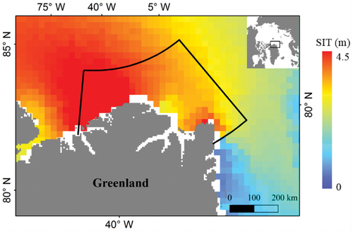
The polynya studied in this paper is situated in the north of Greenland, defined by 81–85° N, 5–50° W, as illustrated in Figure 1. This area is covered by thick sea ice, with a regional average thickness of 3.2 m recorded during the period 1979–2022. In recent years, several polynya events have occurred in this area, including the aforementioned the extreme 2018 winter polynya event, and pronounced summer polynyas events in 2018, 2020, and 2021.

Figure 1. The polynya studied in the paper, bounded by the black sector and northern coast Greenland, defined by 81–85° N, 5–50° W. The image is the average thickness of sea ice (denoted as SIT) from PIOMAS during the period 1979–2022.

3. Methods

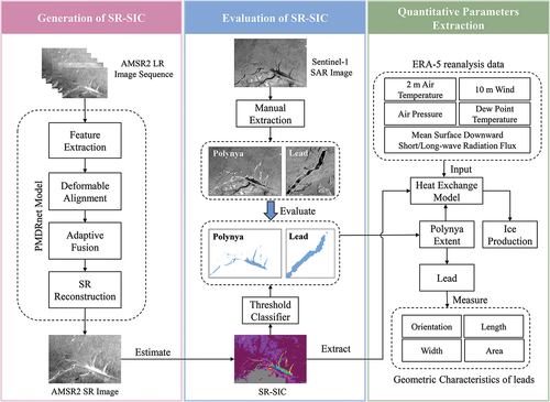
The method outlined in the paper is segmented into three main parts. This includes the generation of SR-SIC (in pink in Figure 2), the evaluation of SR-SIC by using its extracted polynya extent and geometric characteristics of leads (in blue in Figure 2), and the extraction of quantitative parameters of the polynya and leads from SR-SIC (in green in Figure 2).

Figure 2. Flowchart of the generation and evaluation of SR-SIC (in pink and blue, respectively), as well as the extraction of quantitative parameters of polynya and leads from SR-SIC (in green).

3.1. Generation of SR-SIC

As shown in Figure 2, a new state-of-the-art deep-learning-based MISR model, referred to as PMDRnet (Liu et al. 2022), is adopted to achieve finer SIC estimation by breaking through the limitation of the original coarse spatial resolution of AMSR2 images. It has been proven to have good capability to improve the spatial resolution of sea ice passive microwave data by a factor of four, which is beneficial for the reduction of mixed pixels at the ice–water divide and the uncertainties of SIC retrieval caused by coarse spatial resolution. In addition, PMDRnet exhibits superior SR performance compared to representative deep-learning-based MISR (DL-MISR) models (Liu et al. 2022). It is worth noting that PMDRnet utilized a novel progressive alignment strategy and multiscale deformable convolution alignment unit in the deformable alignment module, which can manage complex and large Arctic sea ice motions even with large geometric changes. Given the susceptibility of AMSR2 data at 89 GHz to atmospheric effects such as cloud liquid water and water vapor, PMDRnet incorporates an attention mechanism within the adaptive fusion module. This integration facilitates the adaptive fusion of effective spatiotemporal information across sequences. For high consistency of data distributions between the polynya region and the original training set of PMDRnet, including a large AMSR2 high-resolution and low-resolution (LR) image pair dataset for the entire Arctic region, PMDRnet’s optimal parameters are applied to the study area of this paper without retraining.

The ARTIST (Arctic Radiation and Turbulence Interaction Study) Sea Ice (ASI) algorithm (Spreen, Kaleschke, and Heygster 2008) is utilized to estimate SIC from SR AMSR2 images and uses the value of the polarization difference of the TB at 89 GHz channels. This can achieve excellent performance, similar to other SIC algorithms, without additional data sources as input but at higher spatial resolution. Furthermore, we utilize effective weather filters as suggested by Spreen et al. (2008) to eliminate spurious ice concentration resulting from atmospheric effects, such as cloud liquid water and water vapor. According to error estimation results provided by Spreen et al. (2008), errors especially at ice concentrations above 75% are less than 9%. Thus, SR-SIC is expected to achieve accurate extraction of polynyas and leads using an SIC threshold of 75%.

3.2. Evaluation of SR-SIC

To achieve the evaluation of SR-SIC for high-resolution monitoring of the polynya, we employ a manual approach to extract the polynya extent using SAR images serving as high-resolution products. Upon visual analysis of the high-resolution SAR images during the early opening period of the polynya, regions of polynyas and leads generally exhibit lower backscatter compared to the surrounding thicker ice, presenting darker signatures. This put together makes it possible to visually recognize the polynyas and leads in SAR images (Ivanova, Rampal, and Bouillon 2016), and obtain accurate polynya and lead extraction results with manual quality control. Finally, polynya extent can be obtained by summing the areas of all polynya pixels for each SAR image, and the geometric characteristics of leads in the polynya region can be measured.

In order to quantitatively describe the accuracy of the polynya extent and the width of leads extracted from SR-SIC, three commonly evaluation criteria are adopted, including precision, recall, and F1-Score (Kyzivat and Smith 2023). The precision (denoted as P) represents the probability of a true positive (denoted as TP) out of all the samples that are predicted to be positive, including TP and false positive (denoted as FP), calculated via equation (1). Recall (denoted as R) measures the probability of a TP out of the samples that are actually positive, consisting of TP and false negative (FN), shown in equation (2). F1-Score is used to find a balance between the performance of precision and recall, which is the inverse of the harmonic mean of the two (equation (3)). Taking polynya extent as an example, the precision is determined by dividing the number of correct AMSR2 polynya pixels belonging to the samples (judged as the polynya using both SAR and passive microwave data) by the number of all polynya pixels from only passive microwave data. The recall is determined by dividing the number of correct AMSR2 polynya pixels by all polynya pixels from only SAR images.

(1) $P=\frac{TP}{TP+FP}$(1)

(2) $R=\frac{TP}{TP+FN}$(2)

(3) $F1=\frac{2}{\frac{1}{P}+\frac{1}{R}}$(3)

3.3. Quantitative parameters extracted from SR-SIC

In order to quantitatively observe and characterize entire development process of polynyas, based on SR-SIC, some important parameters are extracted in this section, including polynya parameters at a larger scale such as polynya extent and ice production, as well as geometric parameters of leads around the polynya at a smaller scale, such as width and orientation. The extraction methods are described as follows.

3.3.1. Polynya extent and ice production

To derive the polynya extent from SR-SIC, a threshold of 75% is utilized (Cheng et al. 2017; Massom et al. 1998), and each pixel below the threshold is considered as a polynya pixel (i.e. open water and thin ice areas), where more pronounced heat exchange occurs and higher ice is produced than in non-polynya pixels (Gutjahr et al. 2016; Lei et al. 2020). Then, the polynya extent can be calculated by multiplying the accumulated polynya pixel number by the pixel area, equal to the square of the spatial resolution (1.5625 × 1.5625 km for AMSR2 SR images).

Ice production is estimated on a daily basis from SIC and heat flux is calculat by a method similar to that in previous studies (Cheng et al. 2017; Preußer et al. 2015), under the assumption that only the heat flux from the ice surface is considered while the oceanic heat flux from below is ignored. In addition, we assume that all the heat lost from the ice surface is used to produce ice, and that the heat exchange of the atmosphere–ocean interface occurs only in open water areas. The daily sea ice production volume $V$ is calculated by (4)

(4) $\mathrm{V}=tA\left(1-SIC\right)\frac{Q}{{\rho }_i{L}_f}$(4)

Where $t$ ( = 86,400 s) is the seconds of 1 day and ${\rho }_i$ (= 920 kg·m⁻³) is the sea ice density. $L_f$ (= 279 MJ·kg⁻¹) is the latent heat of sea ice fusion, expressed as the equation of sea ice temperature and sea ice salinity (Cheng et al. 2017). $Q$ (in W·m⁻²) is the net heat flux, which is estimated by the heat exchange model (Tamura, Ohshima, and Nihashi 2008), by using ERA-5 reanalysis data including 2 m air temperature, 10 m wind data, surface air pressure, 2 m dew point temperature, mean surface downward short-wave radiation flux, and mean surface downward long-wave radiation flux. $A$ (= 1.5625 × 1.5625 km for SR AMSR2 images) is the area of a pixel, and SIC is the sea ice concentration. Thus, the accuracy of SIC will have an important impact on the estimation of ice production associated with the heat fluxes and salt production in the upper ocean that impact global circulation, which can be achieved by improving the spatial resolution of AMSR2 images, with reduced mixed pixels at the ice–water divide and uncertainties in SIC estimation.

3.3.2. Geometric characteristics of leads

Based on the binary polynya map, some important geometrical characteristics of leads can be extracted, i.e. width and orientation, where the width of the lead has the impact on the heat exchange between the atmosphere and the ocean, as well as the orientation of the lead reflects the sea ice dynamics (Qu et al. 2021). Figure 3 presents the schematic diagram of geometrical characteristics of the lead, and the range here is consistent with that of Lead 1 region in Figure 4(c). First, the best-fitting line segment of the lead is acquired by minimizing the chi-squared error statistic for all the center points of lead pixels (Tschudi, Curry, and Maslanik 2002), shown as the green line in Figure 3. Then, the lead orientation is defined by measuring the angle clockwise between the best-fitting line and the average longitude, as shown in Figure 3. Taking quartile points of the best-fitting line segment as an example, the width of the lead at each quartile point is the minimum width in any direction in the image plane, i.e. the shortest distance between the two shores of sea ice passing through the quartile point, which is equal to the length of the red two-way arrow. Profiles where the widths of the lead at quartile points are located are indicated by the gray lines, denoted as P₁, P₂, and P₃. The mean width is calculated by dividing the area of the lead (filled in blue in Figure 3) in the region by the length of the best-fitting line segment (Qu et al. 2021). It is important to note that this length is not precisely equal to the length of a complete lead. Additionally, the length of a complete lead is not calculated considering that many leads extend beyond the coverage of the image.

Figure 3. Schematic diagram of geometrical characteristics of the lead (filled in blue), where the width and orientation of the lead are shown. The green line is the best-fitting line segment for lead pixels, and the grey lines show profiles where the widths of the lead at quartile points of the best-fitting line segment are located.

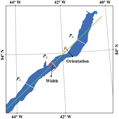
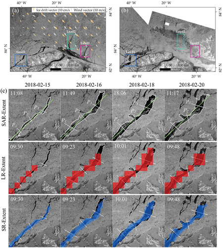
Figure 4. (a) the selected three major leads adjacent to the polynya, denoted as lead 1, lead 2, and lead 3, are enclosed by the blue box, the cyan box, and the magenta box, respectively. And the mean ice drift (yellow arrows) and the mean wind (light grey arrows) are shown from 15 to 22 February 2018. The background is sentinel-1 SAR image acquired on 16 February. (b) The sentinel-1 SAR image in the polynya area on February 23. (c) The results of lead 1 extracted from SAR-Extent (the white curve), LR-Extent (filled in red), and SR-Extent (filled in blue), which are covered to the corresponding sentinel-1 SAR images at four representative dates, including February 15, 16, 18, and 20. And the exact acquired time is marked in the upper left corner of each image.

4. Results

This section presents the results of observing the north Greenland polynya events using SR-SIC, including the 2018 winter polynya event and subsequent summer polynya events. When performing observations of the 2018 winter polynya event, the advantages of SR-SIC for the high-resolution monitoring of the polynya and leads are first illustrated separately. Then, the SR-SIC is used to observe the polynya and leads, including polynya observations at a larger scale (i.e. polynya extent and ice production) and lead characterization along the polynya at a smaller scale (i.e. lead width). On the other hand, three prominent summer polynya events in the north of Greenland starting in the winter of 2018 are also observed, and the ice condition is described using the different parameters of sea ice, such as SIC, sea ice thickness, and sea ice age, and the spatiotemporal distributions of which are present using the SR-SIC.

4.1. Results of the 2018 winter polynya event

4.1.1. Validation of SR-SIC

4.1.1.1. Polynya evaluation

To quantitatively evaluate the SR-SIC polynya observation results, we extract the polynya extents from SR-SIC (denoted as SR-Extent) using the threshold of 75% SIC outlined in Section 3.3.1. Additionally, we utilize the widely used SIC products provided by Bremen University, estimated from original AMSR2 images using the ASI algorithm (LR-SIC), and compare them with SR-SIC. The polynya extents from LR-SIC (denoted as LR-Extent) are also extracted using the same threshold. SR-Extent and LR-Extent are then compared with the polynya extent extracted from Sentinel-1 SAR images (denoted as SAR-Extent) to calculate the precision, recall, and F1-Score at three representative periods (14, 16, and 20 February 2018) before the polynya reaches the maximum extent, shown in Table 1. On the whole, the precision of SR-Extent (averaging 87.77%) is higher than that of LR-Extent (averaging 78.91%), meaning a lower error. The recall of SR-Extent (averaging 78.10%) is also higher than that of LR-Extent (averaging 71.68%), with more polynya pixels extracted. As for the F1-Score, SR-Extent has better evaluation results than LR-Extent at these three dates, in particular, for the polynya on 14 February, belonging to the early stage of polynya formation with a smaller size and narrower shape (Figure 5(g)). It is more challenging to identify accurately this polynya via the LR-SIC map (Figure 5(a)); however, the precision using SR-SIC is 12.80% higher than that using LR-SIC and the recall and F1-Score are 9.37% and 10.83% higher respectively. This shows that the SR-SIC map with a higher spatial resolution provides more accurate extraction of polynya extent and finer observation of entire polynya development process.

Figure 5. Results of LR-Extent (filled in red) and SR-Extent (filled in blue), compared with SAR-Extent (the white line) at three representative periods (14, 16, and 20 February 2018) before polynya reaches the maximum extent. And some leads which can be identified by SR-Extent but not by LR-Extent are marked by the red arrows.

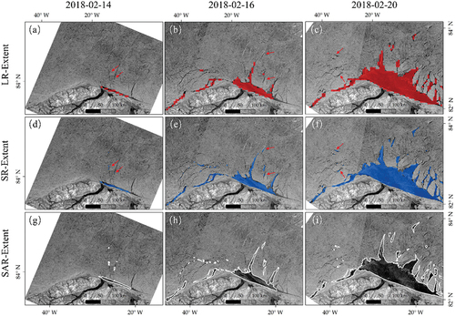
Table 1. Precision, recall, and F1-score of LR-Extent and SR-Extent, compared with SAR-Extent at three representative periods (14, 16, and 20 February 2018) before the polynya reaches the maximum extent. And the improvements of SR-Extent results compared to LR-Extent results are also given.

Date	Polynya extent	Precision (%)	Recall (%)	F1-Score (%)
14 February	LR-Extent	69.34	53.65	60.49
	SR-Extent	82.14	63.02	71.32
	Improvement	12.80	9.37	10.83
16 February	LR-Extent	79.28	72.04	75.49
	SR-Extent	87.14	79.54	83.17
	Improvement	7.86	7.50	7.68
20 February	LR-Extent	88.10	89.36	88.73
	SR-Extent	94.03	91.74	92.88
	Improvement	5.93	2.38	4.15

In addition, the results of the LR-Extent (filled in red in Figure 5) and the SR-Extent (filled in blue in Figure 5) on 14, 16, and 20 February are covered in the corresponding Sentinel-1 SAR images for visual comparisons, and SAR-Extent (white line) serves as the reference, as shown in Figure 5. Overall, SR-Extent has better consistency with the SAR-Extent than the LR-Extent. Additionally, SR-Extent is better at locating the edges of the polynya and leads because its higher spatial resolution allows for sharper gradients. Furthermore, much smaller leads can be identified by SR-Extent than by LR-Extent, such as leads above the polynya on 14 February, on the upper right side of the polynya on 16 February and on the upper left side of the polynya on 20 February, marked by the red arrows in Figures 5(a-f).

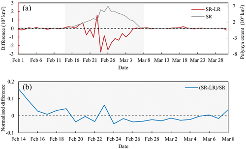
On the other hand, the open water extent (OWE) in the polynya region is also calculated to further illustrate the benefits of the high-resolution SR-SIC by using a 15% SIC threshold, that is, each pixel in this area has at least 85% open water, as shown in the Figure 6. There are 16 open water fractions in the SR-SIC map for each AMSR2 LR-SIC grid cell, since the upsampling scale of image SR is 4. It is worth mention that when the mean open water fraction of both SR-SIC and LR-SIC are below 85% for the same LR-SIC grid cell, some open water fractions in SR-SIC may be above 85%, and vice versa, thanks to the benefits of higher spatial resolution leading to sharper gradients. But the open water fractions of the most LR-SIC grid cells in the polynya region are below 85%, especially during the early opening period of the polynya. That is because that the polynya during this period has a narrow opening and many mixed pixels, resulting in the challenge of detecting areas with the open water fraction exceed 85% for LR-SIC. Thus, SR-SIC, with higher spatial resolution, is expected to have larger OWE than LR-SIC with its lower spatial resolution (Ludwig et al. 2019). The result shows that the overall difference (red line in Figure 6(a)) in the OWE from SR-SIC and from LR-SIC is relatively small compared to the absolute value of the OWE from SR-SIC (gray line in Figure 6(a)). However, the OWE from SR-SIC is greater than that from LR-SIC for the whole time series, with a significantly larger difference during the opening period of the polynya lasting from February 14 to March 8 (Figure 6(b) and shaded time periods in Figure 6(a)). Additionally, the normalized differences are also all above zero, and are larger during the early opening (February 14 to 17) and freezing period (February 28 to March 3) and smaller when the polynya is fully opening (around February 26) (Figure 6(b)), excluding February 23 due to the smaller absolute value of OWE. At the times represented by the points marked with red pentagrams in Figure 6(b) correspond to the LR-SIC and SR-SIC shown in Figure 7. Their distributions are illustrated in Figure 8, providing a more intuitive comparison between OWE from LR-SIC and SR-SIC. On 14 February, the normalized difference is close to 1 due to the OWE value from LR-SIC of 0, resulting from the coarse spatial resolution of LR-SIC, whose visualization comparison can be seen in Figures 7(a,m) and Figure 8(a).

Figure 6. (a) time series of difference in OWT oriented from LR-SIC and SR-SIC (red line), and the absolute value of the OWE from SR-SIC (grey line). And (b) shows the normalized difference from 14 February to 8 March marked by the grey shading in (a), belonging to the opening period of the polynya. Red pentagrams show that these times have corresponding SIC maps in Figure 7, whose detailed descriptions are also labeled next to them.

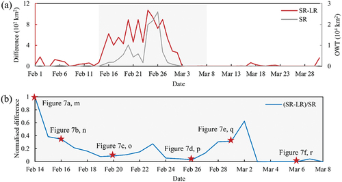
Figure 7. LR-SIC and SR-SIC at the representative periods of the polynya from opening to closing, where the corresponding polynya extent extracted from AMSR2 SIC using the threshold 75%, denoted as LR-Extent (filled in red) and SR-Extent (filled in blue). The AMSR2 images are acquired on 14, 16, 20, 26 February and on 1, 6 March, respectively. There are some narrow leads in the areas enclosed by boxes and some floating ices in the areas enclosed by circles.

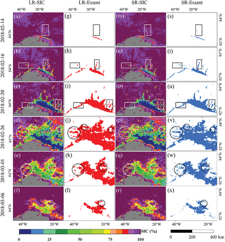
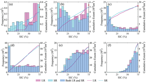
Figure 8. The SIC distribution and cumulative extent of the LR-SIC and the SR-SIC at different development stages of the polynya. The red symbol “×” in (a), (b), and (c) indicate the polynya extent extracted from SAR images in Figure 5.

Therefore, integrating the evaluation results of SR-SIC at the polynya scale from the two aforementioned perspectives demonstrates that SR-SIC exhibits a superior capability (such as an average 7.55% improvement in F1-Score for the polynya extent and the enhanced detection capabilities for open water areas within the polynya area) of monitoring polynyas compared to LR-SIC.

4.1.1.2. Lead evaluation

In addition to the dynamic monitoring of the 2018 winter polynya, we evaluate the feasibility of using the results of SR-Extent in the study region to observe and characterize finer leads.

There are three representative leads adjacent to the polynya, as shown in the boxes of Figure 4(a). These begin to develop gradually as the polynya area increases on February 15, and finally become a part of the polynya or floating ice region and no longer appear in a narrow shape on around February 23. This is due to the rapid expansion of the polynya, as shown in the Sentinel-1 SAR image in the polynya area on February 23 in Figure 4(b). The narrowest lead, Lead 1, is taken for lead evaluation. Its boundaries from LR-Extent and SR-Extent are compared with those of SAR-Extent at four representative dates via considering its development and the availability of high-quality Sentinel-1 SAR images, as shown in Figure 4(c). Compared with the dates chosen for the evaluation of SR-SIC in polynya extent, February 14 is not chosen due to the nonoccurrence of Lead 1, and February 15 and 18 are added because high-quality SAR images are available for the area.

The results show that the boundary of Lead 1 from SR-Extent at each date (the third line from the top in Figure 4(c)) is more consistent with that of SAR-Extent because of its high spatial resolution with more detailed gradient information and reduced uncertainty compared with that from LR-Extent (the second line from the top in Figure 4(c)). The shape of Lead 1 in LR-Extent is very coarse and its opening is usually much larger than that of SAR-Extent. In addition, it is more difficult to resolve the relatively narrow part of Lead 1 when using LR-Extent, especially at the early stage, such as on February 15. Therefore, the finer SR-Extent can obtain more accurate geometric characteristics of leads, including width, orientation, and length, which can be utilized to further investigate the differences in their development processes and analyze their potential causes by combining meteorological data, such as 2 m air temperature and 10 m wind data, as well as sea ice drift products.

Table 2 shows the results for the mean widths and the widths at the three different profiles of Lead 1 from LR-Extent, SR-Extent and SAR-Extent on February 15, 16, 18, and 20 in Figure 4(c), where the mean width is related to the lead area, length and orientation of the lead. The location of each profile (marked by the gray line in Figure 4(c)) is determined by the width of Lead 1 passing each quartile point of the best-fitting line segment of Lead 1 (the green line in Figure 4(c)) in SAR-Extent, denoted as P₁, P₂, and P₃ from left to right in each image. The profiles of Lead 1 in LR-Extent and SR-Extent are the same as that in SAR-Extent, that is, the position of the corresponding gray line in each image is the same in each column of Figure 4(c). For the mean width of Lead 1 at each time period, the results from SR-Extent are closer to those from SAR-Extent on the whole, whose bias is less than 0.5 km on February 16, 18, and 20, and a little larger on February 15 with a value of 1.13 km. Meanwhile, the mean width from LR-Extent is much larger than that from SAR-Extent, with bias ranging from 1.75 km to 2.90 km.

Table 2. Mean widths and widths at the three different profiles of lead 1 extracted from LR-Extent, SR-Extent and SAR- Extent, whose acquisition dates are on February 15, 16, 18, and 20.

			Width at profiles
			P1			P2			P3
Date		Mean width (km)	Width (km)	Precision /recall (%)	F1-Score (%)	Width (km)	Precision /recall (%)	F1-Score (%)	Width (km)	Precision /recall (%)	F1-Score (%)
Feb 15	LR	4.42	3.23	41.27/ 63.33	49.97	4.22	39.81/ 100.00	56.95	0	0	/
	SR	3.09	3.23	41.27/ 63.33	49.97	2.9	57.93/ 100.00	73.36	2.53	76.28/ 97.47	85.59
	SAR	1.96	2.10	/	/	1.68	/	/	1.98	/	/
Feb 16	LR	7.32	10.54	49.24/ 100.00	65.99	0.50	100.00/ 12.32	21.93	7.10	69.44/ 100.00	81.96
	SR	4.77	6.19	83.84/ 100.00	91.21	4.94	82.19/ 100.00	90.22	5.31	92.84/ 100.00	96.29
	SAR	4.45	5.19	/	/	4.06	/	/	4.93	/	/
Feb 18	LR	8.62	8.83	49.72/ 61.14	54.84	3.62	89.78/ 69.89	78.60	13.31	58.83/ 100.00	74.08
	SR	5.51	6.60	96.82/ 89.00	92.74	4.89	94.27/ 99.14	96.65	7.83	100.00/ 100.00	100.00
	SAR	5.72	7.18	/	/	4.65	/	/	7.83	/	/
Feb 20	LR	7.96	9.70	78.45/ 100.00	87.93	0.63	100.00/ 14.62	25.51	13.11	58.58/ 85.62	69.57
	SR	5.77	7.16	92.74/ 87.25	89.91	3.25	100.00/ 75.41	85.98	8.21	93.54/ 85.62	89.41
	SAR	6.21	7.61	/	/	4.31	/	/	8.97	/	/

Similarly, compared with the widths of SAR-Extent at three profiles, those measured based on LR-Extent are wider, with the absolute difference of a minimum of 1.03 km and maximum 5.36 km, except for P₂ on February 18, which is slightly smaller. Additionally, the widths of LR-Extent at P₃ on February 15, P₂ on February 16, and P₂ on February 20 are equal to or close to zero with a very low recall, while the widths based on SR-Extent are close to those of SAR-Extent and have a much higher recall, indicating that LR-Extent’s lead identification ability is worse due to low spatial resolution. Overall, the F1-Score of SR-Extent is much higher than those of LR-Extent, illustrating that the location and geometrical shape of the leads obtained from SR-Extent is more similar to that of SAR-Extent.

4.1.2. High-resolution monitoring using SR-SIC

4.1.2.1. Polynya observations

As shown in Figure 7, six representative periods of the polynya from opening to closing are chosen for observation of the development of the 2018 winter polynya both temporally and spatially via AMSR2 SIC (i.e. LR-SIC and SR-SIC) and polynya extent extracted from AMSR2 SIC using the threshold of 75% SIC (i.e. LR-Extent and SR-Extent). Based on the SR-SIC and SR-Extent maps, in the early stage, the polynya takes the form of a long and narrow lead along the north of Greenland, as shown in Figures 7(m,s). The polynya starts to open and is already visible in the maps on 16 February (Figures 7(n,t)), then steadily breaks up parallel to the coast to increases into a larger opening on 20 February (Figures 7(o,u)), and reaches its maximum extent on 26 February with an extent of more than 70,000 km² (Figure 9(a)). Afterwards, the polynya begins to freeze and close on 1 March (Figures 7(q,w)), with increasing newly formed and thickened ice. It is no longer identified as open water in the SR-SIC map but appears as an ice–water mixing region with gradually increasing SIC. On 6 March, the polynya is nearly closed and most of the polynya region are retrieved as fully sea ice covered (Figures 7(r,x)).

Figure 9. (a) time series of differences in the polynya extent oriented from LR-SIC and SR-SIC (red line), and the absolute value of the polynya extent from SR-SIC (grey line). And (b) shows the normalized difference from 14 February to 8 March marked by the grey shading, belonging to the opening period of polynya.

In Figure 8, we present statistical histograms of SIC distribution of LR-SIC and SR-SIC in the polynya region where the SIC value is less than 75%, complementing the information presented in Figure 7. Thanks to the higher spatial resolution of the SR-SIC map, we can obtain a more detailed spatial distribution of polynya, including the position of polynya edge as well as distribution characteristics of sea ice inside the polynya, when compared to the LR-SIC map. For example, on 14 February, the SR-SIC map (Figure 7(m)) can resolve the finer shape and structure of the polynya with a small opening, unlike the LR-SIC map (Figure 7(a)) due to its coarse spatial resolution. In addition, some SIC values inside the polynya on 14 February are about 40% in the LR-SIC map (Figures 7(g), 8(a)), which are recognized as open water pixels because their SIC values are less than 15% in the SR-SIC map (Figures 7(s), 8(a)). This is due to the higher spatial resolution of SR-SIC, resulting in fewer mixed pixels and sharper gradient information. In addition, compared with the LR-SIC map, the SR-SIC map shows more relatively narrow leads connected to the polynya, such as leads enclosed by the boxes in Figures 7(s,t,u). The floating ice found in the polynya region (enclosed by circles) also have much sharper sea ice edges and finer texture in the SR-SIC map (Figures 7(p,q,r)). Therefore, the SR-SIC, with its improved spatial resolution, is useful to achieve finer dynamic monitoring of leads and floating ice, contributing to a more detailed description of polynya development.

Afterward, the polynya extent is extracted from SR-SIC and LR-SIC separately for February and March 2018, and the comparison of LR-Extent and SR-Extent is shown in Figure 9. The absolute value of SR-Extent is shown in Figure 9(a) (gray line), which shows that the polynya extent begins to increase on 14 February until reaching a maximum of more than 70,000 km² on 26 February, then gradually declining toward zero around March 8. Moreover, it can be seen that the difference between LR-Extent and SR-Extent is relatively large during the opening period (marked by the shaded gray box) of the polynya from their difference plot in Figure 9(a) (red line). Here, SR-Extent is smaller than LR-Extent, mainly over February 20–22 and February 24–March 5, and larger during the remaining dates of the opening period. It is possible that, compared with LR-SCI, the single pixels of SR-SIC with improved spatial resolution has higher homogeneity, leading to a clearer ice – water boundary and difference in the polynya extent. When the LR-SIC shows larger extent than SR-SIC, such as on February 20 (Figure 7(o)), there are many pixels in polynya boundary area that show SIC values of slightly less than 75% in the former (Figures 7(c), 8(c)). This are considered polynya pixels in LR-SIC, but they are resolved as non-polynya pixels in the SR-SIC image. In addition, as depicted in Figures 8(a-c), the polynya extent of SR-SIC in the polynya region on February 14, 16, and 20, 2018, is closer to those extracted from SAR images in Figure 5 compared to those of LR-SIC. Compared to the normalized difference during the opening period (Figure 9(b)), the normalized difference during the lead period is large, reaching nearly 0.2 on February 14, then fluctuating in the range [−0.05, 0.05] in the following days.

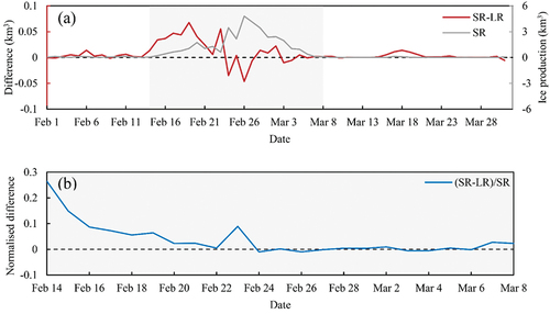
The ice production of the polynya identified in the SR-SIC during February and March 2018 are shown in Figure 10(a) (gray line), with a trend consistent with polynya extent, and the difference compared to LR-SIC is shown by the red line. The figure shows lower ice production in SR-SIC, mainly over February 24–27 and March 3–5, compared with that of LR-SIC. Their normalized difference reaches up to 0.36 on February 14, declining steadily to almost zero on February 24 because of a small difference between the ice production in LR-SIC and SR-SIC.

Figure 10. (a) time series of differences in the ice production oriented from LR-SIC and SR-SIC (red line), and the absolute value of the ice production from SR-SIC (grey line). And (b) shows the normalized difference from 14 February to 8 March marked by the grey shading in (a), belonging to the opening period of polynya.

4.1.2.2. Leads characterisation

After achieving polynya observations at a large scale using SR-Extent, the next focus will be on lead characterization at a smaller scale by exploring the development of three leads next to the polynya (Figure 4(a)). These three leads are located in different locations within the polynya. Lead 1 is positioned furthest from the polynya, near the north-west coast of Greenland. Lead 2 is directly north of the polynya, and Lead 3 is located to the northeast of the polynya.

Initially, we conduct the best fit for the lead pixels of Lead 1, 2, and 3 extracted from SR-Extent, completing measurements of orientation and length and performing area calculations, with the specific values detailed in Table 3. The results indicate that from February 15 to 22, Lead 1 exhibits minimal changes in orientation, with differences within 3°. Conversely, based on the measurements of orientation, Lead 2 consistently demonstrates a trend of moving away from the edge of the polynya, with the absolute values of its area and length surpassing those of Lead 1 during the same period. For Lead 3, its orientation gradually shifted closer to the edge of the polynya from February 15, with both area and length progressively increasing. Additionally, to indicate the speed of their development, we further calculate the time series of the mean width of these three leads, as illustrated in Table 3 and Figure 11(a), as it is associated with its area, length and orientation of the lead. Lead 3 has the smallest mean width of 1.02 km at the beginning, but it increases rapidly from February 18 and surpasses the other two, reaching a maximum width of 27.38 km on February 21, 2.25 times that of Lead 2 and 3.85 times that of Lead 1. Compared to Lead 3, the mean width of Lead 2 widens slowly, reaching a maximum of 12.39 km also on February 21, while the mean width of Lead 1 changes more slowly, mostly around 5 km, with a maximum of 6.59 km, also on February 21 and a minimum of 2.84 km on February 15.

Figure 11. (a) the mean widths, (b) 10 m wind speed and (c) 2 m air temperature for lead 1, lead 2, and lead 3, and (d) ice drift speed for lead 2 and lead 3 during the period February 15 to 22, 2018.

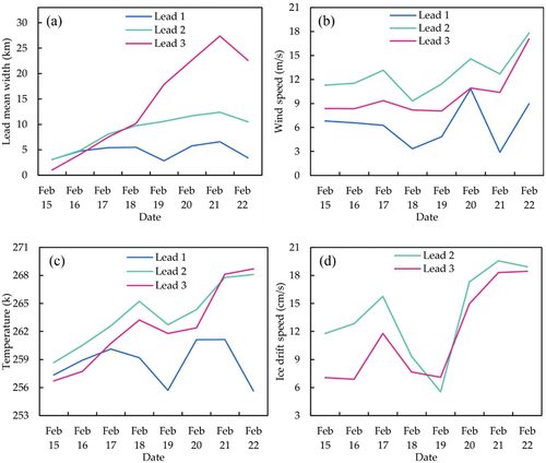
Table 3. Measurements for orientation, area, and length of leads 1, 2, and 3 utilizing SR-Extent during the period from February 15 to 22, 2018.

Date		Feb 15	Feb 16	Feb 17	Feb 18	Feb 19	Feb 20	Feb 21	Feb 22
Lead 1	Orientation (°)	50.38	49.27	47.47	48.23	48.59	49.59	48.79	48.18
	Area (km^2)	195.31	336.50	361.67	363.73	183.08	366.36	476.57	139.18
	Length (km)	68.77	70.51	66.56	65.98	64.39	63.53	72.37	40.77
	Mean width (km)	2.84	4.77	5.43	5.51	2.84	5.77	6.59	3.41
Lead 2	Orientation (°)	23.92	21.54	13.67	16.18	11.56	4.33	356.35	352.38
	Area (km^2)	229.98	469.42	607.24	797.43	776.74	777.70	774.69	544.88
	Length (km)	75.04	96.00	75.29	81.86	73.44	66.45	62.52	51.80
	Mean width (km)	3.06	4.89	8.07	9.74	10.58	11.70	12.39	10.52
Lead 3	Orientation (°)	22.18	29.39	30.83	37.51	48.94	64.79	79.50	64.22
	Area (km^2)	29.33	215.09	449.16	705.3	1201.8	1374.12	1633.94	1499.89
	Length (km)	28.74	52.26	59.94	69.29	67.36	60.71	59.67	66.34
	Mean width (km)	1.02	4.12	7.49	10.18	17.84	22.63	27.38	22.61

4.2. Results of summer polynya events

4.2.1. Sea ice conditions

Some remarkable summer polynya events have occurred since this unprecedented winter event (Lei et al. 2020; Schweiger et al. 2021; Shen et al. 2021). Note that a polynya event typically occurs in the ice-freezing season, but this region is generally covered by thick, old sea ice, even in summer, with a higher SIC. Based on the NSIDC SIC daily product, the mean SIC for the entire year over 1979–2017 in the study region is around 98%, and even about 95% in summer (July to September). Thus, when the SIC of this region is relatively low during summer it is also considered a polynya event. Compared to the climatological normal of 1979 to 2017, there are several occurrences of lower mean SIC in August of the years between 2018 and 2022, especially 2018, 2020, and 2021, where their SIC deviates by more than 1 standard deviation from the climatological normal, as illustrated in Figure 12(a). In particular, the polynya region in 2020 experiences an August record-low 42% SIC minimum during the 44-year period (1979–2022) (Figure 12(b)), even lower than the significantly low SIC minimum of earlier years, such as 48% in 1985 and 59% in 1991 (given the scope of this paper, only 2018 and subsequent years are discussed.) As the Figure 12(a) shows, the 2018 summer polynya lasts from 15 July to 5 September, the 2020 summer polynya from 26 July to 6 September, and the 2021 summer polynya from 6 August to 15 September. Here, the regional mean SIC value of 95% is used as a cutoff to determine the time range of the polynya event. Thus, the period from 15 July to 15 September is investigated in this section, covered by the black box in Figure 12(a).

Figure 12. (a) regional mean SIC in the study region for 2018 (red line), 2019 (cyan line), 2020 (green line), 2021 (blue line) and 2022 (orange line). The grey line shows the 1979–2017 climatological normal, and the grey shading indicates within 1 standard deviation. The focused time from 15 July to 15 September is covered by the black box. (b) Time series of minimal SIC for August. The SIC data in (a) and (b) are from the NSIDC SIC product. (c) Mean ice thickness and (d) mean ice age in the study region for 2018 (red line), 2020 (green line), and 2021 (blue line). The grey line shows the corresponding climatological normal (during 1979–2017 for (c) and during 1984–2017 for (d)), and the grey shading indicates within 1 standard deviation.

In addition, the mean thicknesses of the summer in 2018, 2020, and 2021 are also significantly lower than the standard deviation of the 1979–2017 climatology (Figure 12(c)). However, from April to June of 2020 the mean ice thickness is unusual: 2.75 m thicker on average than in the summer of 2020. Moreover, the mean sea ice age for 2018, 2020, and 2021 is generally below the standard deviation of the 1984–2017 climatology, indicating that the sea ice in this region is becoming younger, as Figure 12(d) shows. The mean ice age of the 2020 summer polynya period reaches its lowest point in mid-August, when the mean SIC also reaches its lowest level on record. However, an anomaly in mean sea ice age also occurs in 2020 from January to July, with more old sea ice than in 2018 and 2021. However, it seems that this thick and old sea ice is insufficient to prevent the summer SIC in 2020 from reaching a record-low minimum.

4.2.2. Spatiotemporal distribution

Figure 13(a) shows the time series of the polynya extent from SR-SIC with improved spatial resolution during the period from 15 July to 15 September for 2018, 2020, and 2021. Overall, the polynya extent maximum and mean are higher in 2020 than in 2021 and smallest in 2018, and the summer polynyas in 2020 and 2021 are larger in size than that of 2018 as well as compared to the winter polynya. The rapid increase in the polynya extent occurs the earliest in 2020, followed by 2018, and the latest in 2021, while the rapid decrease occurs the earliest in 2018, followed by 2021, and the latest in 2020. However, in early September of 2021 there is still a greater polynya extent compared with the same time in 2018 and 2020. Moreover, the polynya extent in 2020 oscillates in August, reaching a maximum of 95,000 km² and a minimum of around 20,000 km².

Figure 13. (a) time series of the polynya extent oriented from SR-SIC during the period from 15 July to 15 September for 2018 (red line), 2020 (green line), and 2021 (blue line). The spatial frequency maps of polynya occurrence during the period from 15 July to 15 September for (b) 2018, (c) 2020, and (d) 2021.

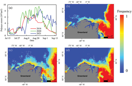
The spatial frequency maps of polynya occurrence during the period from 15 July to 15 September for 2018, 2020, and 2021 are presented in Figures 13(b,c,d) respectively. The comparison shows that the largest spatial distribution of polynya occurrence is in 2020 and the smallest in 2018. In addition, for all 3 years, it can be clearly observed that polynya gradually occurs less frequently from near the shore to further away along the northern part of Greenland, which is very similar to the development process of the winter polynya in 2018. This may be related to the formation mechanism of the polynya in this region, such as that of anomalous offshore winds: sea ice close to the northern part of Greenland is blown away earlier to form early polynya in the form of leads. This contributes to areas remaining as open water or thin ice regions for a longer period, increasing the frequency of polynya occurrence.

5. Discussion

In this section, we discuss the potential causes of the differences in the development of leads along the 2018 winter polynya in the north of Greenland. Additionally, the possible reasons for the occurrence of summer polynya events of 2018, 2020, and 2021 are investigated.

5.1. Potential causes related to lead development

To analyze the causes of the different development processes of the above three leads occurring along the 2018 winter polynya, we consider 10 m wind speed, 2 m air temperature, and sea ice drift data, as shown in Figures 11(b-d). This is undertaken as existing studies suggest that this polynya is caused by unusual southerly winds, where the sea ice drifts northwards instead of southwards as usual, and the trigger of the event is a sudden stratospheric warming (Moore et al. 2018).

The change in both wind speed and temperature in the Lead 1 area are slow when compared to the Lead 2 and Lead 3 areas, except for the temperature data on February 15 and 16, where the Lead 1 values are slightly higher than that in the Lead 3 area. The wind speeds in Lead 2 and Lead 3 areas start slowly increasing until February 21 when it increases rapidly, and the respective temperatures increase much faster. Additionally, the wind speed and temperature in the Lead 2 area are always higher than those in the Lead 3 area, except for temperature on February 21 and 22. There is a lack of sea ice drift data for the Lead 1 area due to its proximity to the coast of Greenland, but it seems that the sea ice drift speed in this area is much lower than those of the Lead 2 and Lead 3 areas, as the spatial distribution of the mean sea ice drift in Figure 4(a) shows. The trends of sea ice drift speed in the Lead 2 and Lead 3 areas are basically the same: they starting showing an increasing trend, decreasing rapidly on February 17, reaching a minimum on February 19 and then increasing rapidly. However the overall sea ice drift speed in the Lead 2 area is higher, which is consistent with the spatial distribution of the mean drift speed in Figure 4(a), with the angle between the mean drift speed direction and the mean orientation close to 45° for Lead 2 and 90° for Lead 3. Additionally, the mean temperature is also lower in the Lead 1 area compared to that in the Lead 2 and Lead 3 areas; the higher temperature slows down the formation and freezing of sea ice on the surface of the leads, thus contributing to their development. Similarly, the mean wind speed is the lower in Lead 1 compared to that in Lead 2 and Lead 3, while the angles between the mean wind direction and the mean orientation are close to 45° to the three leads. Additionally, the angle between the wind direction and the ice drift speed direction as well as the mean orientation of leads is often one of the most important factors in the widening and lengthening of leads when either the wind speed or ice drift speed is relatively high.

Therefore, it is expected that the lead development is related to wind speed, temperature, and ice drift. This is based on Lead 1 developing more slowly with slower wind speed and ice drift speed as well as lower temperature, while Lead 2 and Lead 3 show the inverse. However, it cannot explain why Lead 3, with a slower speed and lower temperature, develops faster than Lead 2. In addition to factors such as ice thickness and ice structure, it may be related to the angle between the drift direction of sea ice and the orientation of the lead, with Lead 3 approaching 90°, and tending to be wider, while the Lead 2 approaching 45°, and tending to be longer.

5.2. Environment factors related to Summer polynya events

The cause of polynya formation is usually associated with the melting of sea ice due to high temperatures or sea ice drift driven by strong winds, known as sensible heat and latent heat polynya, respectively (Lei et al. 2020). Therefore, we carry out a comprehensive analysis of air temperature, regional wind, and sea ice motion so as to investigate the contributions of possible environmental factors on the formation and development of these three summer polynyas, as well as different spatiotemporal distribution characteristics.

As Figure 14(a) shows, for each summer polynya event, the air temperature increases rapidly at the early stage of the polynya event, such as the periods of 21 July to 3 August in 2020, 26 July to 3 August in 2021, and July 29 to August 5 in 2018. On these dates, the air temperature significantly exceeds the 1979–2017 climatological normal and is above freezing, with a maximum of 2 to 4°C. The temperature firstly falls back to the freezing point on 11 August in 2021 and on 14 August in 2018 and in 2020, when the polynya extents (Figure 14(d)) are greater. This may be related to the formation and thickening of newly ice in the polynya region. However, on the whole, the duration of air temperatures above the freezing point is short and its absolute value is relatively low, which may delay ice freezing, allowing the opening of polynya to continue. However, the main cause of polynya formation demands further exploration.

Figure 14. (a) mean 2 m air temperature, (b) mean 10 m wind, (c) mean sea ice motion, and (d) mean polynya extent in the study region during the period from 15 July to 15 September for 2018 (red line), 2020 (green line), and 2021 (blue line). The grey line shows the 1979–2017 climatological normal. (e) Time series of sea ice thickness (black line) and the correlation coefficient (red line) of summer between wind and sea ice motion from 1979 to 2021.

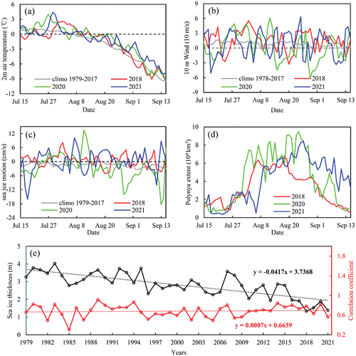
When examining the time series of regional wind in Figure 14(b), it is found that the wind speed oscillates above and below the 1979–2017 climatological normal during all three summer polynya events, with a maximum of 6.36 m/s and a minimum of −6.11 m/s (positive implying offshore wind and negative implying onshore wind). Compared to the wind speed of the winter polynya event in 2018, with a maximum of 13.20 m/s, the absolute magnitude of the wind speed of the three summer polynya events is moderate. Additionally, the wind during the opening period of the summer polynya events is mostly offshore wind, which is the same direction as the 1979–2017 climatological normal. Although the unusual southerly wind is the cause of the 2018 winter polynya event, there may be other determining factors causing the formation and development of the above summer polynya events given that the regional wind shows a moderate speed.

On the other hand, when comparing the time series of wind and sea ice motion, it is found that the pattern of sea ice motion appears to be highly correlated with wind speed, with the same changing trend. In addition, both the sea ice motion speed and direction during the opening period of the summer polynya events are anomalous (Figure 14(c)), especially in 2020 when the sea ice drifts offshore at speeds of up to 13.49 cm/s. In addition, following Shen et al. (2021) illustrates that thinner ice responds more to wind and is more prone to drift, favoring polynya opening. Thus, sea ice thickness and the relationship between wind and sea ice motion in the study area is discussed and whose time series is presented in Figure 14(e). It is true that sea ice in the north of Greenland during summer also becomes thinner (black line in Figure 14(e)), in line with current sea ice conditions throughout the Arctic region following a general thinning trend. In addition, the calculated correlation coefficient between wind and sea ice motion from 1979 to 2021 (red line in Figure 14(e)) shows an increasing trend when sea ice gradually thins. Compared to 2018 and 2021, the sea ice in 2020 is thicker, but the correlation coefficient between wind and sea ice motion reaches 0.82 in 2020, 0.78 in 2018, and 0.56 in 2021. This is because the absolute value of sea ice thickness in 2020 is still very thin over the whole time series, and the spatial distribution of thick ice in the polynya region also has an impact. Additionally, the wind speed in 2020 is also faster than in 2018 and 2021, and this causes a larger offshore drift of thinning sea ice when affected by offshore wind, which follows the occurrence of polynyas. This could also explain the fact that the summer SIC in 2020 reaches the lowest on record, when the polynya is also the largest in size and longest lasting.

6. Conclusions

In this paper, a state-of-the-art DL-MISR algorithm, PMDRnet, is utilized to obtain SR-SIC with a fourfold improvement in spatial resolution, allowing for finer observation and accurate characterization of north Greenland polynyas. The evaluation results demonstrate that SR-SIC exhibits superior monitoring capabilities for sea ice at both the polynya and lead scale compared to the original LR SIC, with an average 7.55% improvement of F1-Score for polynya extent and 31.17% for lead width. Using the SR-SIC, with lower uncertainties and reduced mixed pixels compared to LR-SIC, more SIC values below 40% are distinguished, enhancing detection capabilities for open water areas within the polynya. In addition, the leads with narrow openings less than 3 km along the 2018 winter polynya can be well detected utilizing SR-SIC. This allows us to obtain the detailed spatial distribution of ice/water in the polynya region. Therefore, the entire evolution process of polynyas, including polynya extent and ice production, can be characterized more accurately. Finally, it is concluded that the lead development along the 2018 winter polynya is related to wind, air temperature, and ice drift. Additionally, we found that the thinner sea ice in the polynya region in the summer might contribute to the formation and development of the summer polynya events of 2018, 2020, and 2021 under moderate regional wind speed.

Acknowledgments

The authors would like to acknowledge JAXA (https://global.jaxa.jp/) for providing the AMSR2 brightness temperatures; European Space Agency for providing Sentinel-1 SAR images; NSIDC for providing the sea ice products including SIC, ice motion, and sea ice age; the Polar Science Center at the University of Washington for providing the sea ice thickness products; ECMWF for providing the ERA-5 reanalysis data.

Disclosure statement

No potential conflict of interest was reported by the author(s).

Data availability statement

The super-resolved passive microwave sea ice concentration for the polynya region in northern Greenland is available at https://github.com/TJxiaominliu/Super-Resolved-Passive-Microwave-Sea-Ice-Concentration. The dataset presented in this study is available on request from the corresponding author.

Additional information

Funding

This work was supported by the National Key Research and Development Program of China [2021YFB3900105]; the National Science Foundation of China [42371362].

References

- Beitsch, A., L. Kaleschke, and S. Kern. 2014. “Investigating High-Resolution AMSR2 Sea Ice Concentrations During the February 2013 Fracture Event in the Beaufort Sea.” Remote Sensing 6 (5): 3841–24. https://doi.org/10.3390/rs6053841.
- Brown, L. C., S. E. L. Howell, J. Mortin, and C. Derksen. 2014. “Evaluation of the Interactive Multisensor Snow and Ice Mapping System (IMS) for Monitoring Sea Ice Phenology.” Remote Sensing of Environment 147:65–78. https://doi.org/10.1016/j.rse.2014.02.012.
- Casey, J. A., S. E. L. Howell, A. Tivy, and C. Haas. 2016. “Separability of Sea Ice Types from Wide Swath C- and L-Band Synthetic Aperture Radar Imagery Acquired During the Melt Season.” Remote Sensing of Environment 174:314–328. https://doi.org/10.1016/j.rse.2015.12.021.
- Cheng, Z., X. Pang, X. Zhao, and C. Tan. 2017. “Spatio-Temporal Variability and Model Parameter Sensitivity Analysis of Ice Production in Ross Ice Shelf Polynya from 2003 to 2015.” Remote Sensing 9 (9): 934. https://doi.org/10.3390/rs9090934.
- de Gelis, I., A. Colin, and N. Longepe. 2021. “Prediction of Categorized Sea Ice Concentration from Sentinel-1 SAR Images Based on a Fully Convolutional Network.” IEEE Journal of Selected Topics in Applied Earth Observations & Remote Sensing 14:5831–5841. https://doi.org/10.1109/JSTARS.2021.3074068.
- Ding, Q., A. Schweiger, M. L. Heureux, E. J. Steig, D. S. Battisti, N. C. Johnson, E. Blanchard-Wrigglesworth, et al. 2019. “Fingerprints of Internal Drivers of Arctic Sea Ice Loss in Observations and Model Simulations.” Nature Geoscience 12 (1): 28–33. https://doi.org/10.1038/s41561-018-0256-8.
- Feng, T., X. Liu, and R. Li. 2023. “Super-Resolution-Aided Sea Ice Concentration Estimation from AMSR2 Images by Encoder–Decoder Networks with Atrous Convolution.” IEEE Journal of Selected Topics in Applied Earth Observations & Remote Sensing 16:962–973. https://doi.org/10.1109/JSTARS.2022.3232533.
- Gutjahr, O., G. Heinemann, A. Preußer, S. Willmes, and C. Drüe. 2016. “Quantification of Ice Production in Laptev Sea Polynyas and Its Sensitivity to Thin-Ice Parameterizations in a Regional Climate Model.” The Cryosphere 10 (6): 2999–3019. https://doi.org/10.5194/tc-10-2999-2016.
- Han, H., and H. Kim. 2018. “Evaluation of Summer Passive Microwave Sea Ice Concentrations in the Chukchi Sea Based on KOMPSAT-5 SAR and Numerical Weather Prediction Data.” Remote Sensing of Environment 209:343–362. https://doi.org/10.1016/j.rse.2018.02.058.
- Hu, T., F. Zhang, W. Li, W. Hu, and R. Tao. 2019. “Microwave Radiometer Data Superresolution Using Image Degradation and Residual Network.” IEEE Transactions on Geoscience & Remote Sensing 57 (11): 8954–8967. https://doi.org/10.1109/TGRS.2019.2923886.
- Ivanova, N., P. Rampal, and S. Bouillon. 2016. “Error Assessment of Satellite-Derived Lead Fraction in the Arctic.” The Cryosphere 10 (2): 585–595. https://doi.org/10.5194/tc-10-585-2016.
- JAXA. 2013. “GCOM-W1 “SHIZUKU” Data user’s handbook.” https://gcom-w1.jaxa.jp/.
- Johansson, A. M., C. Brekke, G. Spreen, and J. A. King. 2017. “X-, C-, and L-Band SAR Signatures of Newly Formed Sea Ice in Arctic Leads During Winter and Spring.” Remote Sensing of Environment 204:162–180. https://doi.org/10.1016/j.rse.2017.10.032.
- Karvonen, J. 2022. “Baltic Sea Ice Concentration Estimation from C-Band Dual-Polarized SAR Imagery by Image Segmentation and Convolutional Neural Networks.” IEEE Transactions on Geoscience & Remote Sensing 60:1–11. https://doi.org/10.1109/TGRS.2021.3097885.
- Kyzivat, E. D., and L. C. Smith. 2023. “Contemporary and Historical Detection of Small Lakes Using Super Resolution Landsat Imagery: Promise and Peril.” GIScience & Remote Sensing 60 (1): 2207288. https://doi.org/10.1080/15481603.2023.2207288.
- Lee, Y. J., W. Maslowski, J. J. Cassano, J. Clement Kinney, A. P. Craig, S. Kamal, R. Osinski, et al. 2023. “Causes and Evolution of Winter Polynyas North of Greenland.” The Cryosphere 17 (1): 233–253. https://doi.org/10.5194/tc-17-233-2023.
- Lei, R., D. Gui, Z. Yuan, X. Pang, D. Tao, and M. Zhai. 2020. “Characterization of the Unprecedented Polynya Events North of Greenland in 2017/2018 Using Remote Sensing and Reanalysis Data.” Acta Oceanologica Sinica 39 (9): 5–17. https://doi.org/10.1007/s13131-020-1643-8.
- Liu, X., T. Feng, X. Shen, and R. Li. 2022. “PMDRnet: A Progressive Multiscale Deformable Residual Network for Multi-Image Super-Resolution of AMSR2 Arctic Sea Ice Images.” IEEE Transactions on Geoscience & Remote Sensing 60:1–18. https://doi.org/10.1109/TGRS.2022.3151623.
- Liu, Y., S. Helfrich, W. N. Meier, and R. Dworak. 2020. “Assessment of AMSR2 Ice Extent and Ice Edge in the Arctic Using IMS.” Remote Sensing 12 (10): 1582. https://doi.org/10.3390/rs12101582.
- Ludwig, V., G. Spreen, C. Haas, L. Istomina, F. Kauker, and D. Murashkin. 2019. “The 2018 North Greenland Polynya Observed by a Newly Introduced Merged Optical and Passive Microwave Sea-Ice Concentration Dataset.” The Cryosphere 13 (7): 2051–2073. https://doi.org/10.5194/tc-13-2051-2019.
- Lüpkes, C., T. Vihma, G. Birnbaum, and U. Wacker. 2008. “Influence of Leads in Sea Ice on the Temperature of the Atmospheric Boundary Layer During Polar Night.” Geophysical Research Letters 35 (3): L03805. https://doi.org/10.1029/2007GL032461.
- Malmgren-Hansen, D., L. T. Pedersen, A. A. Nielsen, M. B. Kreiner, R. Saldo, H. Skriver, J. Lavelle, et al. 2021. “A Convolutional Neural Network Architecture for Sentinel-1 and AMSR2 Data Fusion.” IEEE Transactions on Geoscience & Remote Sensing 59 (3): 1890–1902. https://doi.org/10.1109/TGRS.2020.3004539.
- Markus, T., and D. J. Cavalieri. 2000. “An Enhancement of the NASA Team Sea Ice Algorithm.” IEEE Transactions on Geoscience & Remote Sensing 38 (3): 1387–1398. https://doi.org/10.1109/36.843033.
- Massom, R. A., P. T. Harris, K. J. Michael, and M. J. Potter. 1998. “The Distribution and Formative Processes of Latent-Heat Polynyas in East Antarctica.” Annals of Glaciology 27:420–426. https://doi.org/10.3189/1998AoG27-1-420-426.
- Moore, G. W. K., S. E. L. Howell, and M. Brady. 2021. “First Observations of a Transient Polynya in the Last Ice Area North of Ellesmere Island.” Geophysical Research Letters 48 (17). https://doi.org/10.1029/2021GL095099.
- Moore, G. W. K., A. Schweiger, J. Zhang, and M. Steele. 2018. “What Caused the Remarkable February 2018 North Greenland Polynya?” Geophysical Research Letters 45 (24). https://doi.org/10.1029/2018GL080902.
- Moore, G. W. K., A. Schweiger, J. Zhang, and M. Steele. 2019. “Spatiotemporal Variability of Sea Ice in the Arctic’s Last Ice Area.” Geophysical Research Letters 46 (20): 11237–11243. https://doi.org/10.1029/2019GL083722.
- Murashkin, D., G. Spreen, M. Huntemann, and W. Dierking. 2018. “Method for Detection of Leads from Sentinel-1 SAR Images.” Annals of Glaciology 59 (76pt2): 124–136. https://doi.org/10.1017/aog.2018.6.
- Newton, R., S. Pfirman, L. B. Tremblay, and P. Derepentigny. 2021. “Defining the “Ice Shed” of the Arctic Ocean’s Last Ice Area and Its Future Evolution.” Earth’s Future 9 (9). https://doi.org/10.1029/2021EF001988.
- Peng, G., J. Matthews, and J. Yu. 2018. “Sensitivity Analysis of Arctic Sea Ice Extent Trends and Statistical Projections Using Satellite Data.” Remote Sensing 10 (2): 230. https://doi.org/10.3390/rs10020230.
- Petrou, Z. I., Y. Xian, and Y. Tian. 2018. “Towards Breaking the Spatial Resolution Barriers: An Optical Flow and Super-Resolution Approach for Sea Ice Motion Estimation.” Isprs Journal of Photogrammetry & Remote Sensing 138:164–175. https://doi.org/10.1016/j.isprsjprs.2018.01.020.
- Preußer, A., G. Heinemann, S. Willmes, and S. Paul. 2015. “Multi-Decadal Variability of Polynya Characteristics and Ice Production in the North Water Polynya by Means of Passive Microwave and Thermal Infrared Satellite Imagery.” Remote Sensing 7 (12): 15844–15867. https://doi.org/10.3390/rs71215807.
- Qu, M., X. Pang, X. Zhao, R. Lei, Q. Ji, Y. Liu, and Y. Chen. 2021. “Spring Leads in the Beaufort Sea and Its Interannual Trend Using Terra/MODIS Thermal Imagery.” Remote Sensing of Environment 256:112342. https://doi.org/10.1016/j.rse.2021.112342.
- Qu, M., X. Pang, X. Zhao, J. Zhang, Q. Ji, and P. Fan. 2019. “Estimation of Turbulent Heat Flux Over Leads Using Satellite Thermal Images.” The Cryosphere 13 (6): 1565–1582. https://doi.org/10.5194/tc-13-1565-2019.
- Radhakrishnan, K., K. A. Scott, and D. A. Clausi. 2021. “Sea Ice Concentration Estimation: Using Passive Microwave and SAR Data with a U-Net and Curriculum Learning.” IEEE Journal of Selected Topics in Applied Earth Observations & Remote Sensing 14:5339–5351. https://doi.org/10.1109/JSTARS.2021.3076109.
- Romanov, P. 2017. “Global Multisensor Automated Satellite-Based Snow and Ice Mapping System (GMASI) for Cryosphere Monitoring.” Remote Sensing of Environment 196:42–55. https://doi.org/10.1016/j.rse.2017.04.023.
- Schweiger, A., R. Lindsay, J. Zhang, M. Steele, H. Stern, and R. Kwok. 2011. “Uncertainty in Modeled Arctic Sea Ice Volume.” Journal of Geophysical Research 116 (C8): C00D06. https://doi.org/10.1029/2011JC007084.
- Schweiger, A. J., M. Steele, J. Zhang, G. W. K. Moore, and K. L. Laidre. 2021. “Accelerated Sea Ice Loss in the Wandel Sea Points to a Change in the Arctic’s Last Ice Area.” Communications Earth & Environment 2 (1): 122. https://doi.org/10.1038/s43247-021-00197-5.
- Shen, X., C. Ke, B. Cheng, W. Xia, M. Li, X. Yu, and H. Li. 2021. “Thinner Sea Ice Contribution to the Remarkable Polynya Formation North of Greenland in August 2018.” Advances in Atmospheric Sciences 38 (9): 1474–1485. https://doi.org/10.1007/s00376-021-0136-9.
- Spreen, G., L. Kaleschke, and G. Heygster. 2008. “Sea Ice Remote Sensing Using AMSR‐E 89‐GHz Channels.” Journal of Geophysical Research Oceans 113 (C2): C02S03. https://doi.org/10.1029/2005JC003384.
- Stokholm, A., T. Wulf, A. Kucik, R. Saldo, J. Buus-Hinkler, and S. M. Hvidegaard. 2021. “AI4SeaIce: Towards Solving Ambiguous SAR Textures in Convolutional Neural Networks for Automatic Sea Ice Concentration Charting.” IEEE Transactions on Geoscience & Remote Sensing 60 (8): 1–1. https://doi.org/10.1109/TGRS.2022.3149323.
- Sumata, H., R. Kwok, R. Gerdes, F. Kauker, and M. Karcher. 2015. “Uncertainty of Arctic Summer Ice Drift Assessed by High-Resolution SAR Data.” Journal of Geophysical Research Oceans 120 (8): 5285–5301. https://doi.org/10.1002/2015JC010810.
- Tamber, M. S., K. A. Scott, and L. T. Pedersen. 2022. “Accounting for Label Errors When Training a Convolutional Neural Network to Estimate Sea Ice Concentration Using Operational Ice Charts.” IEEE Journal of Selected Topics in Applied Earth Observations & Remote Sensing 15:1502–1513. https://doi.org/10.1109/JSTARS.2022.3141063.
- Tamura, T., K. I. Ohshima, and S. Nihashi. 2008. “Mapping of Sea Ice Production for Antarctic Coastal Polynyas.” Geophysical Research Letters 35 (7): L07606. https://doi.org/10.1029/2007GL032903.
- Tschudi, M. A., J. A. Curry, and J. A. Maslanik. 2002. “Characterization of Springtime Leads in the Beaufort/Chukchi Seas from Airborne and Satellite Observations During FIRE/SHEBA.” Journal of Geophysical Research 107 (C10): 8034. https://doi.org/10.1029/2000JC000541.
- Tschudi, M., C. Fowler, J. Maslanik, and J. Stroeve. 2010. “Tracking the Movement and Changing Surface Characteristics of Arctic Sea Ice.” IEEE Journal of Selected Topics in Applied Earth Observations & Remote Sensing 3 (4): 536–540. https://doi.org/10.1109/JSTARS.2010.2048305.
- Tschudi, M. A., W. N. Meier, and J. S. Stewart. 2020. “An Enhancement to Sea Ice Motion and Age Products at the National Snow and Ice Data Center (NSIDC.” The Cryosphere 14 (5): 1519–1536. https://doi.org/10.5194/tc-14-1519-2020.
- Xian, Y., Z. I. Petrou, Y. Tian, and W. N. Meier. 2017. “Super-Resolved Fine-Scale Sea Ice Motion Tracking.” IEEE Transactions on Geoscience & Remote Sensing 55 (10): 5427–5439. https://doi.org/10.1109/TGRS.2017.2699081.
- Zhang, Y., X. Cheng, J. Liu, and F. Hui. 2018. “The Potential of Sea Ice Leads as a Predictor for Summer Arctic Sea Ice Extent.” The Cryosphere 12 (12): 3747–3757. https://doi.org/10.5194/tc-12-3747-2018.
- Zhang, J., and D. A. Rothrock. 2003. “Modeling Global Sea Ice with a Thickness and Enthalpy Distribution Model in Generalized Curvilinear Coordinates.” Monthly Weather Review 131 (5): 845–861. https://doi.org/10.1175/1520-0493(2003)131<0845:MGSIWA>2.0.CO;2.