Mobility difference index: a quantitative method for detecting human mobility difference

ABSTRACT

Differences in human mobility reflect temporal variations and spatial differences in urban spaces, including regional functions, physical environments, and geographical sentiments. Accurately quantifying these differences is critical for understanding and managing cities. However, existing measurement methods overlook the spatial distribution of population movement, which limits the ability to compare spatial differences in human mobility. Separate treatment of the spatial distribution, flux, and distance of human movement increases the complexity and uncertainty of understanding geographic phenomena. Therefore, we propose a flow-based location measure, termed the mobility difference index (MDI), that fuses multidimensional movement characteristics to quantify temporal variations and spatial differences in human mobility. The method quantifies the differences in human mobility by calculating the minimum transformation cost between two sets of origin-destination flows based on optimal transport theory. Simulation experiments confirmed the advantage of the MDI in perceiving the multidimensional characteristics of human movement, particularly regarding spatial distribution. We examined mobile signaling and positioning data from Wuhan and found that the proposed MDI could effectively identify the spatial and temporal dependencies of variations in human mobility and heterogeneous effects of spatial semantics and distance on spatial differences in human mobility.

KEYWORDS:

• Population movement
• temporal variation
• spatial difference
• quantitative method

1. Introduction

Human mobility refers to the movement of people inside and outside in specific localities (Zhao et al. 2016). Various events affect human mobility in urban areas. For instance, the construction of a metro system may increase willingness to travel, resulting in increased external interactions, greater travel flux, and longer travel distances. Conversely, bad weather or infectious diseases may reduce willingness to travel, resulting in changes in travel destinations, lower travel fluxes, and shorter travel distances (i.e. temporal variations). Furthermore, spatially adjacent shopping malls and hospitals may exhibit different interaction locations, numbers of trips, and travel distances due to their different regional functions. Spatially adjacent shopping malls may exhibit different human mobility characteristics due to different popularity levels (spatial differences). Thus, in this study, human mobility differences refer to the overall differences in regional population travel behavior, including travel amount, direction, and distance.

Differences in human mobility reflect temporal variations and spatial differences in urban spaces, including regional functions, physical environment, and geographical sentiment (Cai et al. 2019; de Andrade et al. 2022). Quantitative analyses of human mobility differences support the perception of geographical phenomena and mining of geographical characteristics to assist decision-making in fields such as urban planning, urban management policymaking, and public health (Fang et al. 2017; Wang et al. 2021, 2023; Zhao et al. 2016).

Previous studies on human mobility have mainly focused on individual trajectories to capture temporal and spatial statistical characteristics of human mobility (González, César, and László Barabási 2008; Karamshuk et al. 2011). Although these studies provide insights into the universal law of human mobility, their limited association with urban local spaces hinders their impact on urban applications such as urban planning, traffic management.

Recently, researchers have focused on temporal variations in human mobility influenced by urban events such as extreme weather (Zhang et al. 2019), COVID-19 outbreaks (Elarde et al. 2021), and transportation infrastructure construction (Sun et al. 2014). However, these studies rely on scalar-based metrics, such as movement flux (Gibbs et al. 2020) and displacement (Amini et al. 2014; Kraemer et al. 2020), ignoring the spatial distribution of human flows and failing to integrate multidimensional movement characteristics, such as spatial distribution and distance. This limits our ability to compare spatial variations in human mobility and increases the complexity and uncertainty when perceiving geographic phenomena and mining geographic characteristics (Wang et al. 2021).

We propose a novel measure of human mobility, termed the mobility difference index (MDI), that quantifies both temporal variations and spatial differences based on movement flow data. The MDI offers two key advantages over existing methods. First, it quantifies the differences in human mobility based on the change in human flow labeled with origin-destination (OD) coordinates, thereby considering the spatial distribution of population movements and both temporal variations and spatial differences. Second, it regards the measurement of differences in human mobility as the optimal transportation problem of the population and captures the differences in the multidimensional characteristics of human mobility. As such, the MDI is comprehensive and applicable to a wide range of mobility studies, reducing the complexity and uncertainty in geographic analysis.

2. Literature review

2.1 Measurement of human mobility

Previous studies have focused on individual-based indicators to examine the temporal and spatial characteristics of human mobility and identify universal laws. These indicators include displacement (Jiang et al. 2017), radius of gyration (Yan et al. 2011), entropy (McInerney et al. 2013), dwell time (Huang et al. 2020; Zhou et al. 2013), and access frequency (Hasan et al. 2013). Brockmann et al. (2006) analyzed the circulation of bank notes in the USA and found that the distribution of travel distances follows a power law. The radius of gyration measures the centrality of human daily activity space. González et al. (2008) explored the statistical properties of 100,000 mobile phone users using detailed call records and found that the gyration radius could be approximated by a truncated power law. Individuals with similar gyration radii tend to have similar movement characteristics, making the gyration radius an index for dividing groups and studying movement patterns (Song et al. 2010). Entropy-related metrics have also been proposed for quantifying the regularity of human mobility. Song et al. (2010b) used three types of entropy-related metrics and found that the predictability of user mobility was 93%. Oliveira et al. (2016) identified significant similarities in human mobility based on visit frequency and duration, demonstrating people’s tendency to revisit their favorite locations using the shortest available paths.

Individual-focused studies have quantitatively analyzed the general characteristics of human mobility, and the results deepened our understanding of human mobility. However, directly associating individual-focused indicators with urban spaces is difficult, which limits their role in guiding specific urban applications.

2.2 Measurements of human mobility differences

Recently, the changes in human mobility driven by urban events have become a popular research topic. Zhang et al. (2019) used relative total displacement to assess the effects of extreme weather on human mobility in Nanjing, China. Eom et al. (2022) investigated the changes in human mobility during the onset and deceleration of the COVID-19 pandemic and the rate of change in individuals recorded in specific geographic areas. Elarde et al. (2021) quantified the daily changes in mobility for each US county from 2019 to 2020 using the delta time spent in public places, providing insight into the impact of COVID-19 on human mobility. Sun et al. (2014) analyzed the long-term effects of constructing the Circle Line in Singapore by detecting community structures based on interactive flow fluxes. Wu et al. (2021) extracted and counted vehicle density from GF-2 time-series images to reflect changes in human transmission during the Wuhan lockdown. Zhong et al. (2022) used relative changes in flow flux and distance to assess the impact of lockdowns on population mobility during the COVID-19 pandemic, providing a dynamic understanding of spatial and temporal patterns. Behara et al. (2020) propose a methodology that adopts the fundamentals of Levenshtein distance, traditionally used to compare sequences of strings, and extends it to quantify the structural comparison of human mobility. Sørensen – Dice similarity index is a conventional performance index to compare the performance of different mobility models, for each model, it quantifies the similarity between the predicted result and human mobility data (Schläpfer et al. 2021).

2.3. Gaps in assessing human mobility differences

Previous research has enhanced our understanding of intra-urban population movement and contributed to shaping urban policies. However, the existing methods primarily focus on historical contemporaneous changes in single scalars, such as flow flux and length, capturing only certain aspects of flow. As noted above, existing indicators have major limitations. Firstly, scalar-based metrics overlook the spatial distribution of human movements, rendering them ineffective for comparing human mobility across different spaces. For instance, a shopping mall in Beijing and another in Wuhan may have the same flow flux and total displacement; however, yet their human mobility varies substantially owing to differences in their interaction locations with the outside environment. Secondly, they fail to integrate the multi-dimensional features of human movement (spatial distribution, flux, and distance), thereby increasing the complexity and uncertainty when analyzing geographical phenomena. Therefore, this study proposed the MDI, which is a flow-based human mobility differences measure that incorporates multi-dimensional flow characteristics.

3. Methodology

3.1. Human flow and human spatial mobility situation (HSMS)

Geographical flow refers to the movement of objects between locations (Pei et al. 2020). The geographical flow of populations is human flow. We defined the human flows spatially associated with a location as the human spatial mobility situation (HSMS). The HSMS of location L during timeslot t is described using Equation (1)(1) $HSM{S}_{\left(L,t\right)}=\left\{\overrightarrow{OD}:\left[coo{r}_O,coo{r}_D,n_t\right]\right\}OlocatesatL$(1) .

(1) $HSM{S}_{\left(L,t\right)}=\left\{\overrightarrow{OD}:\left[coo{r}_O,coo{r}_D,n_t\right]\right\}OlocatesatL$(1)

where $\overrightarrow{OD}$ is the human flows included in the HSMS of location L during timeslot t, O is the origin, D is the destination, $coo{r}_O$ is the origin coordinate, $coo{r}_D$ is the destination coordinate, and n is trip number from the origin to destination during timeslot t.

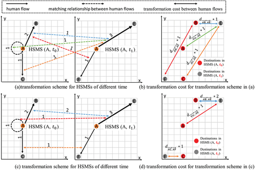
Figure 1 illustrates the HSMS of location A during time slot t, containing three human flows from location A to locations B, C, and D. The thickness of each arrow indicates trip number and length corresponding to trip displacement. The HSMS of location A during time slot t is represented by a set of these three geographical flows. In the planar coordinate system shown in Figure 1, $HSM{S}_{(A,\hspace{0.17em}t)}$ is described as follows:

Figure 1. HSMS graph.

(2) $HSM{S}_{(A,t)}=\left\{\overrightarrow{AB}:\left[\left(4,6\right),\left(7,10\right),2\right],\overrightarrow{AC}:\left[\left(4,6\right),\left(4,1\right),1\right],\overrightarrow{AD}:\left[\left(4,6\right),\left(1,8\right),1\right]\right\}$(2)

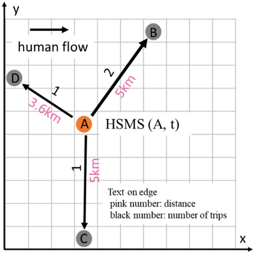
Based on the spatial location and trip flux of human flows, the HSMS describes the spatial and trip number distributions of human mobility. Changes in human mobility at one location are represented by HSMS time series, and differences in human mobility between locations during time slot t are described by HSMS sets. Thus, we quantified the temporal and spatial variations in human mobility using the HSMS. Compared with existing scalar-based representations of human mobility (e.g. trip number and length), the HSMS is more suitable for fully expressing the multidimensional characteristics of human mobility.

3.2 MDI algorithm

The HSMS characterizes human mobility; thus, the differences between HSMSs reflect differences in human mobility. Levenshtein distance is a metric used to assess the similarity between two strings by determining the minimum number of edits required to transform one string into another (Lenvenshtein 1966). Inspired by Levenshtein distance, we introduced the MDI algorithm to measure differences in human mobility by calculating the minimum cost required to transform one HSMS into another. We calculated this minimum transformation cost based on the optimal transport theory. The minimum conversion cost is referred to as the MDI.

To define the transformation between two HSMSs, α and β denote two different HSMSs, each comprising m and n human flows and encompassing N trips. The transformation of α and β refers to the process of transforming N trips in α to N trips in β, making the spatial and trip number distributions of the flows in α and β identical.

3.3. MDI workflow

3.3.1 Pretreatment of HSMSs

First, we offset identical OD flows in two HSMSs. Two OD flows subordinate to two different HSMSs with the same origin, destination, and flow flux have no cost during the HSMS transformation process and can be offset directly. For instance, OD flows AD in Figure 2(a) exists in both HSMS α and β with the same origin, destination, and flow flux; therefore, they can be directly offset and thus removed in α and β. If they contain different flow fluxes, the OD with the smaller flow flux can be removed, and the other OD must eliminate the equivalent flow flux. As shown in Figure 2(a), for OD flows AB subordinate to α and β, the bottom two plots were created after α and β underwent OD flow offset.

Figure 2. MDI workflow.

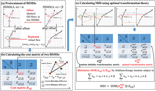
Second, we replenished virtual flow. In practice, trip number contained in two HSMSs often differs. This study introduced the concept of virtual flow, which is a flow with origin and destination at the same location. By adding a virtual flow to an HSMS with fewer trips, both HSMSs can contain the same total trip number. The join of virtual flow tends to increase the transformation cost, thereby merge the flow flux differences into the HSMS transformation cost.

If HSMS α (at location A) and HSMS β contain n1 and n2 trips respectively, and n1 < n2, then a virtual flow can be added to HSMS α, as follows:

(3) $\mathrm{V}\mathrm{i}\mathrm{r}\mathrm{t}\mathrm{u}\mathrm{a}\mathrm{l}\mathrm{f}\mathrm{l}\mathrm{o}\mathrm{w}=\left(coo{r}_A,\hspace{0.17em}coo{r}_A,\mathrm{n}2-\mathrm{n}1\right)$(3)

where $coo{r}_A$ is the coordinate of location A.

3.3.2 Calculating cost matrix of two HSMSs

We use the flow distance metric to measure the transformation cost per unit of trip, that is, flow distance between flows i and j, calculated using Equations (4(4) $d_{ij}=\hspace{0.17em}{d}_{ij}^{\left(o\right)}+\hspace{0.17em}{d}_{ij}^{\left(d\right)}$(4) –6(6) $d_{ij}^{\left(d\right)}=\sqrt{{\left(x_i^{\left(d\right)}-x_j^{\left(d\right)}\right)}^2+\hspace{0.17em}{\left(y_i^{\left(d\right)}-y_j^{\left(d\right)}\right)}^2}$(6) ) (Pei et al. 2020).

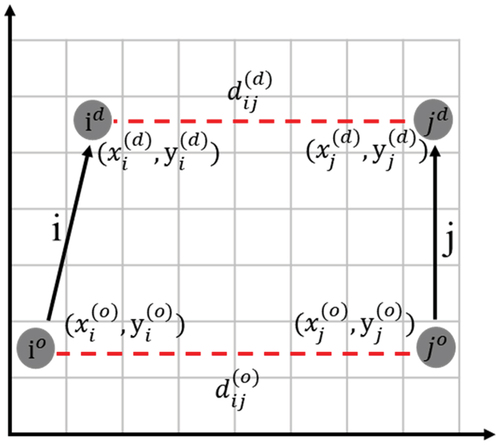
In Figure 3, arrows i and j represent human flows $i^o$ and $i^d$, respectively, which are the origin and destination of flow i; $\left(x_i^o,y_i^o\right)$ are the coordinates of the origin of flow i; $\left(x_i^d,y_i^d\right)$ are the coordinates of the destination of flow i; $d_{ij}^o$is the distance between the origins of flows i and j; $d_{ij}^d$is the distance between the destinations of flows i and j; and distance $d_{ij}$ between flows i and j is the sum of the origin distance $d_{ij}^o$ and destination distance $d_{ij}^d$ of the two human flows.

Figure 3. Flow distance diagram.

(4) $d_{ij}=\hspace{0.17em}{d}_{ij}^{\left(o\right)}+\hspace{0.17em}{d}_{ij}^{\left(d\right)}$(4)

(5) $d_{ij}^{\left(o\right)}=\sqrt{{\left(x_i^{\left(o\right)}-x_j^{\left(o\right)}\right)}^2+\hspace{0.17em}{\left(y_i^{\left(o\right)}-y_j^{\left(o\right)}\right)}^2}$(5)

(6) $d_{ij}^{\left(d\right)}=\sqrt{{\left(x_i^{\left(d\right)}-x_j^{\left(d\right)}\right)}^2+\hspace{0.17em}{\left(y_i^{\left(d\right)}-y_j^{\left(d\right)}\right)}^2}$(6)

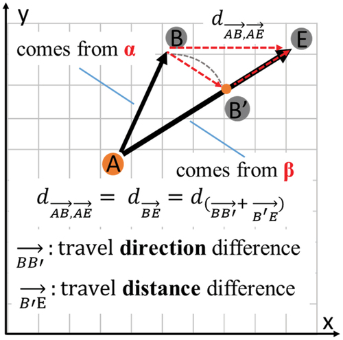
Flow distance is determined using origin and destination distances. It reflects differences in the spatial distribution of population flows and implies changes in flow direction and distance. When comparing flows in temporal variations of human mobility, we considered flows originating from the same location. Flow distance degenerates into the distance between destinations (Figure 4). At different times in the same location, the flows between AB and BE are OD flows. Flow distance, measured using $d_{\underset{AB}{\to }\underset{AE}{\to }}$, considers changes in the flow direction, indicated by $\underset{BB\prime }{\to }$, and variations in flow distance, indicated by $\underset{B\prime E}{\to }$.

Figure 4. Flow distance for temporal variations.

Flow distances between any two flows in different HSMSs can be calculated. If α and β are different HSMSs with m and n flows, respectively, then the flow distances between two HSMSs can form a matrix with m rows and n columns, referred to as the flow distance matrix, as follows:

(7) $D_{\alpha \beta }=\hspace{0.17em}\begin{array}{ccccc}{d}_{11}& \dots & d_{1j}& \dots & d_{1n}\\ \dots & \dots & \dots & \dots & \dots \\ d_{i1}& \dots & d_{ij}& \dots & d_{in}\\ \dots & \dots & \dots & \dots & \dots \\ d_{m1}& \dots & d_{mj}& \dots & d_{mn}\end{array}$(7)

where $d_{ij}$ is the flow distance between the $i_{th}$ human flow of $\alpha$ and $j_{th}$ human flow of $\beta$.

3.3.3 Calculating MDI using the optimal transport theory

3.3.3.1 Optimal transport

Optimal transport describes the problem of m suppliers $\mathrm{S}=\left\{s_i|\mathrm{i}=1,2,\dots \mathrm{m}\right\}$ that need to transport goods to n demanders $\mathrm{D}=\left\{d_j|\mathrm{j}=1,2,\dots \mathrm{n}\right\}$, where s_i denotes the quantity of goods available at the ith supplier and d_j denotes the quantity of goods demanded by the jth demander. The cost of transporting each unit of goods from supplier i to demander j is denoted as d_ij. The objective of optimal transport is to find a transport scheme ${\pi }_{\alpha \beta }=\left\{{\pi }_{ij}|\mathrm{i}=1,2,\dots \mathrm{m};\mathrm{j}=1,2,\dots \mathrm{n}\right\}$ that allows all goods to be transported from suppliers to demanders at the minimum transport cost.

If the transport cost of a route is the same for a round trip, switching the roles of suppliers and demanders has no effect on the total transport cost. By solving a linear programming problem, optimal transport can determine a transport solution that minimizes the total transport cost (Zhang et al. 2020).

3.3.3.2 Transformation matrix

For HSMS α and β, the cost matrix $D_{\alpha ,\beta }$ is determined as described above. Figures 5(a–c) depict HSMS transformation schemes, and Figures 5(b–d) present the corresponding costs. Different transformation schemes incur different costs. MDI calculation determines transformation scheme ${\pi }_{\alpha ,\beta }$ that minimizes the transformation cost between two HSMSs. We considered the determination of the transformation scheme to be an optimal transport problem.

Figure 5. HSMS transformation scheme and cost.

The transformation scheme is represented by the transformation matrix. Let α and β be different HSMSs with m and n flows, respectively, and N trips. To transform α into β, the trips contained in flow i need to be transformed into trips in any of the flows in β. ${\pi }_{ij}$ denotes trip number transformed from the i-th flow in α to j-th flow in β. The matrix of m rows and n columns consisting of ${\pi }_{ij}$ is called the transformation scheme matrix. The transformation scheme matrix determines how human flows belonging to different HSMSs are matched to calculate the final transformation cost, as follows:

(8) ${\pi }_{\alpha \beta }=\hspace{0.17em}\begin{array}{ccccc}{\pi }_{11}& \dots & {\pi }_{1j}& \dots & {\pi }_{1n}\\ \dots & \dots & \dots & \dots & \dots \\ {\pi }_{i1}& \dots & {\pi }_{ij}& \dots & {\pi }_{in}\\ \dots & \dots & \dots & \dots & \dots \\ {\pi }_{m1}& \dots & {\pi }_{mj}& \dots & {\pi }_{mn}\end{array}$(8)

The sum of the elements in row i of the matrix π corresponds to trip number contained in the i-th flow in α, and the sum of the elements in column j corresponds to trip number contained in the j-th flow in β. We satisfy the above requirements for the random initialization of the transformation matrix. The solution of the best transformation scheme is a mathematical optimization problem, described below.

3.3.3.3 Optimal transport for MDI

Based on the optimal transport theory, we considered two HSMSs as a set of suppliers and demanders, each human flow as a supplier or demander, trip number as the quantity of goods, and flow distance as the distance between the supplier and demander. The optimal transport problem is expressed as follows:

(9) $MDI=Min\left(SUM({\pi }_{\alpha \beta }\odot D_{\alpha \beta }\right))$(9)

where ⊙ is the dot product operation of the matrix, SUM is the summation of all elements of the matrix, and Min is the optimization process that minimizes the objective value.

The transformation scheme with the minimum transformation cost ${\pi }_{\alpha \beta }^{opti}$ can be obtained in polynomial time using the Sinkhorn-Knopp iterative solution (Ge et al. 2021).

4. Simulation experiments

To validate the MDI effectiveness, we conducted a simulation experiment comparing four methods: difference of flow flux (DFF) (Fang et al. 2017; Wang, Taylor, and Wu 2014; Zhong et al. 2022); difference of total flow length (DTFL) (Eom, Jang, and Ji 2022; Huang et al. 2021; Zhang et al. 2019); Sørensen – Dice similarity index (SSI), which gauges the magnitude of similarity between predicted and observed human mobility patterns (Schläpfer et al. 2021); and Levenshtein distance for OD matrices (LOD), which quantifies the absolute value of changes in population mobility (Behara, Bhaskar, and Chung 2020).

(10) $DFF=\left|numberoftripsinHSM{S}_1-numberoftripsinHSM{S}_2\right|$(10)

(11) $DTFL=\left|\sum _{i=0}^{n_1}{n}_{f_1}\ast d_{f_1}-\sum _{i=0}^{n_2}{n}_{f_2}\ast d_{f_2}\right|,f_1\in HSM{S}_{1}and{f}_2\in HSM{S}_2$(11)

(12) $\begin{array}{rl}& SSI=2\sum _{f}min\left(n_{f_1},n_{f_2}\right)/\left(\sum _{f_1}{n}_{f_1}+\sum _{f_2}{n}_{f_2}\right),f_1\\ & \in HSM{S}_1,f_2\in HSM{S}_2,f\in HSM{S_1}^{H}SM{S}_2\end{array}$(12)

where $f_1$ and $\hspace{0.17em}{f}_2$ denote human flows in different HSMSs; $n_1$ and $n_2$ are the numbers of flows contained in two HSMSs; $n_{f_1}$and$n_{f_2}$denote trip number contained in human flows $f_1$ and $\hspace{0.17em}{f}_2$; and $d_{f_1}$ and $d_{f_2}$ denote the trip distances corresponding to human flows$\hspace{0.17em}{f}_1$ and $f_2$.

SSI measures the similarity on a scale from 0 to 1, and its complement, 1-SSI, represents the mobility difference, denoted as SSI_c.

(13) $SSI\mathrm{\_}c=1-SSI$(13)

4.1. Temporal variations in human mobility

To verify the advantages of MDI in perceiving the multidimensional characteristics of human mobility, such as trip number, distance, and direction, we conducted a simulation experiment to assess the temporal variations in human mobility. We assumed that the virtual square city had dimensions of 100 km × 100 km. Taking the bottom left corner of the square city as the origin of the coordinates, location A was located at (50 km, 50 km). From t1 to t9, human mobility, including trip number, distance, and direction, at location A changes (Table 1).

Table 1. Human mobility characteristics at different times.

Time	Origin	The number of trips	Range of trip distance	Trip direction
t1	(50,50)	90	(5,15)	360 degree surround around the origin
t2	(50,50)	180	(5,15)	360 degree surround around the origin
t3	(50,50)	360	(5,15)	360 degree surround around the origin
t4	(50,50)	360	(15,25)	360 degree surround around the origin
t5	(50,50)	360	(35,45)	360 degree surround around the origin
t6	(50,50)	360	(35,45)	180 degree surround around the origin
t7	(50,50)	360	(35,45)	90 degree surround around the origin
t8	(50,50)	360	240:(5,15),120:(35,45)	360 degree surround around the origin
t9	(50,50)	90	(35,45)	360 degree surround around the origin

Figure 6(a)shows the flow distribution at location A at different times from t1 to t9. Figures 6(b–f) show the quantitative results for DFF, DTFL, SSI_c, LOD, and MDI, respectively.

Figure 6. Visualization of simulation data and quantitative results of temporal variations in human mobility.

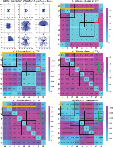
Trip direction and distance at location A at t1, t2, and t3 were the same, whereas trip number differed. The change in trip number from t1 to t3 was greater than that from t1 to t2. Similarly, from t3 to t5 and from t5 to t7, only trip distance and direction at location A differed. As indicated by the black boxes in Figures 6(b–f), DFF distinguished changes from t1 to t3, DTFL distinguished changes from t1 to t3 and t3 to t5, and SSI_c distinguished changes from t1 to t3 and t5 to t7. LOD and MDI distinguished all changes (t1 to t3, t3 to t5, and t5 to t7), with MDI distinguishing variation intensities more clearly.

Furthermore, changes in human mobility increased sequentially from t2 to t7 compared to t1. However, as indicated by the yellow boxes in Figures 6(b–f), only MDI quantification results for t1 maintained a reasonable level of growth from t2 to t7. The quantification results of DFF, DTFL, SSI_c, and LOD at t1 did not change from t4 to t7. The quantification results of DTFL at t1 were nearly identical from t5 to t7 and decreased slightly from t6 to t7. These results demonstrated that only MDI could detect superimposed changes in trip number, distance, and direction.

Moreover, trip number at location A was the same at t4 and t8; however, trip distance changed from t4 to t8, with trip distances increasing or decreasing, indicating divergent changes. As indicated by red boxes in Figure 6(b,c,f), DFF and DTFL quantification results for these divergent changes were close to zero, indicating that DFF and DTFL were ineffective in detecting divergent changes. Conversely, MDI quantification result was 4840 indicating that MDI could detect divergent changes in human mobility. Trip number and distance at location A changed from t3 and t4 to t9, with trip number increasing and distance decreasing, indicating divergent changes. Travel flows decreased by 270 from t3 and t4 to t9, with longer distances at t4 than at t3, leading to more significant variations in mobility. As indicated by the green boxes in Figure 6(d–f), MDI was more effective than SSI_c and LOD in discerning change intensity.

4.2. Spatial differences in human mobility

To verify the effectiveness of the MDI in detecting spatial differences in human mobility, we assumed a virtual square city with dimensions of 100 km × 100 km. Locations A, B, C, and D were located at (50 km, 50 km), (25 km, 75 km), (75 km, 75 km), and (25 km, 25 km), respectively. Thus, B, C, and D were the same distance from A. One hundred outbound trips occurred at each of these four locations, and B, C, and D had the same interaction destination as A with scales of 80%, 50%, and 0%, respectively. Differences in human mobility increased in the order of B, C, and D compared with location A.

Figure 7(a) shows the flow distribution of A, B, C, and D. Figure 7(b–f) show the results of quantifying the spatial differences in human mobility using DFF, DTFL, SSI_c, LOD, and MDI.

Figure 7. Visualization of simulation data and quantitative results of spatial differences in human mobility.

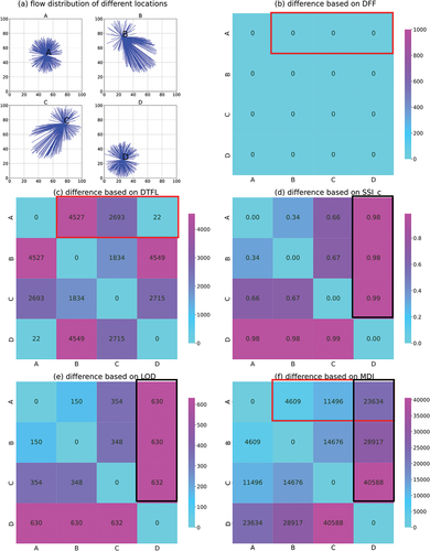
DFF and DTFL were ineffective in quantifying spatial variations in human mobility. Trip number was the same at the four locations; therefore, DFF quantification results were zero, and DFF could not detect any differences. The quantification results of DTFL decreased from 4527 to 22, leading to the erroneous conclusion that the differences in human mobility at locations B, C, and D decreased in that order compared with location A. The quantification results maintained reasonable growth from 4609 to 23,634, which was consistent with the scenario setup. These results demonstrated the effectiveness of the MDI in detecting spatial variations in human mobility.

SSI_c and LOD could not effectively discern the magnitude of disparities in origin distances and destination distributions. A and D have the closest origin distances and most similar destination distributions, resulting in the smallest differences in human mobility. Conversely, C and D had the greatest origin distance and most substantial differences in destination distribution, leading to the most significant disparities in human mobility. Disparities between B and D were intermediate. As indicated by the black-framed areas in Figure 7(d–f), SSI_c (0.98–0.99) and LOD (630–632) identified differences between A, B, C, and D; however, they failed to differentiate the intensity of these differences. Only the MDI (23634–40588) distinguished the varying magnitudes of these differences. These findings underscore the effectiveness of the MDI in integrating spatial flow distribution to quantify spatial variations in human mobility.

5. Case studies

We conducted case studies to investigate the temporal variation and spatial differences in human mobility based on the MDI. We used grid cells as the basic spatial units to examine temporal changes, as this type of units are widely used in urban studies (Sagl, Delmelle, and Delmelle 2014; Yang, Zhao, and Lu 2016). We analyzed the spatial and temporal dependencies of changes in human mobility during the pre-metaphase of the COVID-19 pandemic (December 2019 to January 2020) in Wuhan, China. An area of interest (AOI) refers to regions within an urban environment that attract attention (Hu et al. 2015). To examine spatial differences, we used the AOI as the basic spatial unit and analyzed the effects of spatial heterogeneity of spatial semantics and distance on human mobility.

5.1. Case study 1: temporal variations in human spatial mobility in grid cells

COVID-19 spread worldwide and caused unprecedented public health, social, and economic challenges (Cheng et al. 2020; Jia et al. 2020). Human flow was the main driver of the spread of COVID-19, and urban spaces with highly variable mobility tended to exhibit more frequent changes in their interaction locations, resulting in greater exposure and a higher risk of disease transmission and infection (Gao and Yu 2020; Hu et al. 2021). Spatial and temporal analyses of human mobility variations could help prevent disease spread. Thus, we analyzed spatial and temporal variations in human mobility and effect of social functions on changes in human mobility. We evaluated infection risk in urban spatial units to provide guidance for spatially matching infectious disease prevention and control resources and social activity suggestions for urban residents to avoid infection.

5.1.1 Study area and dataset

Wuhan is a megacity in China with a population of over 10 million and large-scale population movement. Wuhan was the site of the first COVID-19 outbreak in China.

This study used mobile phone data collected by a major telecom operator in Wuhan. The dataset divided Wuhan into 139,145 grid cells with lengths and widths of 250 m. OD flows between cells were recorded at a temporal granularity of days. Data from 10 December 2019, to 31 January 2020, were included.

We compared analyses using the MDI with DFF, DTFL, LOD, and SSI_c in terms of capturing daily mobility pattern changes. Moreover, we examined the MDI’s generalization performance in different cities using open-source OD data for Beijing from May 21st to 27 May 2018, including OD flows between 6651 500-m grid cells (Ren 2022). The average daily OD flows of both mobility datasets were in millions, and the data were fully representative (Table 2).

Table 2. Examples of mobile phone data.

Date	Origin ID	Destination ID	Flow flux
2019/12/10	100172	100719	1
2019/12/10	104327	99004	4
…	…	…	…
2020/1/31	99759	98134	2

Point of interest (POI) geospatial data record the location, name, category, and other information of geographic objects, such as restaurants and hotels. We used 371,653 POI data points from 55 categories to analyze the spatial dependence of human mobility. The POI data for Wuhan were provided by Gaode, a leading provider of navigation, digital maps, and location services in China.

5.1.2. Temporal dependence of variations in human mobility

We computed daily mobility changes in Wuhan and Beijing. The quantitative results for each cell were aggregated to derive human mobility variations for each city (Figure 8).

Figure 8. Daily human mobility variations in Wuhan and Beijing.

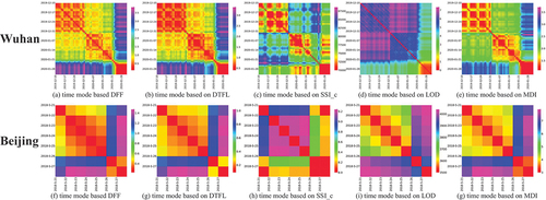
In Figure 8, horizontal and vertical axes represent dates, and cell values indicate changes in human mobility. The MDI effectively captured variations in human mobility between weekdays and weekends. This observation aligned with the notable differences in human activity patterns between the two periods. The primary disparities in human activity between weekdays and weekends were attributed to trip purpose rather than volume or distance. Weekday trips are typically for commuting to and from work, whereas weekend trips are often related to leisure and recreational activities. These trip purposes manifest as changes in interaction locations.

The results from Beijing demonstrated that the MDI provided a superior hierarchy of results compared to the other indicators. This hierarchy was initially evident in weekday-to-weekday comparisons, where both LOD and MDI displayed smaller differences in mobility between consecutive weekdays, gradually increasing the differences in mobility between Mondays and the remaining weekdays. This observation corresponded to the temporal proximity of the population’s travel behaviors, with closer temporal proximity resulting in more similar travel behaviors. Furthermore, the MDI exhibited a nuanced representation of flow differences between weekends and weekdays, emphasizing its ability to discern subtle distinctions between these timeframes. Thus, the MDI effectively captured the influence of temporal characteristics on human mobility, supporting an analysis of mobility driven by regularity.

5.1.3. Spatial dependence of variations in human mobility

To further investigate the spatial distribution of pandemic risk, we calculated the mean MDI value for each 250-m cell in Wuhan (Figure 9(c)). Cells without flow were removed from the map. We divided cells into five classes based on the mean MDI values using the natural breakpoint method. Variations in human mobility increased from Level 1 to Level 5. Figure 9(b) shows the number of cells at each level. Cell number above Level 2 accounted for 8.3% of the total; however, the amount of variation in mobility accounted for 74.19% of the entire city, indicating that most variations in mobility occurred in a few areas in the city. Figure 9(a) shows that, except for several areas, such as Tianhe Airport (location of the aircraft icon), the areas with high variations in mobility above Level 3 were mainly concentrated within the third ring road in Wuhan City. We labeled the landmarks in cells at Level 5 in Figure 9(c) according to the POI data. The highest variations in human mobility were concentrated near railway stations, large commercial centers, and tertiary level A hospitals.

Figure 9. Spatial distribution and grid number of human mobility variations.

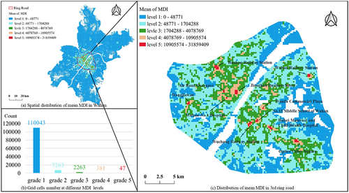
We matched each POI to 250 m grid cells by spatial join operation. Based on the matching relationship in space, we analyzed the contributions of POI categories to variations in mobility and explored the effect of urban elements on variation intensity High variations indicated high infection risk.

Based on the results shown in Figure 9, we reclassified cells into three variation types: high (Levels 4 and 5), medium (Levels 2 and 3), and low (Level 1). We defined the POI contribution index $C_{pg}$ to quantify the contribution of POI type p to the variation in mobility level g, as follows:

(14) $C_{pg}=\frac{P_{rate}}{G_{rate}}$(14)

where $P_{rate}=\frac{N_{p,g}}{N_{p,total}}$; $G_{rate}=\frac{N_g}{N_{total}}$; p denotes the POI category; g denotes the variation in the mobility level;$N_{p,g}$ is the number of POIs in category p in grid cells with variation in mobility level g;$N_{p,total}$ denotes the total number of POIs in category p;$N_g$ denotes the number of grid cells with variation in mobility level g; and $N_{total}$ denotes the total number of grid cells.

We followed the quadrat analysis method in spatial point pattern analysis to assess the clustering of POIs in grids of different mobility variation levels. The quadrat analysis method compares the actual point density within a region with that of a hypothesized standard distribution (usually a random distribution), indicating the degree of clustering in the actual point distribution. In the calculation formula for $C_{pg}$, $G_{rate}$ represents the global standard distribution density of p-type POIs, and $P_{rate}$ represents the actual distribution density of p-type POIs within g-level grids. The clustering degree of p-type POIs in g-level grids is explained based on $C_{pg}$. A higher $C_{pg}$ value indicates that the distribution of p-type POIs is more concentrated in grid cells with g-level mobility variation. This implies that p-type POIs contribute more to the g-level mobility variation, suggesting a higher spatial dependency of the g-level mobility variation on p-type POIs.

Table 3 shows the POI categories with the top 10 contributions to the three types of variations in mobility. The values represent the POI contribution index $C_{pg}$. Higher $C_{pg}$ values indicate a greater contribution of the POI category p to the g grade of the variations in mobility. The POI types with high contributions to different grades of mobility variation differed significantly. The first type of POI was characterized by service scope and scarcity. The POI categories are shown in red in Table 3, where the grid cells with high variations in mobility include stations, airports, and tertiary Level A hospitals. POIs in these categories were few and served the entire city. Conversely, specialist hospitals, farmers’ markets, and community service centers in cells with moderate mobility variations tended to serve localized areas of the city and were more numerous. In addition, in cells with low mobility variations, bus stops, public facilities (e.g. public toilets and newsagents), and petrol stations were ubiquitous and served small areas. The second type of POI was characterized by visit frequency and intensity of human activity. These POI types are marked in blue in Table 3. They included clothing stores and restaurants in areas with high variation in mobility. These POI categories were frequently visited, whereas POI categories such as auto repair shops and motor vehicle services in areas with moderate mobility variations had lower visit frequencies. Conversely, agricultural bases, villages, and other POIs had almost no public service functions and the lowest visit frequencies. Therefore, scarce public resources with a wide range of services and areas with a high intensity of visits and activities tended to have higher mobility variations.

Table 3. POI categories with top 10 contributions.

Order	Grade 1 (low variation in mobility)	Grade 2 (medium variation in mobility)	Grade 3 (high variation in mobility)
1	(Agricultural Base, 0.943)	(‘Auto Repair’, 10.464)	(‘Railway Station’, 128.639)
2	(‘Village’, 0.911)	(‘Special Hospital’, 10.153)	(‘Clothing Store’, 73.264)
3	(‘Port & Marina’, 0.635)	(‘Farmers Market’, 10.146)	(‘Foreign Food Restaurant’, 72.304)
4	(‘Factory’, 0.587)	(‘Motor Vehicle Services’, 9.969)	(‘Airport’, 72.094)
5	(‘Tourist Attraction’, 0.524)	(‘Community Center’, 9.872)	(’ Tertiary Level-A Hospitals ’, 64.251)
6	(‘Bus Station’, 0.523)	(‘Bank’, 9.839)	(‘Shopping Plaza’, 64.016)
7	(‘Coach Station’, 0.509)	(‘Media Organization’, 9.788)	(‘Luxury Hotel’, 60.764)
8	(‘Villa’, 0.483)	(‘Chinese Food Restaurant’, 9.762)	(‘Commercial Street’, 53.755)
9	(‘Public Facility’, 0.434)	(‘Home Building Materials Market’, 9.745)	(‘Leisure Food Restaurant’, 50.439)
10	(‘Filling Station’, 0.386)	(‘Arts Organization’, 9.742)	(‘Fast Food Restaurant’, 49.072)

Furthermore, we summed the contributions of POIs to different types of variations in mobility (Table 4). These contributions could be used to identify COVID-19-infection risk. Based on data released by the public and official websites of the Wuhan Municipal Commission, Zhang et al. (2022) prepared a complete heat map of the distribution of COVID-19 from the outbreak to 28 February 2020. The pandemic was concentrated at Wuhan Railway Station and the urban center, with residential areas forming the core, a dense road transport network, and complex mobile population. Moreover, they found increased infections at hospitals, hotels, and subway stations. In our study, railway stations, tertiary level-A hospitals, upscale hotels, and subway stations ranked first, fifth, seventh, and 13th, respectively, similar to previous findings.

Table 4. Contributions to variations in mobility among 55 types of POIs.

Order	POI type	Cp,g	Order	POI type	Cp,g
1	Railway Station	134.102	29	Science & Technology Exhibition Hall	39.663
2	Clothing Store	82.106	30	General Hospital	37.905
3	Foreign Food Restaurant	81.272	31	Residential Quarter	37.042
4	Airport	79.808	32	School	35.318
5	Tertiary Level-A Hospitals	73.921	33	Research Institution	34.667
6	Shopping Plaza	72.372	34	Chain Supermarket	34.434
7	Luxury Hotel	69.231	35	Convenience Store	33.096
8	Commercial Street	63.288	36	Street Furniture	32.935
9	Leisure Food Restaurant	60.106	37	Farmers Market	32.641
10	Fast-Food Restaurant	58.593	38	Coach Station	32.22
11	General Merchandise	56.472	39	Governmental & Social Organization	31.634
12	Financial & Economic Insurance	55.706	40	Health Center	26.895
13	Subway Station	54.832	41	Clinic	26.65
14	Budget Hotel	54.82	42	Park & Square	26.107
15	Home Electronics	54.183	43	Home Building Materials Market	24.877
16	Arts Organization	50.949	44	Logistics Service	23.572
17	Beauty and Hairdressing Store	50.185	45	Filling Station	20.454
18	Special Hospital	49.282	46	Motor Vehicle Services	20.111
19	Media Organization	49.281	47	Tourist Attraction	19.433
20	Bank	47.843	48	Auto Repair	17.01
21	Sports & Recreation Places	47.056	49	Auto Dealers	16.771
22	Chinese Food Restaurant	44.369	50	Port & Marina	15.986
23	Public Facility	42.596	51	Bus Station	15.44
24	Parking Lot	42.555	52	Factory	11.614
25	Company	42.519	53	Villa	10.397
26	Job Centre	41.501	54	Agricultural Base	4.025
27	Community Center	40.886	55	Village	3.592
28	Business Office Building	39.988

Different types of POIs with similar social functions differed significantly in in mobility variations. For instance, all three types of POIs in red provided long-distance travel services; however, mobility variations were significantly higher at the railway station than airport, and at the airport than coach station. Thus, infection risk was higher at the railway station than at the airport, and at the airport than at the coach station, which could relate to resource scarcity and social activity intensity. Urban facilities with high resource scarcity tend to attract a wider range of residents, and high social activity intensity leads to intensive crowd contact, thereby increasing the risk of infection. Similar conclusions are drawn from the data in Table 4. The risk of infection in medical spaces (indicated in blue) followed the order of Level A hospitals > specialist hospitals > general hospitals > health centers and clinics. The risk of infection in entertainment and leisure spaces (indicated in yellow) followed the order of commercial streets > sports and recreation facilities > parks and squares. The risk of infection in short-distance travel spaces (indicated in green) followed the order of subway stations > bus stations.

5.2. Case study 2: spatial differences in human mobility in AOIs

The impact of spatial semantics and distance on human mobility is crucial for urban planning and functional optimization (Tao et al. 2019). We evaluated the MDI by exploring whether spatial difference in human mobility reflected the heterogeneous effect of spatial semantics and distance decay effect of human mobility similarity.

Area of interest (AOI) is a geographical entity that represents the typical urban function of a corresponding urban space (Hu et al. 2015; Ma et al. 2019). The semantic category information inherent in an AOI provides a detailed description of local land-use functions. For instance, an AOI categorized as a hospital indicates that the land-use function in the area is medical services. Investigating the differences in mobility across various semantic types of AOIs can enhance our understanding of the role of spatial semantics and constraining effect of distance on human mobility. Therefore, we employed the AOI as the basic spatial unit to quantify spatial differences in human mobility and verified the heterogeneous roles of spatial semantics in differences in human mobility. Furthermore, we examined the impact of distance on the spatial differences in human mobility within the same semantic types of AOIs.

5.2.1. Study area and data sets

We selected Wuchang District in Wuhan as the study area, as it is the seat of the People’s Government in Hubei Province, has a population of over one million, and is one of the main urban areas in Wuhan. We included 1,050 AOIs in 13 categories. We used mobile phone location data to generate mobility data between the AOIs. AOI and mobile phone location data were obtained from a big data advertising and operations company in Shanghai, China.

The mobile phone location data consisted of more than 110 million records collected between April 8 and 24 May 2018, in Wuchang District. Each record contained information such as longitude, latitude, and timestamp, with a location positioning accuracy of 10 m and time resolution of minutes. We utilized the scikit-mobility Python library to extract user stay points. This library employs a time-distance rule to identify user stay points, with stay points being consecutive points not exceeding a specified distance threshold within a certain time interval threshold. Default library thresholds for time and space were 20 min and 200 m, respectively. Due to the high spatial resolution of the mobile positioning data, we used a stringent stay threshold of 15 min and 50 m. We generated 3.84 million OD flow data points based on the relationship between dwell points and spatial extent of AOIs.

5.2.2. Heterogeneous effect of spatial semantics

Spatial units with similar social semantics on the local spatial scale perform similar social functions; thus, human mobility is similar. Therefore, at a local spatial scale, such as a traffic analysis zone (TAZ), which is a closed area enclosed by a road network, the difference in mobility between AOIs with the same type of spatial semantics should be smaller than that between AOIs with different types of spatial semantics.

To validate the MDI’s ability to reflect the impact of spatial semantics on human mobility, we evaluated the differences in mobility for different AOIs within the same TAZ using five indicators: DFF, DTFL, SSI_c, LOD, and MDI. We grouped AOIs by semantic type and calculated the category mean value of mobility difference (CMVMD) between types of spatial semantics. The CMVMD indicates the magnitude of the difference in human mobility between AOI categories, with higher CMVMD values indicating greater differences in human mobility. The results are presented in Table 5.

Table 5. Top two CMVMDs in each spatial semantic.

Semantic type	DFL	DTFL	SSI	LOD	MDI
Shopping (Sh)	(‘SL,’ 0.066) (‘Sh,’ 0.128)	(‘Sh,’ 0.13) (‘SL,’ 0.164)	(Sh, 0.227) (TA,0.949)	(Sh, 0.267) (TA,0.949)	(‘Sh,’ 0.143) (‘SL,’ 0.486)
Food & Beverage (FB)	(‘GSO,’ 0.117) (‘AS,’ 0.259)	(‘AS,’ 0.301) (‘AuS,’ 0.407)	(‘AS,’ 0.967) (‘AuS,’ 0.980)	(‘AS,’ 0.942) (‘AuS,’ 0.970)	(‘GSO,’ 0.481) (‘AS,’ 0.557)
Medical Services (MS)	(‘MS,’ 0.117) (‘GSO,’ 0.141)	(‘GSO,’ 0.041) (‘MS,’ 0.115)	(‘MS,’ 0.318) (Sh, 0.966)	(‘MS,’ 0.318) (‘GSO,’ 0.973)	(‘MS,’ 0.21) (‘GSO,’ 0.539)
Government and Social Organization (GSO)	(‘FB,’ 0.117) (‘MS,’ 0.141)	(‘MS,’ 0.041) (‘GSO,’ 0.189)	(‘GSO,’ 0.545) (‘RB,’ 0.979)	(‘GSO,’ 0.537) (‘RB,’ 0.972)	(‘GSO,’ 0.352) (‘FB,’ 0.481)
Residential Building (RB)	(‘SL,’ 0.3) (‘TS,’ 0.377)	(‘SL,’ 0.25) (‘TS,’ 0.367)	(‘RB,’ 0.890) (‘FIS,’ 0.927)	(‘RB,’ 0.887) (‘FIS,’ 0.920)	(‘SL,’ 0.582) (‘RB,’ 0.614)
Accommodation Services (AS)	(‘AS,’ 0.141) (‘FB,’ 0.259)	(‘AS,’ 0.166) (‘DLS,’ 0.193)	(‘AS,’ 0.400) (‘TS,’ 0.951)	(‘AS,’ 0.400) (‘FB,’ 0.943)	(‘AS,’ 0.279) (‘FB,’ 0.557)
Science Culture and Education (SCE)	(‘SCE,’ 0.209) (‘FB,’ 0.381)	(‘DLS,’ 0.123) (‘SCE,’ 0.202)	(‘SCE,’ 0.454) (‘TA,’ 0.969)	(‘SCE,’ 0.456) (‘TA,’ 0.976)	(‘SCE,’ 0.326) (‘Sh,’ 0.694)
Tourist Attraction (TA)	(‘AuS,’ 0.075) (‘TA,’ 0.106)	(‘AuS,’ 0.074) (‘TA,’ 0.096)	(‘TA,’ 0.196) (‘RB,’ 0.936)	(‘TA,’ 0.211) (‘SL,’ 0.907)	(‘TA,’ 0.13) (‘AuS,’ 0.422)
Finance and Insurance Services (FIS)	(‘SL,’ 0.363) (‘Sh,’ 0.419)	(‘SL,’ 0.369) (‘RB,’ 0.462)	(‘RB,’ 0.927) (‘SL,’ 0.980)	(‘RB,’ 0.920) (‘SL,’ 0.965)	(‘SL,’ 0.621) (‘Sh,’ 0.662)
Sports and Leisure (SL)	(‘Sh,’ 0.066) (‘RB,’ 0.3)	(‘Sh,’ 0.164) (‘RB,’ 0.25)	(‘TA,’ 0.953) (‘RB,’ 0.966)	(‘TA,’ 0.907) (‘RB,’ 0.956)	(‘Sh,’ 0.486) (‘RB,’ 0.582)
Automobile Service (AuS)	(‘AuS,’ 0.067) (‘TA,’ 0.075)	(‘TA,’ 0.074) (‘AuS,’ 0.095)	(‘AuS,’ 0.277) (‘FB,’ 0.980)	(‘AuS,’ 0.279) (‘FB,’ 0.970)	(‘AuS,’ 0.182) (‘TA,’ 0.422)
Daily Life Services (DLS)	(‘AS,’ 0.282) (‘AuS,’ 0.297)	(‘SCE,’ 0.123) (‘AS,’ 0.193)	(‘RB,’ 0.969) (‘AS,’ 0.983)	(‘AS,’ 0.969) (‘RB,’ 0.976)	(‘AuS,’ 0.502) (‘AS,’ 0.592)
Transportation Services (TS)	(‘MS,’ 0.295) (‘RB,’ 0.377)	(‘MS,’ 0.243) (‘RB,’ 0.367)	(‘AS,’ 0.951) (‘RB,’ 0.961)	(‘RB,’ 0.951) (‘AS,’ 0.951)	(‘RB,’ 0.623) (‘AuS,’ 0.64)

(15) $CMVMD=\frac{{\sum }_{i=0}^{n_{c1,\hspace{0.17em}c2}}mobility\hspace{0.17em}difference\hspace{0.17em}\left(AO{I}_{c1},\hspace{0.17em}AO{I}_{c2}\right)}{n_{c1,\hspace{0.17em}c2}}$(15)

where c1 and c2 are AOI categories; $AO{I}_{c1}$和$AO{I}_{c2}$ are AOIs with semantic categories c1 and c2, respectively; and $n_{c1,c2}$ represent the number of AOI pairs in the same TAZ in categories c1 and c2, respectively.

We assessed the sensitivity of five indicators to variations in human mobility. The criterion was having minimal differences in human mobility between AOIs of the same semantic type. In eight types, AOIs of the same semantic types occurred together within the same TAZ. Table 5 presents the top two semantic categories with minimum mobility differences for each metric, with bold indicating mobility difference results in the same AOI category. SSI_c and LOD achieved the minimum mobility differences in the same semantic category for all eight considered categories. The MDI exhibited minimum mobility differences in seven categories in the same semantic category, whereas DFF and DTFL achieved this in four and two categories, respectively.

SSI_c and LOD were the most effective in identifying minor differences in human mobility between AOIs with the same spatial semantics. MDI was slightly less effective than SSI_c and LOD but significantly more effective than DFF and DTFL.

Based on the city primacy index (Jefferson 1939), the mobility difference semantic category index (MDSCI) was defined to reflect the sensitivity of different indicators to differences in human mobility caused by spatial semantic differences.

(16) $\mathrm{M}\mathrm{D}\mathrm{S}\mathrm{C}\mathrm{I}=\frac{\mathrm{C}\mathrm{M}\mathrm{V}\mathrm{M}{\mathrm{D}}_{min}}{\mathrm{C}\mathrm{M}\mathrm{V}\mathrm{M}{\mathrm{D}}_{same}}$(16)

where $\mathrm{C}\mathrm{M}\mathrm{V}\mathrm{M}{\mathrm{D}}_{min}$ is the minimum CMVMD between AOI categories, and $\mathrm{C}\mathrm{M}\mathrm{V}\mathrm{M}{\mathrm{D}}_{same}$ is the CMVMD between AOI categories. Higher MDSCI values indicate greater differences between $\mathrm{C}\mathrm{M}\mathrm{V}\mathrm{M}{\mathrm{D}}_{min}$ and $\mathrm{C}\mathrm{M}\mathrm{V}\mathrm{M}{\mathrm{D}}_{same}$, and this indicator is sensitive to differences in human mobility caused by spatial semantics (Figure 10).

Figure 10. MDSCIs for eight types of spatial semantics.

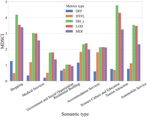
Figure 10 shows that among the eight spatial semantic types, the MDSCI values for the MDI, LOD, and SSI_c were significantly higher than those for the DFF and DTFL. A mean MDSCI score was calculated for each indicator. The mean MDSCI for the MDI, LOD, and SSI_c were 2.246, 2.713, and 2.856, respectively, which were significantly higher than 0.727 and 1.063 for the DFF and DTFL, respectively. LOD and SSI_c were the most sensitive, with the MDI producing results comparable to LOD and SSI_c but with lower sensitivity. The DFF and DTFL exhibited the poorest sensitivity. The computation of mobility differences in LOD and SSI_c is similar to matching interactive destinations, where changes in interactive destinations lead to drastic changes in the results. Conversely, when destinations change, the MDI quantifies mobility differences based on the magnitude of changes in spatial distribution. Consequently, these changes are gradual. However, DFF and DTFL focus on flow volume and distance and are ineffective in quantifying the impact of semantics on interactive destinations.

5.2.3. Effects of spatial distance on spatial differences

We analyzed the relationship between distance and differences in human mobility among AOIs with the same semantic types. We grouped AOIs based on the eight semantic types presented in Figure 8 and calculated the differences in mobility between each pair of AOIs using the DFF, DTFL, SSI_c, LOD, and MDI. The magnitude of the mobility difference was affected by the mobility scale of the AOIs; AOIs with larger flows tended to exhibit greater differences in mobility. Thus, we defined the rate of mobility difference and mobility scale as the relative mobility difference (RMD) to investigate the relationship between spatial distance and differences in spatial mobility. This definition excludes the influence of the mobility scale on mobility differences, as follows:

(17) $RM{D}_{a,b}=\hspace{0.17em}\frac{M{D}_{a,b}}{S_a+S_b}$(17)

where $RM{D}_{a,b}$ is the relative mobility difference between AOIs a and b; $M{D}_{a,b}$ is the mobility difference between AOI a and b represented by DFF, DTFL, LOD, and MDI, respectively; $S_a$ is the mobility scale of AOI a; and $S_b$ is the mobility scale of AOI b. The quantity dimensions for the MDI and DTFL were set as the product of the distance and flow flux, and the total flow length was used to denote the mobility scale. Total flux denoted the mobility scale of the DFF. The SSI_c represented the relative changes in mobility, and no further processing was conducted.

Figure 11 depicts the relationship between the Euclidean distance of two AOIs and differences in human mobility between different AOI categories. The horizontal axis represents the Euclidean distance between AOIs with the same semantic type. The vertical axis represents the relative mobility difference between two AOIs calculated using the five metrics. The red lines represent linear fits to the scatter plots, and the corresponding Pearson correlation coefficients are displayed. The relationships between mobility distances and differences using the DFF and DTFL appeared random, with correlation coefficients between −0.092 and 0.122. The DFF and DTFL treat human mobility as a scalar value, thereby disregarding the spatial distribution of human flows. Thus, they cannot accurately reflect the trends in human mobility with spatial distance. SSI_c and LOD results revealed that AOIs in close proximity exhibited low mobility differences, whereas AOIs at greater distances demonstrated high mobility differences. The correlation coefficients ranged from 0.147 to 0.397. However, the quantitative outcomes exhibited sudden changes in distance. Few AOI pairs exhibited flow similarity, whereas the majority of AOI pairs showed flow differences close to one. Conversely, human mobility differences based on the MDI tended to increase with distance, and the correlation coefficients between spatial flow differences and spatial distances were between 0.709 and 0.829. This was consistent with geography first law: “Everything’s related to everything else, but near things are more related than distant things” (Tobler 1970). Our findings suggest that the MDI can capture the effects of spatial semantics and distance on differences in human mobility and provide scientific results for human mobility analysis.

Figure 11. Relationships between differences in human mobility and distance for AOI categories.

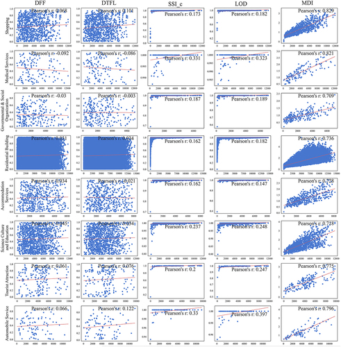
In addition, the correlation coefficients for mobility differences calculated using the MDI varied between AOI categories, reflecting different distance tolerances of the population for different urban functions. For instance, the correlation coefficient for shopping AOIs was 0.829, which was significantly higher than the 0.709 for government and social organization AOIs. This difference indicated that the population had a higher distance tolerance for government and social organization functions than for shopping functions, implying that shopping functions should be situated closer to places of residence or work but at greater distances. Combined with refined data on the classification of urban functions, this can provide detailed and precise insights into planning urban functions.

6. Conclusions and future work

This study proposed the MDI to measure temporal and spatial variations in human mobility. Compared with four frontier methods, our simulation-based experiments confirmed two advantages of the MDI: (1) detecting superimposed and divergent changes in the multidimensional characteristics of human mobility and (2) integrating the spatial location of human flows to quantify spatial variations in human mobility.

The ability of the MDI to detect changes in a population’s travel destinations was demonstrated by showing a clear difference in mobility between weekdays and weekends. Urban spatial elements affected changes in human mobility during the COVID pandemic. Areas with high variations in mobility should be prioritized for infectious disease prevention and control resources, and citizens should reduce travel to these areas to reduce the risk of infection. Our findings were in line with those of previous studies on the risk of COVID-19 infection, demonstrating the accuracy of the MDI in detecting geographical phenomena associated with human mobility.

Moreover, compared to four frontier methods, the MDI demonstrated higher sensitivity in detecting the impact of spatial semantics and spatial distance on human mobility. The quantitative results of the MDI confirmed that similar spatial functions at the local scale promoted similar human mobility and the distance decay effect of similarity. In addition, the results indicated that urban residents had different distance tolerances for different urban functions and that urban functions with lower distance tolerances should be located closer to where citizens live or work.

The MDI considers the spatial distribution of human mobility and accounts for various dimensions of population mobility. Consequently, the MDI is expected to enhance research and application of population mobility in several areas. First, this method can identify multidimensional differences in population flows, including flow direction, flux, and distance. This provides a detailed and comprehensive assessment index for evaluating population flow generation algorithms by accurately measuring the disparities between predicted population flow results and actual flow data. Moreover, the MDI computational process is differentiable. With the advancement of OD flow generation algorithms that rely on deep learning methods, the MDI is likely to be employed as a loss function in deep learning techniques. This would facilitate imposing constraints on human mobility modeling and improve the performance of population flow prediction algorithms. Second, the MDI can be extended by replacing the flow distance in the cost matrix with other attributes. For instance, replacing flow distance with land-use functional differences in destinations could reflect changes in travel purpose and interest over time, which could reveal the driving forces behind human mobility in urban areas. Finally, population mobility similarity could function as a foundation for defining administrative units, such as the TAZ; thus, the MDI could aid in demarcating management units in urban transportation and related areas.

Two limitations of the MDI need to be considered. First, while the MDI captures differences in the multidimensional characteristics of human mobility, identifying aspects of human mobility that differ based on flow flux, total flow length, and other factors is also crucial. These indicators are complementary and can be used together to quantify the differences in human mobility. Second, the MDI has high computational complexity due to iterative optimization in the computational processes. Although the Sinkhorn-Knopp iteration solves the optimization process expediently and effectively, the MDI has a greater computational cost than straightforward metrics, such as differences in flow flux. The time required for computation should be factored into real-time applications.

Investigating quantitative indicators of differences in human mobility is a fundamentally important task in urban human mobility modeling. The present study considered analytical tasks, such as temporal and spatial variations in human mobility; analysis units, such as grid cells and AOIs; scenarios, such as short-term pandemic outbreaks and daily city operation; and data types, such as simulated data, mobile phone signaling, and location data; however, our experiments were limited to Wuhan and Beijing. Experimental validations and comparisons of the results could be conducted in other cities in the future to verify the generalizability of the method. In addition, regularity-driven simulations and predictions of human mobility could be conducted by combining urban spatial semantics and causal inference methods based on the quantitative results for human mobility differences.

Glossary

MDI	=	Mobility Difference Index
HSMS	=	Human Spatial Mobility Situation
DFF	=	Difference of Flow Flux
DTFL	=	Difference of Total Flow Length
POI	=	Point of Interest
AOI	=	Area of Interest
TAZ	=	Traffic Analysis Zone
CMVMD	=	Category Mean Value of Mobility Difference
MDSCI	=	Mobility Difference Semantic Category Index
RMD	=	Relative Mobility Difference

Disclosure statement

No potential conflict of interest was reported by the author(s).

Data availability statement

Data not available due to legal restrictions.

Due to the nature of this research, participants of this study did not agree for their data to be shared publicly, so supporting data is not available.

Additional information

Funding

The work was supported by the National Natural Science Foundation of China [U20A2091]; National Natural Science Foundation of China [41930107]; National Natural Science Foundation of China [41771426].

References

- Amini, A., K. Kung, C. Kang, S. Sobolevsky, and C. Ratti. 2014. “The Impact of Social Segregation on Human Mobility in Developing and Industrialized Regions.” EPJ Data Science 3 (1). https://doi.org/10.1140/epjds31.
- Behara, K. N. S., A. Bhaskar, and E. Chung. 2020. “A Novel Approach for the Structural Comparison of Origin-Destination Matrices: Levenshtein Distance.” Transportation Research Part C: Emerging Technologies 111:513–23. https://doi.org/10.1016/j.trc.2020.01.005.
- Brockmann, D., L. Hufnagel, and T. Geisel. 2006. “The Scaling Laws of Human Travel.” Nature 439 (7075): 462–465. Nature Publishing Group. https://doi.org/10.1038/nature04292.
- Cai, L., J. Xu, J. Liu, T. Ma, T. Pei, and C. Zhou. 2019. “Sensing Multiple Semantics of Urban Space from Crowdsourcing Positioning Data.” Cities 93 (October): 31–42. Elsevier Ltd. https://doi.org/10.1016/j.cities.2019.04.011.
- Cheng, C., T. Zhang, C. Song, S. Shen, Y. Jiang, and X. Zhang. 2020. “The Coupled Impact of Emergency Responses and Population Flows on the COVID-19 Pandemic in China.” GeoHealth 4 (12): John Wiley and Sons Inc. https://doi.org/10.1029/2020GH000332.
- de Andrade, S. C., J. Porto de Albuquerque, C. Restrepo-Estrada, R. Westerholt, C. Augusto Morales Rodriguez, E. Mario Mendiondo, and A. Cláudio Botazzo Delbem. 2022. “The Effect of Intra-Urban Mobility Flows on the Spatial Heterogeneity of Social Media Activity: Investigating the Response to Rainfall Events.” International Journal of Geographical Information Science 36 (6): 1140–1165. Taylor and Francis Ltd. https://doi.org/10.1080/13658816.2021.1957898.
- Elarde, J., J. Seok Kim, H. Kavak, A. Züfle, T. Anderson, and I. Benenson. 2021 November. “Change of Human Mobility During COVID-19: A United States Case Study.” PloS One 16 (11): e0259031. Public Library of Science. https://doi.org/10.1371/journal.pone.0259031.
- Eom, S., M. Jang, and N. S. Ji. 2022. “Human Mobility Change Pattern and Influencing Factors During COVID-19, from the Outbreak to the Deceleration Stage: A Study of Seoul Metropolitan City.” The Professional Geographer 74 (1): 1–15. Routledge. https://doi.org/10.1080/00330124.2021.1949729.
- Fang, Z., X. Yang, Y. Xu, S. Lung Shaw, and L. Yin. 2017. “Spatiotemporal Model for Assessing the Stability of Urban Human Convergence and Divergence Patterns.” International Journal of Geographical Information Science 31 (11): 2119–2141. Taylor and Francis Ltd. https://doi.org/10.1080/13658816.2017.1346256.
- Gao, X., and J. Yu. 2020. “Public Governance Mechanism in the Prevention and Control of the COVID-19: Information, Decision-Making and Execution.” Journal of Chinese Governance 5 (2): 178–197. Taylor and Francis Ltd. https://doi.org/10.1080/23812346.2020.1744922.
- Ge, Z., S. Liu, Z. Li, O. Yoshie, and J. Sun. 2021. “OTA: Optimal Transport Assignment for Object Detection,” March. http://arxiv.org/abs/2103.14259.
- Gibbs, H., Y. Liu, C. A. B. Pearson, C. I. Jarvis, C. Grundy, B. J. Quilty, C. Diamond, et al. 2020. “Changing Travel Patterns in China During the Early Stages of the COVID-19 Pandemic.” Nature Communications 11 (1): Nature Research https://doi.org/10.1038/s41467-020-18783-0.
- González, M. C., A. H. César, and A. László Barabási. 2008. “Understanding Individual Human Mobility Patterns.” Nature 453 (7196): 779–782. Nature Publishing Group. https://doi.org/10.1038/nature06958.
- Hasan, S., C. M. Schneider, S. V. Ukkusuri, and M. C. González. 2013. “Spatiotemporal Patterns of Urban Human Mobility.” Journal of Statistical Physics 151 (1–2): 304–318. Springer Science and Business Media, LLC. https://doi.org/10.1007/s10955-012-0645-0.
- Hu, T., S. Wang, B. She, M. Zhang, X. Huang, Y. Cui, J. Khuri, et al. 2021. “Human Mobility Data in the COVID-19 Pandemic: Characteristics, Applications, and Challenges.” International Journal of Digital Earth 14 (9): 1126–1147. Taylor and Francis Ltd. https://doi.org/10.1080/17538947.2021.1952324.
- Hu, Y., S. Gao, K. Janowicz, B. Yu, W. Li, and S. Prasad. November 2015. “Extracting and Understanding Urban Areas of Interest Using Geotagged Photos.” Computers, Environment and Urban Systems 54:240–254. Elsevier Ltd. https://doi.org/10.1016/j.compenvurbsys.2015.09.001.
- Huang, X., Z. Li, Y. Jiang, X. Ye, C. Deng, J. Zhang, and X. Li. 2021. “The Characteristics of Multi-Source Mobility Datasets and How They Reveal the Luxury Nature of Social Distancing in the U.S. During the COVID-19 Pandemic.” International Journal of Digital Earth 14 (4): 424–442. Taylor and Francis Ltd. https://doi.org/10.1080/17538947.2021.1886358.
- Huang, X., Z. Li, J. Lu, S. Wang, H. Wei, and B. Chen. 2020. “Time-Series Clustering for Home Dwell Time During COVID-19: What Can We Learn from It?” ISPRS International Journal of Geo-Information 9 (11): 675. MDPI AG. https://doi.org/10.3390/ijgi9110675.
- Jefferson, M. 1939. “The Law of the Primate City.” Geographical Review 79 (2): 226–232. https://doi.org/10.2307/215528.
- Jia, J. S., X. Lu, Y. Yuan, G. Xu, J. Jia, and N. A. Christakis. 2020. “Population Flow Drives Spatio-Temporal Distribution of COVID-19 in China.” Nature 582 (7812): 389–394. Nature Research. https://doi.org/10.1038/s41586-020-2284-y.
- Jiang, S., W. Guan, W. Zhang, X. Chen, and L. Yang. 2017. “Human Mobility in Space from Three Modes of Public Transportation.” Physica A: Statistical Mechanics and Its Applications 483 (October): 227–238. Elsevier B.V. https://doi.org/10.1016/j.physa.2017.04.182.
- Karamshuk, D., C. Boldrini, M. Conti, and A. Passarella. 2011. “Human Mobility Models for Opportunistic Networks.” IEEE Communications Magazine. https://doi.org/10.1109/MCOM.2011.6094021.
- Kraemer, M. U. G., C.-H. Yang, B. Gutierrez, C.-H. Wu, B. Klein, D. M. Pigott, Open COVID-19 Data, et al. 2020. “The Effect of Human Mobility and Control Measures on the COVID-19 Epidemic in China.” https://www.science.org.
- Lenvenshtein, V. I. 1966. “Binary Codes Capable of Correcting Deletions Insertions, and Reversals.” Soviet Physics Doklady 10 (8): 707–710.
- Ma, H., Y. Meng, H. Xing, and C. Li. 2019. “Investigating Road-Constrained Spatial Distributions and Semantic Attractiveness for Area of Interest.” Sustainability (Switzerland) 11 (17): 4624. MDPI. https://doi.org/10.3390/su11174624.
- McInerney, J., S. Stein, A. Rogers, and N. R. Jennings. 2013. “Breaking the Habit: Measuring and Predicting Departures from Routine in Individual Human Mobility.” Pervasive and Mobile Computing 9 (6): 808–822. Elsevier B.V. https://doi.org/10.1016/j.pmcj.2013.07.016.
- Oliveira, E. M. R., A. C. Viana, C. Sarraute, J. Brea, and I. Alvarez-Hamelin. 2016. “On the Regularity of Human Mobility.” Pervasive and Mobile Computing 33:73–90. https://doi.org/10.1016/j.pmcj.2016.04.005.
- Pei, T., H. Shu, S. Guo, C. Song, J. Chen, Y. Liu, and X. Wang. 2020. “The Concept and Classification of Spatial Patterns of Geographical Flow.” Journal of Geo-Information Science 22 (1): 30–40. https://doi.org/10.12082/dqxxkx.2020.190736.
- Ren, L. 2022. “Institute of Geographic Sciences and Natural Resources Research, Chinese Academy of Sciences.” Human Mobility (OD Flow) Data for Beijing from May 21 to May 27 2018.
- Sagl, G., E. Delmelle, and E. Delmelle. 2014. “Mapping Collective Human Activity in an Urban Environment Based on Mobile Phone Data.” Cartography and Geographic Information Science 41 (3): 272–285. Taylor and Francis Inc. https://doi.org/10.1080/15230406.2014.888958.
- Schläpfer, M., L. Dong, K. O’Keeffe, P. Santi, M. Szell, H. Salat, S. Anklesaria, et al. 2021. “The Universal Visitation Law of Human Mobility.” Nature 593 (7860): 522–527. https://doi.org/10.1038/s41586-021-03480-9.
- Song, C., Z. Qu, N. Blumm, and A. Barabási. 2010. “Limits of Predictability in Human Mobility.” Science 327 (5968): 1018–1021. https://doi.org/10.1126/science.1177170.
- Song, C., T. Koren, P. Wang, and A. László Barabási. 2010. “Modelling the Scaling Properties of Human Mobility.” Nature Physics 6 (10): 818–823. Nature Publishing Group. https://doi.org/10.1038/nphys1760.
- Sun, L., J. Gang Jin, K. W. Axhausen, D. Horng Lee, and M. Cebrian. 2014. “Quantifying Long-Term Evolution of Intra-Urban Spatial Interactions.” Journal of the Royal Society Interface 12 (102): 20141089. Royal Society of London. https://doi.org/10.1098/rsif.2014.1089.
- Tao, H., K. Wang, L. Zhuo, and X. Li. 2019. “Re-Examining Urban Region and Inferring Regional Function Based on Spatial–Temporal Interaction.” International Journal of Digital Earth 12 (3): 293–310. Taylor and Francis Ltd. https://doi.org/10.1080/17538947.2018.1425490.
- Tobler, W. R. 1970. “A Computer Movie Simulating Urban Growth in the Detroit Region.” Economic Geography 46:234–240. https://doi.org/10.2307/143141.
- Wang, Q., J. E. Taylor, and Y. Wu. 2014. “Quantifying Human Mobility Perturbation and Resilience in Hurricane Sandy.” PloS One 9 (6): e112608. Public Library of Science. https://doi.org/10.1371/journal.pone.0112608.
- Wang, X., J. Chen, T. Pei, C. Song, Y. Liu, H. Shu, S. Guo, and X. Chen. November 2021. “I-Index for Quantifying an Urban Location’s Irreplaceability.” Computers, Environment and Urban Systems 90:101711. Elsevier Ltd. https://doi.org/10.1016/j.compenvurbsys.2021.101711.
- Wang, X., T. Pei, C. Song, J. Chen, Y. Liu, S. Guo, X. Chen, and H. Shu. 2023. “X-Index: A Novel Flow-Based Locational Measure for Quantifying Centrality.” International Journal of Applied Earth Observation and Geoinformation 117:103187. Elsevier B.V. https://doi.org/10.1016/j.jag.2023.103187.
- Wu, C., Y. Guo, H. Guo, J. Yuan, L. Ru, H. Chen, B. Du, and L. Zhang. December 2021. “An Investigation of Traffic Density Changes Inside Wuhan During the COVID-19 Epidemic with GF-2 Time-Series Images.” International Journal of Applied Earth Observation and Geoinformation 103:102503. Elsevier B.V. https://doi.org/10.1016/j.jag.2021.102503.
- Yan, X. Y., X. Pu Han, T. Zhou, and B. Hong Wang. 2011. “Exact Solution of the Gyration Radius of an Individual’s Trajectory for a Simplified Human Regular Mobility Model.” Chinese Physics Letters 28 (12): 120506. IOP Publishing Ltd. https://doi.org/10.1088/0256-307X/28/12/120506.
- Yang, X., Z. Zhao, and S. Lu. 2016. “Exploring Spatial-Temporal Patterns of Urban Human Mobility Hotspots.” Sustainability 8 (7): 674. https://doi.org/10.3390/su8070674.
- Zhang, C., Y. Cai, G. Lin, and C. Shen. 2020. “DeepEMD: Differentiable Earth Mover’s Distance for Few-Shot Learning,” March. http://arxiv.org/abs/2003.06777.
- Zhang, F., Z. Li, N. Li, and D. Fang. 2019. “Assessment of Urban Human Mobility Perturbation under Extreme Weather Events: A Case Study in Nanjing, China.” Sustainable Cities and Society 50 (October): 101671. Elsevier Ltd. https://doi.org/10.1016/j.scs.2019.101671.
- Zhang, Y., Q. Zhang, Y. Zhao, Y. Deng, and H. Zheng. 2022. “Urban Spatial Risk Prediction and Optimization Analysis of POI Based on Deep Learning from the Perspective of an Epidemic.” International Journal of Applied Earth Observation and Geoinformation 112 (August): 102942. Elsevier B.V. https://doi.org/10.1016/j.jag.2022.102942.
- Zhao, K., S. Tarkoma, S. Liu, and H. Vo. 2016. “Urban Human Mobility Data Mining: An Overview.” In Proceedings - 2016 IEEE International Conference on Big Data, Big Data 2016, 1911–1920. Institute of Electrical and Electronics Engineers Inc. https://doi.org/10.1109/BigData.2016.7840811.
- Zhong, L., Y. Zhou, S. Gao, Z. Yu, Z. Ma, X. Li, Y. Yue, and J. Xia. 2022. “COVID-19 Lockdown Introduces Human Mobility Pattern Changes for Both Guangdong-Hong Kong-Macao Greater Bay Area and the San Francisco Bay Area.” International Journal of Applied Earth Observation and Geoinformation 112 (August): 102848. Elsevier B.V. https://doi.org/10.1016/j.jag.2022.102848.
- Zhou, X., Z. Zhao, R. Li, Y. Zhou, J. Palicot, and H. Zhang. 2013. “Human Mobility Patterns in Cellular Networks.” IEEE Communications Letters 17 (10): 1877–1880. https://doi.org/10.1109/LCOMM.2013.090213.130924.