Exploring the frozen frontier: unmanned aerial vehicles and multispectral sensors unveiling cryosphere dynamics in East Antarctica’s Dronning Maud Land

ABSTRACT

In this study, we investigated specific components and intra-seasonal dynamic processes that play pivotal roles in the East Antarctica’s central Dronning Maud Land (cDML) region. The present study focuses on harnessing the potential of a multispectral sensor-based Unmanned Aerial Vehicle (UAV) for cryosphere studies over the polar ice sheet in cDML (Schirmacher Oasis) region of East Antarctica, conducted as part of the 42nd and 43rd Indian Scientific Expedition to Antarctica (ISEA), under the aegis of National Centre for Polar and Ocean Research (NCPOR), Ministry of Earth Sciences, Government of India, during austral summer period from 2022 to 2023. The surveyed area (~100 acres) encompasses a segment of the ice sheet frontal edge outer margin, situated near the Maitri Indian research base at Schirmacheroasen, and includes a melt pond/supraglacial lake. The results indicate that the ice sheet frontal edge segment experienced a decrease in elevation of 0.25 meters with a total mass reduction of 13.6 kilotons during one-week period. The supraglacial lake accumulated meltwater with an average depth ranging from 0.25 to 1.6 meters, covering an area spanning from 9.1 × 10³ square meters to 24.7 × 10³ square meters. The ultra-high resolution multispectral UAV data also revealed dynamic changes in various cryo-facies classes, including water bodies/meltwater, frozen meltwater, dry and wet snow, debris/bare ice, and bedrock during the study period over the study area. This study represents a pioneering effort in assessing the region near the Maitri research base in both spatial and temporal scales. It also marks the first application of UAV surveying techniques with the integration of in-situ data from the Pressure Sensor Assembly (PSA) to examine and understand its complex intra-seasonal dynamics and characteristics. The research team is the first Indian group to employ UAVs for scientific research in the Antarctic region, which is a notable advancement in Indian scientific exploration and contributes to the expanding knowledge of the Antarctic region.

KEYWORDS:

• UAV
• melt pond
• glacial Lake
• pressure sensor
• East Antarctica

1. Introduction

Remote sensing has proven highly beneficial in gathering information on remote and difficult-to-reach areas, which constitute a significant portion of the cryosphere (Jombo et al. 2023). Multiple remote sensors from multiple platforms serve as valuable tools for monitoring the environment (Fu et al. 2023). However, effectively utilizing available satellite data for cryosphere research requires striking a balance between spatial resolution and temporal revisit. To address this, unmanned aerial vehicles (UAVs) have emerged as cost-effective alternatives to traditional spaceborne and airborne remote sensing methods, capable of capturing high-resolution spatiotemporal data and accessing remote locations. Studies by Bhardwaj et al. (2016), Gaffey, and Bhardwaj (2020), and Rossini et al. (2018) highlighted the potential of UAVs for monitoring rapidly changing areas of the cryosphere. They found that UAVs can provide frequent temporal revisit, which is necessary to document and understand the rapidly changing areas of the cryosphere. In recent years, UAVs have increasingly been employed as a remote sensing platform for studying different cryosphere components, including snow cover, glaciers, ice sheets, permafrost, and polar targets like wildlife, landforms, peatlands, and sea ice (Ahmed et al. 2022; Di Rita et al. 2020; Geetha Priya et al. 2023; Gindraux, Boesch, and Farinotti 2017; Karušs et al. 2019; Li et al. 2023; Pina and Vieira 2022; Tovar-Sánchez et al. 2021; Van Tricht et al. 2021).

In their investigation spanning the years from 1980 to 2021, Banwell et al. (2023) and Rignot et al. (2013) examined the duration and extent of surface melting on Antarctica’s ice shelves. Their approach involved the utilization of microwave satellite data and firn model information to quantify the volume of surface melt on these ice shelves. Their research unveiled a significant increase in surface melting on Antarctica’s ice shelves over the past four decades. In a separate study conducted by Saunderson et al. (2022), attention was directed toward surface melt on the Shackleton Ice Shelf in East Antarctica, covering the period from 2003 to 2021. Their investigation brought to light a noteworthy escalation in surface melt on the ice shelf over the last twenty years, with the most pronounced surge occurring in the most recent five years. This understanding is crucial for refining predictions of forthcoming dynamic alterations in East Antarctica’s ice sheet and its potential contribution to rising sea levels (Arthur et al. 2020). It is important to note that supraglacial lakes (SGLs) can indirectly influence ice shelf dynamics by lowering surface albedo, intensifying surface melt, and inducing a warming effect on the adjacent ice column (Arthur et al. 2020; Hubbard et al. 2016; Lüthje et al. 2006; Tedesco et al. 2012). Additionally, SGLs can act as reservoirs by storing meltwater for crevasse penetration and hydrofracture (Scambos, Hulbe, and Fahnestock 2003; Scambos et al. 2009, 2000). Simultaneously, monitoring the evolution of Antarctic surface meltwater over time is pivotal for advancing our understanding of surface hydrological processes in Antarctica, which are anticipated to have an increasingly substantial impact on the surface mass balance of the ice sheets in the near future (Tuckett et al. 2019).

Moreover, Geetha Priya et al. (2020) underscored the potential of UAV technology for ongoing Polar Science research, emphasizing that UAVs can provide detailed information on the spatial and temporal variability of surface melt, which is critical for understanding glacier dynamics. In a different context, Wille et al. (2019) explored the correlation between atmospheric rivers and surface melting occurrences in West Antarctica. Their findings established a strong connection between atmospheric rivers and a significant portion of surface melt events in this region, highlighting the potential implications of heightened atmospheric river activity for the stability of ice shelves. Furthermore, Stuchlík et al. (2015) utilized UAV technology to chart the surface of a glacier in polar regions. Their study illuminated the potential of UAVs in delivering high-resolution data concerning glacier surface characteristics, including features such as crevasses and melt ponds, which are notoriously challenging to observe from ground level.

The study aims to achieve three primary objectives. Firstly, it involves estimating the mass balance of a frontal edge segment in the ice sheet using a geodetic method. This approach utilizes measurements and analysis of changes in the ice sheet’s volume, extent, and surface elevation over time to understand the net gain or loss of ice. Secondly, the study focuses on investigating the dynamics of the melt pond situated in the surveyed region. Monitoring melt ponds in Antarctica is crucial as they serve as indicators of ice sheet melting and can contribute to the acceleration of ice loss (Geetha Priya et al. 2022). Formation and refreezing events of the melt pond has been captured which is crucial as it provides valuable insights into the dynamic behavior of the cryosphere and its response to changing environmental conditions (Lombardi et al. 2019). Lastly, the study aims to characterize the cryofacies (ice-related features and structures) present in the surveyed region. This involves identifying and classifying various features, such as wet snow, dry snow, bed rock, debris/bare ice and melt water.

The synthesized information contributes to a better understanding of the region’s cryosphere dynamics and processes. Surface ice flow velocity was not investigated due to insufficient coverage of the ice sheet in the surveyed region. By focusing on these specific elements, our research seeks to address key challenges in polar cryosphere dynamics. These challenges include understanding the drivers of ice sheet mass changes, unraveling the intricate processes governing melt pond formation and evolution, and deciphering the significance of glacier facies in the broader context of Antarctic ice dynamics. This targeted approach allows us to contribute valuable insights into the complexities of our chosen research area, shedding light on its significance within the broader cryosphere and its implications for climate change.

2. Study area

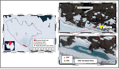
In East Antarctica, Dronning Maud Land’s meteorological and glaciological conditions are characterized by extreme cold, strong winds, and vast ice masses (Horwath et al. 2006). It is a critical area for scientific research, providing insights into climate history and the behavior of the Antarctic Ice Sheet. During the winter months, temperatures can plummet well below −40°C (−40°F), and it can even reach as low as −60°C (−76°F). The region is known for its strong katabatic winds, which are cold, dense air masses that flow downhill from the interior of the continent toward the coast. These winds can reach speeds of over 100 kilometers per hour (62 miles per hour) and significantly influence the local climate (Grazioli et al. 2017). The specific focus of the UAV surveyed area, covering around 100 acres, is a section of the ice sheet frontal edge adjacent to the Maitri, Indian research base at the Schirmacher Oasis (Schirmacheroasen), located inland to central Dronning Maud Land (cDML). The Schirmacher Oasis is a ice-free landscape region spanning 35 square kilometers and situated 100 meters above mean sea level. This area is characterized by a diverse array of lakes, including landlocked, proglacial, and epishelf lakes, and it is positioned between the boundaries of the continental ice sheet and the coastal Nivlisen ice shelf (Warrier et al. 2014). Notably, within the surveyed region, there is a significant feature, a supraglacial lake with coordinates 70° 46’ 22.13” S, 11° 45’ 11.62” E covering an area of 9,500 square meters (Figure 1). This particular lake holds immense importance as it presents an opportunity for targeted research into the dynamics and characteristics of the water body system.

Figure 1. Study area near the Maitri station, cDML, East Antarctica.

3. Dataset overview

To carry out the study, extensive fieldwork was conducted during the austral summer period from November 2022 to February 2023. This included the use of the UAV for aerial surveys, establishing of Ground Control Points (GCPs) using Global Navigation Satellite Systems (GNSS) survey techniques for accurate georeferencing of collected data, and the deployment of pressure sensor assembly (PSA) for melt pond parameters. Having done 19 UAV surveys, only 10 best survey samples covering the study area is considered for the investigation and analysis. Prior to the UAV survey, calibration procedures were performed for the Inertial Measurement Unit (IMU), compass, camera, and other sensors in accordance with the operations handbook. This step was undertaken to ensure accurate and reliable data collection during the UAV survey.

3.1 UAV surveys and flight planning

In the current investigation, aerial surveys were conducted using P4 RTK (real-time kinematic) Multispectral unmanned aerial vehicle (UAV) outfitted with a multispectral camera. A comprehensive UAV data collection effort was undertaken, consisting of a total of 19 surveys between November 25^th, 2022, and January 6^th, 2023. Each survey included three missions, and within each mission, a total of eight flights were executed, resulting in a combined total of 152 flights. In each individual survey, a substantial dataset was obtained, comprising a total of 30,000+ ultra-high-resolution images. However, for subsequent analysis, a discerning approach was applied, and only the top 10 surveys, based on predefined criteria, were selected for further investigation. This ensured that the subset chosen for analysis represented the highest quality and relevance within the dataset. The imaging system consists of six 1/2.9” CMOS sensors, each measuring 2 mega pixels, with one RGB sensor for visible light imaging and five monochrome sensors for multispectral imaging (Figure 2). It also has an inbuilt sunshine/sunlight sensor. The UAV was flown at a height of 95 meters above take-off point, with a view angle of 90 degrees, and ground resolution of 5 centimeters per pixel. In order to provide hover and capture options along with the required overlaps, the UAV’s speed was set at 5 meters per second. In order to interpret UAV data, the survey was designed to obtain a frontal overlap of 75% and a side overlap of 60%.

Figure 2. (a) Multispectral sensor-based UAV used during the aerial survey at East Antarctica (b) field photograph.

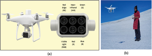
The RTK feature of the UAV employed in this study allows positional accuracy with a multispectral sensor, and it has a net weight of 1,487 grams. The UAV under consideration for the study has a single RGB camera as well as a multispectral camera array with five cameras covering the blue, green, red, red edge, and near-infrared bands (NIR), all of which are 2-megapixel global shutter cameras and are mounted on a 3-axis stabilized gimbal. Additionally, a survey using the global navigation satellite system (SP 80) was conducted to gather nine GCPs outside the ice sheet (over the stable regions, Figure 1).

3.2 UAV & weather data

The present study extensively utilizes ultra high-resolution UAV datasets to obtain detailed and precise information about the study region. Specifically, approximately 10 suitable datasets have been collected and employed for analysis, as outlined in Table 1. These UAV datasets offer a wealth of valuable information, including high-resolution imagery and topographic data for hydrological measurements. To ensure high positional precision and minimize elevation-dependent biases, the GCPs were strategically placed in the field (Figure 3) with printed black and white crosses over stable sections. The GCP survey was conducted using SP80 Spectra Precision GNSS receivers.

Figure 3. Printed black and white crosses.

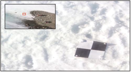
Table 1. Details of UAV mission survey over East Antarctica’s cDML.

Sl No.	Date of UAV survey & data Acquisition	Number of Images
1.	25/11/2022	1,090
2.	30/11/2022	1,005
3.	10/12/2022	1,005
4.	17/12/2022	1,655
5.	18/12/2022	1,605
6.	20/12/2022	2,675
7.	22/12/2022	2,755
8.	24/12/2022	2,690
9.	26/12/2022	2,715
10.	06/01/2023	2,705

For the purpose of analysis, weather information for the study area was obtained from the automatic weather station (AWS) installed 2 m above surface near Maitri station by Indian Meteorological Department (IMD), Government of India. The IMD database provides comprehensive and detailed weather data for Indian Antarctic research bases (Maitri & Bharati). The specific weather data for the study area was accessed through the following link: https://nwp.imd.gov.in/maitri_mausam.php.

3.3 Pressure sensor assembly

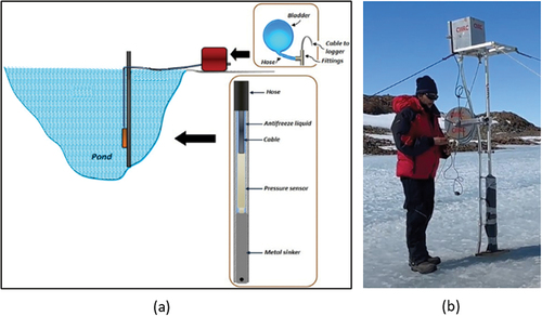
Due to logistical considerations, it was decided to install the Pressure Sensor Assembly (PSA) close to the Maitri, Indian research base in Dronning Maud Land, East Antarctica (11°45’6.786“E, 70°46’22.475“S) during the fieldwork. The current design of the Pressure Sensing Assembly (PSA) is visually represented in Figure 4. To ensure accurate pressure measurements, an armored silicon hose with a diameter of 26 mm and a total length of 10 m was utilized. This hose houses a pressure sensor. The pressure sensor is connected to a slightly larger than 26 mm iron rod, measuring 23 cm in length. The rod is inserted into the hose using silicone sealant and secured with hose clamps in the lower half of the hose. The purpose of the rod is twofold: it acts as a waterproof seal and provides weight to keep the sensor in place. At the top end of the hose, a T-junction is installed to facilitate the connection of the pressure sensor to the data logger via a logger cable. Another branch of the T-junction connects to a 2 L expansion rubber bladder. The bladder is typically filled halfway to accommodate volume changes in the antifreeze solution, such as those caused by solar heating, without generating excess pressure within the assembly. The hose itself is filled with a 50:50 mixture of ethylene glycol and water, serving as the antifreeze solution. To mount the PSA, a 5 m-long pole is erected in the middle of the supraglacial lake area. The PSA is attached to the pole using a Teflon pulley and guides. This pulley arrangement ensures that the pressure sensor descends as the ice melts, maintaining contact with the bottom surface of the pond or lake where meltwater accumulates. The installation process involves drilling into the frozen pond using a Jiffy ice auger (4 G four stroke) and extenders, reaching depths of up to 3 m. This setup was completed by late November 2022, well before the melting period.

Figure 4. (a) Graphical design and actual installation of the Pressure Sensor Assembly over the melt pond; (b) PSA setup over the melt.

3.4 Pressure sensor DCX-22

The pressure sensor utilized in the PSA is the DCX-22 data logger from KELLER Druckmesstechnik AG, Switzerland, known for its versatility in measuring water level, water pressure, and temperature. The specific variant used is the Sealed Gauge, which offers the highest level of accuracy (±2. 5 cm) and is suitable for submersion applications. With an extended battery life, the DCX-22 data logger can record data for up to 10 years, capturing measurements at hourly intervals. The user has the ability to calibrate the pressure sensors integrated within the DCX logger unit. The calibration process is carried out using the KOLIBRI Desktop program. It is crucial to ensure that the sensors are examined or calibrated in the same positions they occupy at the measuring point, typically in an upright position. Furthermore, the sensors should be placed adjacent to each other at the same level. There are various situations where these sensors may require recalibration, such as during maintenance activities, when altering the measurement configuration, or after the measuring station has been operational for a year or more.

3.5 PSA data collection

The pressure sensor, in conjunction with the data logger, was programmed to gather both pressure and temperature data at regular intervals of every 15 minutes. This configuration ensured that precise measurements were captured throughout the monitoring period. To prevent data loss due to low battery or memory issues and to maintain continuous contact between the sensor and the melt pond ice floor or bottom bed surface, the data was retrieved from the logger on a daily basis manually. However, it is important to note that certain data gaps were encountered when the sensor became exposed due to the freezing of the pond or reduced water levels after late December 2022. These factors interrupted the data collection process during those periods. Within the context of this study, the supraglacial lake depth was precisely defined as the vertical separation between the water level and the lowest point of the melt pond or SGL bed within the specific cross-section under investigation. This definition allows for a comprehensive understanding of the depth of the melt pond or SGL, taking into account variations in topography and the underlying bed surface. Figure 5 illustrates the mean temperature and hydrostatic pressure values recorded by the sensor at the bottom of the melt pond throughout the fieldwork period. These measurements provide valuable insights into the thermal and hydrological characteristics of the melt pond. When it comes to determining the height of the water column using the hydrostatic pressure measured by the DCX-22 device, it is essential to consider the density of the medium. The KOLIBRI Desktop software, employs Equation 1(1) $d=\frac{P}{\rho \ast g}$(1) to calculate the water column height. This equation allows for the conversion of pressure readings in N/m² to the corresponding height of the water column in meters. The calculation takes into account a water density of 999.89 kg/m³, which is based on the average temperature observed on December 20^th, 2022, at around 1°C. Additionally, the length of the iron rod has been factored into the depth estimates to ensure accurate measurements.

Figure 5. The pressure sensor assembly installed was monitored for 25 days during the Austral summer of 2022–2023 to determine the hydrostatic pressure and temperature.

(1) $d=\frac{P}{\rho \ast g}$(1)

where p = hydrostatic pressure (N/m²), ρ = water density (kg/m³), g = gravitational acceleration (m/s²), d = height of water column (m)

3.6 Ground validation points (GVPs)

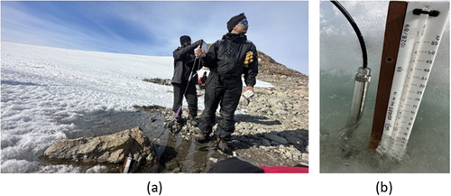
To gather additional data and validate the measurements obtained from the PSA system, manual measurements of the melt pond’s depth and temperature were conducted at various locations distributed around the perimeter of the pond (Figure 6). These manual measurements served as ground validation points (GVPs) and provided supplementary information to cross-check and validate the accuracy of the PSA system’s measurements. However, in the interior of the melt pond, where manual interventions were not feasible due to the evolving melt process, including the presence of slush and large melt channels, the PSA system played a crucial role in measuring the depth. Designed specifically for this purpose, the PSA system was able to overcome the challenges associated with manual measurements in such conditions. To ensure accuracy and consistency, both the PSA installation point and the locations of the manual measurement points were surveyed as ground validation points. This surveying process further enhanced the reliability of the data collected and allowed for comprehensive analysis and comparison between the PSA measurements and the manual measurements taken at specific points within the melt pond.

Figure 6. (a) Manual depth measurements (b) pressure sensor with the thermo sensor.

4. Methodological framework

4.1 UAV data preprocessing

Agisoft Metashape Professional Edition 2.0.1 is a powerful software used for processing UAV images. It performs a range of functions to transform the raw UAV images into valuable geospatial data. The UAV data processing steps were adopted from “Agisoft Metashape User Manual: Professional Edition, Version 1.8” and parameters related to align photos accuracy, cloud point quality, and DEM quality were set to high. The first step in the process is image pre-processing, which includes tasks such as image alignment, calibration, and distortion correction to prepare the images for further analysis. The process of Structure-from-Motion (SfM) is utilized in photogrammetry to create a three-dimensional representation of a scene by analyzing a set of overlapping images. This feature extraction is conducted, where the software identifies and matches key features across multiple images to ensure accurate alignment and reconstruction. This step enables the generation of a dense point cloud, utilizing photogrammetric techniques that reconstruct the 3D coordinates of objects and surfaces captured in the UAV images. The dense point cloud data is then used to generate a DEM, providing elevation information for the surveyed area, and high-resolution orthophotos (Themistocleous 2019). These orthophotos are georeferenced and corrected for perspective distortions, ensuring their suitability for subsequent analysis. To achieve precise georeferencing, the software incorporates GPS data and GCPs. GCPs serve as reference points with known coordinates, allowing for precise alignment of the processed images with real-world coordinates. The Ground control points (GCPs) and checkpoints play a vital role in UAV surveys to ensure the accuracy and georeferencing of the collected data. They contribute to the reliability of survey results, and facilitate quality control. In general, for small to medium-sized surveys, 3–5 GCPs along with 3 or more checkpoints are used to validate the survey’s accuracy. Additionally, the use of RTK-enabled UAVs can reduce the required number of GCP (Masný, Weis, and Biskupič 2021). By using the information in the log files during post-processing, adjustments can be made to improve the overall accuracy of the survey results. This may involve refining the drone’s positional data based on the detailed information logged during the flight (Karušs et al. 2022; Lamsters et al. 2022)

4.2 UAV data post processing

The utilization of the surveyed datasets in the study of melt pond dynamics was conducted on a total of 10 datasets. All post processing were carried out in Quantum GIS software. However, when it came to investigating mass balance and cryofacies studies, only four datasets were employed. This discrepancy arises from the fact that these four surveys possessed two distinct advantages: they encompassed uniformly surveyed areas and exhibited larger coverage compared to the other datasets. The UAV data preprocessing and post processing are shown in Figures 7 and 8 respectively.

Figure 7. Agisoft metashape process flow.

Figure 8. Process flow adopted for estimating (a) ice sheet front/edge mass balance – M1 (b) &; (c)Melt Pond dynamics – M2 & M3 (d) cryofacies – M4 and (e) in-situ measurements – M5.

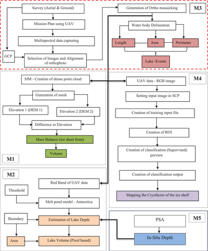
Regarding the mass balance analysis, six combinations of differenced elevations were derived from the four generated Digital Elevation Models (DEMs). These combinations were computed to capture the changes in elevation over time and provide insights into the mass balance dynamics of the surveyed regions. The differenced elevation values enable researchers to examine variations in ice thickness change, snow accumulation, and meltwater runoff, which are crucial factors in understanding the overall mass balance of the studied area. The elevation differences were used to calculate the mass balance of the ice sheet margin over a 7-day interval, utilizing Equation 2(2) $V=A_e\ast T_a$(2) -Equation 5(5) $M^{\prime }=\frac{M}{{\to }^{\prime }}$(5) .

(2) $V=A_e\ast T_a$(2)

(3) $m=\to \ast V$(3)

(4) $M=\frac{m}{T_a}$(4)

(5) $M^{\prime }=\frac{M}{{\to }^{\prime }}$(5)

where, V is the volume, A_e is the change in elevation, T_a is the total area, m is the mass, → is the density of ice, M is the mass per unit area, $M^{\prime }$ is the mass balance in m.w.e, →^’ is the density of water.

In the context of cryofacies analysis, a supervised classification technique was applied to an RGB image (Raghavendra, Geetha Priya, and Sivaranjani 2023). Beforehand, the classification model was trained using sample datasets, allowing it to learn and distinguish different cryofacies classes. The RGB image served as the input, and the trained model classified each pixel into specific cryofacies categories based on its spectral characteristics. A supervised pixel-based (Maximum Likelihood) classification technique with appropriate training samples was employed. A total of 600 training pixels were used, with around 100 pixels trained for each class. The UAV images were classified into different classes including water body/meltwater, frozen water, bedrock, debris/bare ice, and wet/dry snow.

To evaluate the melt pond characteristics, a manual delineation process was conducted on the RGB image. We visually outlined the boundaries of melt ponds and extracted relevant parameters, including area, length, and shape. By comparing these parameters obtained from Unmanned Aerial Vehicle (UAV) data, we were able to identify and analyze events related to the formation/melting, draining, and refreezing of the melt pond. These findings contribute to a deeper understanding of the temporal evolution and dynamics of melt ponds within the studied areas (Lindbäck et al. 2019).

To estimate the depth of the supraglacial lake, a melt pond depth model given in equation 6 has been used. The model utilizes red band data and is based on the radiative transfer concept (Arthur et al. 2020), which simulates the interaction of light with various components of the lake environment. By considering factors such as light attenuation, water absorption and scattering properties, and lake bottom albedo, the model calculates the depth of the water column and the calculated depth is used to determine the volume of the supraglacial lake (Land et al. 2023).

(6) $L_d=\frac{\left[ln\left(L_{br}-R_{\mathrm{\infty }}\right)-\mathrm{l}\mathrm{n}\left(R_{Ld}-R_{\mathrm{\infty }}\right)\right]}{\alpha }$(6)

Where, $L_{br}$ is peripherals reflectance of the lake, $R_{\mathrm{\infty }}$ is the reflectance of optically deep water, $R_{Ld}$ is the reflectance of the water body, $\alpha$ is the attenuation constant. By averaging two pixels buffer, the L_br was derived for the melt pond in each scene and $R_{\mathrm{\infty }}$ value was assumed to be 0 (Arthur et al. 2020; Geetha Priya et al. 2022; Pope et al. 2016).

5. Results

5.1. DEM & mass balance

The Digital Elevation Models (DEMs) obtained from UAV-captured raw images possess a spatial resolution of 8.5 cm. These DEMs covered areas ranging from 0.268 km² to 0.278 km². By overlapping these DEMs, a common region containing the frontal edge of the ice sheet was selected for the mass balance study. This specific region was chosen due to its observed high rate of mass change. The root mean square error (RMSE) of 2.4 cm was calculated by comparing elevations of over 100 points in stable regions between two DEMs using Equation 8(8) $U=\hspace{0.17em}\sqrt{u_{meas}^2+u_{spatial}^2+u_{temporal}^2+u_{model}^2+u_{analysis}^2}$(8) .

(7) $RMSE=\sqrt{{\sum }_{i=1}^N\frac{{(x_i-\hspace{0.17em}{x}_i^{\prime })}^2}{N}}\hspace{0.17em}$(7)

Where N is the number of points considered, $x_i$ is the elevation value of the DEM1 and $x{ }_i^{\prime }$is the elevation of the DEM2. The two DEMs were aligned and registered for DEM differencing using image to image co-registration plugin in QGIS. To eliminate outliers, elevation changes exceeding 4.5 meters and below −2.5 meters in the differenced DEM were identified and removed. These extreme elevation changes typically occur at the edges of the DEM. Additionally, pixels exhibiting an absolute elevation difference greater than three standard deviations from the mean were excluded. This process, combined with the earlier mentioned outlier threshold, effectively eliminated anomalous data points from the analysis.

The analyzed ice sheet frontal edge margin area, after the removal of outliers and non-overlapping regions, approximately spans 59,384 m². For December 2022, a series of four Digital Elevation Models (DEMs) were generated for the dates: the 20^th, 22^nd, 24^th, and 26^th. To accurately assess the mass balance, six combinations of elevation differences were calculated based on these DEMs. Table 2 presents the mass balance results that includes mass gain and loss (three density scenarios of exposed firn 840 kgm⁻³, ice 900 kgm-3 and melting ice 960 kgm⁻³ are considered for error calculation) (Farías-Barahona et al. 2020). Figure 9 displays the minimum, maximum, and average elevation differences observed. To gain insights into the mass change rate, the mass balance was estimated for different intervals within the same week. It was observed that over a two-day interval (from the 20^th to the 22^nd of December 2022), there was an average elevation gain of 0.28 m and a mass gain of 15.34 kilotons. Furthermore, during a four-day interval (from the 20^th to the 24^th of December 2022), it was observed approximately 40 kilotons of mass was accumulated with an average elevation gain of 0.75 m. Conversely, there was a mass loss of 24.64 kilotons and an average elevation loss of 0.46 m within a two-day interval (from the 22^nd to the 24^th of December 2022). Another observation was made during a four-day interval (from the 22^nd to the 26^th of December 2022), where 29 kilotons of mass was lost with an average elevation loss of 0.54 m. Finally, a significant mass gain of 53.68 kilotons and an elevation gain of 1 m were observed within a two-day interval (from the 24^th to the 26^th of December 2022).

Figure 9. Minimum, maximum and average elevation changes of the ice sheet frontal edge margin.

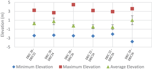
Table 2. Mass balance for an ice density of 900 ± 60 kgm⁻³ during December 2022.

Dates	Mass Balance (m.w.e)	Mass Balance (Kt)
DEC20-DEC22	0.25±0.01	15.34±1.02
DEC20-DEC24	0.67±0.04	39.95±2.60
DEC20-DEC26	−0.23±0.01	−13.60±0.90
DEC22-DEC24	−0.41±0.02	−24.64±1.64
DEC22-DEC26	−0.48±0.03	−29.00±1.93
DEC24-DEC26	0.90±0.06	53.68±3.57

5.2. Image re-projection and XYZ errors

The UAV image reprojection error refers to the discrepancy between the projected positions of points in an unmanned aerial vehicle (UAV) image and their corresponding ground truth positions. These errors represent the level of accuracy or precision in the spatial positioning of the collected data. The reprojection error for the surveys was measured in the range of 0.1–0.15 pixels. During the process of georeferencing and orthorectification, the positions of ground control points (GCPs) are used to establish the transformation model. However, due to various factors such as sensor errors, lens distortion, atmospheric conditions, and inaccuracies in GCP measurements, there can be errors in the reprojection of the UAV image.

UAV images are utilized to create dense point clouds, which serve as a comprehensive three-dimensional depiction of the object or scene (Weiss and Baret 2017). The dense point cloud comprises a multitude of data points, with each point representing a distinct spatial location. Furthermore, each point within the dense point cloud contains valuable information about its specific X, Y, and Z coordinates (in this context, the X coordinate denotes longitude, the Y coordinate corresponds to latitude, and the Z coordinate signifies altitude). The observed horizontal (XY) and vertical (Z) errors were found to be 1–1.2 cm and 1.1 cm, respectively. In the context of UAV data or point cloud data, XYZ errors typically refer to the differences between the measured or derived coordinates of points in the point cloud and their corresponding ground truth or reference coordinates. These errors can arise from various factors such as sensor inaccuracies, positioning errors, calibration issues, atmospheric conditions, or limitations in the measurement or processing techniques.

5.3 Dynamics of the melt pond

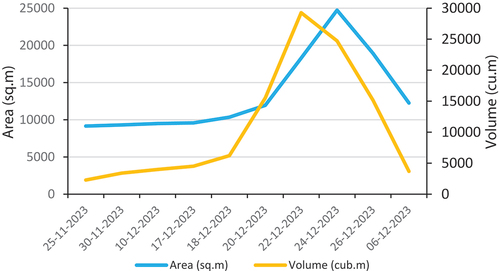
Melt Pond statistics were collected through 10 surveys conducted using Unmanned Aerial Vehicles (UAVs) between November 25^th, 2022, and January 6^th, 2023. These surveys provided valuable information about the characteristics and dynamics of the melt pond during this period. Examining the average depth of the melt pond reveals fluctuations between 0.25 meters and 1.60 meters. This indicates changes in the water depth within the pond over the observed period. Factors such as temperature variations, precipitation, albedo, katabatic wind and drainage could contribute to these fluctuations. The length of the melt pond increased from 290 meters to 541 meters (Figure 10) during the surveyed timeframe linked to increased melt water accumulation or the merging of smaller melt ponds. One notable trend observed in the data is the increasing volume of the melt pond. Starting from 25 November 2022, the volume recorded was 2,279 cubic meters, and it steadily increased over time, reaching its highest value of 29,272 cubic meters on December 24^th, 2022 (Figure 11). The perimeter of the melt pond also displayed a general increasing trend, starting at 658 meters and reaching a maximum of 1,184 meters with the area of the melt pond varying from 9,151 square meters to 24,727 square meters. This indicates that the melt pond accumulated more melt water as the season progressed, likely due to melting ice. The increase in area aligns with the observed trends in volume and perimeter. However, after December 24^th, 2022, the pond parameters (depth, area, volume, perimeter and length) started to decrease, likely due to refreezing, snowfall, reduced melting, and potential drainage through internal cracks, fractures, channels or other pathways. Section 3.5 discusses about the in-situ measurements of the water depth measured using PSA.

Figure 10. The perimeter, length and depth profile of the melt pond for the surveyed dates.

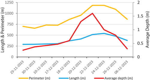
Figure 11. The area and volume profile of the melt pond for the surveyed dates.

5.4 Cryofacies

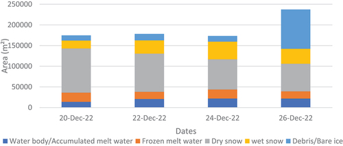
UAV data collected between December 20^th, 2022, and December 26^th, 2022, were utilized for cryo-facies mapping. The UAV images were classified into different classes including water body/meltwater, frozen water, bedrock, debris/bare ice, and wet/dry snow. The results of the cryo-facies mapping are presented in Figures 12 and 13. The area of water bodies or accumulated meltwater on December 20^th, 2022, was 13,895 m², which increased to 21,830 m² on December 22^nd, 2022. There was a slight rise to 21,894 m² on December 24^th, 2022, followed by a decrease to 21,691 m² on December 26^th, 2022. This indicates a temporary increase in meltwater accumulation, which gradually declined over the observed period. The area of frozen meltwater was 22,133 m² on December 20^th, 2022, which decreased to 17,155 m² on December 22^nd, 2022. There was a significant increase to 21,675 m² on December 24^th, 2022, followed by a decrease to 17,473 m² on December 26^th, 2022. The decrease in accumulated meltwater and frozen meltwater area during the peak melt season is attributed to drainage through internal fissures, fractures, and channels. The dry snow consistently covered the largest area and there was a gradual decrease in the area of dry snow from 106,864 m² on December 20^th, 2022, to 66,823 m² on December 26^th, 2022. Wet snow exhibited fluctuations, with an increase from 19,324 m² on December 20^th, 2022, to 42,765 m² on December 24^th, 2022, followed by a decrease to 36,293 m² on December 26^th, 2022. The area covered by debris/bare ice experienced significant fluctuations throughout the observed period. It increased from 12,558 m² on December 20^th, 2022, to 15,645 m² on December 22^nd, 2022 and then decreased to 13,704 m² on December 24^th, 2022. However, there was a substantial increase to 95,219 m² on December 26^th, 2022. The area covered by the bedrock remained relatively stable during the observed period. Minor fluctuations were observed, with an increase from 91,530 m² on December 20^th, 2022, to 98,299 m² on December 22^nd, 2022. The area then decreased to 96,910 m² on December 24^th, 2022, and further decreased to 30,529 m² on December 26^th, 2022.

Figure 12. Supervised pixel-based classification cryofacies for the dates December 20^th, 2022, December 22^nd, 2022, December 24^th, 2022, December 26^th, 2022.

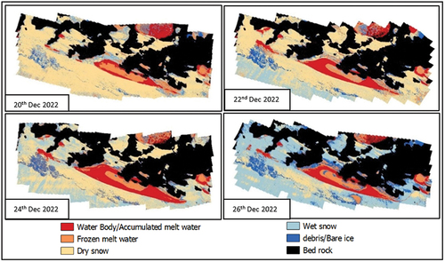
Figure 13. Classification type and the area covered during the supervised pixel-based classification.

5.5 In-situ measurements

In this study, the depth of the melt pond was estimated using multispectral data acquired from an Unmanned Aerial Vehicle (UAV) and the radiative transfer model. The accuracy and reliability of the model-based estimations were evaluated by comparing them with metrics obtained from the Pressure Sensing Assembly (PSA) and manual measurements. Table 3 summarizes this comparison, indicating the root-mean-square error (RMSE) as a measure of the differences between the model-based estimation and the physical in-situ measurements taken at various field locations. It is important to consider uncertainties and time differences between measurements and aerial surveys conducted at different intervals during the observation day, as these factors can introduce variations in the measured depths of the melt pond. Figure 14 presents the regression analysis used to compare the field-based depth measurements with the model-based results along with the field photograph. The plot demonstrates a significant positive linear association between the two datasets, supported by a Pearson’s correlation coefficient of 0.9. This strong correlation coefficient indicates a robust relationship between the field measurements and the estimations derived from the radiative transfer model, providing further evidence of the model’s validity. The utilization of multispectral data and the radiative transfer model proves to be a promising approach for estimating melt pond depth. The results show a strong agreement between the model-based estimations and the in-situ measurements collected in the field, highlighting the effectiveness of this methodology for studying and understanding melt pond dynamics.

Figure 14. On December 22^nd, 2022 (a) correlation analysis of the measured values; (b) the model-based melt pond depth derived from the UAV survey; (c) melt pond view.

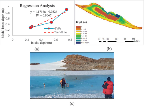
Table 3. The melt pond depth values for 22 December 2022, as determined by the pressure sensor and melt pond depth model.

Parameters	Findings
Validation date of UAV survey data	22^nd December 2022
Depth at GVP (Model-based)	2.04 ± 0.2m
Depth at GVP (PSA-based)	2.19 ± 0.03 m
RMSE	0.15

5.6 Analysis of air temperature and PSA temperature

The temperature measurements obtained from the Pressure Sensing Assembly (PSA) were cross-corroborated with standard devices approved by the World Meteorological Organization (WMO) and carried by scientists from the Indian Meteorological Department (IMD) during the field season. This validation process ensured the accuracy and reliability of the temperature data collected by the PSA. By comparing the measurements from the PSA with those obtained from the standard devices, the study ensures the consistency and quality of the temperature data. This cross-corroboration helps to validate the PSA’s performance in accurately capturing temperature variations in the melt pond environment. The use of WMO-approved standard devices adds an additional level of credibility to the data, as these devices adhere to internationally recognized standards for temperature measurement.

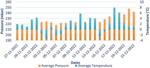
The average air temperature obtained from AWS installed near Maitri and the average surface temperature of melt pond bottom obtained from PSA during December 2022 are analyzed in Figure 15. The average air temperature varied throughout the month, ranging from −4.4°C to 1.8°C. The temperatures showed some fluctuations over the course of the month, with both positive and negative values. However, the overall trend suggests that the temperatures remained relatively low, indicating a cold weather pattern during this period. The average melt pond bottom surface temperatures also exhibited variations during December 2022, ranging from −3.4°C to 8.0°C. It is important to note that the melt pond bottom surface temperatures can be influenced by various factors, including solar radiation, air temperature, and water circulation within the pond. The data shows a mix of positive and negative values, indicating fluctuations in the thermal conditions of the melt pond. Higher temperatures are observed in certain instances, which could be attributed to factors such as solar radiation, atmospheric heat transfer, geothermal heat, subglacial discharge or other localized heat sources.

Figure 15. The average surface temperature of melt pond bottom obtained from PSA during December 2022 and average air temperature from AWS at 2m height near Maitri station.

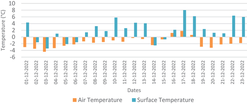
There appears to be a correlation between the average air temperature and the melt pond bottom surface temperature, although the relationship is not strictly linear. In some cases, higher air temperatures coincide with higher melt pond bottom surface temperatures, suggesting a positive relationship. However, there are instances where the air temperature is low, but the melt pond bottom surface temperature remains relatively high (Thielke et al. 2023). This could be due to factors such as insulation effects, heat transfer processes, or localized heat sources within the pond. The observed temperatures during December 2022 provide insights into the thermal conditions of the melt pond. The presence of positive melt pond bottom surface temperatures suggests that there were areas of active melting within the pond, possibly due to solar radiation or geothermal heat sources. The fluctuations in temperatures indicate dynamic thermal processes within the pond, which can influence its overall stability, water circulation, and interactions with the surrounding ice sheet or glacier. It is important to note that this analysis is based on the data that is available during December 2022. Further investigations and analyses, considering additional factors such as solar radiation, wind patterns, and water flow dynamics, would provide a more comprehensive understanding of the melt pond behavior and its implications for the larger glacial system.

6. Discussion

Within the limited timeframe of our brief analysis, distinct periods of positive and negative mass balance were identified over a one-week span, focusing solely on a segment of the ice sheet frontal edge margin. From December 20^th to 26 December 2022, our observations revealed an average elevation decrease of 0.25 meters and a mass loss of 13.6 kilotons during this interval. Positive mass balance, as indicated by the gaining of ice at the ice sheet edge through processes like snowfall or glacier flow, contrasts with the losses incurred through melting, calving (iceberg detachment), and sublimation (Kapsch et al. 2021; Smith et al. 2020). Analysis of Figure 16 revealed an absence of precipitation during the study period, signifying ice sheet movement toward the margin. This movement coincided with a reduction in average temperatures, ranging from −3.2°C on 20 December 2022, to −0.5°C to −4.4°C on December 24 and 26, 2022. Glaciers and ice sheets exhibit accelerated flow or movement near their margins due to gravity-induced downhill flow, with higher shearing stress at the edges compared to the center (Benn, Evans, and Holloway 2010; Chandler and Evans 2021). Negative mass balance, observed from December 20 to 26, 2022, denotes the condition where the ice sheet edge loses more ice than it gains, potentially resulting in the retreat or thinning of the ice sheet edge and overall ice sheet shrinkage. Contributing factors include increased melting, elevated average temperatures, albedo effects, katabatic winds with enhanced calving rates, or reduced snowfall (Lenaerts et al. 2019; Liu et al. 2015; Trusel, Kromer, and Datta 2023). The intricacies of ice sheet mass balance remain an active area of research, demanding a multidisciplinary approach involving satellite observations, field measurements, and numerical modeling (Lenaerts et al. 2019). Surface mass balance (SMB) serves as a crucial factor in determining mass input to the Antarctic and Greenland Ice Sheets, exerting control over ice sheet mass balance and contributing to global sea level changes (Noble et al. 2020). The SMB’s complexity, varying across multiple spatial and temporal scales, poses challenges in observation and representation within models. It comprises multiple components, with dependencies on intricate interactions between the atmosphere and the snow/ice surface, large-scale atmospheric circulation, and ice sheet topography (Bindschadler, Clark, and Holland 2010).

Figure 16. Average temperature and precipitation data from AWS installed by IMD located near Maitri research base.

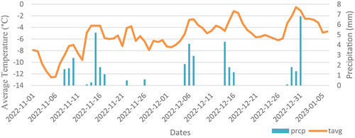
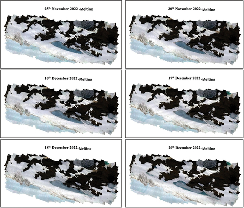
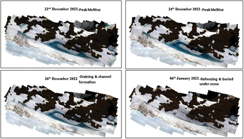
The temperature fluctuations observed during the study period are likely to have played a crucial role in the dynamic interplay of melting and freezing processes within the supraglacial lake. This interaction is further influenced by albedo and katabatic wind-driven feedbacks, as highlighted in previous studies (Arthur et al. 2020; Kingslake et al. 2017). The daily average air temperature ranged from −6.2 degrees Celsius to −4.7 degrees Celsius, with the maximum air temperature fluctuating between −4.2 degrees Celsius and 0.3 degrees Celsius. In East Antarctica, katabatic winds are characterized by strong easterly winds descending with speeds of up to 19 meters per second, driven by steep surface gradients exceeding 20 degrees (Doran et al. 1996). As these winds descend toward the grounding zone, adiabatic warming occurs, leading to reduced humidity and higher near-surface air temperatures (Doran et al. 1996; Lenaerts et al. 2019). The presence of blue-ice areas, with a lower albedo of approximately 0.5 compared to refrozen snow at around 0.7, contributes to a positive feedback mechanism by enhancing the absorption of solar radiation (Kingslake et al. 2017; Lenaerts et al. 2019; Stokes et al. 2019). This albedo-reducing feedback loop is notably intensified in the study area and nearby nunataks, resulting in increased surface melting and pond formation. The temperature-dependent processes observed include melting, peak melting, channel formation and draining, and eventual freezing and burial under snow, as illustrated in Figure 17. Higher temperatures promote melting, whereas lower temperatures facilitate freezing and the potential formation of ice layers over the lake (Lampkin et al. 2020; Maier et al. 2023). The intricate sequence of events witnessed on the melt pond throughout the surveyed period underscores the complex interplay of climatic factors influencing supraglacial lake dynamics in the East Antarctic region.

Figure 17. Melt pond events captured during the UAV survey.

The examination of classified cryofacies data presents valuable insights into the intricate dynamics of the observed region between December 20th and 26 December 2022. A noteworthy observation during the peak melt season is the reduction in both accumulated meltwater and frozen meltwater areas. This phenomenon is primarily ascribed to drainage mechanisms operating through internal fissures, fractures, and channels within the ice sheet, as discussed by French, and Shur (2010) and Stephani et al. (2010). It is crucial to acknowledge that these fluctuations are not exclusively driven by drainage processes; rather, they are likely influenced by temperature variations and local conditions, emphasizing the multifaceted nature of meltwater behavior. The gradual decrease in dry snow coverage over the same period suggests an ongoing process of snowmelt or redistribution, potentially driven by evolving environmental conditions. The variations in the amount of wet snow can be attributed to changing temperatures and precipitation patterns, underscoring the sensitivity of snow types to meteorological factors. Furthermore, the observed changes in the exposure of bare ice and debris indicate dynamic processes such as snow and ice melting or the deposition of debris. Lastly, fluctuations in the exposure of bedrock may result from a combination of factors, including ice melt and the freezing of meltwater. In summary, this analysis highlights the natural processes within the cryosphere and their sensitivity to climate and environmental changes. The observed dynamics contribute to our understanding of broader glaciological processes, showcasing the complex relationships among temperature variations, precipitation patterns, and internal ice sheet structures.

6.1 Limitations and uncertainties

The primary focus of this study was the analysis of the supraglacial lake and the ice sheet frontal edge margin in the vicinity of Maitri station. These features exhibit significant temporal and spatial variability. The specific time period under investigation spanned from November 25^th, 2022, to January 06^th, 2023, during which the estimation of melt pond features, cryofacies mapping, and ice sheet margin mass balance was conducted. It should be noted that certain factors with the potential to impact water level changes were not considered in this study. These factors include the occurrence of large or small debris slumps, ice calving events, the influence of katabatic winds, pond floor collapse, subaqueous melting, structural instability, and variations in water storage resulting from the interplay between water filling (melting) and drainage (discharge). The omission of these factors in the analysis limits our understanding of the full range of influences on water level fluctuations and their environmental implications. Due to practical constraints, the installation of measurement equipment was carried out at a single designated location within the melt pond. Consequently, the validation of melt pond depth estimations was performed using data obtained from the Pressure Sensing Assembly (PSA), allowing for the assessment of both model-based predictions and manual measurements.

Although limited to a single location, this setup facilitated the evaluation and validation of the estimated melt pond depths, providing valuable insights into the accuracy and reliability of the model-based and manual estimations. As the UAV data post processing was conducted through QGIS, the absence of metrics hinders the assessment of the approaches used.

In our UAV survey, we utilized nine ground control points (GCPs) to obtain accurate and georeferenced data. However, we did not use any checkpoints to validate the accuracy of the survey. While checkpoints are not mandatory for data processing, they are useful for post-processing verification of map accuracy. The use of checkpoints can help ensure that the survey results are reliable and adhere to industry standards and regulations. To address this limitation, future survey methodologies will incorporate checkpoints to fortify the accuracy validation protocol. In general, it is recommended to use three or more checkpoints to validate the accuracy of the survey. However, the specific number of GCPs and checkpoints required can vary depending on the project’s accuracy requirements and the specific conditions of the survey area (Karušs et al. 2022; Lamsters et al. 2022; Masný, Weis, and Biskupič 2021).

Figure 17. (Continued).

In this study, several sources of uncertainty need to be considered. Measurement errors may arise due to inherent inaccuracies or errors associated with the measurement devices used, including sensors, instruments, and data loggers. The spatial variability of melt pond characteristics and ice sheet margin conditions introduces uncertainty as measurements taken at different locations within the study area may exhibit variations. Similarly, the temporal variability of these features, influenced by weather conditions, melting processes, and other dynamic factors, adds uncertainty to capturing the complete dynamics within the limited study time frame. The model-based estimations of melt pond depth may be subject to uncertainties resulting from the assumptions and simplifications made in the radiative transfer model (Popović and Abbot 2017). Furthermore, uncertainties can arise during data processing and analysis, including calibration procedures, interpolation methods, and statistical analyses employed, which can affect the accuracy and reliability of the results. It is crucial to acknowledge these uncertainties to provide a comprehensive understanding of the study’s limitations and potential sources of error. By quantifying and accounting for these individual sources of uncertainty, the equation 8 provides an estimation of the overall uncertainty of 2% to 5% in the study’s findings and results.

(8) $U=\hspace{0.17em}\sqrt{u_{meas}^2+u_{spatial}^2+u_{temporal}^2+u_{model}^2+u_{analysis}^2}$(8)

Where, U represents the overall uncertainty in the study, $u_{meas}$ represents the uncertainty associated with measurement errors, $u_{spatial}$ represents the uncertainty arising from spatial variability, $u_{temporal}$represents the uncertainty due to temporal variability, $u_{model}$ represents the uncertainty associated with the model-based estimations, and $u_{analysis}$ represents the uncertainty related to data processing and analysis techniques. The estimation of uncertainty can vary significantly depending on the individual quantity, the type of data or measurements involved, and the standards or best practices relevant to that field.

6.2 Challenges and observations in UAV surveys in Antarctica

Unmanned Aerial Vehicles (UAVs) are increasingly being used in Antarctic environmental research due to their practicality, rapid data collection, and precision (Cassano et al. 2021). However, their use in this region comes with several challenges. The demanding Antarctic conditions, including severe weather, restricted flight time during the austral summer season, and inaccessibility to study areas, make comprehensive data collection and multidisciplinary research difficult (Krause et al. 2021). The harsh environment of Antarctica poses operational problems for UAV surveys. Extreme weather conditions, limited flight time, and inaccessibility to study areas hinder data collection and impede the progress of research (Li et al. 2023). Despite these challenges, UAVs have been shown to be effective tools for environmental and wildlife research in Antarctica.

For the present study, each survey over the study region required five overlapping flight missions on suitable weather days, with wind speeds ranging from 4 to 7 meters per second (m/s). These flights drained the 90Wh batteries of the UAVs completely due to the sub-zero temperatures. Each survey resulted in capturing over 2000–2750 images. However, not all aerial surveys yielded successful data capture, as only 10 out of the 19 surveys conducted during the 42nd ISEA provided good samples over the study area. Similar challenges were encountered during the UAV surveys conducted during the Indian Arctic Expedition-2019 by the team members (Geetha Priya et al. 2022). These challenges stem from the severe climate conditions in Antarctica, the Arctic, and the Himalayas, which require expertise and sound knowledge in UAV handling and operations (Bello et al. 2022). The presence of compass/magnetometer anomalies near the poles also greatly impacts UAV flights and can result in crash landings (Pina and Vieira 2022). The negative temperatures and strong katabatic winds, which increase with flying elevation, pose risks to the UAV’s battery performance and flight time. In extremely cold weather, the battery drains faster, and the UAV becomes more susceptible to destabilization by wind gusts (Tovar-Sánchez et al. 2021). To overcome these challenges, adjustments in flight altitude were necessary to achieve the required ground resolution, although this led to a trade-off between the area covered and the resolution, making it difficult to obtain high-quality data.

Several key learnings and observations were made during the 42nd ISEA UAV surveys:

• Images captured using “capture mode” take images along the flight path on the fly, which doesn’t provide required overlaps in forward and sideward directions. Images without frontal overlap of 75% and side overlap of 60% are not suitable for generating useful orthoimages and DEM. Also often affects sensor stability.

• Flying in hover and capture mode, where the UAV stops for each image, yields the required overlaps and sensor stability but is time-consuming and drains the battery faster.

• The surveying time was limited and insufficient to complete all flight missions, including IMU calibration, compass calibration, sensor calibration, mission planning and waypoint definition, Ground Control Point (GCP) survey, and flying in hover and capture mode due to harsh weather.

• Sudden strong gusts of wind during UAV flights can pose risks, and in such situations, the flight is temporarily suspended until the wind subsides.

7. Conclusion

The study demonstrates the value of utilizing state-of-the-art multispectral sensor-equipped UAV for comprehensive cryosphere research in challenging environment East Antarctica’s Dronning Maud Land region during austral summer 2022–2023. The proposed work is the first of its kind to the best of our knowledge that contains time series of ultra-high resolution UAV data with shortest temporal resolution possible to uncover the changes in mass balance of a segment of ice sheet frontal edge margin along with cryofacies features and melt pond dynamics with in-situ measurements. The observed fluctuations in meltwater accumulation, frozen meltwater, snow cover, and the behaviors of supraglacial lakes reflect the sensitivity of these systems to various environmental factors, including local weather, albedo & katabatic wind feedbacks and drainage processes through internal pathways. This study provides a better understanding of ice sheet dynamics and lake events in short duration by filling the knowledge gaps contributing to our broader understanding of the cryosphere and its response to changing climate conditions in the East Antarctic region.

Acknowledgments

The authors acknowledge the logistical support given by the National Centre for Polar and Ocean Research, Ministry of Earth Sciences, Govt. of India under the Indian Scientific Expedition to Antarctica (ISEA) with project code 42-AMOS/OR-06(2) to undertake this research. The authors gratefully acknowledge the support rendered by PTICL, MM Forgings, TATA STEEL, Jyothy Industries, Rational Technologies and CIIRC, Jyothy Institute of Technology, Bengaluru.

Disclosure statement

The authors declare that they have no known competing financial interests or personal relationships that could have appeared to influence the work reported in this paper.

Data availability statement

Data will be made available on request.

Correction Statement

This article has been republished with minor changes. These changes do not impact the academic content of the article.

References

- Ahmed, F., J. C. Mohanta, A. Keshari, and P. S. Yadav. 2022. “Recent Advances in Unmanned Aerial Vehicles: A Review.” Arabian Journal for Science & Engineering [Internet] 47 (7): 7963–23. https://doi.org/10.1007/s13369-022-06738-0.
- Arthur, J. F., C. Stokes, S. S. R. Jamieson, J. R. Carr, and A. A. Leeson. 2020. “Recent Understanding of Antarctic Supraglacial Lakes Using Satellite Remote Sensing.” Prog Phys Geogr 44 (6): 837–869. https://doi.org/10.1177/0309133320916114.
- Arthur, J. F., C. R. Stokes, S. S. R. Jamieson, J. Rachel Carr, and A. A. Leeson. 2020. “Distribution and Seasonal Evolution of Supraglacial Lakes on Shackleton Ice Shelf, East Antarctica.” The Cryosphere 14 (11): 4103–4120. https://doi.org/10.5194/tc-14-4103-2020.
- Banwell, A. F., N. Wever, D. Dunmire, and G. Picard. 2023. “Geophysical Research Letters - 2023 - Banwell - Quantifying Antarctic‐Wide Ice‐Shelf Surface Melt Volume Using Microwave.pdf.” 11. https://doi.org/10.1029/2023GL102744.
- Bello, A. B., F. Navarro, J. Raposo, M. Miranda, A. Zazo, and M. Álvarez. 2022. “Fixed-Wing UAV Flight Operation Under Harsh Weather Conditions: A Case Study in Livingston Island Glaciers, Antarctica.” Drones 6 (12): 384. https://doi.org/10.3390/drones6120384.
- Benn, D. I., and D. J. A. Evans. 2010. Glaciers and Glaciation. 2nd ed. London: Routledge. https://doi.org/10.4324/9780203785010.
- Bhardwaj, A., L. Sam, F. J. Akanksha Martín-Torres, R. Kumar, and R. Kumar. 2016. “UAVs as Remote Sensing Platform in Glaciology: Present Applications and Future Prospects.” Remote Sensing of Environment [Internet] 175:196–204. https://doi.org/10.1016/j.rse.2015.12.029.
- Bindschadler, Robert A., Peter U. Clark, David M. Holland, Waleed Abdalati, Regine Hock, Katherine Leonard, Laurie Padman, Stephen Price, John Stone, and Paul Winberry. 2010. “A Research Program for Projecting Sea‐Level Rise from Land‐Ice Loss.” In Report from NSF “Project Future Land-Ice Loss” Workshop, edited by Robert A. Bindschadler, Peter U. Clark, and David M. Holland. National Science Foundation under Grant No. NSF 1036804.
- Cassano, J. J., M. A. Nigro, M. W. Seefeldt, M. Katurji, K. Guinn, G. Williams, and A. Duvivier. 2021. “Antarctic Atmospheric Boundary Layer Observations with the Small Unmanned Meteorological Observer (SUMO).” Earth System Science Data 13 (3): 969–982. https://doi.org/10.5194/essd-13-969-2021.
- Chandler, B. M. P., and D. J. A. Evans. 2021. “Glacial Processes and Sediments.” In Encyclopedia of Geology, edited by D. Alderton and S. A. Elias, 830–856. 2nd ed. Academic Press. https://doi.org/10.1016/B978-0-12-409548-9.11902-5
- Di Rita, M., D. Fugazza, V. Belloni, G. Diolaiuti, M. Scaioni, and M. Crespi. 2020. “GLACIER VOLUME CHANGE MONITORING from UAV OBSERVATIONS: ISSUES and POTENTIALS of STATE-OF-THE-ART TECHNIQUES.” International Archives of the Photogrammetry, Remote Sensing and Spatial Information Sciences - ISPRS Archives 43 (B2): 1041–1048. https://doi.org/10.5194/isprs-archives-XLIII-B2-2020-1041-2020.
- Doran, P. T., C. P. Mckay, M. A. Meyer, D. T. Andersen, R. A. Wharton, and J. T. Hastings. 1996. “Climatology and Implications for Perennial Lake Ice Occurrence at Bunger Hills Oasis, East Antarctica.” Antarctic Science 8 (3): 289–296. https://doi.org/10.1017/s0954102096000429.
- Farías-Barahona, D., C. Sommer, T. Sauter, D. Bannister, T. C. Seehaus, P. Malz, G. Casassa, P. A. Mayewski, J. V. Turton, and M. H. Braun. 2020. “Detailed Quantification of Glacier Elevation and Mass Changes in South Georgia.” Environmental Research Letters 15 (3): 034036. https://doi.org/10.1088/1748-9326/ab6b32.
- French, H., and Y. Shur. 2010. “The Principles of Cryostratigraphy.” Earth Science Review 101 (3): 190–206. https://doi.org/10.1016/j.earscirev.2010.04.002.
- Fu, B., S. Li, Z. Lao, B. Yuan, Y. Liang, W. He, W. Sun, and H. He. 2023. “Multi-Sensor and Multi-Platform Retrieval of Water Chlorophyll a Concentration in Karst Wetlands Using Transfer Learning Frameworks with ASD, UAV, and Planet CubeSate Reflectance Data.” Science of the Total Environment 901:165963. https://doi.org/10.1016/j.scitotenv.2023.165963.
- Gaffey, C., and A. Bhardwaj. 2020. “Applications of Unmanned Aerial Vehicles in Cryosphere: Latest Advances and Prospects.” Remote Sensing 12 (6): 948. https://doi.org/10.3390/rs12060948.
- Geetha Priya, M., A. R. Deva Jefflin, A. J. Luis, and I. M. Bahuguna. 2022. “Estimation of Surface Melt Induced Melt Pond Depths Over Amery Ice Shelf, East Antarctica Using Multispectral and ICESat-2 Data.” Disaster Advances 15 (8): 1–8. https://doi.org/10.25303/1508da01008.
- Geetha Priya, M., K. R. Raghavendra, B. Mahesh, C. Rakshita, S. Dhanush, S. Sivaranjani, A. R. Deva Jefflin, K. Venkatesh, M. Narendra Kumar, and J. L. Alvarinho. 2023. “Decoding the Dynamics of Climate Change Impact: Temporal Patterns of Surface Warming and Melting on the Nivlisen Ice Shelf, Dronning Maud Land, East Antarctica.” Remote Sensing 15 (24): 5676. https://doi.org/10.3390/rs15245676.
- Geetha Priya, M., K. Venkatesh, L. Shivanna, and S. Devaraj. 2020. “Detecting short-term surface melt over Vestre Broggerbreen, Arctic glacier using indigenously developed unmanned air vehicles.” Geocarto-International 37 (11): 3167–3178. https://doi.org/10.1080/10106049.2020.1849416.
- Gindraux, S., R. Boesch, and D. Farinotti. 2017. “Accuracy Assessment of Digital Surface Models from Unmanned Aerial Vehicles’ Imagery on Glaciers.” Remote Sensing 9 (2): 1–15. https://doi.org/10.3390/rs9020186.
- Grazioli, J., J. B. Madeleine, H. Gallée, R. M. Forbes, C. Genthon, G. Krinner, and A. Berne. 2017. “Katabatic Winds Diminish Precipitation Contribution to the Antarctic Ice Mass Balance.” Proceedings of the National Academy of Sciences of the United States of America 114 (41): 10858–10863. https://doi.org/10.1073/pnas.1707633114.
- Horwath, M., R. Dietrich, M. Baessler, U. Nixdorf, D. Steinhage, D. Fritzsche, V. Damm, and G. Reitmayr. 2006. “Nivlisen, an Antarctic Ice Shelf in Dronning Maud Land: Geodetic-Glaciological Results from a Combined Analysis of Ice Thickness, Ice Surface Height and Ice-Flow Observations.” Journal of Glaciology 52 (176): 17–30. https://doi.org/10.3189/172756506781828953.
- Hubbard, B., A. Luckman, D. W. Ashmore, S. Bevan, B. Kulessa, P. K. Munneke, M. Philippe, et al. 2016. “Massive Subsurface Ice Formed by Refreezing of Ice-Shelf Melt Ponds.” May 7 (1): 1–6. https://doi.org/10.1038/ncomms11897.
- Jombo, S., M. A. M. Abd Elbasit, A. D. Gumbo, and N. S. Nethengwe. 2023. “Remote Sensing Application in Mountainous Environments: A Bibliographic Analysis.” International Journal of Environmental Research and Public Health 20 (4): 3538. https://doi.org/10.3390/ijerph20043538.
- Kapsch, M. L., U. Mikolajewicz, F. A. Ziemen, C. B. Rodehacke, and C. Schannwell. 2021. “Analysis of the Surface Mass Balance for Deglacial Climate Simulations.” The Cryosphere 15 (2): 1131–1156. https://doi.org/10.5194/tc-15-1131-2021.
- Karušs, J., K. Lamsters, A. Chernov, M. Krievans, and J. Ješkins. 2019. “Subglacial Topography and Thickness of Ice Caps on the Argentine Islands.” Antarctic Science 31 (6): 332–344. https://doi.org/10.1017/S0954102019000452.
- Karušs, J., K. Lamsters, J. Ješkins, I. Sobota, and P. Džerinš. 2022. “UAV and GPR Data Integration in Glacier Geometry Reconstruction: A Case Study from Irenebreen, Svalbard.” Remote Sensing 14 (3): 456. https://doi.org/10.3390/rs14030456.
- Kingslake, J., J. C. Ely, I. Das, and R. E. Bell. 2017. “Widespread Movement of Meltwater Onto and Across Antarctic Ice Shelves.” Nature 544 (7650): 349–352. https://doi.org/10.1038/nature22049.
- Krause, D. J., J. T. Hinke, M. E. Goebel, and W. L. Perryman. 2021. “Drones Minimize Antarctic Predator Responses Relative to Ground Survey Methods: An Appeal for Context in Policy Advice.” Frontiers in Marine Science 8 (March): 1–15. https://doi.org/10.3389/fmars.2021.648772.
- Lampkin, D. J., L. Koenig, C. Joseph, and J. E. Box. 2020. “Investigating Controls on the Formation and Distribution of Wintertime Storage of Water in Supraglacial Lakes.” Frontiers in Earth Science 8 (November): 1–19. https://doi.org/10.3389/feart.2020.00370.
- Lamsters, K., J. Ješkins, I. Sobota, J. Karušs, and P. Džeriņš. 2022. “Surface Characteristics, Elevation Change, and Velocity of High-Arctic Valley Glacier from Repeated High-Resolution UAV Photogrammetry.” Remote Sensing 14 (4): 1029. https://doi.org/10.3390/rs14041029.
- Lenaerts, J. T. M., B. Medley, M. R. van den Broeke, and B. Wouters. 2019. “Observing and Modeling Ice Sheet Surface Mass Balance.” Reviews of Geophysics 57 (2): 376–420. https://doi.org/10.1029/2018RG000622.
- Lindbäck, K., G. Moholdt, K. W. Nicholls, T. Hattermann, B. Pratap, M. Thamban, and K. Matsuoka. 2019. “Spatial and Temporal Variations in Basal Melting at Nivlisen Ice Shelf, East Antarctica, Derived from Phase-Sensitive Radars.” The Cryosphere 13 (10): 2579–2595. https://doi.org/10.5194/tc-13-2579-2019.
- Li, Y., G. Qiao, S. Popov, X. Cui, I. V. Florinsky, X. Yuan, and L. Wang. 2023. “Unmanned Aerial Vehicle Remote Sensing for Antarctic Research: A Review of Progress, Current Applications, and Future Use Cases.” IEEE Geoscience and Remote Sensing Magazine 11 (1): 73–93. https://doi.org/10.1109/MGRS.2022.3227056.
- Liu, Y., J. C. Moore, X. Cheng, R. M. Gladstone, J. N. Bassis, H. Liu, J. Wen, and F. Hui. 2015. “Ocean-Driven Thinning Enhances Iceberg Calving and Retreat of Antarctic Ice Shelves.” Proceedings of the National Academy of Sciences of the United States of America 112 (11): 3263–3268. https://doi.org/10.1073/pnas.1415137112.
- Lombardi, D., I. Gorodetskaya, G. Barruol, and T. Camelbeeck. 2019. “Thermally Induced Icequakes Detected on Blue Ice Areas of the East Antarctic Ice Sheet.” Annals of Glaciology 60 (79): 45–56. https://doi.org/10.1017/aog.2019.26.
- Lüthje, M., D. L. Feltham, P. D. Taylor, M. G. W, S. P. Milroy, A. Remsen, D. A. Dieterle, et al. 2006. “2006 - Lüthje - Modeling the Summertime Evolution of Sea‐Ice Melt Ponds.Pdf.” Journal of Geophysical Research Oceans 111 (C11003): 1–46. https://doi.org/10.1029/2004JC002818.%0A1.
- Mahagaonkar, A., G. Moholdt, and T. V. Schuler. 2023. “Recent Evolution of Supraglacial Lakes on Ice Shelves in Dronning Maud Land, East Antarctica.” The Cryosphere Discuss. https://doi.org/10.5194/tc-2023-4.
- Maier, N., J. K. Andersen, J. Mouginot, F. Gimbert, and O. Gagliardini. 2023. “Wintertime Supraglacial Lake Drainage Cascade Triggers Large-Scale Ice Flow Response in Greenland.” Geophysical Research Letters 50 (4). https://doi.org/10.1029/2022GL102251.
- Masný, M., K. Weis, and M. Biskupič. 2021. “Application of Fixed-Wing Uav-Based Photogrammetry Data for Snow Depth Mapping in Alpine Conditions.” Drones 5 (4): 114. https://doi.org/10.3390/drones5040114.
- Noble, T. L., E. J. Rohling, A. R. A. Aitken, H. C. Bostock, Z. Chase, N. Gomez, L. M. Jong, M. A. King, A. N. Mackintosh, F. S. McCormack. 2020. “The Sensitivity of the Antarctic Ice Sheet to a Changing Climate: Past, Present, and Future.” Reviews of Geophysics 58 (4): 1–89. https://doi.org/10.1029/2019RG000663.
- Pina, P., and G. Vieira. 2022. “UAVs for Science in Antarctica.” Remote Sensing 14 (7): 1–39. https://doi.org/10.3390/rs14071610.
- Pope, A., T. A. Scambos, M. Moussavi, M. Tedesco, M. Willis, D. Shean, and S. Grigsby. 2016. “Estimating Supraglacial Lake Depth in West Greenland Using Landsat 8 and Comparison with Other Multispectral Methods.” The Cryosphere 10 (1): 15–27. https://doi.org/10.5194/tc-10-15-2016.
- Popović, P., and D. Abbot. 2017. “A Simple Model for the Evolution of Melt Pond Coverage on Permeable Arctic Sea Ice.” The Cryosphere 11 (3): 1149–1172. https://doi.org/10.5194/tc-11-1149-2017.
- Raghavendra, K. R., M. Geetha Priya, and S. Sivaranjani. 2023. “Cryo-Facies Mapping of Karakoram and Himalayan Glaciers Using Multispectral Data.” Lect Notes Electr Eng 966:329–337. https://doi.org/10.1007/978-981-19-8338-2_27.
- Rignot, E., S. Jacobs, J. Mouginot, and B. Scheuchl. 2013. “Ice-Shelf Melting Around Antarctica.” Science 341 (6143): 266–270. https://doi.org/10.1126/science.1235798.
- Rossini, M., B. Di Mauro, R. Garzonio, G. Baccolo, G. Cavallini, M. Mattavelli, M. De Amicis, and R. Colombo. 2018. “Rapid Melting Dynamics of an Alpine Glacier with Repeated UAV Photogrammetry.” Geomorphology 304:159–172. https://doi.org/10.1016/j.geomorph.2017.12.039.
- Saunderson, D., A. Mackintosh, F. McCormack, R. S. Jones, and G. Picard. 2022. “Surface melt on the Shackleton Ice Shelf, East Antarctica (2003–2021).” The Cryosphere 16. https://doi.org/10.5194/tc-16-4553-2022.
- Scambos, T., H. A. Fricker, C.-C. Liu, J. Bohlander, J. Fastook, A. Sargent, R. Massom, and A.-M. Wu. 2009. “Ice Shelf Disintegration by Plate Bending and Hydro-Fracture: Satellite Observations and Model Results of the 2008 Wilkins Ice Shelf Break-Ups.” Earth and Planetary Science Letters 280 (1): 51–60. https://doi.org/10.1016/j.epsl.2008.12.027.
- Scambos, T., C. Hulbe, and M. Fahnestock. 2003. “Climate-Induced Ice Shelf Disintegration in the Antarctic Peninsula.” In Antarctic Peninsula Climate Variability: Historical and Paleoenvironmental Perspectives, edited by E. Domack, A. Levente, A. Burnet, R. Bindschadler, P. Convey, and M. Kirby. Washington, D. C: American Geophysical Union. https://doi.org/10.1029/AR079p0079.
- Scambos, T. A., C. Hulbe, M. Fahnestock, and J. Bohlander. 2000. “The Link Between Climate Warming and Break-Up of Ice Shelves in the Antarctic Peninsula.” Journal of Glaciology 46 (1996): 516–530. https://doi.org/10.3189/172756500781833043.
- Smith, B., H. A. Fricker, A. S. Gardner, B. Medley, J. Nilsson, F. S. Paolo, N. Holschuh, et al. 2020. “Pervasive Ice Sheet Mass Loss Reflects Competing Ocean and Atmosphere Processes.” Science 1242 (6496): 1239–1242. https://doi.org/10.1126/science.aaz5845.
- Stephani, E., D. Fortier, and Y. Shur. 2010. Applications of Cryofacies Approach to Frozen Ground Engineering – Case Study of a Road Test Site Along the Alaska Highway (Beaver Creek, Yukon, Canada). 63rd Canadian Geotechnical Conference & 6th Canadian Permafrost Conference, 1963, 476–483. http://136.159.35.81/cpc/CPC6-476.pdf.
- Stokes, C. R., J. E. Sanderson, B. W. J. Miles, S. S. R. Jamieson, and A. A. Leeson. 2019. “Widespread Distribution of Supraglacial Lakes Around the Margin of the East Antarctic Ice Sheet.” Scientific Reports 9 (1): 13823. https://doi.org/10.1038/s41598-019-50343-5.
- Stuchlík, R., Z. Stachoň, K. Láska, and P. Kubíček. 2015. “Unmanned Aerial Vehicle-Efficient Mapping Tool Available for Recent Research in Polar Regions.” Czech Polar Reports 5 (2): 210–221. https://doi.org/10.5817/CPR2015-2-18.
- Tedesco, M., M. Lüthje, K. Steffen, N. Steiner, X. Fettweis, I. Willis, N. Bayou, and A. Banwell. 2012. “Measurement and Modeling of Ablation of the Bottom of Supraglacial Lakes in Western Greenland.” Geophysical Research Letters 39 (2): 1–5. https://doi.org/10.1029/2011GL049882.
- Themistocleous, K. June, 2019. “DEM Modeling Using RGB-Based Vegetation Indices from UAV Images.” 21. https://doi.org/10.1117/12.2532748.
- Thielke, L., N. Fuchs, G. Spreen, B. Tremblay, G. Birnbaum, M. Huntemann, N. Hutter, P. Itkin, A. Jutila, and M. A. Webster. 2023. “Preconditioning of Summer Melt Ponds from Winter Sea Ice Surface Temperature.” Geophysical Research Letters 50 (4): 1–11. https://doi.org/10.1029/2022GL101493.
- Tovar-Sánchez, A., A. Román, D. Roque-Atienza, and G. Navarro. 2021. “Applications of Unmanned Aerial Vehicles in Antarctic Environmental Research.” Scientific Reports [Internet] 11 (1): 1–8. https://doi.org/10.1038/s41598-021-01228-z.
- Trusel, L. D., J. D. Kromer, and R. T. Datta. 2023. “Atmospheric Response to Antarctic Sea-Ice Reductions Drives Ice Sheet Surface Mass Balance Increases.” Journal of Climate 36 (19): 6879–6896. https://doi.org/10.1175/jcli-d-23-0056.1.
- Tuckett, P. A., J. C. Ely, A. J. Sole, S. J. Livingstone, B. J. Davison, J. Melchior van Wessem, and J. Howard. 2019. “Rapid Accelerations of Antarctic Peninsula Outlet Glaciers Driven by Surface Melt.” Nature Communications 10 (1): 4311. https://doi.org/10.1038/s41467-019-12039-2.
- Van Tricht, L., P. Huybrechts, J. Van Breedam, A. Vanhulle, K. Van Oost, and H. Zekollari. 2021. “Estimating Surface Mass Balance Patterns from Unoccupied Aerial Vehicle Measurements in the Ablation Area of the Morteratsch-Pers Glacier Complex (Switzerland).” The Cryosphere 15 (9): 4445–4464. https://doi.org/10.5194/tc-15-4445-2021.
- Warrier, A. K., B. S. Mahesh, R. Mohan, R. Shankar, R. Asthana, and R. Ravindra. 2014. “Glacial-Interglacial Climatic Variations at the Schirmacher Oasis, East Antarctica: The First Report from Environmental Magnetism.” Palaeogeography, Palaeoclimatology, Palaeoecology [Internet] 412:249–260. https://doi.org/10.1016/j.palaeo.2014.08.007.
- Weiss, M., and F. Baret. 2017. “Using 3D Point Clouds Derived from UAV RGB Imagery to Describe Vineyard 3D Macro-Structure.” Remote Sensing 9 (2): 111. https://doi.org/10.3390/rs9020111.
- Wille, J. D., V. Favier, A. Dufour, I. V. Gorodetskaya, J. Turner, C. Agosta, and F. Codron. 2019. “West Antarctic Surface Melt Triggered by Atmospheric Rivers.” Nature Geoscience 12 (11): 911–916. https://doi.org/10.1038/s41561-019-0460-1.