An improved change detection method for high-resolution soil moisture mapping in permafrost regions

ABSTRACT

Soil moisture plays a crucial role in understanding the hydrological cycle and the ecological environment. This research presents an improved change detection method that leverages time series data from Sentinel-1 radar and Sentinel-2 optical sensors (2019–2021) to estimate surface soil moisture. The response of backscatter to soil moisture in bare soil was expressed in a logarithmic form, and the influence function of the normalized difference vegetation index (NDVI) on the backscatter difference was established for various vegetation-covered surfaces. Therefore, the impact of vegetation on backscatter is effectively mitigated, and the resulting change in backscatter relative to bare soil conditions can be obtained. An empirical function is subsequently formulated to ascertain the reference values of soil moisture in each pixel. The retrieval of soil moisture is demonstrated in the Wudaoliang permafrost region of the Qinghai-Tibet Plateau and validated against ground measurements. The retrieval results of the improved change detection method exhibit correlation coefficients ranging from 0.672 to 0.941, with root mean squared errors (RMSE) ranging from 0.031 $m^3/m^3$ to 0.073 $m^3/m^3$. Compared to the Soil Moisture Active Passive (SMAP) 9-km product, our new method demonstrates higher correlation (0.898 vs. 0.867) and lower RMSE (0.037 $m^3/m^3$ vs. 0.044$m^3/m^3$). The soil moisture retrieved from Sentinel shows a strong correlation with the SMAP 9-km soil moisture in the time series, thereby providing a better representation of the region’s soil moisture heterogeneity. Our method demonstrates the feasibility of combining Sentinel-1 and 2 for high-resolution (100 m) soil moisture mapping in permafrost regions.

KEYWORDS:

• Soil moisture
• improved change detection method
• Qinghai-Tibet plateau
• Sentinel-1
• Sentinel-2

1. Introduction

Soil moisture is a critical parameter in hydrology, significantly influencing the carbon cycle and energy flow (Seneviratne et al. 2010; Wang et al. 2023). Additionally, it is a pivotal variable in investigating the exchange of energy and materials between the surface and the atmosphere (Zhang et al. 2019; T. Zhao, Hu, et al. 2020). Surface soil moisture is subject not only to the influence of climate change, but also serves as a driver for it (Legates et al. 2011; Seneviratne et al. 2013). Furthermore, soil moisture displays spatial heterogeneity (Vereecken et al. 2014). The development of high-resolution soil moisture estimates holds a crucial position in ecological and environmental monitoring research (Fan et al. 2021; Robinson et al. 2008), crop assessment (Ines et al. 2013; Zhu et al. 2022), and flood warning (S. Kim et al. 2018; Laiolo et al. 2016).

A multitude of parameters, such as soil roughness, soil moisture, and incidence angle, influence the surface backscatter coefficient (Bindlish and Barros 2000; Ulaby, Moore, and Fung 1981), Consequently, a diverse array of theoretical models has been established to elucidate the interaction between microwave signals and the surface (Y. Kim and Van Zyl 2009; Li et al. 2020; Zhu et al. 2023). The random rough surface scattering model developed in recent years is widely used due to its applicability over a wider range of roughness (Shi et al. 2012; Zribi and Dechambre 2003), and the integral equation model (IEM) (A. Fung, Li, and Chen 1992) and the derived advanced integral equation model (AIEM) (Chen et al. 2003) are the most commonly used models for soil moisture inversion (Bai, He, and Li 2015). These models are only applicable to bare land or sparse vegetation. Ulaby et al. (1981) proposed the Michigan Microwave Canopy Scattering (MIMICS) model, which completely describes the scattering behavior of forest canopy but is not applicable to cropland or other low vegetation (Ma, Li, and McCabe 2020). The theoretical model has a clear physical meaning, but the model is complex, and difficult to obtain parameters (Xing et al. 2019).

Establishing the relationship between soil moisture and radar backscatter coefficients is key to inverse the surface soil moisture (Shi et al. 2012), and the surface backscatter is influenced by soil moisture and roughness (Champagne et al. 2010; Rowlandson et al. 2015). In vegetation-covered areas, backscatter also contains vegetation information (Liu, Qian, and Yue 2020). For soil moisture inversion, the researchers used a microwave scattering model to eliminate the contributions of surface roughness and vegetation to backscatter (Merzouki et al. 2011; Singh et al. 2020). The neural network algorithm first generates training and validation data using a physical model and establishes a relationship between the backscatter coefficient and soil moisture to retrieve the soil moisture (Paloscia et al. 2013; Weimann et al. 1998). The use of physical models and neural network algorithms often requires accurate roughness parameters as input data, but the spatial heterogeneity of roughness makes the accurate acquisition of roughness difficult (H. Zhao et al. 2022).

Changes in surface roughness sometimes can be rapid (Li et al. 2022; Zhu et al. 2022), for example, in agricultural fields when sowing and harvesting (Lievens and Verhoest 2011). Otherwise, most time the change of surface roughness can be slow, and using multiple radar observations, changes in surface roughness during the observation period can be ignored and changes in the backscatter coefficient are mainly caused by changes in soil moisture (Barrett, Dwyer, and Whelan 2009). Wagner et al. (1999) established the relationship between the backscatter coefficient and soil moisture based on the European Remote Sensing Satellite (ERS) scatterometer to retrieve soil moisture, demonstrating the great potential of the change detection method in soil moisture inversion. For vegetation-covered surfaces, the effect of vegetation on the backscatter must be stripped from the total backscatter (Bhogapurapu et al. 2022). Yadav et al. (2020) used the water cloud model to correct the backscatter coefficient under vegetation cover and then used change detection for soil moisture inversion. By establishing the empirical relationship between the normalized difference vegetation index (NDVI) and the backscatter coefficient differences, Zribi et al. (2008) effectively eliminated the effect of vegetation.

At present, the response of backscatter to soil moisture is generally understood as a simple linear relationship when using change detection methods to obtain soil moisture (A. K. Fung and Chen 2004). In fact, as the soil moisture increases, there are different degrees of saturation in the response of backscatter to soil moisture, and the relationship between the two is not a simple linear relationship (Hosseini and McNairn 2017). In addition, using change detection methods to obtain absolute values of soil moisture requires the assistance of supplementary data to obtain soil moisture values under the driest and wettest conditions. Gao et al. (2017) used soil moisture ground observation data and soil moisture products such as Soil Moisture and Ocean Salinity (SMOS) to determine the soil moisture values for both dry and wet conditions in the study area, and the use of external soil moisture products introduced additional errors.

Three main modifications to the change detection method are proposed in this research. 1. The logarithmic relationship was used to express the response of the backscatter coefficient of the bare soil surface to soil moisture. 2. To eliminate the effect of vegetation on backscattering, the empirical relationship between NDVI and the difference in maximum backscattering coefficients during the observation period was improved to obtain the difference in backscattering coefficient values for each pixel relative to bare soil conditions. 3. In this research, the maximum and minimum soil moisture values of each pixel in the study area were obtained by establishing an empirical function, and dependence on other soil moisture products was avoided. Using the improved change detection method, the soil moisture distribution map in the study area was obtained and verified with ground observation data and the Soil Moisture Active Passive (SMAP) 9-km product. The Sentinel retrieved soil moisture has a strong correlation with the SMAP 9-km soil moisture in the time series, allowing for better representation of the heterogeneity of soil moisture in the region, thus demonstrates the potential of improved change detection methods in high-resolution soil moisture mapping in the Wudaoliang area of the Qinghai Tibet Plateau.

2. Materials

2.1. Study area

The study area is situated in the permafrost region in the hinterland of the Qinghai-Tibet Plateau (92°59’14.3“E-93°21’ 39.6“E, 34°59’28.2“N-34°59’28.2“N, Figure 1(a)). This region belongs to the plateau continental climate, the annual average temperature is −5.2°C, the soil freezing period is from September to April of the next year, the annual average precipitation is 290.9 mm, and rainfall mainly occurs in the period from June to August.

Figure 1. The location of the study area on the Tibetan Plateau June 2020 (a); the elevation of the study area (b); and the distribution of the 10 soil moisture observation sites in the study area (c).

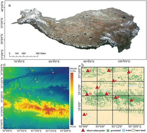
The topography of the study area, as depicted in Figure 1(b), is notably complex. The elevation within this area varies, ranging from 4,523 m to 5,119 m. The study area is square (36 km × 36 km). The boundary corresponds to the pixels in the SMAP 9-km product (Figure 1(c)), the middle yellow line is the pixel boundary of the SMAP 9-km product, and the yellow triangles mark the 10 soil moisture observation sites established in the study area (T. Zhao, Shi, et al. 2020). At the same time, the Decagon 5TM sensor is used to measure soil moisture. Table 1 shows the coordinates, elevation, soil organic matter (SOC) content (Detailed in Section 2.2.4), soil composition and soil texture (Obtained through on-site investigation) of the 10 sites.

Table 1. Information on the ground verification sites.

Site	Coordinates	Altitude (m)	Sand, silt, clay (in %)	Soil organic matter content (g/kg)	soil texture
1	93°16’11.52“E 35°18’26.13“N	4530	70.42, 24.13, 5.45	4.87	Sandy Loam
2	93°10’43.19“E 35°15’19.03“N	4561	75.33, 21.10, 3.56	5.91	Sandy Loam
3	93°4’50.78“E 35°12’56.09“N	4478	93.81, 4.84, 1.35	7.36	Sand
4	93°1’11.95“E 35°10’29.04“N	4719	59.43, 35.52, 5.04	23.53	Loam
5	93°0’13.37“E 35°3’10.59“N	4620	93.06, 5.84, 1.10	2.27	Sandy Loam
6	93°17’7.27“E 35°8’19.04“N	4634	60.10, 37.18, 2.71	138.04	Sandy Loam
7	93°11’31.28“E 35°9’19.12“N	4625	46.21, 49.68, 4.12	176.12	Silt Loam
8	93°9’1.82“E 35°19’0.90“N	4620	39.20, 48.32, 12.49	11.70	Sandy Loam
9	93°1’31.97“E 35°18’55.40“N	4700	26.88, 59.13, 13.99	11.72	Loam
10	93°8’15.15“E 35°10’36.59“N	4651	50.64, 41.95, 7.40	20.84	Loam

2.2. Data

2.2.1. Ground measured data

The Wudaoliang Soil Moisture Observation Station was inaugurated in September 2019. The observation station covers 10 soil moisture monitoring sites, the observation equipment acquires soil moisture data at various soil depths every 30 minutes, and the period of the measured soil moisture data is from September 2019 to October 2021. Considering the correspondence with the transit time of the Sentinel-1 satellite and the penetration characteristics of the C-band radar, the average of two soil moisture observations at a depth of 5 cm before and after 8:00 am was selected as the verification data.

2.2.2. Sentinel-1

Sentinel-1 carries a single C-band synthetic aperture radar (SAR) instrument, is composed of two satellites (A and B) in a near-polar orbit, and can generate continuous SAR images. Its dual-satellite system can shorten the revisit cycle from 12 days to 6 days. Sentinel data products can be downloaded from Google Earth Engine (GEE), a geospatial processing service platform provided by Google. The GEE cloud platform acquires Sentinel-1 satellite data from the official European Space Agency (ESA) website and uses the Sentinel-1 toolbox to generate calibrated and orthogonally corrected products.

2.2.3. Sentinel-2

The Sentinel-2 high-resolution multispectral imaging satellite system consists of two satellites, A and B, operating in a near-polar orbit. The double-satellite joint observation can reach a revisit period of 5 days. In this study, the Sentinel-2 L2A product provided by the GEE cloud platform was used, and 288 pieces of scene data were collected from January 2019 to December 2021. The L2A data of each scene were processed as follows: Radiometric correction and spectral correction; Top-of-atmosphere (TOA) radiation correction; Ortho-correction and resampling to the specified grid. The pixel value was converted to the surface reflectance, i.e. the bottom-of-atmosphere (BOA) correction

The cloud pixels were removed from the preprocessed data for each scene. The NDVI (Carlson and Ripley 1997) calculated from the data after removing the cloud pixels still contained anomalous values corresponding to the cloud shadows on the ground surface. To reduce the error caused by cloud shadows, based on a pixel’s NDVI time series information, images with extreme anomalies in the time series were selected and removed after they were determined to be cloud shadows. Pixels with NDVI less than 0 were mainly considered water bodies. After verification, this method can remove the pixels corresponding to the bed of the Chuma’er River and the thaw lakes. Finally, the NDVI data with a resolution of 10 m were resampled to a resolution of 100 m.

After removing clouds and cloud shadows, the original NDVI data contained a large number of null-valued pixels. NDVI represents information on vegetation growth. Since the NDVI is less variable over a short period of time, the average value for the dates adjacent to the null value was selected to replace the null value.

2.2.4. Soil organic matter data

The SOC data for the study area were from the Harmonized World Soil Database version 1.2 (HWSD). The database is jointly operated by the Food and Agriculture Organization (FAO) of the United Nations and the International Institute of Applied Systems Analysis (IIASA) in Vienna. The soil data for China in this database are from the second national land survey data released by the Institute of Soil Science, Chinese Academy of Sciences. This database provides SOC content information with a resolution of 1 km, and the data are formatted in a grid using the WGS84 projection.

3. Methodologies

3.1. Sentinel-1 SAR data processing

In this research, the 60-scene descending orbit data of the Sentinel-1A satellite from January 2019 to December 2021 were selected. The data acquisition mode used was the interferometric wide-swath (IW) mode with a spatial resolution of 5 m × 20 m and a revisit period of 12 days. GEE performed the following steps on the raw data from ESA: (1) thermal noise removal, (2) radiation correction, and (3) terrain correction based on Shuttle Radar Topography Mission (SRTM) 30-m data. Based on GEE, the images for 60 scenes were sequentially processed:

1. Refined Lee filtering for speckle noise removal.

2. Angle normalization

The radar backscatter on the ground surface is sensitive to the angle of incidence. The local incidence angle of each pixel was calculated based on the orbital parameters of Sentinel-1 and the SRTM digital elevation model (30-m resolution). For subsequent analysis with the SMAP product at the same angle, the backscatter coefficients of all pixels were normalized to 40° according to Equation (1)(1) ${\sigma }_{{\mathit{\theta }}_{\mathit{ref}}}={\sigma }_{\theta }\frac{co{s}^2{\theta }_{\mathit{ref}}}{\mathit{co}{s}^2\mathit{\theta }}$(1) .

(1) ${\sigma }_{{\mathit{\theta }}_{\mathit{ref}}}={\sigma }_{\theta }\frac{co{s}^2{\theta }_{\mathit{ref}}}{\mathit{co}{s}^2\mathit{\theta }}$(1)

In Equation (1)(1) ${\sigma }_{{\mathit{\theta }}_{\mathit{ref}}}={\sigma }_{\theta }\frac{co{s}^2{\theta }_{\mathit{ref}}}{\mathit{co}{s}^2\mathit{\theta }}$(1) , θ is the local incident angle, ${\theta }_{\mathit{ref}}$ is the normalized reference incident angle, which was set to 40° in this study, ${\sigma }_{\theta }$ is the backscatter data observed by Sentinel-1, and ${\sigma }_{{\mathit{\theta }}_{\mathit{ref}}}$is the backscatter coefficient at the reference incidence angle.

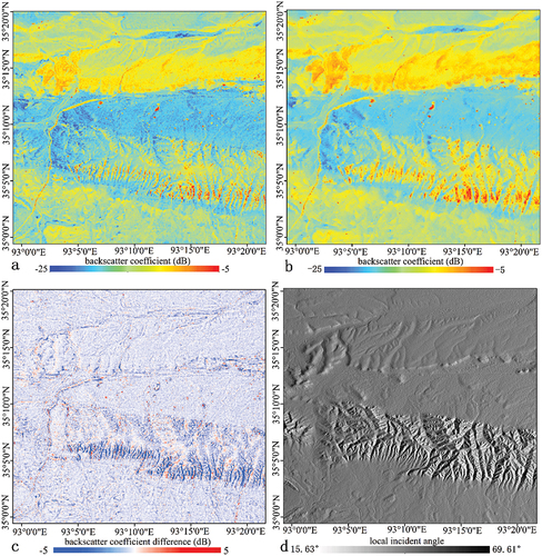
Figure 2(a) shows the spatial distribution of backscatter coefficients after angle normalization, and Figure 2(b) shows the spatial distribution of backscatter coefficients without angle normalization. The difference in local incidence angles between the two sides of the slope was large, and the backscatter differences of the corresponding pixels were mainly caused by the difference in local incidence angles rather than by differences in soil moisture. By comparing the backscatter coefficient before and after normalization, the spatial differences between the backscatter coefficients of the pixels corresponding to the hillside were improved. Figure 2(c) shows the difference in the spatial distribution of backscatter before and after angle normalization. The incident angle range of the Sentinel-1 data in the study area ranged from 32.47°-35.15°, and the local incident angle range was 15.63°-69.61° (Figure 2(c)). The overall backscatter coefficient in the study area was reduced compared to that before angle normalization, and changes were significant on both sides of the hill.

Figure 2. (a) the VV polarization data after angle normalization; (b) the VV polarization data before angle normalization; (c) the difference after and before angle normalization; (d) the local incidence angle distribution in the study area.

• (3) Averaging the backscatter coefficient to 100-m resolution

The value of each pixel at 100 m resolution was set as the average value of the corresponding 100 pixels with 10-m resolution. Compared to sampling methods, such as nearest neighbor and linear interpolation, the backscatter coefficients obtained by averaging were better correlated with soil moisture, and averaging the backscatter coefficients to 100 m resolution can reduce the speckle effect of pixels and the influence of anomalous values and can increase the stability of the data.

Finally, the processed backscatter coefficients were converted into dB units. For the vertical transmit and vertical receive (VV) polarization data, pixels with backscatter coefficients less than −24 dB or greater than −4 dB were removed.

3.2. Improved change detection method

3.2.1. Change detection method for bare soil

Backscatter from bare soil is mainly affected by soil moisture and soil surface roughness. When a change in bare soil roughness is small, the change in surface backscatter is mainly caused by the change in surface soil moisture. Therefore, soil moisture inversion can be achieved by establishing the response relationship of backscatter to soil moisture.

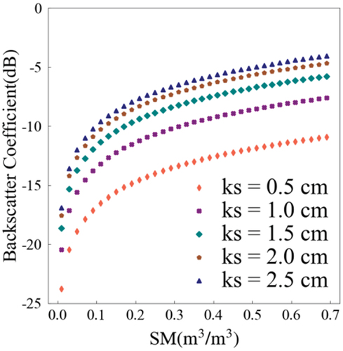
Most studies assume that the relationship between the backscatter coefficient and soil moisture is linear, and some scholars have used theoretical models to simulate the response relationship between the backscatter coefficient and soil moisture and proposed that the relationship between the two resembles an exponential relationship. In this study, the Oh semiempirical model (2004) was used for simulation. As shown in Figure 3, the incident angle was set to 40°, and the response relationships between the backscatter coefficient (VV polarization) and soil moisture under different roughness conditions were simulated. When the soil roughness and incident angle are fixed, the relationship between backscatter and soil moisture is approximately logarithmic. The sensitivity of backscatter to changes in soil moisture decreases as soil moisture increases, and this approximately logarithmic relationship between backscatter and soil moisture holds for all five simulated roughness.

Figure 3. Response of radar backscatter to soil moisture in bare soil with different soil roughness as simulated by the oh model.

Based on the simulation results, the following equation for the response of VV polarization backscatter to soil moisture in bare soil was proposed:

(2) ${\sigma }^{\mathrm{soil}}=ln\left(\mathit{SM}+\mathit{k}\right)+\mathit{D}$(2)

where ${\sigma }^{\mathrm{soil}}$is the VV polarization backscatter coefficient, SM is the surface soil water content per unit volume $({\mathrm{m}}^3/{\mathrm{m}}^3)$, and$\mathit{\hspace{0.17em}}\mathit{k}$ is the empirical coefficient related to the study area. In this research, $\mathrm{k}$ began at 0 and increased at a step of 0.05 for the soil moisture inversion simulation, and the value of k was 0.1 according to the inversion results. The D is the contribution of soil roughness to backscatter, and in this study, the change in soil roughness was ignored, so D was a constant.

In the repeated observation period, when the soil moisture reaches the maximum value ($\mathrm{S}{\mathrm{M}}_{\max }$), the backscatter reaches the maximum value ${\mathit{\sigma }}_{\max }^{\mathrm{soil}}$.

(3) ${\mathit{\sigma }}_{\max }^{\mathrm{soil}}=ln\left(\mathrm{S}{\mathrm{M}}_{\max }+\mathrm{k}\right)+\mathrm{D}$(3)

When the soil moisture reaches the minimum ($\mathrm{S}{\mathrm{M}}_{\min }$), the backscatter reaches the minimum value ${\mathit{\sigma }}_{\min }^{\mathrm{soil}}$.

(4) ${\mathit{\sigma }}_{\min }^{\mathrm{soil}}=ln\left(\mathit{S}{M}_{\mathit{min}}+\mathit{k}\right)+\mathit{D}$(4)

According to Equations (3)(3) ${\mathit{\sigma }}_{\max }^{\mathrm{soil}}=ln\left(\mathrm{S}{\mathrm{M}}_{\max }+\mathrm{k}\right)+\mathrm{D}$(3) and (4(4) ${\mathit{\sigma }}_{\min }^{\mathrm{soil}}=ln\left(\mathit{S}{M}_{\mathit{min}}+\mathit{k}\right)+\mathit{D}$(4) ), the maximum change in the backscatter coefficient within the observation period can be expressed as follows:

(5) $\mathrm{\Delta }{\mathit{\sigma }}_{\max }^{\mathrm{soil}}={\mathit{\sigma }}_{\max }^{\mathrm{soil}}-{\mathit{\sigma }}_{\min }^{\mathrm{soil}}=ln\left(\mathrm{S}{\mathrm{M}}_{\max }+\mathrm{k}\right)-ln\left(\mathrm{S}{\mathrm{M}}_{\min }+\mathrm{k}\right)$(5)

where $\mathrm{\Delta }{\mathit{\sigma }}_{\max }^{\mathrm{soil}}$ is the maximum change in backscatter within the observation period.

For the soil moisture on the t^th day in the observation period $\mathrm{S}{\mathrm{M}}_{\mathrm{t}}$ and the corresponding backscatter coefficient ${\mathit{\sigma }}_t^{\mathrm{soil}}$,

(6) $\mathrm{\Delta }{\mathit{\sigma }}_t^{\mathrm{soil}}={\mathit{\sigma }}_t^{\mathrm{soil}}-{\mathit{\sigma }}_{\min }^{\mathrm{soil}}=ln\left(\mathrm{S}{\mathrm{M}}_t+\mathrm{k}\right)-ln\left(\mathrm{S}{\mathrm{M}}_{\min }+\mathrm{k}\right)$(6)

where ${\mathit{\sigma }}_t^{\mathrm{soil}}$ is the difference between the backscatter coefficient on the t^th day and the minimum backscatter coefficient ${\mathit{\sigma }}_{\min }^{\mathrm{soil}}$ within the observation period. Therefore, according to Equations (5)(5) $\mathrm{\Delta }{\mathit{\sigma }}_{\max }^{\mathrm{soil}}={\mathit{\sigma }}_{\max }^{\mathrm{soil}}-{\mathit{\sigma }}_{\min }^{\mathrm{soil}}=ln\left(\mathrm{S}{\mathrm{M}}_{\max }+\mathrm{k}\right)-ln\left(\mathrm{S}{\mathrm{M}}_{\min }+\mathrm{k}\right)$(5) and (6(6) $\mathrm{\Delta }{\mathit{\sigma }}_t^{\mathrm{soil}}={\mathit{\sigma }}_t^{\mathrm{soil}}-{\mathit{\sigma }}_{\min }^{\mathrm{soil}}=ln\left(\mathrm{S}{\mathrm{M}}_t+\mathrm{k}\right)-ln\left(\mathrm{S}{\mathrm{M}}_{\min }+\mathrm{k}\right)$(6) ), the following expression holds:

(7) $\frac{\mathrm{\Delta }{\mathit{\sigma }}_t^{\mathrm{soil}}}{\mathrm{\Delta }{\mathit{\sigma }}_{\max }^{\mathrm{soil}}}=\frac{ln\left(\mathrm{S}{\mathrm{M}}_t+\mathrm{k}\right)-ln\left(\mathrm{S}{\mathrm{M}}_{\min }+\mathrm{k}\right)}{ln\left(\mathrm{S}{\mathrm{M}}_{\max }+\mathrm{k}\right)-ln\left(\mathrm{S}{\mathrm{M}}_{\min }+\mathrm{k}\right)}$(7)

3.2.2. Change detection method under vegetation cover

For a vegetation-covered surface, when the roughness is stable, the total surface backscatter is mainly contributed by soil moisture and vegetation. With increasing vegetation, the response sensitivity of the backscatter to the changes in soil moisture decreases. In the Wudaoliang region, the minimum backscatter occurs in winter, and the effect of vegetation on backscatter is negligible. The minimum backscatter can be expressed as ${\mathit{\sigma }}_{\min }^{\mathrm{veg}\approx 0}={\mathit{\sigma }}_{\min }^{\mathrm{soil}}$, while the maximum backscatter difference $\mathrm{\Delta }{\mathit{\sigma }}_{\max }^{\mathrm{veg}}$ is defined as follows:

(8) $\mathrm{\Delta }{\mathit{\sigma }}_{\max }^{\mathrm{veg}}={\mathit{\sigma }}_{\max }^{\mathrm{veg}}-{\mathit{\sigma }}_{\min }^{\mathrm{veg}\approx 0}={\mathit{\sigma }}_{\max }^{\mathrm{veg}}-{\mathit{\sigma }}_{\min }^{\mathrm{soil}}$(8)

where ${\mathit{\sigma }}_{\max }^{\mathrm{veg}}$ is the maximum backscatter in the observation period and veg represents the corresponding vegetation index. ${\mathit{\sigma }}_{\min }^{\mathrm{soil}}$ is the minimum backscatter, which is similar to backscatter under bare soil condition.

For a given maximum change in soil moisture $\mathrm{\Delta }\mathrm{S}{\mathrm{M}}_{\max }$, the corresponding maximum change in backscatter $\mathrm{\Delta }{\mathit{\sigma }}_{\max }^{\mathrm{veg}}$ is a function of the vegetation index:

(9) $\mathrm{\Delta }{\mathit{\sigma }}_{\max }^{\mathrm{veg}}=\mathrm{a}\cdot V_1+\mathrm{\Delta }{\mathit{\sigma }}_{\max }^{\mathrm{soil}}$(9)

$\mathrm{\Delta }{\mathit{\sigma }}_{\max }^{\mathrm{veg}}$ corresponds to the maximum difference in backscatter for the vegetation-covered surface and can be obtained from the observation data from Sentinel-1. $V_1$ represents the vegetation index corresponding to the maximum backscatter. $\mathrm{\Delta }{\mathit{\sigma }}_{\max }^{\mathrm{soil}}$ corresponds to the maximum backscatter difference under the bare soil condition. Equation (9)(9) $\mathrm{\Delta }{\mathit{\sigma }}_{\max }^{\mathrm{veg}}=\mathrm{a}\cdot V_1+\mathrm{\Delta }{\mathit{\sigma }}_{\max }^{\mathrm{soil}}$(9) indicates that when the maximum change in soil moisture$\mathrm{\Delta }\mathrm{S}{\mathrm{M}}_{\max }$is fixed, the backscatter observed by the instrument changes as the vegetation index changes.

Equation (9)(9) $\mathrm{\Delta }{\mathit{\sigma }}_{\max }^{\mathrm{veg}}=\mathrm{a}\cdot V_1+\mathrm{\Delta }{\mathit{\sigma }}_{\max }^{\mathrm{soil}}$(9) expresses the influence of vegetation on backscatter, which is valid not only for the maximum backscatter change but also for $\mathrm{\Delta }{\mathit{\sigma }}_{\mathrm{t}}^{\mathrm{veg}}$, which is under the influence of the backscatter change $\mathrm{\Delta }{\mathit{\sigma }}_{\mathrm{t}}^{\mathrm{soil}}$and the corresponding vegetation ($V_2$) on a certain day (t), and the following expression holds:

(10) $\mathrm{\Delta }{\mathit{\sigma }}_t^{\mathrm{veg}}=\mathrm{a}\cdot V_2+\mathrm{\Delta }{\mathit{\sigma }}_t^{\mathrm{soil}}$(10)

$\mathrm{\Delta }{\mathit{\sigma }}_t^{\mathrm{veg}}$ represents the change in the backscatter coefficient of a certain pixel in the study area on the t^th day relative to the backscatter coefficient of the driest condition in the observation period.$V_2$ represents the corresponding vegetation index on day t. $\mathrm{\Delta }{\mathit{\sigma }}_t^{\mathrm{soil}}$ represents the change in the backscatter coefficient of the pixel corresponding to bare soil.

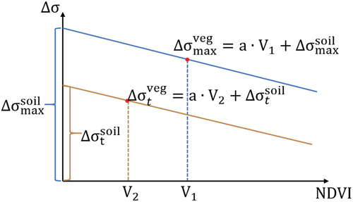
If the influence coefficient a of the vegetation on the backscatter coefficient in the study area is determined, as shown in Figure 4, the backscatter coefficient change under the influence of the vegetation and the corresponding vegetation index can be combined to obtain the change in backscatter coefficient relative to the bare soil condition. The change in the backscatter coefficient under the influence of vegetation can be calculated from the observation data from Sentinel-1. The NDVI represents the vegetation index, and NDVI is calculated from Sentinel-2 data.

Figure 4. Effect of NDVI on backscatter change.

Therefore, the backscatter change under a given NDVI can be converted to the backscatter change under the bare soil condition (i.e. NDVI = 0) through Equation (10)(10) $\mathrm{\Delta }{\mathit{\sigma }}_t^{\mathrm{veg}}=\mathrm{a}\cdot V_2+\mathrm{\Delta }{\mathit{\sigma }}_t^{\mathrm{soil}}$(10) .

According to Equations (7)(7) $\frac{\mathrm{\Delta }{\mathit{\sigma }}_t^{\mathrm{soil}}}{\mathrm{\Delta }{\mathit{\sigma }}_{\max }^{\mathrm{soil}}}=\frac{ln\left(\mathrm{S}{\mathrm{M}}_t+\mathrm{k}\right)-ln\left(\mathrm{S}{\mathrm{M}}_{\min }+\mathrm{k}\right)}{ln\left(\mathrm{S}{\mathrm{M}}_{\max }+\mathrm{k}\right)-ln\left(\mathrm{S}{\mathrm{M}}_{\min }+\mathrm{k}\right)}$(7) and (10(10) $\mathrm{\Delta }{\mathit{\sigma }}_t^{\mathrm{veg}}=\mathrm{a}\cdot V_2+\mathrm{\Delta }{\mathit{\sigma }}_t^{\mathrm{soil}}$(10) ), for pixel (i, j), the soil moisture on day t can be expressed by the following equation:

(11) $\mathrm{S}{\mathrm{M}}_t=\exp (\frac{\mathrm{\Delta }{\mathit{\sigma }}_t^{\mathrm{veg}}-\mathrm{a}\cdot {\mathrm{V}}_t}{\mathrm{\Delta }{\mathit{\sigma }}_{\max }^{\mathrm{veg}}-\mathrm{a}\cdot {\mathrm{V}}_{\max }}\left[ln\left(\mathrm{S}{\mathrm{M}}_{\max }+\mathrm{k}\right)-ln\left(\mathrm{S}{\mathrm{M}}_{\min }+\mathrm{k}\right)\right]+ln\left(\mathrm{S}{\mathrm{M}}_{\min }+\mathrm{k}\right))-\mathrm{k}$(11)

3.3. Determination of change detection method parameter

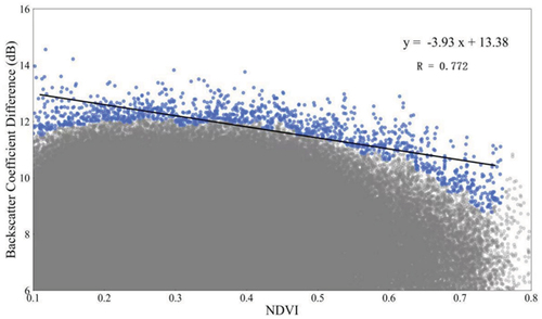
Estimation of the soil moisture inversion requires determination of the influence coefficient a of vegetation on backscatter in Equation (9)(9) $\mathrm{\Delta }{\mathit{\sigma }}_{\max }^{\mathrm{veg}}=\mathrm{a}\cdot V_1+\mathrm{\Delta }{\mathit{\sigma }}_{\max }^{\mathrm{soil}}$(9) . Figure 5 shows the trend of backscatter under different NDVIs in the study area. Pixels with NDVI less than 0.1 or greater than 0.75 were removed. To determine the coefficient a, NDVI was divided into continuous cells with an interval of 0.015, the largest fraction of the backscatter in each cell was taken as the maximum backscatter change for that cell, and all the maximum values within the NDVI range of 0.1–0.75 were obtained (Figure 5). After linearly fitting the maximum values, the relationship between the maximum backscatter and NDVI was obtained. In the study area, the influence coefficient of vegetation on backscatter was a = −3.93.

Figure 5. Trend of backscatter change under different NDVIs in the study area. The ordinate of each point represents the difference between the backscatter of the pixel on a certain day and the minimum backscatter of the pixel during the observation period. The abscissa is the NDVI at that time. As NDVI increases, the backscatter declines.

The change detection method retrieves the soil moisture changes from the change in backscatter. To retrieve the absolute value of soil moisture, it is necessary to determine the minimum soil moisture $\mathrm{S}{\mathrm{M}}_{\min }$ and maximum soil moisture $\mathrm{S}{\mathrm{M}}_{\max }$ in the observation period.

When soil moisture is low, it corresponds to low backscatter. In addition, soil moisture affects the growth and development of vegetation, which in turn affects the organic matter content in the soil. The minimum VV polarization backscatter ($\mathrm{V}{\mathrm{V}}_{\min }$), minimum NDVI ($\mathrm{NDV}{\mathrm{I}}_{\min }$), and the SOC content at 10 sites within the observation period were used to build an empirical relationship to fit the minimum soil moisture values at 10 sites. The empirical relationship of the minimum soil moisture is shown in Equation (12)(12) $\mathrm{S}{\mathrm{M}}_{\min }=3.94\mathit{\hspace{0.17em}}\bullet {10}^{-3}\mathrm{V}{\mathrm{V}}_{\min }+1.77\bullet {10}^2(\mathrm{NDV}{\mathrm{I}}_{\min }{)}^3+5.17\bullet {10}^{-4}\mathrm{SOC}+8.32\bullet {10}^{-2}$(12) :

(12) $\mathrm{S}{\mathrm{M}}_{\min }=3.94\mathit{\hspace{0.17em}}\bullet {10}^{-3}\mathrm{V}{\mathrm{V}}_{\min }+1.77\bullet {10}^2(\mathrm{NDV}{\mathrm{I}}_{\min }{)}^3+5.17\bullet {10}^{-4}\mathrm{SOC}+8.32\bullet {10}^{-2}$(12)

When fitting the maximum soil moisture change, the maximum VV-VH difference of the pixel in the observation period was added, and the obtained empirical relationship is expressed by Equation (13)(13) $\mathrm{\Delta }\mathrm{S}{\mathrm{M}}_{\max }=-0.0178\bullet \mathrm{\Delta }\mathrm{V}{\mathrm{V}}_{\max }+0.28\bullet {\left(\mathrm{\Delta }\mathrm{NDV}{\mathrm{I}}_{\max }\right)}^3+8.05\bullet {10}^{-4}\mathrm{SOC}+0.027\mathrm{\Delta }{\left(\mathrm{VV}-\mathrm{VH}\right)}_{\max }+0.129$(13) :

(13) $\mathrm{\Delta }\mathrm{S}{\mathrm{M}}_{\max }=-0.0178\bullet \mathrm{\Delta }\mathrm{V}{\mathrm{V}}_{\max }+0.28\bullet {\left(\mathrm{\Delta }\mathrm{NDV}{\mathrm{I}}_{\max }\right)}^3+8.05\bullet {10}^{-4}\mathrm{SOC}+0.027\mathrm{\Delta }{\left(\mathrm{VV}-\mathrm{VH}\right)}_{\max }+0.129$(13)

The maximum soil moisture at each site $\mathrm{S}{\mathrm{M}}_{\max }$ can be obtained from Equation (14)(14) $\mathrm{S}{\mathrm{M}}_{\max }=\mathrm{S}{\mathrm{M}}_{\min }+\mathrm{\Delta }\mathrm{S}{\mathrm{M}}_{\max }$(14) .

(14) $\mathrm{S}{\mathrm{M}}_{\max }=\mathrm{S}{\mathrm{M}}_{\min }+\mathrm{\Delta }\mathrm{S}{\mathrm{M}}_{\max }$(14)

Then, these site-specific models and parameters were used to generate auxiliary data for subsequent change detection algorithms.

4. Results

4.1. Validation with ground measurements

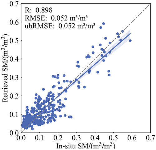
The minimum and maximum values of soil moisture, as determined by the change detection method, were utilized to retrieve the soil moisture. The results of the soil moisture inversion, at a resolution of 100 meters corresponding to the 10 observation sites, were then compared with the data from ground observations. As shown in Figure 6, the maximum soil moisture at the 10 sites reached 0.602$m^3/m^3$, and the change detection method showed good performance since the coefficient of correlation between the inversion and measured values reached 0.898, and the RMSE attained 0.052 $m^3/m^3$.

Figure 6. Comparison of ground observations and inversion results in the Wudaoliang region.

As shown in Figure 7, the soil moisture at the 10 observation sites fluctuated significantly throughout the year. In winter, the soil moisture changed steadily, and the maximum value did not exceed 0.1$m^3/m^3$; in May, as the temperature increased and the frozen soil melted, the soil moisture at all 10 observation sites began to increase.

Figure 7. Comparison between the soil moisture retrieved by the change detection method and that estimated by ground measurement data. Each blue dot in the figure represents the soil moisture inversion data (100-m resolution) corresponding to the ground observation site, and the gray line represents the ground observation value.

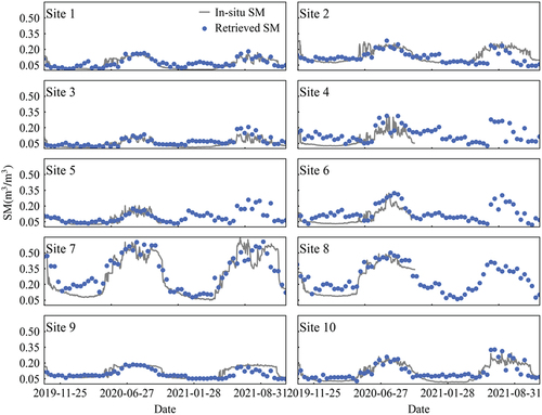
The soil moisture retrieved by the change detection method can express the soil moisture trend during two year at the 10 sites. Table 2 shows the statistical parameters of the relationship between the inversion values and the ground observation values of the 10 sites. For the 10 sites, the retrieved soil moisture values correlated well with the ground observation values. Site 2 had the smallest correlation coefficient (R = 0.619) and the largest RMSE (0.058 $m^3/m^3$) among the 10 sites, and for the Site 2, the minimum soil moisture varied considerably from the ground observations, which is the reason for the large difference between the inversion results and the ground observation results at Site 2. This result indicates that the accurate measurement of the minimum soil moisture in the change detection algorithm is critical to the soil moisture inversion results. The correlation coefficients of the other nine ground observation sites all reached or approached 0.8, which indicates that this method retains good applicability in the areas with high soil moisture.

Table 2. Comparison of statistical parameters of inversion and measured results at 10 sites in the Wudaoliang region.

Site	1	2	3	4	5	6	7	8	9	10
R	0.767	0.619	0.798	0.799	0.814	0.784	0.867	0.943	0.777	0.836
RMSE(m^3/m^3)	0.034	0.058	0.033	0.073	0.030	0.073	0.102	0.072	0.036	0.046
ubRMSE(m^3/m^3)	0.032	0.055	0.026	0.045	0.029	0.051	0.096	0.049	0.033	0.045

The soil moisture retrieved by the change detection method in winter was overestimated relative to the ground observation data, and the retrieved soil moisture showed relatively obvious fluctuations. The Wudaoliang region belongs to the permafrost area, the soil is frozen in winter, and water is mainly stored in the soil in the form of ice, while the retrieved soil water in this study was free water. The soil moisture was lower than 0.1 $m^3/m^3$ at all 10 ground observation sites, and in winter, the effect of surface roughness on the backscatter coefficient exceeded that of soil moisture. In the Wudaoliang region, the annual average wind speed is 4.1 m/s, and the maximum wind speed can reach 40 m/s; in addition, the soil is dry in winter, the particles in the soil surface layer could be spatially redistributed by strong winds, resulting in a change in soil roughness and thereby causing a large change in backscatter. This overestimation may be caused by multiple factors, not only the influence of wind on roughness, but also vegetation or human factors (Zhu et al. 2019). All these mechanisms are reasons for the large fluctuation in the soil moisture inversion results in winter.

In summer, soil moisture was the main factor affecting backscatter. The maximum soil moisture values varied substantially among sites, and the inversion values at different sites could effectively express the trend in soil moisture.

Significant underestimation of soil moisture occurred at the 10 stations during the periods from April-May and September-October, and underestimation of soil moisture occurred at all sites, indicating that the change in land surface cover was not the main factor in the underestimation. During these two periods, the temperature changes more drastically, the surface soil changes from freezing to thawing or from thawing to freezing, and the freezing and thawing could cause sedimentation or frost heaving of the soil in the study area, which changes the soil roughness to a certain extent.

4.2. Comparison with SMAP 9-km product

To further evaluate the retrieved soil moisture, the SMAP 9-km product was used for comparison, as shown in Figure 8 (left panel). The blue points represent the retrieved average soil moisture across the entire study area (36 km × 36 km) at 100 m resolution, the red points represent the averages of the 16 SMAP 9-km product grids corresponding to the study area, and the gray curve represents the average soil moisture obtained from the 10 ground observation sites. The black vertical line represents the average rainfall in the study area. The rainfall data are from the Climate Hazards Group InfraRed Precipitation with Station data (CHIRPS) dataset provided by the GEE platform, and the CHIRPS dataset combines 0.05° resolution satellite imagery with ground observation data to create gridded rainfall time series, which can be used for trend analysis and seasonal drought monitoring.

Figure 8. The left panel shows the comparison of the time series of the inversion values obtained by the change detection method (blue dots), the ground observation values (gray curve), and the SMAP product results (red dots). The right panel shows the comparison between the inversion value obtained by the change detection method and the SMAP product results.

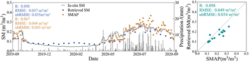
Across the entire study area, soil moisture changes were clearly driven by rainfall. In winter, the soil moisture was stable at 0.05 $m^3/m^3$. From April-May, as the rainfall increased, the soil gradually became wet. The rainfall in this area is concentrated in the period from June-August, and the soil moisture reached a maximum value of 0.287 $m^3/m^3$ then. At the 36-km scale, the retrieved soil moisture was strongly correlated with the ground observations, with a correlation coefficient of R = 0.898 and an RMSE = 0.037$m^3/m^3$. The coefficient of correlation between the SMAP 9-km product and the ground observation values in this area was R = 0.867, and the RMSE = 0.044 $m^3/m^3$. The soil moisture retrieved using the change detection method was superior to that from the SMAP 9-km product. In general, the SMAP 9-km product overestimated the soil moisture in summer, and in particular, on 9 August 2020, the value of 0.367 $m^3/m^3$ was much higher than the ground observation result (0.248$\mathit{\hspace{0.17em}}{\mathrm{m}}^3/{\mathrm{m}}^3$). The SMAP 9-km product underestimated soil moisture in spring and fall. Figure 8 (right panel) shows the comparison between the retrieved soil moisture and that from the SMAP product during the same period. At the 36-km scale, the correlation coefficient of the two was R = 0.898, and the RMSE was 0.049 ${\mathrm{m}}^3/{\mathrm{m}}^3$. Despite the disparities between the two retrieved soil moisture (underestimated for Sentinel-1, overestimated for SMAP), the method proposed in this study is deemed reliable owing to their relatively robust correlation.

4.3. Comparison with SMAP 9-km product spatiotemporal distribution

The first column of Figure 9 shows the spatial distribution of soil moisture during the four periods retrieved by the change detection method. In terms of spatial distribution, soil moisture is highest in the central portion, with the wetter areas concentrated in the valleys of the central hills and the highland swampy meadows on the northern slopes of the hills. The soil moisture is stably maintained at 0.25 $m^3/m^3$and above, and dense vegetation weakens the evapotranspiration, the soil retains more moisture.

Figure 9. The first column shows the spatial distribution of soil moisture at different times in the study area retrieved by the change detection method, and the second column shows the SMAP 9-km product results derived from the same data used in the change detection method.

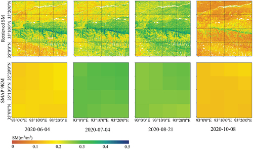
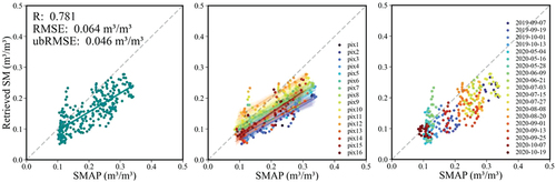
Regarding temporal distribution, the retrieved soil moisture initially increases and subsequently decreases across the entire study area. This pattern aligns with the results from the SMAP 9-km product. However, the spatial change in the SMAP 9-km product results prevents it from accurately reflecting the spatial variation in soil moisture. The retrieved soil moisture and SMAP 9-km product results were compared at the 9-km scale (Figure 10). The left panel shows the comparison between the values for each grid from SMAP 9-km and the inversion values of the corresponding area; the correlation coefficient is R = 0.781, and the RMSE is 0.064 $m^3/m^3$. The middle panel shows the time series data for 16 grids from the SMAP 9-km product, and different colors represent different grids. For each 9-km grid in the study area, the retrieved soil moisture and SMAP 9-km product results were strongly correlated in the time series, i.e. both can express the time series variation of soil moisture in the study area. In the right panel, different colors represent different dates, and points of the same color represent the inversion data and SMAP 9-km data for the same grid in the study area on a certain day. On one day, the spatial distribution of the SMAP 9-km product showed a small change, while the 100-m resolution soil moisture obtained by the change detection method exhibited a broader range of changes, which indicates that the change detection method can better express the heterogeneity of the spatial distribution of soil moisture in this area.

Figure 10. The left panel shows the comparison of the inversion results of the change detection method and SMAP 9-km product results, the middle panel represents the comparison of soil moisture values with SMAP 9-km product results within each 9-km grid (pix represents grid), and the right panel shows the comparison of the distribution of the inversion values for the change detection method and the distribution of the SMAP 9-km product results in different days.

5. Discussion

In this research, the change detection method was improved as follows: First, using the Oh empirical model, the response of backscatter to soil moisture in bare soil was expressed in logarithmic form. Compared to previous studies that focused more on assuming a linear function relationship (Hahn et al. 2021; Hornacek et al. 2012), this study is more convincing by simulating a logarithmic function relationship based on a physical model. Secondly, the maximum backscatter difference and NDVI of each pixel in the study area were used to establish the empirical relationship between the two, and then the backscatter differences under the vegetation cover condition were corrected to the backscatter differences under the bare soil condition. However, the empirical function relationship established in this study is only applicable to the vegetation change in the range of 0.1–0.75. If NDVI is less than 0.1, the bare soil change detection algorithm is used. If NDVI is higher than 0.75, due to the dense vegetation, the microwave signal is difficult to penetrate the dense vegetation, and the calculated soil moisture also has a certain error.

In order to obtain the absolute values of soil moisture, we established two sets of empirical equations by inputting a series of auxiliary data to obtain the minimum and maximum changes in soil moisture. Firstly, because the research area is located in the Qinghai-Tibet Plateau, this study also considered that the radar backscatter value will fluctuate significantly during the freeze-thaw period due to the influence of soil roughness during this period. Therefore, the average soil moisture measured by the instrument during this period is used as the reference for unfrozen water, and the corresponding average radar backscatter value during this period is used as the reference for backscatter. Why not take the soil moisture at the critical point of freeze-thaw conversion, because this critical period is difficult to determine, and the freeze-thaw critical periods of each pixel are not synchronized. Secondly, there is also some uncertainty in the SOC data itself, and we further incorporate auxiliary data such as NDVI into it to reduce uncertainty. At the same time, considering the special area of the Qinghai-Tibet Plateau, the type of vegetation cover is single, mostly grassland or bare soil, which can also better improve the reliability of the empirical equations we built.

The change detection method relies on the assumption that the soil roughness remains constant throughout the observation period. However, in reality, the soil roughness could be subject to change. Since the study area is located in the permafrost region of the Qinghai-Tibet Plateau, the seasonal freeze-thaw transition of the surface soil in this area could cause surface uplift or subsidence, resulting in alterations to the surface roughness. In this study, the change in surface roughness was ignored. The change detection method overestimates soil moisture in winter, and we believe that the soil roughness change due to the redistribution of soil surface particles caused by the freeze-thaw processes and strong winds in winter is the reason.

Therefore, in future studies, the change in backscatter coefficient due to soil roughness should be considered, which would improve the accuracy of inversion change detection algorithms. To eliminate the influence of vegetation, the optical data were used to calculate the NDVI when establishing the empirical function; however, the complete NDVI distribution in this area cannot be obtained due to the influence of clouds. In future studies, the use of vegetation indices based on active radar data could be considered to address the null-valued pixels caused by clouds.

6. Conclusions

The improved change detection method was validated using the data obtained at the surface soil moisture observation stations in the Wudaoliang permafrost region of the Qinghai-Tibet Plateau, and the improved change detection method exhibited high correlations at all 10 surface observation sites and could sensitively capture changes in soil moisture caused by rainfall over a short period of time. Compared with the SMAP 9-km product, the change detection algorithm displayed a better correlation (R = 0.898 and R = 0.867) and a lower RMSE (RMSE = 0.037 $m^3/m^3$ and RMSE = 0.044$m^3/m^3$, respectively) in the study area. The retrieved soil moisture and SMAP 9-km product results were strongly correlated in the time series. The 100-m resolution soil moisture obtained by the change detection method exhibited a broader range of changes, which indicates that the change detection method can better express the heterogeneity of the spatial distribution of soil moisture in this area.

Acknowledgments

The authors would like to thank the European Space Agency for providing free Sentinel-1 data

Disclosure statement

No potential conflict of interest was reported by the author(s).

Data availability statement

The results of this study can be downloaded https://cstr.cn/18406.11.Terre.tpdc.301067.

Additional information

Funding

This study was jointly supported by the National Key Research and Development Program of China [No. 2022YFB3903302] and the National Natural Science Foundation of China [No. 42201393].

References

- Bai, X., B. He, and X. Li. 2015. “Optimum Surface Roughness to Parameterize Advanced Integral Equation Model for Soil Moisture Retrieval in Prairie Area Using Radarsat-2 Data.” IEEE Transactions on Geoscience and Remote Sensing 54 (4): 2437–17. https://doi.org/10.1109/TGRS.2015.2501372.
- Barrett, B. W., E. Dwyer, and P. Whelan. 2009. “Soil Moisture Retrieval from Active Spaceborne Microwave Observations: an Evaluation of Current Techniques.” Remote Sensing 1:210–242. https://doi.org/10.3390/rs1030210.
- Bhogapurapu, N., S. Dey, D. Mandal, A. Bhattacharya, L. Karthikeyan, H. McNairn, and Y. S. Rao. 2022. “Soil Moisture Retrieval Over Croplands Using Dual-Pol L-Band GRD SAR Data.” Remote Sensing of Environment 271:112900. https://doi.org/10.1016/j.rse.2022.112900.
- Bindlish, R., and A. P. Barros. 2000. “Multifrequency Soil Moisture Inversion from SAR Measurements with the Use of IEM.” Remote Sensing of Environment 71 (1): 67–88. https://doi.org/10.1016/S0034-4257(99)00065-6.
- Carlson, T. N., and D. A. Ripley. 1997. “On the Relation Between NDVI, Fractional Vegetation Cover, and Leaf Area Index.” Remote Sensing of Environment 62 (3): 241–252. https://doi.org/10.1016/S0034-4257(97)00104-1.
- Champagne, C., A. Berg, J. Belanger, H. McNairn, and R. De Jeu. 2010. “Evaluation of Soil Moisture Derived from Passive Microwave Remote Sensing Over Agricultural Sites in Canada Using Ground-Based Soil Moisture Monitoring Networks.” International Journal of Remote Sensing 31 (14): 3669–3690. https://doi.org/10.1080/01431161.2010.483485.
- Chen, K., T. D. Wu, L. Tsang, Q. Li, J. Shi, and A. K. Fung. 2003. “Emission of Rough Surfaces Calculated by the Integral Equation Method with Comparison to Three-Dimensional Moment Method Simulations.” IEEE Transactions on Geoscience and Remote Sensing: A Publication of the IEEE Geoscience and Remote Sensing Society 41:90–101. https://doi.org/10.1109/TGRS.2002.807587.
- Fan, D., T. Zhao, X. Jiang, H. Xue, S. Moukomla, K. Kuntiyawichai, and J. Shi. 2021. “Soil Moisture Retrieval from Sentinel-1 Time-Series Data Over Croplands of Northeastern Thailand.” IEEE Geoscience and Remote Sensing Letters 19:1–5. https://doi.org/10.1109/LGRS.2021.3065868.
- Fung, A. K., and K. S. Chen. 2004. “An Update on the IEM Surface Backscattering Model.” IEEE Geoscience and Remote Sensing Letters 1 (2): 75–77. https://doi.org/10.1109/LGRS.2004.826564.
- Fung, A., Z. Li, and K. Chen. 1992. “Backscattering from a Randomly Rough Dielectric Surface.” IEEE Transactions on Geoscience and Remote Sensing: A Publication of the IEEE Geoscience and Remote Sensing Society 30:356–369. https://doi.org/10.1109/36.134085.
- Gao, Q., M. Zribi, M. J. Escorihuela, and N. Baghdadi. 2017. “Synergetic Use of Sentinel-1 and Sentinel-2 Data for Soil Moisture Mapping at 100 M Resolution.” Sensors 17:1966. https://doi.org/10.3390/s17091966.
- Hahn, S., W. Wagner, S. C. Steele-Dunne, M. Vreugdenhil, and T. Melzer. 2021. “Improving ASCAT Soil Moisture Retrievals with an Enhanced Spatially Variable Vegetation Parameterization.” IEEE Transactions on Geoscience and Remote Sensing 59 (10): 8241–8256. https://doi.org/10.1109/TGRS.2020.3041340.
- Hornacek, M., W. Wagner, D. Sabel, H. L. Truong, P. Snoeij, T. Hahmann, E. Diedrich, and M. Doubková. 2012. “Potential for High Resolution Systematic Global Surface Soil Moisture Retrieval via Change Detection Using Sentinel-1.” IEEE Journal of Selected Topics in Applied Earth Observations and Remote Sensing 5 (4): 1303–1311. https://doi.org/10.1109/JSTARS.2012.2190136.
- Hosseini, M., and H. McNairn. 2017. “Using Multi-Polarization C-And L-Band Synthetic Aperture Radar to Estimate Biomass and Soil Moisture of Wheat Fields.” International Journal of Applied Earth Observation and Geoinformation 58:50–64. https://doi.org/10.1016/j.jag.2017.01.006.
- Ines, A. V. M., N. N. Das, J. W. Hansen, and E. G. Njoku. 2013. “Assimilation of Remotely Sensed Soil Moisture and Vegetation with a Crop Simulation Model for Maize Yield Prediction.” Remote Sensing of Environment 138:149–164. https://doi.org/10.1016/j.rse.2013.07.018.
- Kim, S., K. Paik, F. Johnson, and A. Sharma. 2018. “Building a Flood-Warning Framework for Ungauged Locations Using Low Resolution, Open-Access Remotely Sensed Surface Soil Moisture, Precipitation, Soil, and Topographic Information.” IEEE Journal of Selected Topics in Applied Earth Observations & Remote Sensing 11 (2): 375–387. https://doi.org/10.1109/JSTARS.2018.2790409.
- Kim, Y., and J. J. Van Zyl. 2009. “A Time-Series Approach to Estimate Soil Moisture Using Polarimetric Radar Data.” IEEE Transactions on Geoscience and Remote Sensing 47 (8): 2519–2527. https://doi.org/10.1109/TGRS.2009.2014944.
- Laiolo, P., S. Gabellani, L. Campo, F. Silvestro, F. Delogu, R. Rudari, L. Pulvirenti, et al. 2016. “Impact of Different Satellite Soil Moisture Products on the Predictions of a Continuous Distributed Hydrological Model.” International Journal of Applied Earth Observation and Geoinformation: ITC Journal 48:131–145. https://doi.org/10.1016/j.jag.2015.06.002.2015.06.002.
- Legates, D. R., R. Mahmood, D. F. Levia, T. L. DeLiberty, S. M. Quiring, C. Houser, and F. E. Nelson. 2011. “Soil Moisture: A Central and Unifying Theme in Physical Geography.” Progress in Physical Geography: Earth and Environment 35 (1): 65–86. https://doi.org/10.1177/0309133310386514.
- Li, X., A. Al-Yaari, M. Schwank, L. Fan, F. Frappart, J. Swenson, and J. P. Wigneron. 2020. “Compared Performances of SMOS-IC Soil Moisture and Vegetation Optical Depth Retrievals Based on Tau-Omega and Two-Stream Microwave Emission Models.” Remote Sensing of Environment 236:111502. https://doi.org/10.1016/j.rse.2019.111502.
- Lievens, H., and N. Verhoest. 2011. “On the Retrieval of Soil Moisture in Wheat Fields from L-Band SAR Based on Water Cloud Modeling, the IEM, and Effective Roughness Parameters.” IEEE Geoscience & Remote Sensing Letters 8 (4): 740–744. https://doi.org/10.1109/LGRS.2011.2106109.
- Liu, Y., J. Qian, and H. Yue. 2020. “Combined Sentinel-1A with Sentinel-2A to Estimate Soil Moisture in Farmland.” IEEE Journal of Selected Topics in Applied Earth Observations and Remote Sensing 14:1292–1310. https://doi.org/10.1109/JSTARS.2020.3043628.
- Li, X., J. P. Wigneron, L. Fan, F. Frappart, S. H. Yueh, A. Colliander, A. Ebtehaj, et al. 2022. “A New SMAP Soil Moisture and Vegetation Optical Depth Product (SMAP-IB): Algorithm, Assessment and Inter-Comparison.” Remote Sensing of Environment 271:112921. https://doi.org/10.1016/j.rse.2022.112921.
- Ma, C., X. Li, and M. F. McCabe. 2020. “Retrieval of High-Resolution Soil Moisture Through Combination of Sentinel-1 and Sentinel-2 Data.” Remote Sensing 12:2303. https://doi.org/10.3390/rs12142303.
- Merzouki, A., H. McNairn, and A. Pacheco. 2011. “Mapping Soil Moisture Using RADARSAT-2 Data and Local Autocorrelation Statistics.” IEEE Journal of Selected Topics in Applied Earth Observations & Remote Sensing 4 (1): 128–137. https://doi.org/10.1109/JSTARS.2011.2116769.
- Paloscia, S., S. Pettinato, E. Santi, C. Notarnicola, L. Pasolli, and A. Reppucci. 2013. “Soil Moisture Mapping Using Sentinel-1 Images: Algorithm and Preliminary Validation.” Remote Sensing of Environment 134:234–248. https://doi.org/10.1016/j.rse.2013.02.027.
- Robinson, D. A., C. S. Campbell, J. W. Hopmans, B. K. Hornbuckle, S. B. Jones, R. Knight, F. Ogden, J. Selker, and O. Wendroth. 2008. “Soil Moisture Measurement for Ecological and Hydrological Watershed-Scale Observatories: A Review.” Vadose Zone Journal 7:358–389. https://doi.org/10.2136/vzj2007.0143.
- Rowlandson, T., S. Impera, J. Belanger, A. A. Berg, B. Toth, and R. Magagi. 2015. “Use of In Situ Soil Moisture Network for Estimating Regional-Scale Soil Moisture During High Soil Moisture Conditions.” Canadian Water Resources Journal/Revue Canadienne des Ressources Hydriques 40 (4): 343–351. https://doi.org/10.1080/07011784.2015.1061948.
- Seneviratne, S. I., T. Corti, E. L. Davin, M. Hirschi, E. B. Jaeger, I. Lehner, B. Orlowsky, and A. J. Teuling. 2010. “Investigating Soil Moisture–Climate Interactions in a Changing Climate: A Review.” Earth Science Review 99 (3–4): 125–161. https://doi.org/10.1016/j.earscirev.2010.02.004.
- Seneviratne, S. I., M. Wilhelm, T. Stanelle, B. Van den Hurk, S. Hagemann, A. Berg, F. Cheruy, et al. 2013. “Impact of Soil Moisture-Climate Feedbacks on CMIP5 Projections: First Results from the GLACE-CMIP5 Experiment.” Geophysical Research Letters 40:5212–5217. https://doi.org/10.1002/grl.50956.
- Shi, J., Y. Du, J. Du, L. Jiang, L. Chai, K. Mao, P. Xu, et al. 2012. “Progresses on Microwave Remote Sensing of Land Surface Parameters.” Scientia Sinica (Terrae) 42:814–842. https://doi.org/10.1007/s11430-012-4444-x.
- Singh, A., K. Gaurav, G. K. Meena, and S. Kumar. 2020. “Estimation of Soil Moisture Applying Modified Dubois Model to Sentinel-1, a Regional Study from Central India.” Remote Sensing 12 (14): 2266. https://doi.org/10.3390/rs12142266.
- Ulaby, F. T., R. K. Moore, and A. K. Fung. 1981. Microwave Remote Sensing: Active and Passive. Reading, MA: Addison- Wesley Publishers.
- Vereecken, H., J. A. Huisman, Y. Pachepsky, C. Montzka, J. Van der Kruk, H. Bogena, L. Weihermüller, M. Herbst, G. Martinez, and J. Vanderborght. 2014. “On the Spatio-Temporal Dynamics of Soil Moisture at the Field Scale.” Canadian Journal of Fisheries and Aquatic Sciences 516:76–96. https://doi.org/10.1016/j.jhydrol.2013.11.061.
- Wagner, W., G. Lemoine, and H. Rott. 1999. “A Method for Estimating Soil Moisture from ERS Scatterometer and Soil Data.” Remote Sensing of Environment 70:191–207. https://doi.org/10.1016/S0034-4257(99)00036-X.
- Wang, Z., T. Zhao, J. Shi, H. Wang, D. Ji, P. Yao, J. Zheng, X. Zhao, and X. Xu. 2023. “1-Km Soil Moisture Retrieval Using Multi-Temporal Dual-Channel SAR Data from Sentinel-1 A/B Satellites in a Semi-Arid Watershed.” Remote Sensing of Environment 284:113334. https://doi.org/10.1016/j.rse.2022.113334.
- Weimann, A., M. Von Schonermark, A. Schumann, P. Jorn, and R. Gunther. 1998. “Soil Moisture Estimation with ERS-1 SAR Data in the East-German Loess Soil Area.” International Journal of Remote Sensing 19:237–243. https://doi.org/10.1080/014311698216224.
- Xing, M., B. He, X. Ni, J. Wang, G. An, J. Shang, and X. Huang. 2019. “Retrieving Surface Soil Moisture Over Wheat and Soybean Fields During Growing Season Using Modified Water Cloud Model from Radarsat-2 SAR Data.” Remote Sensing 11 (16): 1956. https://doi.org/10.3390/rs11161956.
- Yadav, V. P., R. Prasad, R. Bala, and A. K. Vishwakarma. 2020. “An Improved Inversion Algorithm for Spatio-Temporal Retrieval of Soil Moisture Through Modified Water Cloud Model Using C-Band Sentinel-1A SAR Data.” Computers and Electronics in Agriculture 173:105447. https://doi.org/10.1016/j.compag.2020.105447.
- Zhang, K., Q. Wang, L. Chao, J. Ye, Z. Li, Z. Yu, T. Yang, and Q. Ju. 2019. “Ground Observation-Based Analysis of Soil Moisture Spatiotemporal Variability Across a Humid to Semi-Humid Transitional Zone in China.” Canadian Journal of Fisheries and Aquatic Sciences 574:903–914. https://doi.org/10.1016/j.jhydrol.2019.04.087.
- Zhao, T., L. Hu, J. Shi, H. Lü, S. Li, D. Fan, P. Wang, D. Geng, C. S. Kang, and Z. Zhang. 2020. “Soil Moisture Retrievals Using L-Band Radiometry from Variable Angular Ground-Based and Airborne Observations.” Remote Sensing of Environment 248:111958. https://doi.org/10.1016/j.rse.2020.111958.
- Zhao, T., J. Shi, L. Lv, H. Xu, D. Chen, Q. Cui, T. Jackson, et al. 2020. “Soil Moisture Experiment in the Luan River Supporting New Satellite Mission Opportunities.” Remote Sensing of Environment 240:111680. https://doi.org/10.1016/j.rse.2020.111680.
- Zhao, H., Y. Zeng, J. G. Hofste, T. Duan, J. Wen, and Z. Su. 2022. “Modelling of Multi-Frequency Microwave Backscatter and Emission of Land Surface by a Community Land Active Passive Microwave Radiative Transfer Modelling Platform (CLAP).” Hydrology & Earth System Sciences Discussions 1–48. https://doi.org/10.5194/hess-2022-333.
- Zhu, L., R. Si, X. Shen, and J. P. Walker. 2022. “An Advanced Change Detection Method for Time-Series Soil Moisture Retrieval from Sentinel-1.” Remote Sensing of Environment 279:113137. https://doi.org/10.1016/j.rse.2022.113137.
- Zhu, L., J. P. Walker, N. Ye, and C. Rüdiger. 2019. “Roughness and Vegetation Change Detection: A Pre-Processing for Soil Moisture Retrieval from Multi-Temporal SAR Imagery.” Remote Sensing of Environment 225:93–106. https://doi.org/10.1016/j.rse.2019.02.027.
- Zhu, L., S. Yuan, Y. Liu, C. Chen, and J. P. Walker. 2023. “Time Series Soil Moisture Retrieval from SAR Data: Multi-Temporal Constraints and a Global Validation.” Remote Sensing of Environment 287:113466. https://doi.org/10.1016/j.rse.2023.113466.
- Zribi, M., C. Andre, and B. Decharme. 2008. “A Method for Soil Moisture Estimation in Western Africa Based on the ERS Scatterometer.” IEEE Transactions on Geoscience & Remote Sensing 46 (2): 438–448. https://doi.org/10.1109/TGRS.2007.904582.
- Zribi, M., and M. Dechambre. 2003. “A New Empirical Model to Retrieve Soil Moisture and Roughness from C-Band Radar Data.” Remote Sensing of Environment 84 (1): 42–52. https://doi.org/10.1016/S0034-4257(02)00069-X.