Cross-comparison of Landsat-8 and Landsat-9 data: a three-level approach based on underfly images

ABSTRACT

The recently launched Landsat-9 has an important mission of working together with Landsat-8 to reduce the revisit period of Landsat Earth observations to eight days. This requires the data of Landsat-9 to be highly consistent with that of Landsat-8 to avoid bias caused by data inconsistency when the two satellites are simultaneously used. Therefore, this study evaluated the consistency of the surface reflectance (SR) and land surface temperature (LST) data between Landsat-8 and Landsat-9 based on five test sites from different parts of the world using synchronized underfly image pairs of both satellites. Previous cross-comparisons have demonstrated high consistency between the spectral bands of Landsat-8 and Landsat-9, with differences of around 1%. However, it is unclear whether this low deviation will be amplified in subsequent multiband calculations. It is also necessary to determine whether the difference is consistent across different land cover types. Therefore, this study used a three-level cross-comparison approach to specifically examine these concerns. Besides the commonly used band-by-band comparison, which served as the first-level comparison in this study, this approach included a second-level comparison based on the calculations of several indicators and a third-level comparison based on a composite index calculated from the indicators obtained in the second-level comparison. This three-level approach will examine whether the difference found in the first-level per-band comparison would change after the subsequent calculations in the second- and third-level comparisons. The Remote Sensing based Ecological Index (RSEI) was used for this approach because it is a composite index integrating four indicators. The results of this three-level comparison show that the first-level per-band comparison exhibited high consistency between the two satellites’ SR data, with an average absolute percent change (PC) of 1.88% and an average R² of 0.957 across six bands in the five test sites. This deviation increased to 2.21% in the third-level composite index-based comparison, with R² decreasing to 0.956. This indicates that after complex calculations, the deviation between the bands of the two satellites was amplified to some extent. However, when analyzing specific land cover types, notable differences emerged between the two satellites for the water category, with an average absolute PC ranging from 18% to 35% and an R² of lower than 0.6. Additionally, there were also nearly 5% differences for the built-up land category, with an average R² value of lower than 0.7. The comparison of LST data between both satellites also reveals that the Landsat-9 LST is on average 0.24°C lower than Landsat-8 LST across the five test areas but can be 0.58°C lower in built-up land-dominated areas and 0.42°C higher in desert environments. Overall, the SR and LST data between Landsat-8 and Landsat-9 are consistent. However, their performance varies depending on different land cover types. Caution is needed particularly for water-related research when utilizing both satellites simultaneously. Significant discrepancies may also arise in the areas characterized by deserts and built-up lands.

KEYWORDS:

• Landsat-8
• Landsat-9
• cross-comparison
• surface reflectance
• surface temperature
• radiometric resolution

1. Introduction

Landsat satellite imagery has become the most influential and widely used data source in Earth observation, which provides researchers and users with over 50 years of remote sensing data that enables them to better understand the dynamic changes of the Earth’s surface (Masek et al. 2020). Landsat-9, the newest satellite in the Landsat series, is the successor to Landsat-8. In addition to maintaining the continuity of Landsat’s mission of Earth observation, another important task of Landsat-9 is to work in conjunction with Landsat-8 to reduce Landsat’s Earth observation period from 16 days to 8 days. This requires comparing and validating the data from both satellites to ensure consistency, reliability, and accuracy in the synergistic use of the data for long-term monitoring and analysis of the Earth’s surface by Landsat (R. Li, Wang, and Lu 2023).

The design of Landsat-9 is very similar to Landsat-8, essentially being a clone of its predecessor. Its Operational Land Imager 2 (OLI2) and Thermal Infrared Sensor 2 (TIRS2) are highly similar to the Landsat-8 OLI and TIRS. They both have the same number of multispectral bands, identical spectral bandpasses, and 30-meter spatial resolution (Gross et al. 2022; Kaita et al. 2022). Nevertheless, the spectral data from the two satellites need to be compared to investigate whether they exhibit a high level of consistency for ensuring their synergistic use.

Cross-calibration/comparison based on image pairs is a common method used to assess the consistency between different sensors, including those evaluating the consistency between Landsat-5 and Landsat-7 (Claverie et al. 2015; Teillet, Markham, and Irish 2006), Landsat-7 and IKONOS (Goward et al. 2003), Landsat-7 and EO-1 (Chander, Meyer, and Helder 2004; K. J. Thome, Biggar, and Wisniewski 2003), ASTER and Landsat-7 (K. Thome, D’Amico, and Hugon 2006; H. Q. Xu, Huang, and Zhang 2013; H. Q. Xu and Zhang 2013), Landsat-7 and Landsat-8 (Mishra et al. 2014; H.-Q. Xu 2015), MODIS and Landsat-7 (Chander et al. 2013; K. Thome, D’Amico, and Hugon 2006), MODIS and Sentinel-2 (Angal, Xiong, and Shrestha 2020), MODIS and Gaofen-5 (Ye et al. 2021), Landsat-8 and Sentinel-2 (Farhad et al. 2020; G. Z. Xu and Xu 2021), and Landsat-8 and Landsat-9 (Voskanian et al. 2023). Their research findings have demonstrated the effectiveness of using image pairs to evaluate and compare sensors’ consistency.

Cross-comparison typically requires simultaneous observations of the same surface target under nearly identical atmospheric conditions and at nearly the same time. To achieve this, underfly operation, where one satellite flies underneath the other satellite, is commonly employed. This underfly operation provides an excellent opportunity for cross-comparison between the two satellite sensors. The first successful application of underfly data for cross-calibration was demonstrated by Metzler and Malila (1985). They observed relative gain differences ranging from 2% to 14% between the Landsat-4 and −5 Thematic Mappers (TM). Teillet et al. (2001) performed cross-calibration between the Landsat-7 Enhanced Thematic Mapper Plus (ETM+) and Landsat-5 TM sensors using underfly data sets. Their analysis of nearly coincidently matched image pairs indicated that the two sensors exhibited a consistent difference of 2% or less, depending on the spectral band. The analysis of underfly data from Landsat-7 and −8 by Holden and Woodcock (2016) revealed that Landsat-8 consistently had lower surface reflectance in three visible bands and higher reflectance in the near-infrared band compared to Landsat-7.

From November 11 to 17, 2021, Landsat-9 flew under Landsat-8. During the underfly operation, Landsat-9 was carefully adjusted to capture imagery that closely aligned with Landsat-8, resulting in an overlap of nearly 100% on 14 November 2021 (Kaita et al. 2022). It provides an excellent opportunity for cross-calibration between the two satellite sensors under nearly identical imaging and atmospheric conditions (Kabir et al. 2023). Gross et al. (2022) summarized four band-by-band cross-calibrations conducted at South Dakota State University using these underfly data and indicated consistency between the OLI and OLI2 within 1%. Eon et al. (2023) also revealed a low difference of 0.54% between the underfly data of the two satellites for a dune area. The study by Kabir et al. (2023) showed that the median differences between Landsat-8 and −9 ranged from 1.5 to 2.5% for the visible bands of the underfly data in aquatic environments. However, questions may arise regarding whether the low difference in the spectral bands between the two satellites would be magnified when combining multiple bands for calculations. Therefore, a more comprehensive comparison that incorporates multiple bands is required.

In contrast to the band-by-band comparison, which only provides a first-order assessment of the sensors’ relative measurement performance, the combined multiband comparison offers valuable insights into the measurement (Goward et al. 2003). However, to date, no research has been conducted to cross-compare the data of Landsat-9 with Landsat-8 using composite calculations based on multiple spectral bands. In addition, the thermal infrared bands of the two TIR sensors have not yet been compared. Therefore, this study aims to cross-compare the surface reflectance (SR) and land surface temperature (LST) data of Landsat-9 with those of Landsat-8 based on composite calculations using the Remote Sensing based Ecological Index (RSEI).

RSEI is an ecological assessment index developed entirely using remote sensing techniques (H. Q. Xu 2013; H. Q. Xu et al. 2018). In the review on ecological vulnerability assessment (EVA), Kamran and Yamamoto (2023) point out that RSEI is a prominent conceptual model and has become one of the widely used EVA approaches. RSEI is now widely applied in diverse geographical regions with different ecological conditions in the world, such as in European cities (Firozjaei et al. 2021), Tokyo Metropolitan region (Aurora and Furuya 2023), subtropical cities (Hu and Xu 2019; Tang et al. 2021), Oasis (Ju et al. 2023), and even Tibet Plateau (Zhou et al. 2023).

RSEI is composed of four indicators closely related to ecological conditions: greenness, wetness, dryness, and hotness. The four indicators are represented by Normalized Difference Vegetation Index (NDVI), Tasseled Cap Transform (TCT) wetness component, Normalized Difference Built-up and Bare Soil Index (NDBSI), and Land Surface Temperature (LST), respectively. The four indicators are combined into RSEI using the first principal component (PC1) through principal component analysis. Since the computation of the four indicators and subsequent calculation of RSEI involves almost all spectral bands as well as thermal-infrared bands from both sensors, and requires multiple calculations at different levels, this comparative study could comprehensively assess the consistency of the SR and LST data between the two satellites through RSEI-based multiple computations. The results of this comparison are crucial for ensuring the synergistic use of data from both satellites in long-term time series analysis.

2. Methodology

2.1. Test sites and image data

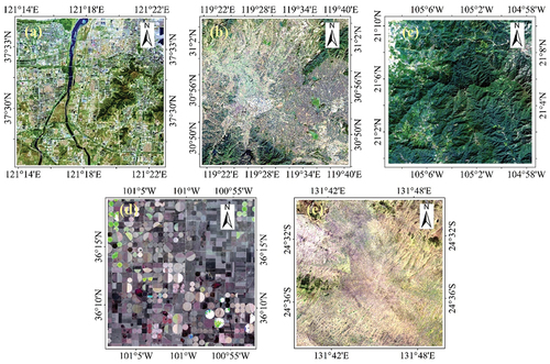
Five different sites were carefully selected for this cross-comparison: Yantai (Shandong, China), Xuancheng (Anhui, China), Rancho Viejo (Nayarit, Mexico), Ochiltree (Texas, USA), and the Gibson Desert (Australia) (Figure 1). The five sites represent completely different land surface types, allowing for a comprehensive assessment of the similarity between the two sensors’ data. Yantai was chosen due to its characteristic of densely developed built-up areas along with a few rivers. This site allows for assessing the similarity between the two satellite sensors in this built-up land-dominated area. Xuancheng features a mixture of built-up land, bare soil, farmland, and forest, making it suitable for evaluating consistency in both urban and country areas. Rancho Viejo is predominantly covered by forest and hence is used to evaluate the consistency in forested areas. Ochiltree is predominantly comprised of bare soil (fallow land) and a small amount of cultivated land and, therefore, is used mainly for examining the consistency in bare areas. The Gibson Desert site is characterized by red sand plains and rocky/gravelly ridges covered in thin desert grasses and thus is ideal for evaluating the consistency in desert areas. These test sites were chosen based on practical considerations rather than intentionally selecting homogeneous areas since real-world applications often lack homogeneity. Therefore, the evaluation conducted at these five test sites is expected to provide more practical insights into the performance and compatibility of the two satellite sensors.

Figure 1. Images of five test sites. (a) Yantai, China (175 km²); (b) Xuancheng, China (1185 km²); (c): Rancho Viejo, Mexico (397 km²); (d) Ochiltree, USA (547 km²); and (e) Gibson, Australia (298 km²).

The cross-comparison was conducted based on the data of the Collection 2 Level-2 product downloaded from the United States Geological Survey (USGS) website (https://earthexplorer.usgs.gov). The product includes both SR and LST data, which can be directly used without the need for further computation. This will ensure that the comparisons in this study are based on real USGS SR and LST data, avoiding the potential errors that could be introduced by manual calculations. Table 1 lists the underfly image pairs of Landsat-8 and −9 for the five test sites. It is worth noting that each image pair exhibits a very close time of overpass and nearly identical sun elevation and azimuth angles.

Table 1. Image pairs used for the study.

Image pair	Sensor	Path/Row	Acquisition date	Time of overpass (GMT)	Sun elevation angle (°)	Sun azimuth angle (°)	Area (km^2)
Yantai (China)	Landsat-8 OLI	119/34	14 November 2021	2:29:57	32.12	161.32	175
	Landsat-9 OLI2			2:32:13	32.09	161.19
Xuancheng (China)	Landsat-8 OLI	119/39	14 November 2021	2:31:56	38.41	157.88	1185
	Landsat-9 OLI2			2:34:13	38.37	157.75
Rancho Viejo (Mexico)	Landsat-8 OLI	30/45	14 November 2021	17:24:17	45.54	152.88	397
	Landsat-9 OLI2			17:24:34	45.48	152.74
Ochiltree (USA)	Landsat-8 OLI	30/35	14 November 2021	17:20:18	33.23	160.70	547
	Landsat-9 OLI2			17:20:36	33.20	160.57
Gibson (Australia)	Landsat-8 OLI	103/77	14 November 2021	01:07:56	64.43	80.92	298
	Landsat-9 OLI2			01:10:24	64.32	81.01

2.2. Comparison method

This study compared the SR and LST data of Landsat-8 and −9 in a three-level approach:

1. Band-level comparison: This is the first-level comparison. The corresponding bands of Landsat-8 and −9 were compared one by one to perform a band-by-band comparison. For the two thermal infrared bands, only band 10 was compared because band 11 of Landsat-8 has a larger bias and hence is not provided in the Collection 2 Level-2 product (Barsi et al. 2014; Cristóbal et al. 2018).

2. Indicator-level comparison: This serves as the second-level comparison, involving the calculation of the four indicators (Wetness, Greenness, Dryness, and Hotness) of the Remote Sensing based Ecological Index (RSEI).

Wetness indicator: The indicator is derived from a TCT wetness component, which reflects the moisture content in the environment. It helps in assessing water availability and detecting lands with high moisture. The equation for deriving the wetness component of Zhai et al. (2022) is expressed as:

(1) $\mathit{Wetness}=\mathit{\hspace{0.17em}}0.0382\mathit{Blue}+0.2137\mathit{Green}+0.3536\mathit{Red}+0.2270\mathit{NIR}-0.6108\mathit{MIR}1-0.6351\mathit{MIR}2$(1)

where Blue, Green, Red, NIR, MIR1, and MIR2 are the band names of Landsat-8/9 OLI/OLI2 sensor.

Greenness indicator: The indicator is represented by NDVI, which provides information about the presence and health of vegetation (S. Li et al. 2021). It is a measure of photosynthetic activity and can indicate the overall vegetation cover and vigor.

(2) $\mathit{NDVI}=\mathit{\hspace{0.17em}}(\mathit{NIR}-\mathit{Red})/(\mathit{NIR}+\mathit{Red})$(2)

Dryness indicator: This is represented by NDBSI (H. Q. Xu 2013), which provides information about the extent of built-up areas and bare soil. The indicator assists in identifying dry lands or low vegetation-cover areas and, therefore, is composed of the Index-based Built-up Index (IBI) (H. Xu 2008) and the Soil Index (SI) (Rikimaru, Roy, and Miyatake 2002):

(3) $\mathit{NDBSI}=\left(\mathit{IBI}+\mathit{SI}\right)/2$(3)

(4) $\mathit{IBI}=\{[2\mathit{MIR}1/(\mathit{MIR}1+\mathit{NIR})]-[\mathit{NIR}/(\mathit{NIR}+\mathit{Red})+\mathit{Green}/(\mathit{Green}+\mathit{MIR}1)]\}/\{[2\mathit{MIR}1/(\mathit{MIR}1+\mathit{NIR})]+[\mathit{NIR}/(\mathit{NIR}+\mathit{Red})+\mathit{Green}/(\mathit{Green}+\mathit{MIR}1)]\}$(4)

(5) $\mathit{SI}=\left[\left(\mathit{MIR}1+\mathit{Red}\right)-\left(\mathit{NIR}+\mathit{Blue}\right)\left]/\right[\left(\mathit{MIR}1+\mathit{Red}\right)\text{break}+\left(\mathit{NIR}+\mathit{Blue}\right)\right]$(5)

Hotness indicator: The indicator measures the land surface temperature (LST) of the Earth’s surface. It can provide insights into the thermal characteristics of different land cover types and identify areas with diverse temperatures. LST was obtained directly from band 10 of the Collection 2 Level-2 product, which has already been retrieved to LST by the USGS before being distributed.

The calculation of the above indicators involves utilizing almost all the bands from both Landsat-8 and Landsat-9 satellites. This comprehensive approach ensures that the bands from both satellites can be fully compared during the calculations.

• (3) Composite index-level comparison: This serves as the third-level comparison with RSEI computation. RSEI synthesizes the above four indicators through principal component analysis (PCA) and uses the first principal component (PC1) for synthesis.

RSEI is expressed as:

(6) $\mathit{RSEI}=\mathit{\hspace{0.17em}}\mathit{PC}1\left[\mathit{f}\left(\mathit{Wetness},\mathit{NDVI},\mathit{NDBSI},\mathit{LST}\right)\right]$(6)

RSEI values range from 0 to 1, with 0 representing the worst ecological status and 1 representing the best ecological status. Further information about RSEI can be found in the work of Xu et al. (2019). By calculating the PC1 of the four indicators, further comparison between the two satellite data can be achieved.

This study also conducts a comparative analysis of the consistency of the two satellite data in different land cover types, as inconsistency may vary with different land cover types. Based on the characteristics of the land cover types in the five test areas, six main land cover types were determined, which are forest, cropland, soil (fallow), barren (desert), built-up land, and water (river and lake). The method of visual interpretation was used to delineate the sample areas for each of the six land cover types from the five test sites. The sample sizes for each category are 655 for forest, 3544 for cropland, 4673 for soil, 1284 for barren, 1244 for built-up land, and 2506 for water. Based on these samples, the PC and R² values for the six land cover types were computed using the same three-level comparison method mentioned above.

2.3. Metrics to evaluate comparison

In statistical analysis, it is important to evaluate the deviation and correlation of two sets of data using appropriate indicators. When comparing two datasets, bias and its percent change (PC) can measure the difference between them but do not provide insights into the specific relationship between the datasets. R² is expressed as the square of the correlation coefficient (r) and thus can measure the strength of the relationship between two datasets (Kabir et al. 2023). However, R² does not account for the actual differences in values between the datasets. It’s worth noting that there is no definitive relationship between bias/PC and R². A small bias/PC value does not necessarily indicate a large R² value, and vice versa. For instance, consider the cases of y = x and y = 5x, both having an R² value of 1. However, the latter dataset exhibits a fivefold difference compared to the former. Therefore, if it is necessary to consider both the differences and the relationships between the datasets, a combination of indicators such as PC and R² can be employed for a comprehensive analysis.

Accordingly, the similarity between the data of the two satellites in this study was determined using Bias, PC, and R². The root mean square error (RMSE) was not used because both data ranges and units between the multispectral bands/indices and the thermal infrared band were not consistent.

The equations for Bias and PC are as follows:

(7) $\mathit{Bia}{s}_i=\mathit{mean}\left(\mathit{Landsat}-9_i\right)-\mathit{mean}\left(\mathit{Landsat}-8_i\right)$(7)

(8) $\begin{array}{rl}& \mathit{P}{C}_i=[\mathit{mean}\left(\mathit{Landsat}-9_i\right)-\mathit{mean}\left(\mathit{Landsat}-8_i\right)]/\mathit{abs}\\ & [\mathit{mean}\left(\mathit{Landsat}-8_i\right)]100\end{array}$(8)

where Bias_i and PC_i (%) are the bias and the percent change of the mean of band i or indicator i between Landsat-8 and −9, respectively.

R² is defined as:

(9) $R^2=r^2$(9)

(10) $\mathit{r}=\mathit{\hspace{0.17em}}(\mathrm{\Sigma }((\mathit{Landsat}-9_i-\mathit{\hspace{0.17em}}\mathit{mean}\left(\mathit{Landsat}-9\right))\ast (\mathit{Landsat}-8_i-\mathit{\hspace{0.17em}}\mathit{mean}\left(\mathit{Landsat}-8\right))))\mathit{\hspace{0.17em}}/(\surd (\mathrm{\Sigma }(\mathit{Landsat}-9_i-\mathit{\hspace{0.17em}}\mathit{mean}{\left(\mathit{Landsat}-9\right)}^2)\ast \surd (\mathrm{\Sigma }(\mathit{Landsat}-8_i-\mathit{\hspace{0.17em}}\mathit{mean}\left(\mathit{Landsat}-8\right){)}^2))$(10)

3. Results

3.1. First-level per-band comparison

Table 2 provides the results of the first-level per-band cross-comparison between the Landsat-8 OLI and Landsat-9 OLI2 bands across the five test sites. Metrics used to evaluate comparison results are Bias, PC, and R². The Bias is displayed with four decimal places to capture subtle differences that may only be observed at this level of precision.

Table 2. Statistics of the first-level per-band comparison.

	Band 1	Band 2	Band 3	Band 4	Band 5	Band 6	Band 7
Yantai
Bias	−0.0006	−0.0019	−0.0012	−0.0017	−0.0034	−0.0027	−0.0016
PC (%)	−1.03	−2.68	−1.30	−1.67	−1.94	−1.59	−1.21
R^2	0.807	0.888	0.934	0.941	0.957	0.961	0.958
Xuancheng
Bias	−0.0008	−0.0013	−0.0017	−0.0018	−0.0053	−0.0040	−0.0029
PC (%)	−1.81	−2.70	−2.54	−2.65	−2.32	−2.21	−2.58
R^2	0.863	0.930	0.965	0.973	0.970	0.968	0.966
Rancho Viejo
Bias	0.0008	−0.0005	0.0002	−0.0005	−0.0018	−0.0016	−0.0008
PC (%)	5.55	−2.64	0.60	−1.88	−0.60	−1.10	−1.14
R^2	0.808	0.918	0.976	0.985	0.975	0.983	0.989
Ochiltree
Bias	0.0003	−0.0004	0.0003	−0.0002	−0.0004	0.0003	−0.0002
PC (%)	0.457	−0.463	0.24	−0.12	−0.14	0.09	−0.07
R^2	0.928	0.964	0.976	0.986	0.993	0.987	0.993
Gibson
Bias	−0.0022	−0.0028	−0.0056	−0.0072	−0.0087	−0.0093	−0.0093
PC (%)	−5.23	−5.10	−5.57	−3.62	−3.05	−2.34	−2.63
R^2	0.544	0.813	0.961	0.944	0.957	0.945	0.942
Average bias	−0.0005	−0.0014	−0.0016	−0.0023	−0.0039	−0.0035	−0.0030
Average |PC| (%)	2.81	2.72	2.05	1.99	1.61	1.47	1.53
Average R^2	0.790	0.903	0.962	0.966	0.970	0.969	0.970

Spectrally, the two OLI sensors generally exhibit a high level of agreement over the five test sites. The average bias for each band ranges from −0.0039 to −0.0005, the average |PC| is less than 3%, and the average R² is greater than 0.9, except for band 1. However, the small negative biases averaging at −1.63% indicate a slightly lower reflectance for each band of Landsat-9 compared to the corresponding bands of Landsat-8. Among the seven multispectral bands, the coastal band (band 1) shows the highest deviations with the highest average |PC| value and the lowest average R² value. This was also found by Kabir et al. (2023).

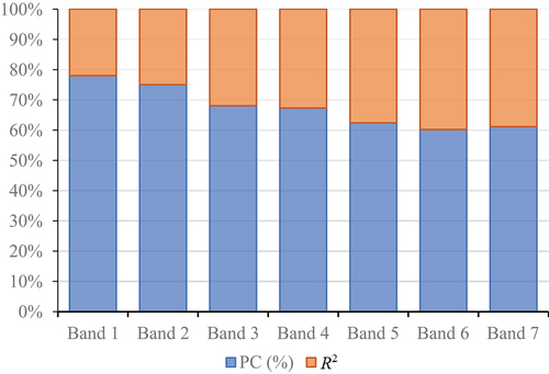
It is noted that the average |PC | decreases as the wavelength increases, dropping from 2.81% in band 1 to 1.47% in band 7 or from 2.21% to 1.25% if the Gibson desert site is excluded. On the other hand, the average R² value increases with longer wavelengths from 0.79 to 0.97, indicating an improvement in band consistency as the wavelength increases (Figure 2). This result is almost consistent with that of Gross et al. (2022), both in terms of the magnitude and pattern of the PC variation with wavelength. Badawi et al. (2019) have demonstrated that shorter wavelength bands in SR products had higher levels of uncertainty than the longer wavelength bands.

Figure 2. Percentage stacked bar chart illustrating the trends of average PC and R² as wavelength increases and a mutually inverse relationship between the two metrics.

3.2. Second-level indicator-based comparison

The indicator-level cross-comparison means that the comparison between the two satellite data is no longer conducted solely on a band-by-band basis. Instead, it involves comparing the results obtained after multiband calculations. The four indicators involved in this indicator-level comparison were Wetness, NDVI, NDBSI, and LST, which were calculated using Eqs (1(1) $\mathit{Wetness}=\mathit{\hspace{0.17em}}0.0382\mathit{Blue}+0.2137\mathit{Green}+0.3536\mathit{Red}+0.2270\mathit{NIR}-0.6108\mathit{MIR}1-0.6351\mathit{MIR}2$(1) –5(5) $\mathit{SI}=\left[\left(\mathit{MIR}1+\mathit{Red}\right)-\left(\mathit{NIR}+\mathit{Blue}\right)\left]/\right[\left(\mathit{MIR}1+\mathit{Red}\right)\text{break}+\left(\mathit{NIR}+\mathit{Blue}\right)\right]$(5) ). Based on the image pairs derived from the indicators, Table 3 provides the outcomes of the indicator-level comparison for the five test sites. The statistics of the four indicator-synthesized RSEI are also listed in this table for easy comparison with its indicators.

Table 3. Statistics of the second- and third-level comparisons.

	LST (^oC)	Wetness	NDVI	NDBSI	RSEI
Yantai
Bias	−0.5778	0.001	−0.0017	0.0013	0.0153
PC (%)	−3.34	1.01	−0.7	9.85	2.86
R^2	0.960	0.953	0.938	0.824	0.902
Xuancheng
Bias	−0.5394	0.0020	0.0005	0.0005	0.0252
PC (%)	−2.67	2.22	0.09	0.64	3.99
R^2	0.967	0.958	0.979	0.927	0.959
Rancho Viejo
Bias	−0.2696	0.0009	0.0020	−0.0028	−0.0104
PC (%)	−0.93	2.06	0.24	−1.04	−1.38
R^2	0.994	0.977	0.984	0.963	0.984
Ochiltree
Bias	−0.2232	−0.0002	−0.0002	0.0007	0.0007
PC (%)	−1.10	−0.09	−0.08	0.53	0.28
R^2	0.925	0.992	0.994	0.994	0.978
Gibson
Bias	0.4235	0.0058	0.0029	0.0035	0.0055
PC (%)	0.95	1.88	1.62	1.51	2.54
R^2	0.959	0.931	0.677	0.756	0.958
Average bias	−0.2373	0.0019	0.0007	0.0006	0.0073
Average |PC| (%)	1.80	1.45	0.55	2.71	2.21
Average R^2	0.961	0.962	0.914	0.893	0.956

The biases in Wetness, NDVI, and NDBSI are small, ranging from 0.0006 to 0.0019. The average |PC| values are below 2.71%, and average R² values exceed 0.893 (The LST will be discussed separately as it differs from these three indicators in data range and is not calculated using OLI’s multispectral bands but TIRS” thermal band).

NDBSI exhibits the largest average |PC| and the smallest average R², especially in the Yantai site, where built-up land is the predominant land cover type. The average |PC| approaches 10%, with the R² value of only 0.824. This indicates a greater deviation between the two satellites in NDBSI than in the other two indicators. Conversely, NDVI has the lowest average |PC| value, and Wetness falls in between. This seems to be related to the complexity of calculating these three indicators as well as the number of bands involved. Among these three indicators, NDBSI involves four bands and has the most complex calculation (Eqs 3(3) $\mathit{NDBSI}=\left(\mathit{IBI}+\mathit{SI}\right)/2$(3) -5(5) $\mathit{SI}=\left[\left(\mathit{MIR}1+\mathit{Red}\right)-\left(\mathit{NIR}+\mathit{Blue}\right)\left]/\right[\left(\mathit{MIR}1+\mathit{Red}\right)\text{break}+\left(\mathit{NIR}+\mathit{Blue}\right)\right]$(5) ). Wetness involves six bands but has a relatively straightforward computation (Eq 1(1) $\mathit{Wetness}=\mathit{\hspace{0.17em}}0.0382\mathit{Blue}+0.2137\mathit{Green}+0.3536\mathit{Red}+0.2270\mathit{NIR}-0.6108\mathit{MIR}1-0.6351\mathit{MIR}2$(1) ). NDVI, being the simplest, only utilizes two bands for its calculation (Eq 2(2) $\mathit{NDVI}=\mathit{\hspace{0.17em}}(\mathit{NIR}-\mathit{Red})/(\mathit{NIR}+\mathit{Red})$(2) ). In addition, according to the results of the first-level per-band comparison in Table 1, band 2 (blue band) has the second-largest average |PC| among the seven bands. Both NDBSI and Wetness calculations utilize this band, while NDVI does not involve it. This can also explain why NDVI has a lower average |PC| compared to NDBSI and Wetness.

Regarding LST, the bias metric indicates that the LST of Landsat-9 is on average −0.24°C lower than that of Landsat-8, with an average | PC | of 1.8% and an average R² of 0.961 across the five test areas. However, in the built-up land-dominated Yantai site, the LST of Landsat-9 can be −0.58°C lower than that of Landsat-8. Conversely, in the Gibson Desert site, it can be 0.42°C higher than that of Landsat-8.

Figure 3 showcases the density scatter plots of the four-indicator image pairs (Landsat-9 (L9) vs. Landsat-8 (L8)), the density scatter plots of bias as a function of Landsat-9 indicator values ((L9 vs. (L9 – L8)), and the histograms of the differencing images (L9 – L8). The scatter plots demonstrate a generally strong correlation between the indicator-image pairs of both satellites. The majority of scatter points for the Wetness, NDVI, and NDBSI indicators are closely clustered around the 1:1 line, indicating no clear visual indication of non-linearity. The dense point clouds of the differencing images (L9 vs. (L9 – L8)) of the three indicators align closely with the zero line. The histograms of the differencing images (L9 – L8) of the three indicators’ image pairs also show small deviations between the two satellites, as they have narrow distributions and near zero averages with Standard Deviation (SD) mostly smaller than 0.0421.

Figure 3. Indicator-based comparisons between Landsat-8 (L8) and Landsat-9 (L9) over the five test sites, with scatter plots of L9 vs. L8 (first row of each site), the density scatter plots of bias (L9 – L8) as a function of Landsat-9 indicator values (second row of each site), and the histograms of the differencing images (L9 – L8) (third row of each site).

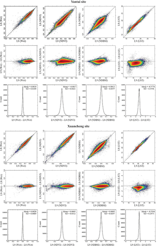
Figure 3. (Continued).

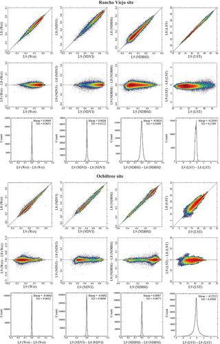
Figure 3. (Continued).

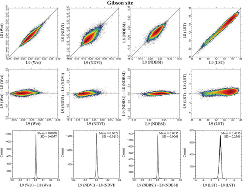
In terms of LST, since the LST of Landsat 9 is lower than that of Landsat 8 in the Yantai, Xuancheng, Rancho Viejo, and Ochiltree sites, the scatterplots of the three sites show that the LST data points located above the 1:1 line, while the scatterplot of (L9 LST) vs. (L9 LST – L8 LST) illustrates that scatter points appear mainly below the zero line. It can be observed that the LST of Landsat 9 is significantly lower than that of Landsat 8 primarily in its low- to mid-value range, especially in the Yantai and Xuancheng sites, where built-up land is a main land cover type. In the high-value range, the deviation between the two is relatively smaller. The histogram of the differencing images of the two satellites’ LSTs mostly exhibits a slightly left-skewed distribution. But in the Gibson Desert site, the LST of Landsat-9 is higher than that of Landsat-8, so its scatter plot and histogram behave exactly the opposite of the above-mentioned four test sites.

3.3. Third-level composite index-based comparison

The four indicators were integrated using Eq (6)(6) $\mathit{RSEI}=\mathit{\hspace{0.17em}}\mathit{PC}1\left[\mathit{f}\left(\mathit{Wetness},\mathit{NDVI},\mathit{NDBSI},\mathit{LST}\right)\right]$(6) to generate the composite index, RSEI. The statistics of the RSEIs across the five test sites are provided in Table 3. Figure 4 illustrates the results of this composite index-level comparison, including RSEI-image pairs, density scatter plots of the RSEI-image pairs (L9 vs. L8), density scatter plots by plotting biases against Landsat-9 RSEI values (L9 vs. (L9 – L8)), and histograms of the differencing images (L9 – L8).

Figure 4. Composite index (RSEI)-based comparison between Landsat-8 and Landsat-9 over the five test sites, with original true-color images (left of the first row of each site), RSEI image pairs (center and right of the first row of each site), scatter plots of L9 vs. L8 (left of the second row of each site), scatter plots of bias (L9 – L8) as a function of Landsat-9 values (center of the second row of each site), and histograms of the differencing images (L9 – L8) (right of the second row of each site).

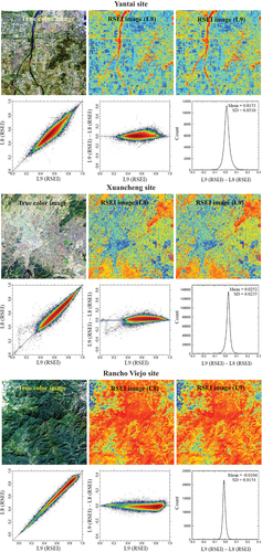
Figure 4. (Continued).

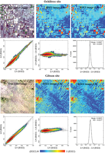
Figure 4 shows that the four-indicator-generated RSEI images of the two satellites are visually indistinguishable across the five test sites, with red tones representing good ecological status and blue tones representing poor ecological status. The figure demonstrates the strong agreement between the RSEI-image pairs of both satellites, with R² values ranging from 0.902 to 0.984 across the five sites (Table 3). Nevertheless, the statistics indicate that Landsat-9’s RSEI is slightly higher than Landsat-8’s RSEI on average by 0.0073 over the five sites, with an average |PC| value of 2.21% (Table 3). The majority of the points on the scatter plots spread closely along the 1:1 line, with a slight elevation above it. The dense points of the scatter plots of (L9 RSEI) vs. (L9 RSEI – L8 RSEI) align with the zero line but are slightly higher than the line, except for the Rancho Viejo site. This indicates a slightly higher value of RSEI for Landsat-9 compared to Landsat-8. The histograms of the differencing images of the two satellites” RSEI pairs show narrow distributions and near-zero averages with SDs mostly smaller than 0.03.

4. Discussion

4.1. Comparison among three levels

To examine the consistency in surface reflectance between Landsat-8 and −9 sensors, this study employed a three-level comparison, focusing on whether the differences in each band between the two satellites changed after subsequent calculations.

Table 4 presents the results of the three-level comparisons. The bias metric was not used for the comparison as the units and data ranges of measurement are not consistent across the three levels. To assess the actual differences and avoid cancellation between positive and negative values during accumulation, absolute values were used for the comparison. Additionally, since the calculation of RSEI did not involve the coastal band, the results of the first-level per-band comparison excluded the coastal band.

Table 4. Statistics of three-level comparisons.

	First level	Second level	Third level	Absolute average
Yantai
PC (%)	1.73	3.85	2.86	2.81
R^2	0.940	0.905	0.902	0.916
Xuancheng
PC (%)	2.50	0.98	3.99	2.49
R^2	0.962	0.955	0.959	0.959
Rancho Viejo
PC (%)	1.32	1.11	−1.38	1.27
R^2	0.971	0.975	0.984	0.977
Ochiltree
PC (%)	0.19	0.23	0.28	0.23
R^2	0.983	0.993	0.978	0.985
Gibson
PC (%)	3.72	1.65	2.54	2.64
R^2	0.927	0.788	0.958	0.891
Average |PC| (%)	1.88	1.63	2.21
Average R^2	0.957	0.933	0.956

In terms of the first-level per-band comparison, the two satellites exhibit a high level of consistency between their multispectral bands. This can be observed from the high average R² value (0.957) and the low average |PC | values (1.88%). The study by Kabir et al. (2023) showed that the median differences between Landsat-8 and −9 ranged from 1.5 to 2.5% for the visible bands.

The average |PC| increases from 1.88% in the first-level comparison to 2.21% in the third-level comparison, indicating an expansion of the deviation after the third-level operation. The R² value also slightly declines to 0.956 at the third level. The increased disparity in the third-level composite index-based comparison is probably due to the more complex calculation used to integrate the four indicators into RSEI through a relatively intricate principal component transformation. Although there is a slight reduction in average |PC| in the second-level comparison from 1.88% to 1.63%, the average R² value also significantly declines concurrently from 0.957 to 0.933, indicating a noticeable decrease in the correlation from the first-level to the second-level calculation.

4.2. Comparison among land cover types in the five test sites

Table 4 demonstrates that the comparative results of the five test sites are inconsistent. The lowest average R² value between Landsat-8 and −9 is observed in the Gibson desert site, with an average |PC| of 2.64% and an R² of only 0.891. The following sites in descending order are Yantai, Xuancheng, Rancho Viejo, and Ochiltree. Ochiltree has the lowest average |PC| of only 0.23% and the highest R² value of 0.985.

The reason for the different performances of the five test sites could be related to their land cover types. Therefore, this study further investigates the consistency between the two satellites across different land cover types. The major land cover types in the five test sites involved were forest, cropland, soil (fallow), barren (desert), built-up land, and water (river and lake). The statistical results of these six categories are presented in Table 5.

Table 5. Statistics of the six land cover types averaged across the five sites.

	Average |PC| of mean (%)			Average R^2
	Band level	Indicator level	Composite index level	Band level	Indicator level	Composite index level
Forest	2.15	1.14	1.24	0.805	0.914	0.933
Crop	1.70	0.97	1.85	0.904	0.958	0.967
Soil	1.15	0.97	3.57	0.879	0.781	0.739
Barren	3.75	1.72	2.62	0.769	0.598	0.699
Built-up	2.48	3.82	4.87	0.730	0.614	0.601
Water	18.62	34.02	15.47	0.521	0.560	0.160

Table 5 shows that among the six land cover types, the largest difference between Landsat-8 and −9 occurs in the water category. The average |PC| of the mean for this category reaches 18.62%, 34.02%, and 15.47% across the three comparison levels. The R² values are also the lowest among the six types, all being less than 0.6. Larger differences are also observed in the built-up land and barren categories. They show a notable decreasing trend for R² in the comparison from Level-1 to Level-3 comparison, with the average |PC| generally greater than approximately 2.5%. On the other hand, the vegetation-related categories (forest and cropland) exhibit better consistency, with differences generally smaller than 2% across the three levels and R² values mostly greater than 0.9. The different performances among the six land cover types reveal the reasons behind the greater disparity in reflectance data between the two satellites in Gibson, Yantai, and Xuancheng, as compared to Rancho Viejo and Ochiltree. This disparity can be attributed to the presence of more barren lands, built-up lands, or rivers/lakes in the former three sites.

4.3. Comparison of differences in radiometric resolution

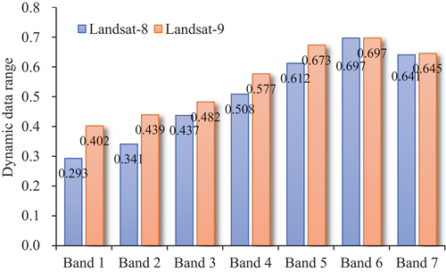
The Landsat-9 and Landsat-8 images have identical spatial resolution and band wavelength ranges but have differences in radiometric resolution. Landsat-9 has a higher radiometric resolution of 14 bits, while Landsat-8 is limited to 12 bits. Thus, it is expected that Landsat-9 should have a wider dynamic data range of each band compared to Landsat-8 as it can differentiate 16,384 shades compared to the 4096 shades of Landsat-8. Generally, high radiometric resolution can prevent saturation of reflectance in extremely bright or dark areas and reveal more details in regions with very bright or very dark characteristics, such as snow-covered or water areas (Rao, Garg, and Ghosh 2007; Yousuf et al., 2019). Therefore, it is necessary to examine whether the difference in radiometric resolution can cause variations in the reflectance data between the two satellites.

Figure 5 provides the dynamic data range of each band of the two OLI sensors averaged from the five test sites. The dynamic data range of each band was calculated by subtracting the minimum value from the maximum value of each band. The figure shows that the dynamic ranges of Landsat-9 bands are generally larger than those of Landsat-8, particularly in the visible to near-infrared bands. Therefore, the difference in data dynamic range caused by different radiometric resolutions is likely a reason behind the disparities in the reflectance data of the two satellites. The study by Kilic et al. (2016) also found that the radiometric resolution difference between Landsat-8 12-bit data and previous Landsat 8-bit data could yield an RMSE of around 1% when utilized for evapotranspiration calculations. Kabir et al. (2023) indicated that the signal-to-noise ratio of Landsat-9 was 7–30% higher than that of Landsat 8, which was likely attributable to its higher 14-bit radiometric resolution than Landsat-8’s 12-bit radiometric resolution.

Figure 5. Dynamic data range of each band of Landsat-8 and −9 averaged from the five test sites.

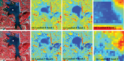
Due to the relatively large difference found in the water category, exceeding 15% across the three-level comparisons and even reaching up to 34%, we further investigated the reason that caused this notable discrepancy. Figure 6 provides the original Landsat-8 and −9 false-color images of a lake in the Xuancheng test site, as well as their pseudo-color images of bands 1 and 2. These images reveal that the two satellites exhibit significant differences in their ability to recognize the morphology of lake water in these two water-sensitive bands. It is evident that Landsat-9 outperforms Landsat-8 in identifying dark-colored water, as its identified area of dark-colored water (Figure 6f,g) is noticeably larger than that of Landsat-8 (Figure 6b,c). Clearly, the higher radiometric resolution of Landsat-9 enables it to distinguish dark-colored water effectively. When zoomed in on a specific area of dark water (white dot in Figure 6a), the lower radiometric resolution of Landsat-8 causes oversaturation in that area (Figure 6d), resulting in a large area appearing in a monotonous blue color. In contrast, Landsat-9 exhibits richer colors in the area where Landsat-8 appears oversaturated with blue color, effectively displaying the details of the dark water area (Figure 6h).

Figure 6. Images of a lake in the Xuancheng site, highlighting the radiometric solution difference in identifying dark water areas between Landsat-8 and −9. (a) and (e): Landsat-8 and −9 false-color images (RGB: bands 5, 4, 3); (b) and (c): Pseudo-color images of Landsat-8’s bands 1 and 2; (f) and (g): Pseudo-color images of Landsat-9’s bands 1 and 2; (d) and (h): Pseudo-color images with a zoomed-in view of the white dot in Figure 6(a,e).

4.4. Comparison between LST data

The thermal infrared sensor (TIRS) of Landsat-8 suffers from the problem of stray light incursion that contaminates the thermal image data collected from the instrument (Montanaro, Gerace, and Rohrbach 2015). One of the missions of Landsat-9 is to address this deficiency in Landsat-8. The TIRS-2 of Landsat-9 aims to significantly reduce the stray light to enable more precise LST measurements (Masek et al. 2020). Eon et al. (2023) validated Landsat-9 and Landsat-8 LST products and found the LST measurements of the two satellites agreed to be within 1 K over water and 2 K over sand. Their comparisons in the four lakes in Arizona showed that the LST of Landsat-9 was 0.21 K lower than that of Landsat-8 over the lakes in terms of the mean difference compared to in-situ measurements.

This comparison reveals that the LST measured by Landsat-9 is lower than that of Landsat-8 in the Yantai, Xuancheng, Rancho Viejo, and Ochiltree test sites. However, in the Gibson desert site, the LST of Landsat-9 is higher, resulting in an average difference of 0.24°C lower compared to Landsat-8 across all five sites (Table 2). In terms of the magnitude of the LST differences between the two satellites, Yantai, Xuancheng, and Gibson exhibit the largest disparities, with absolute biases ranging from 0.42 to 0.58°C. These three sites are primarily characterized by built-up lands or barren desert areas. In contrast, the Rancho Viejo and Ochiltree sites, which have minimal built-up land, show significantly smaller biases, averaging around 0.25°C. This suggests that the LST differences tend to be larger in barren desert areas and areas dominated by built-up land.

4.5. Limitations of this comparison

It should be noted that this study only used five test sites and included only six land cover types. Although these six land cover types encompass the major land cover types on the Earth’s surface, they still cannot represent all land cover types. The land cover types that are not included may have different performances. Additionally, the time period of this comparison was limited to mid-November only, and there is a lack of comparison for other seasons. This limitation primarily arises from the fact that this study strictly relies on underfly image data because the differences between the Landsat-8 and −9 data can be accurately compared only with precisely synchronized underfly image data. However, the underfly event was conducted only once in November 2021 and has not been carried out again. The lack of seasonally acquired underfly images makes it challenging to conduct a seasonal analysis. Therefore, this comparison does not capture differences between the two satellites across different seasons.

5. Conclusions

The recently launched Landsat-9 has been designed very closely to Landsat-8 for working together to reduce the revisit observation period of Landsat satellites to eight days. Therefore, ensuring the consistency of the data from both satellites is of utmost importance. This study used synchronized underfly image pairs of the two satellites from five test sites to evaluate the consistency of SR and LST data between the two by a three-level cross-comparison approach.

The first-level per-band comparison between the two satellites showed high consistency, with an average |PC| of 1.88% and an average R² of 0.957 across six bands in the five test sites. Small negative biases averaging at −1.63% found in this study indicate a slightly lower reflectance for each band of Landsat-9 compared to the corresponding bands of Landsat-8. However, there were higher deviations observed in the coastal and blue bands, with average | PC | values exceeding 2.8% and R² values lower than 0.85. There exists a trend of decreasing deviation with increasing wavelength.

The consistency between the two satellites decreases with increasing levels of comparison, indicated by the increase in the average |PC| values or the decrease in R² values across the five test sites. This three-level comparison approach suggests that the deviation found in the first-level comparison was amplified after complex computations. Nevertheless, the average |PC| is less than 2.5%, and R² is still higher than 0.95 at the third-level comparison.

Among the four indicators used to calculate RSEI, NDBSI has the largest difference between the two satellites, with an average R² of lower than 0.9 across the five test sites. Although the overall consistency of NDVI between the two satellites is relatively high, the low R² value of 0.68 in the Gibson desert site suggests that NDVI’s consistency is not high in sparsely vegetated desert areas. The comparison of LST data between both satellites reveals that the Landsat-9 LST is on average −0.24°C lower than Landsat-8 LST across the five test areas but can be 0.42°C higher in the Gibson desert area.

The land cover-based comparison has shown obvious disparities in the water category between the two satellites, with a high average | PC | between 15% and 35% and an average R² lower than 0.6. The built-up land and barren categories also have greater deviations compared to other categories. The differences in consistency among the land cover types have resulted in inconsistencies in the comparison results of the five test sites. Sites characterized by deserts or a high proportion of built-up land exhibit relatively lower consistency between the data from the two satellites.

This study demonstrates that despite no significant differences generally found in SR and LST data between Landsat-8 and −9, there can still be relatively large discrepancies occurring in certain bands and indices. These discrepancies are associated with the land cover types in the study area. Extra caution should be taken for areas characterized by deserts or containing significant amounts of water and/or built-up lands when both satellite data are used for time series analysis simultaneously.

Author contributions

H.Q.X. designed the study, carried out the data analysis, and wrote the original and revised drafts. R.M.J. processed the images. L.M.J. processed the images and revised the draft. ALL authors reviewed the manuscript.

Acknowledgments

We would like to thank the United States Geological Survey for providing the underfly images for this study. We would also like to express our gratitude to the four anonymous reviewers. Their valuable comments have greatly enhanced the quality of this paper.

Disclosure statement

No potential conflict of interest was reported by the author(s).

Data availability statement

The remote sensing image data utilized in this study can be obtained from the United States Geological Survey website (https://earthexplorer.usgs.gov). The other data are available from the corresponding author upon request.

Additional information

Funding

This work was supported by the National Natural Science Foundation of China [31971639] and the National Natural Science Foundation of Fujian Province, China [2023J01225].

References

- Angal, A., X. X. Xiong, and A. Shrestha. 2020. “Cross-Calibration of MODIS Reflective Solar Bands with Sentinel 2A/2B MSI Instruments.” IEEE Transactions on Geoscience and Remote Sensing 58 (7): 5000–19. https://doi.org/10.1109/TGRS.2020.2971462.
- Aurora, R. M., and K. Furuya. 2023. “Spatiotemporal Analysis of Urban Sprawl and Ecological Quality Study Case: Chiba Prefecture, Japan.” Land 12 (11): 2013. https://doi.org/10.3390/land12112013.
- Badawi, M., D. Helder, L. Leigh, and X. Jing. 2019. “Methods for Earth-Observing Satellite Surface Reflectance Validation.” Remote Sensing 11 (13): 1543. https://doi.org/10.3390/rs11131543.
- Barsi, J. A., J. R. Schott, S. J. Hook, N. G. Raqueno, B. L. Markham, and R. G. Radocinski. 2014. “Landsat-8 Thermal Infrared Sensor (TIRS) Vicarious Radiometric Calibration.” Remote Sensing 6 (11): 11607–11626. https://doi.org/10.3390/rs61111607.
- Chander, G., A. Angal, T. Choi, and X. Xiong. 2013. “Radiometric Cross-Calibration of EO-1 ALI with L7 ETM+ and Terra MODIS Sensors Using Near-Simultaneous Desert Observations.” IEEE Journal of Selected Topics in Applied Earth Observations and Remote Sensing 6 (2): 386–399. https://doi.org/10.1109/JSTARS.2013.2251999.
- Chander, G.; D. J. Meyer D. L. Helder. 2004. “Cross Calibration of the Landsat-7 ETM+ and EO-1 ALI Sensor.” IEEE Transactions on Geoscience & Remote Sensing 42 (12): 2821–2831. https://doi.org/10.1109/TGRS.2004.836387.
- Claverie, M., E. F. Vermote, B. Franch, and J. G. Masek. 2015. “Evaluation of the Landsat-5 TM and Landsat-7 ETM + Surface Reflectance Products.” Remote Sensing of Environment 169:390–403. https://doi.org/10.1016/j.rse.2015.08.030.
- Cristóbal, J., J. C. Jiménez-Muñoz, A. Prakash, C. Mattar, D. Skoković, and J. A. Sobrino. 2018. “An Improved Single-Channel Method to Retrieve Land Surface Temperature from the Landsat-8 Thermal Band.” Remote Sensing 10 (3): 431. https://doi.org/10.3390/rs10030431.
- Eon, R., A. Gerace, L. Falcon, E. Poole, T. Kleynhans, N. Raqueño, and T. Bauch. 2023. “Validation of Landsat-9 and Landsat-8 Surface Temperature and Reflectance During the Underfly Event.” Remote Sensing 15 (13): 3370. https://doi.org/10.3390/rs15133370.
- Farhad, M. M., M. Kaewmanee, L. Leigh, and D. Helder. 2020. “Radiometric Cross Calibration and Validation Using 4 Angle BRDF Model Between Landsat 8 and Sentinel 2A.” Remote Sensing 12 (5): 806. https://doi.org/10.3390/rs12050806.
- Firozjaei, M. K., M. Kiavarz, M. Homaee, J. Arsanjani, and S. Alavipanah. 2021. “A Novel Method to Quantify Urban Surface Ecological Poorness Zone: A Case Study of Several European Cities.” Science of the Total Environment 757:143755. https://doi.org/10.1016/j.scitotenv.2020.143755.
- Goward, S. N., P. E. Davis, D. Fleming, L. Miller, and J. R. G. Townshend. 2003. “Empirical Comparison of Landsat 7 and IKONOS Multispectral Measurements for Selected Earth Observation System (EOS) Validation Sites.” Remote Sensing of Environment 88 (1): 80–99. https://doi.org/10.1016/j.rse.2003.07.009.
- Gross, G., D. Helder, C. Begeman, L. Leigh, M. Kaewmanee, and R. Shah. 2022. “Initial Cross-Calibration of Landsat 8 and Landsat 9 Using the Simultaneous Underfly Event.” Remote Sensing 14 (10): 2418. https://doi.org/10.3390/rs14102418.
- Holden, C. E., and C. E. Woodcock. 2016. “An Analysis of Landsat 7 and Landsat 8 Underflight Data and the Implications for Time Series Investigations.” Remote Sensing of Environment 185:16–36. https://doi.org/10.1016/j.rse.2016.02.052.
- Hu, X. S., and H. Q. Xu. 2019. “A New Remote Sensing Index Based on the Pressure-State-Response Framework to Assess Regional Ecological Change.” Environmental Science and Pollution Research 26 (6): 5381–5393. https://doi.org/10.1007/s11356-018-3948-0.
- Ju, X. F., J. L. He, Q. Zhang, and S. Adilai. 2023. “Evolution Pattern and Driving Mechanism of Eco-Environmental Quality in Arid Oasis Belt — a Case Study of Oasis Core Area in Kashgar Delta.” Ecological Indicators 154:110866. https://doi.org/10.1016/j.ecolind.2023.110866.
- Kabir, S., N. Pahlevan, R. E. O’Shea, and B. B. Barnes. 2023. “Leveraging Landsat-8/-9 Underfly Observations to Evaluate Consistency in Reflectance Products Over Aquatic Environments.” Remote Sensing of Environment 296:113755. https://doi.org/10.1016/j.rse.2023.113755.
- Kaita, E., B. Markham, M. O. Haque, D. Dichmann, A. Gerace, L. Leigh, S. Good, M. Schmidt, and C. J. Crawford. 2022. “Landsat 9 Cross Calibration Under-Fly of Landsat 8: Planning, and Execution.” Remote Sensing 14 (21): 5414. https://doi.org/10.3390/rs14215414.
- Kamran, M., and K. Yamamoto. 2023. “Evolution and Use of Remote Sensing in Ecological Vulnerability Assessment: A Review.” Ecological Indicators 148:110099. https://doi.org/10.1016/j.ecolind.2023.110099.
- Kilic, A., R. Allen, R. Trezza, I. Ratcliffe, B. Kamble, C. Robison, and D. Ozturk. 2016. “Sensitivity of evapotranspiration retrievals from the METRIC processing algorithm to improved radiometric resolution of Landsat 8 thermal data and to calibration bias in Landsat 7 and 8 surface temperature.” Remote Sensing of Environment 185:198–209. https://doi.org/10.1016/j.rse.2016.07.011.
- Li, R., L. Wang, and Y. Lu. 2023. “A Comparative Study on Intra-Annual Classification of Invasive Saltcedar with Landsat 8 and Landsat 9.” International Journal of Remote Sensing 44 (6): 2093–2114. https://doi.org/10.1080/01431161.2023.2195573.
- Li, S., L. Xu, Y. Jing, H. Yin, X. Li, and X. Guan. 2021. “High-Quality Vegetation Index Product Generation: A Review of NDVI Time Series Reconstruction Techniques.” International Journal of Applied Earth Observation and Geoinformation 105:102640. https://doi.org/10.1016/j.jag.2021.102640.
- Masek, J. G., M. A. Wulder, B. Markham, J. McCorkel, C. J. Crawford, J. Storey, and D. T. Jenstrom. 2020. “Landsat 9: Empowering Open Science and Applications Through Continuity.” Remote Sensing of Environment 248:111968. https://doi.org/10.1016/j.rse.2020.111968.
- Metzler, M. D., and W. A. Malila, eds. 1985. “Characterization and Comparison of Landsat-4 and Landsat-5 Thematic Mapper Data.” Study of Spectral/Radiometric Characteristics of the Thematic Mapper for Land Use Applications, NASA Technical Report. Accessed February 14, 2024. https://ntrs.nasa.gov/api/citations/19860007220/downloads/19860007220.pdf
- Mishra, N., M. O. Haque, L. Leigh, D. Aaron, D. Helder, and B. Markham. 2014. “Radiometric Cross Calibration of Landsat 8 Operational Land Imager (OLI) and Landsat 7 Enhanced Thematic Mapper Plus (ETM+).” Remote Sensing 6 (12): 12619–12638. https://doi.org/10.3390/rs61212619.
- Montanaro, M., A. Gerace, and S. Rohrbach. 2015. “Toward an Operational Stray Light Correction for the Landsat 8 Thermal Infrared Sensor.” Applied Optics 54 (13): 3963–3978. https://doi.org/10.1364/AO.54.003963.
- Rao, N. R., P. K. Garg, and S. K. Ghosh. 2007. “Evaluation of Radiometric Resolution on Land Use/Land Cover Mapping in an Agricultural Area.” International Journal of Remote Sensing 28 (2): 443–450. https://doi.org/10.1080/01431160600733181.
- Rikimaru, A., P. S. Roy, and S. Miyatake. 2002. “Tropical Forest Cover Density Mapping.” Tropical Ecology 43 (1): 39–47.
- Tang, P. L., J. J. Huang, H. Zhou, C. L. Fang, Y. J. Zhang, and W. Huang. 2021. “Local and Telecoupling Coordination Degree Model of Urbanization and the Eco-Environment Based on RS and GIS: A Case Study in the Wuhan Urban Agglomeration.” Sustainable Cities and Society 75:103405. https://doi.org/10.1016/j.scs.2021.103405.
- Teillet, P. M., J. L. Barker, B. L. Markham, R. R. Irish, G. Fedosejevs, and J. C. Storey. 2001. “Radiometric Cross-Calibration of the Landsat-7 ETM+ and Landsat-5 TM Sensors Based on Tandem Data Sets.” Remote Sensing of Environment 78 (1): 39–54. https://doi.org/10.1016/S0034-4257(01)00248-6.
- Teillet, P. M., B. L. Markham, and R. R. Irish. 2006. “Landsat Cross-Calibration Based on Near Simultaneous Imaging of Common Ground Targets.” Remote Sensing of Environment 102 (3–4): 264–270. https://doi.org/10.1016/j.rse.2006.02.005.
- Thome, K. J., S. F. Biggar, and W. Wisniewski. 2003. “Cross Comparison of EO-1 Sensors and Other Earth Resources Sensors to Landsat-7 ETM+ Using Railroad Valley Playa.” IEEE Transactions on Geoscience and Remote Sensing 41 (6): 1180–1188. https://doi.org/10.1109/TGRS.2003.813210.
- Thome, K., J. D’Amico, and C. Hugon 2006. “Intercomparison of Terra ASTER, MISR, and MODIS, and Landsat-7 ETM+.” 2006 IEEE International Symposium on Geoscience and Remote Sensing, 1772–1775. Denver, CO, USA: 1-8.
- Voskanian, N., K. Thome, B. N. Wenny, M. H. Tahersima, and M. Yarahmadi. 2023. “Combining RadCalnet Sites for Radiometric Cross Calibration of Landsat 9 and Landsat 8 Operational Land Imagers (OLIs).” Remote Sensing 15 (24): 5752. https://doi.org/10.3390/rs15245752.
- Xu, H. 2008. “A New Index for Delineating Built‐Up Land Features in Satellite Imagery.” International Journal of Remote Sensing 29 (14): 4269–4276. https://doi.org/10.1080/01431160802039957.
- Xu, H. Q. 2013. “A Remote Sensing Urban Ecological Index and Its Application.” Acta Ecologica Sinica 33 (24): 7853–7862.
- Xu, H.-Q. 2015. “Retrieval of the Reflectance and Land Surface Temperature of the Newly-Launched Landsat 8 Satellite.” Chinese Journal of Geophysics 58 (3): 741–747.
- Xu, H. Q., S. L. Huang, and T. J. Zhang. 2013. “Built-Up Land Mapping Capabilities of the ASTER and Landsat ETM+ Sensors in Coastal Areas of Southeastern China.” Advances in Space Research 52 (8): 1437–1449. https://doi.org/10.1016/j.asr.2013.07.026.
- Xu, H. Q., Y. F. Wang, H. D. Guan, T. T. Shi, and X. S. Hu. 2019. “Detecting Ecological Changes with a Remote Sensing Based Ecological Index (RSEI) Produced Time Series and Change Vector Analysis.” Remote Sensing 11 (20): 2345. https://doi.org/10.3390/rs11202345.
- Xu, H. Q., M. Y. Wang, T. T. Shi, H. D. Guan, C. Y. Fang, and Z. L. Lin. 2018. “Prediction of Ecological Effects of Potential Population and Impervious Surface Increases Using a Remote Sensing Based Ecological Index (RSEI).” Ecological Indicators 93:730–740. https://doi.org/10.1016/j.ecolind.2018.05.055.
- Xu, G. Z., and H. Q. Xu. 2021. “Cross-Comparison of Sentinel-2A MSI and Landsat 8 OLI Multispectral Information.” Remote Sensing Technology and Application 36 (1): 165–175.
- Xu, H. Q., and T. Zhang. 2013. “Assessment of Consistency in Forest-Dominated Vegetation Observations Between ASTER and Landsat ETM+ Images in Subtropical Coastal Areas of Southeastern China.” Agricultural and Forest Meteorology 168:1–9. https://doi.org/10.1016/j.agrformet.2012.08.012.
- Ye, X., H. Z. Ren, Y. Z. Liang, J. Zhu, J. Guo, J. Nie, H. Zeng, Y. H. Zhao, and Y. Qian. 2021. “Cross-Calibration of Chinese Gaofen-5 Thermal Infrared Images and Its Improvement on Land Surface Temperature Retrieval.” International Journal of Applied Earth Observation and Geoinformation 101:102357. https://doi.org/10.1016/j.jag.2021.102357.
- Yousuf, B., A. Shukla, M. K. Arora, and A. S. Jasrotia. 2019. “Glacier Facies Characterization Using Optical Satellite Data: Impacts of Radiometric Resolution, Seasonality, and Surface Morphology.” Progress in Physical Geography: Earth and Environment 43 (4): 473–495. https://doi.org/10.1177/0309133319840770.
- Zhai, Y., D. P. Roy, V. S. Martins, H. Zhang, L. Yan, and Z. Li. 2022. “Conterminous United States Landsat-8 Top of Atmosphere and Surface Reflectance Tasseled Cap Transformation Coefficients.” Remote Sensing of Environment 274:112992. https://doi.org/10.1016/j.rse.2022.112992.
- Zhou, D. C., L. X. Zhang, H. Lin, J. Fan, Y. Li, and H. Y. Zhang. 2023. “Satellite Evidence for Small Biophysical Effects of Transport Infrastructure in the Qinghai-Tibet Plateau.” Journal of Cleaner Production 416:138002. https://doi.org/10.1016/j.jclepro.2023.138002.