Remote sensing of terrestrial gross primary productivity: a review of advances in theoretical foundation, key parameters and methods

ABSTRACT

Accurately estimating gross primary productivity (GPP), the largest carbon flux in terrestrial ecosystems, is crucial for advancing our understanding of global carbon cycle and predicting climate feedbacks. The advancements in remote sensing (RS) have facilitated the development of GPP estimation models at regional and global scales in recent decades. This article systemically reviews the development of RS-based GPP estimation in three main aspects: theoretical foundation, key parameters and methods. Regarding the theoretical foundation, RS generally excels in representing key characteristics during the light transmission process of photosynthesis. However, it exhibits a relatively weaker ability to describe the carbon reaction process, severely limiting the in-depth understanding of the mechanisms of RS-based GPP estimation. Concerning key parameters, the definition of traditional parameters, such as leaf area index (LAI), photosynthetically active radiation (PAR), and fraction of absorbing PAR, has been detailed in the development of RS (e.g. LAI is divided into sunlit LAI and shaded LAI). However, their accuracy still needs improvement. Additionally, researchers have developed effective parameters (e.g. photochemical reflectance index, sun-induced chlorophyll fluorescence, and the maximum carboxylation rate) that possess increased capability to represent and interpret the carbon reaction process of photosynthesis. Regarding estimation methods, although the four main categories of RS-based GPP estimation models (statistical model, light use efficiency model, RS-based process model and machine learning-based model) have made significant progress in parameter optimization, the estimation accuracy and mechanism innovation remain less than satisfactory. Finally, we summarize the current issues of RS-based GPP estimation related to parameters performance and accuracy, model mechanisms and capabilities, as well as scale and connotation mismatch. Integrating more adequate in situ and comprehensive observations would enhance the interpretability of GPP estimation models, providing more reliable insights into the mechanisms in future studies. This article contributes to understanding of the photosynthetic process and RS-based GPP estimation, potentially aiding in the development of parameter optimization (improving the estimation accuracy of existing parameters and developing new ones) and model design (introducing new parameters and exploring new mechanistic models).

KEYWORDS:

• Gross primary production (GPP)
• light use efficiency (LUE)
• photosynthetic process
• remote sensing
• sun-induced chlorophyll fluorescence (SIF)

1. Introduction

Gross primary productivity (GPP) constitutes the principal carbon cycle flux in terrestrial ecosystems, encompassing all carbon dioxide (CO₂) absorbed by vegetation from the atmosphere via photosynthesis (Beer et al. 2010; Chapin et al. 2006; Ryu, Berry, and Baldocchi 2019; Xiao, Jin, and Dong 2014). Accurate GPP estimation serves as the foundation for comprehending the carbon budget, climate change, and ecosystem services (Anav et al. 2015; Beer et al. 2010; Xia et al. 2015; Zhang et al. 2019).

Researchers have made significant strides in quantifying terrestrial GPP at regional and global scales, despite the inherent challenges in directly measuring GPP (Welp et al. 2011). In terms of ground observations, techniques related to eddy covariance (EC) provide a dependable indirect approach for measuring GPP at the ecosystem scale. Presently, hundreds of flux sites, encompassing diverse global vegetation types, have undergone standardized processing and assessment of their records (Pastorello et al. 2020). The existence of EC GPP data, with a spatial scale (footprint) comparable to satellite pixels, facilitates the implementation of vegetation GPP monitoring. EC GPP data serve not only as the benchmark for validating satellite-based GPP estimation but are also as a convenient tool for model optimization, including parameters and structures. Furthermore, in satellite observations, the advancement of visible, synthetic aperture radar (SAR), light detection and ranging (Lidar), and notably, sun-induced chlorophyll fluorescence (SIF) remote sensing, enables the estimation of various plant parameters closely linked to photosynthesis using remote sensing (RS) methods. Capitalizing on the advantages of RS, including large-scale synchronous observation and fine temporal and spatial resolution, RS-based methods prove to be relatively more efficient in exploring the dynamic of GPP and its spatiotemporal variations at the regional scale (Sun et al. 2019; Yuan et al. 2014). RS-based methods are comparatively simpler when juxtaposed with process-oriented ecosystem models, which typically require a substantial set of input parameters (Pei et al. 2022; Piao et al. 2013). Consequently, RS-based GPP estimation methods have undergone rapid development over the past few decades.

In recent decades, our understanding of photosynthesis in terrestrial ecosystems has deepened and become more multidimensional (Beer et al. 2010; Ryu, Berry, and Baldocchi 2019; Schimel et al. 2019; Sellers et al. 1997) through the continuous development and integrated application of biochemistry, plant physiology ecology, and RS. These advancements contribute to the progress of multiscale terrestrial GPP estimation models. Over time, the increasing number of RS-based GPP estimation methods can be categorized into statistical models, parametric models, RS-related process models, machine learning approaches and proxy methods (Xiao et al. 2019). Meanwhile, several recent studies have reviewed the development of RS-based GPP estimation in terrestrial ecosystems from various perspectives (Liang and Wang 2020; Liao et al. 2023; Pei et al. 2022; Ryu, Berry, and Baldocchi 2019; Siebers et al. 2021; Song, Dannenberg, and Hwang 2013; Sun et al. 2019; Xiao et al. 2019). For example, Ryu et al. (2019) reviewed the history of quantifying global terrestrial photosynthesis, analyzing uncertainties and identifying opportunities. Xiao et al. (2019) summarized the evolution of RS-based measures for monitoring carbon flux and storage over the last 50 years, providing detailed elaborations on platforms, sensors, methods, breakthroughs, and challenges. Siebers et al. (2021) explored the development of cross-scale methods, from leaf to canopy scale, for measuring vegetation photosynthesis from the perspectives of RS and gas exchange. Pei et al. (2022) reviewed the evolution of parameters in light use efficiency (LUE) models, analyzed the uncertainties arising from different parameters, and offered new insights for optimizing the LUE model.

Existing reviews predominantly concentrate on analyzing the progress of RS-based GPP estimation methods, yet they lack sufficient discussion on the theoretical foundation and key parameters of these methods. Consequently, this study aims to systematically review the development of RS-based GPP estimation, covering three main aspects: theoretical foundation, key parameters, and methods. This endeavor seeks to offer a comprehensive understanding of the current development status, progressing from theory to parameters and subsequently to models. Initially, we provide a concise summary of the plant photosynthetic process and the theory behind RS-based GPP estimation. Subsequently, we elucidate the progression of RS parameters closely associated with the photosynthetic process and review the evolving pathways of four categories of GPP estimation models. Lastly, we enumerate the issues and challenges in RS-based GPP estimation, offering novel insights for future research.

2. Theory of satellite based GPP monitoring

2.1. Photosynthesis process

Photosynthesis constitutes a complex biochemical process. Prior research has furnished an elaborate summary of plant photosynthesis (Jones 2014; Kiang et al. 2007; Lambers, Chapin, and Pons 2008; Porcar-Castell et al. 2014). In this context, we elucidate the photosynthetic process from the standpoint of remote sensing, with primarily referring to the work of Porcar-Castell et al. (2014). This involves simplifying the entire process into the light transmission stage and carbon reaction stage, according to the timing of SIF emission (Figure 1).

Figure 1. The theoretical foundation of remotely sensed GPP estimation. Photosynthesis process at leaf scale was referenced from Porcar-Castell et al. (2014) and Patel et al. (2018), and remote sensing monitoring was referenced from Thenkabail et al. (2011). LAI: leaf area index; CI: clumping index; FVC: fractional vegetation cover; Ta: air temperature; VPD: vapor pressure deficit; LST: land surface temperature; SM: soil moisture; PAR: photosynthetically active radiation; APAR: absorbed photosynthetically active radiation; LUE: light use efficiency; SIF: solar-induced chlorophyll fluorescence; [N]: nitrogen content; [cab]: chlorophyll concentration; NADPH: nicotinamide adenine dinucleotide phosphate; ATP: Adenosine triphosphate; H⁺: electrons generated by water splitting; J_max: maximum electron transport rate (μmol m⁻² s⁻¹); V_cmax: maximum carboxylation rate (μmol m⁻² s⁻¹); GPP: gross primary production. See more symbols and acronyms in Appendix A.

In the light transmission stage, photosynthetically active radiation (PAR) that reaches the leaves is partially reflected and absorbed, while the remainder traverses through the canopy. Only the PAR absorbed by photosynthetic pigments (APAR_chl) is utilized for photosynthesis, whereas the light absorbed by nonphotosynthetic pigments does not directly contribute to the photosynthesis process. In other words, chlorophyll concentration determines the APAR. The APAR_chl undergoes three distinct transformations during the photosynthetic process (Baker 2008; Maxwell and Johnson 2000; Porcar-Castell et al. 2014): (1) further contribution to photosynthesis, driving the carbon reaction process; (2) heat dissipation (nonphotochemical quenching, NPQ), a byproduct of the xanthophyll cycle, is more pronounced when the photosynthetic rate decreases under environmental stresses; and (3) SIF, electromagnetic radiation emitted by plants during daylight in the red and near-infrared wavelengths (650–850 nm), is also a byproduct of photosynthesis. These three components exhibit a competitive relationship under normal conditions, signifying that an increase in one results in a decrease in the other two (Maxwell and Johnson 2000). The canopy structure can impact photosynthesis at the canopy scale. In other words, factors such as leaf area index (LAI), clumping index (CI), and fraction of vegetation cover (FVC), among others, can influence the APAR.

In the carbon reaction stage, electrons separated from H₂O driven by APAR are transported to NADP+, converting it to nicotinamide adenine dinucleotide phosphate (NADPH). Concurrently, adenosine triphosphate (ATP) is generated from adenosine diphosphate (ADP) through phosphorylation driven by the electron transport chain (Kaiser et al. 2015; Mohammad Mahdi and Babak 2012; Porcar-Castell et al. 2014). The maximum electron transport rate (J_max) serves as the pivotal variable influencing the aforementioned reaction process (Long and Bernacchi 2003). Subsequently, CO₂ is converted to carbohydrates through ATP and NADPH under the catalytic effect of the Rubisco enzyme, and the maximum carboxylation rate (V_cmax) stands out as the crucial variable in this process (Farquhar, von Caemmerer, and Berry 1980; Long and Bernacchi 2003; Walker et al. 2014).

At the leaf scale, nitrogen, chlorophyll, and leaf water play crucial roles in photosynthesis, serving as carriers and raw materials for photosynthesis (Evans 1989). Furthermore, environmental conditions such as PAR, temperature, and water, can impact the overall conversion process by modifying stomatal states or restricting enzyme activity (Ahmad et al. 2023).

2.2. Satellite based GPP estimation

RS primarily derives information from the reflectance at various wavelengths and the emission of SIF. The reflectance at specific wavelengths reveals distinct characteristics of the vegetation (Figure 1). For example, the reflectance at visible wavelengths is closely linked to chlorophyll content (Rouse 1974), and that at 531 nm is associated with xanthophyll content (Gamon, Serrano, and Surfus 1997). Additionally, the reflectance at 650–800 nm correlates with SIF (Meroni et al. 2009), and that in the short-wave infrared (SWIR) range is related to water content (Fang et al. 2017; Sims and Gamon 2003). Key parameters (e.g. LAI and FPAR) related to the photosynthetic process can be derived from the reflectance at each specific wavelength.

Photosynthesis at the ecosystems scale of is referred to as GPP (Chapin, Matson, and Vitousek 2011). Remotely sensed GPP is an approximate estimation using one or more remotely sensed indicators or parameters related to the photosynthetic process (often simplified). Remotely sensed GPP estimation models consist of various parameters representing plant status (including morphological, physiological and biochemical characteristics) and environmental conditions. The models are based on the simplification of the real photosynthetic process and some special assumptions.

Importantly, the majority of current RS-based parameters (especially reflectance-based parameters; e.g. LAI and FPAR) are still inadequate to characterize the photosynthetic process (especially for the carbon reaction) and cannot accurately quantify actual photosynthesis (Zhang et al. 2014). Consequently, most RS-based estimates could be regarded as an approximation of potential GPP rather than realized GPP.

In Figure 1, the vegetation spectral features directly detectable for remote sensing are primarily concentrated in the light transmission stage. In contrast, information from the carbon reaction stage cannot directly reach remote sensing sensors. Consequently, remote sensing measures excel in characterizing key features of the light transmission stage but demonstrate a relatively weak ability to characterize features of the carbon reaction stage.

3. Key parameters in remotely sensed GPP estimation

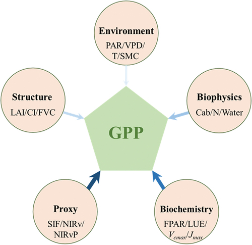
Based on the theoretical foundation of GPP estimation (Figure 1), we have summarized five key parameters (Figure 2) obtainable from RS that are closely linked to the photosynthetic process in terrestrial ecosystems. While some parameters have not been utilized in existing GPP estimation, we believe they hold significance for accurate GPP estimation. These include: (1) structure parameters, such as LAI, CI, FVC and canopy stomatal conductance; (2) biophysical parameters, such as chlorophyll concentration, nitrogen content and leaf water content; (3) biochemical parameters, such as FPAR, LUE, V_cmax and J_max; (4) proxy indicators, such as the byproduct of photosynthesis (e.g. SIF) and its proxies (e.g. NIR_V (near-infrared reflectance of terrestrial vegetation; NIR × NDVI) and NIR_VP (NIR_V × PAR)); and (5) photosynthesis-related environmental parameters, such as PAR, land surface temperature (LST), soil moisture content (SMC) and vapor pressure deficit (VPD).

Figure 2. Five key parameters closely linked to the photosynthetic process. The size and color of the arrows depict the degree of correlation between these parameters and remotely sensed GPP estimation. See more symbols and acronyms in Appendix A.

Several studies have provided comprehensive reviews of their development; for example, Fang et al. (2019) reviewed the LAI, Tao et al. (2020) reviewed the FPAR, and Mohammed et al. (2019) reviewed the SIF. Consequently, in this section, our main emphasis is on the advancement of remotely sensed inversion techniques for biochemical parameters.

3.1. Vegetation structure parameters

Vegetation structure parameters encapsulate three-dimensional information to some extent, influencing the absorption of solar light within the canopy and subsequently modifying the amount of absorbed energy to leaves. Furthermore, the structure parameter is a pivotal variable for remotely sensed GPP estimation at the canopy scale and serves as a link to facilitate the conversion of scales between canopy and leaf. The key vegetation structure parameters encompass LAI, CI, FVC and canopy stomatal conductance.

LAI stands out as one of the most widely utilized structure parameters in remotely sensed GPP estimation, serving as a direct or indirect input variable in different models. LAI is generally defined as one half of the total green leaf area per unit horizontal ground surface area (Chen and Black 1992). Significantly, LAI is further categorized into LAI_sun (sunlit LAI) and LAI_shade (shaded LAI) at the canopy level (Chen, Chen, and Ju 2007; Chen et al. 2012). RS-based estimation of LAI has undergone extensive exploration over the past few decades, resulting in the generation of various LAI products (Chen 2018; Fang et al. 2019). However, concerted efforts are needed to advance LAI estimation algorithms, offering higher temporal and spatial resolution, as well as the spatial continuity products (Fang et al. 2019).

CI emerges as a crucial structure parameter delineating the spatial pattern of canopy leaf distribution (clump, random, regular, etc.). Technically, CI is defined as the ratio of the effective LAI (LAI_e, (Chen, Menges, and Leblanc 2005)) to the real LAI (Chen 2018; Chen, Menges, and Leblanc 2005; Nilson 1971), i.e. CI = LAI_e/LAI. RS-based CI products predominantly rely on empirical relationship with normalized difference hotspot and darkspot index; future studies should explore physical retrieval methods to obtain high-resolution CI (Fang 2021). In addition, the estimation of FVC is grounded in scaled maximum/minimum VI values, with key challenges lying in determining the appropriate VI values for full vegetation cover and bare soil (Gao et al. 2020). Similarly, stomatal conductance is typically calculated based on VI (Yebra et al. 2013), LAI (Yan et al. 2012) or specific models (Wang and Leuning 1998).

3.2. Vegetation biophysical parameters

Chlorophyll, nitrogen and leaf water are pivotal components of vegetation photosynthesis, and their content or concentration represents the potential ability of photosynthesis. Additionally, specific RS indices based on specific wavelengths play a role in characterizing these features.

Chlorophyll concentration (Finegan et al. 2015) is closely related to the photosynthetic capability (Gitelson et al. 2006, 2014). Researchers have developed numerous chlorophyll-related indices based on the “red edge” wavelengths (680–760 nm) that are sensitive to variations in Cab, especially those near 700 nm (Zhang et al. 2022). Numerous studies have evidenced the close relationship between nitrogen content and Cab (Berger et al. 2020), indicating that remotely sensed chlorophyll-related indices serve as a proxy for nitrogen content (Homolová et al. 2013). Currently, parametric regressions, radiative transfer modeling and machine learning-based approaches are the most widely adopted methods for nitrogen monitoring (Berger et al. 2020).

The remotely sensed estimation of leaf water content, also referred to as equivalent water thickness (EWT), represents the water content per unit leaf area (Yilmaz, Hunt, and Jackson 2008). The remotely sensed monitoring of leaf water content primarily employs indices (Fang et al. 2017; Sims and Gamon 2003) constructed using reflectance wavelengths related to vegetation water content (i.e. near-infrared (NIR) and SWIR). Additionally, vegetation optical depth (VOD) measures the attenuation of microwave radiation caused by vegetation and thus correlates with total vegetation water content (Jackson and Schmugge 1991). VOD can be retrieved from both passive and active microwave data, with numerous estimation models and productions of VOD available at L (1–2 GHz), C (4–8 GHz), X (8–12 GHz), and K (18–26.5 GHz) bands (Frappart et al. 2020). In recent years, studies have proposed using VOD to estimate GPP (Dou et al. 2023; Teubner et al. 2019).

3.3. Vegetation biochemical parameters

The vegetation biochemical parameter is crucial for characterizing the absorption and conversion of energy during the photosynthetic process, directly influencing GPP. In this section, we illustrated the development of some key biochemical parameters, namely, FPAR, LUE and V_cmax.

3.3.1. Fpar

FPAR is defined as the fraction of absorbed PAR to incident PAR (solar light within 400–700 nm), directly representing the capability to intercept and absorb solar energy. FPAR serves as the core parameter, indicating the absorbed PAR of all plant organs, encompassing both the photosynthetically active portion (PAV) and the non-photosynthetically active portion of the vegetation (NPV) (Goward and Huemmrich 1992; Xiao et al. 2004). The interpretation of remotely sensed FPAR estimation has become more comprehensive and specific, including canopy-scale FPAR (FPAR_canopy, (Goward and Huemmrich 1992)), leaf-scale FPAR (FPAR_foliage, (Braswell et al. 1996)), green leaf-scale FPAR (FPAR_green, (Hall et al. 1992)), and chlorophyll-scale FPAR (FPAR_chl, (Zhang et al. 2005)). Theoretically, the order of these four parameters, in terms of magnitude, would be FPAR_canopy > FPAR_foliage > FPAR_green > FPAR_chl. Additionally, Xiao et al. (2004) considered the FPAR of PAV (FPAR_PAV, also called FPAR_foliage or FPAR_green) as the only effective part for photosynthesis; He et al. (2013) divided the total FPAR into sun leaves FPAR (FPAR_sun) and shade leaves FPAR (FPAR_shade). Currently, empirical methods and radiative transfer models are most commonly used approaches in RS-based FPAR estimation (Tan et al. 2013; Tao, Xiao, and Fan 2020). Notably, cloud contamination remains the primary influencing factor in most optical satellite-based FPAR estimations. Therefore, microwave RS, which avoids the influence of clouds, provides a new approach for remotely sensed FPAR estimation (Wang et al. 2021).

3.3.2. Lue

LUE represents the efficiency of converting absorbed energy into organic carbon and serves as a core parameter in remotely sensed GPP estimation models, particularly in the LUE model. To date, LUE estimation has become more detailed. For example, Zhang et al. (2009) provided redefinitions for LUE_chl and LUE_canopy according to FPAR_chl and FPAR_canopy; He et al. (2013) further categorized the LUE into sunlit LUE (LUE_sun) and shaded LUE (LUE_shade).

RS can indirectly quantify LUE through the NPQ generated during the photosynthesis process (Damm et al. 2010). The photochemical reflectance index (PRI), utilizing the narrow reflectance wavelengths at 531 nm and 570 nm (PRI = (ρ531 – ρ570)/(ρ531 + ρ570)), effectively characterizes xanthophyll cycle variation, linked to NPQ (Gamon, Peñuelas, and Field 1992). Numerous studies have shown the close connection between PRI and LUE (Barton and North 2001; Filella et al. 1996; Gamon, Serrano, and Surfus 1997; Garbulsky et al. 2011). Rahman et al. (2004) extrapolated this relationship from leaf to canopy scale and utilized it (calculated with the moderate resolution imaging spectroradiometer (MODIS) bands 11 and 12) as a proxy for LUE in GPP estimation. Subsequent investigations explored the PRI-LUE relationship using different satellite sources, including MODIS (Drolet et al. 2005, 2008; Goerner, Reichstein, and Rambal 2009; Guarini et al. 2014; Hall, Hilker, and Coops 2011; Middleton et al. 2016; Moreno et al. 2012; Ulsig et al. 2017), CHRIS/PROBA hyperspectral (Hilker et al. 2011; Stagakis et al. 2014), and Hyperion/EO-1 hyperspectral (Hernández-Clemente et al. 2016). Indices derived from PRI are also employed to estimate LUE (Nakaji et al. 2007; Rossini et al. 2010). Additionally, SIF is utilized for LUE estimation. Damm et al. (2010) demonstrated that SIF’s sufficiency as a proxy for LUE and its enhanced performance when combined with PRI (Cheng et al. 2013), leading to significantly improved GPP estimation accuracy. Similar findings are reported by Kováč et al. (2022), enhancing the GPP estimation model performance in both evergreen and deciduous forests using a combination of normalized difference vegetation index (NDVI, see calculation in Appendix B), PRI and SIF.

3.3.3. V_cmax and J_max

The maximum carboxylation rate (V_cmax) and the maximum electron transport rate (J_max) are key parameters in most models that characterize the interaction of carbon, energy and moisture between land and atmosphere. A robust correlation exists between V_cmax and J_max (Alton 2017; Beerling and Quick 1995; Domingues et al. 2010; Walker et al. 2014). For example, Walker et al. (2014) established a linear relationship between ln(V_cmax) and ln(J_max). Additionally, recent studies have validated the calculation of leaf-scale V_cmax using reflectance data (Dillen et al. 2012; Serbin et al. 2012, 2015). These studies typically utilize near-ground reflectance observations (e.g. 400–2500 nm) and establish the relationship between reflectance and V_cmax through partial least squares regression (PLSR). Serbin et al. (2015) also illustrated the close relationship between V_cmax and visible (400–700 nm), NIR (1150–1300 nm) and SWIR (1300–2500 nm). Furthermore, Fu et al. (2020) demonstrated that reflectance data within 400–900 nm (as predicting factors) can delineate a spatial pattern of canopy-scale V_cmax and J_max using a dataset based on a hyperspectral camera.

Concurrently, researchers have identified a strong linear or nonlinear relationship between V_cmax and the vegetation index (e.g. NDVI and enhanced vegetation index (EVI)) when accounting for seasonal variation in plants (i.e. dividing the growing season into two stages according to the DOY of the peak) (Muraoka et al. 2013; Zhou et al. 2014). At the canopy scale, Alton (2017) estimated the V_cmax of the top canopy using the MODIS LAI and the medium resolution imaging spectrometer (MERIS) terrestrial chlorophyll index (MTCI) (V_cmax ∼ MTCI/f (LAI)) and reported the linear relationship between J_max and chlorophyll (J_max = a f (MTCI) + b); these findings have since been globally applied (Alton 2018).

The GPP observations of flux towers also provide a method to estimate V_cmax. Zheng et al. (2017) developed a method that combines eddy-covariance observations and photo response curves to derive V_cmax. Xie et al. (2018) proposed an assimilation method that integrates MODIS LAI/FPAR, flux observations, and coupled models (BEPS + photo response curves) to calculate V_cmax with high temporal resolution. Additionally, SIF offers a novel approach to estimate V_cmax. He et al. (2019) generated a global V_cmax product covering terrestrial ecosystems using an assimilation method based on SIF. Chen et al. (2022) analyzed the spatial pattern of the mean V_cmax during the growing season, estimated by integrating GOME-2 SIF, MERIS leaf chlorophyll content, and TROPOMI SIF. Furthermore, other studies optimized the V_cmax of the SCOPE model (van der Tol et al. 2009) through observed SIF (Verma et al. 2017; Wagle et al. 2016; Wang and Xiao 2021; Zhang et al. 2014).

3.4. Proxy parameters of photosynthesis

SIF is highly representative of GPP across diverse spatiotemporal scales (Li et al. 2018; Sun et al. 2017) and is considered as the most significant breakthrough in the field of remotely sensed GPP estimation in recent years, providing an unprecedented opportunity for research on vegetation photosynthesis, especially under natural conditions. SIF is directly related to the photochemical process of vegetation and holds clear advantages in the theory of plant physiology over traditional vegetation indices (Meroni et al. 2009; Zarco-Tejada et al. 2013), such as NDVI and EVI. Specifically, the traditional vegetation index reflects the variation in canopy greenness, whereas SIF reflects the variation in photosynthetic physiological status. Therefore, SIF outperforms the traditional VI in reflecting the rapid response of GPP to environmental influencing factors. However, the relationship between SIF and photosynthesis is nonlinear because photosynthesis saturates at high light, whereas SIF exhibits an increasing tendency (Gu et al. 2019).

SIF is a spectral signal driven by solar light emitted by vegetation and ranges from 650 nm to 800 nm, with two peaks at 685–690 nm and 730–740 nm (Meroni et al. 2009; Mohammed et al. 2019; Porcar-Castell et al. 2014). Currently, many satellites can monitor SIF (Du et al. 2018; Frankenberg et al. 2014; Joiner et al. 2012, 2013, 2016; Köhler, Guanter, and Joiner 2015; Köhler et al. 2018; Li and Xiao 2019), including ERS-2 (GOME), ENVISAT (SCIAMACHY), MetOp-A/B (GOME-2), GOSAT (FTS), OCO-2/3, Tan Sat, GF-5, FY-3D and Sentinel-5 TROPOMI. The signals received by the sensors encompass both the reflectance and the SIF. Assuming that both surface reflectance and SIF emission follow Lambert’s cosine law, the radiance upwelling from vegetation (L) at ground level can be described as L(λ) = r(λ)E(λ)/π + SIF(λ), where λ is the wavelength, r is the reflectance (free of the emission component), and E is the total solar irradiance incident on the target (Meroni et al. 2010).

One of main retrieval algorithms of SIF is based on the Fraunhofer Line Discrimination (FLD) algorithm (Meroni and Colombo 2006). The series of methods includes standard FLD (Plascyk and Gabriel 1975), cFLD (GomezChova et al. 2006), iFLD (Alonso et al. 2008), pFLD (X. Liu and Liu 2015) and the spectral fitting method (Cogliati et al. 2015). Other widely used approaches include RS spectral index (Dobrowski et al. 2005; Perez-Priego et al. 2005; Zarco-Tejada et al. 2003), principal component analysis (Joiner et al. 2013, 2016; X. Liu and Liu 2015; Liu et al. 2015), singular value decomposition (Du et al. 2018; Frankenberg et al. 2014; Guanter et al. 2012, 2013), and spectral fitting methods (Celesti et al. 2018). Additionally, the Soil-Canopy Observation of Photosynthesis and Energy (SCOPE) balance model has been widely used in SIF estimation (Damm et al. 2015; van der Tol et al. 2016; P. Yang et al. 2021; Zhang et al. 2014). In the new version of SCOPE (SCOPE 2.0), the radiative transfer of fluorescence has been improved (van der Tol et al. 2019).

In addition, it has been demonstrated that NIR_V (Badgley, Field Christopher, and Berry Joseph 2017), NIR_VP (Dechant et al. 2022), and kNDVI (Camps-Valls et al. 2021) are closely related to SIF, concurrently having physiological significance. Therefore, these indices have been considered effective proxies for SIF and applied to estimate GPP (Khan et al. 2022; Liu et al. 2020; Wang et al. 2021). It is worth noting that relationships between these VIs and SIF/GPP are usually non-linear due to various factors (Liu et al. 2022; Wu et al. 2022). SIF is an instantaneous representation of canopy status, while other VIs are relative “stable.” For example, in a cloud condition, SIF could be very low, while kNDVI does not change.

3.5. Environmental factors

Environmental factors (radiation, temperature and water) primarily influence GPP by modulating the activity of stomatal conductance or (and) various enzymes related to photosynthesis (Kaiser et al. 2015). These parameters are traditionally derived from meteorological observations and reanalysis data, which have limitations in spatiotemporal continuity and spatial resolution. However, some environmental parameters derived from satellite data have mitigated these shortcomings to some extent, including PAR, LST, SMC and VPD.

PAR is part of solar light, generally defined as light within 400–700 nm, and serves as the energy source of photosynthesis (McCree 1971). The RS-based estimation of PAR relies on physical models or empirical relationships. Numerous PAR products have been developed, with the AVHRR and MODIS global PAR products at 1 ~ 8 km resolution being among the most widely used (Huang et al. 2019; Liang et al. 2019; Zhang and Liang 2020). For example, using a simplified radiation transfer model, Van Laake and Sanchez-Azofeifa (2004) estimated PAR with MODIS data. Similarly, based on Look-Up Tables, Liang et al. (2006), Ronggao et al. (2008), and Wang et al. (2020) independently estimated PAR using MODIS data. Additionally, GLASS utilizes multi-source RS data to provide global-scale PAR products (Liang et al. 2013).

LST is a crucial parameter in the physical processes of surface energy and water balance from local to global scales (Li et al. 2013). RS serves as a reliable tool for the global estimation of LST, ensuring spatiotemporal continuity. Currently, researchers have devised numerous LST estimation methods utilizing multisource data associated with thermal infrared (Walker et al. 2006) and mid-infrared (MIR) wavelengths (Cheng et al. 2020; Li et al. 2013).

Significant progress has been made in RS-based SMC estimation. Methods relying on optical satellites primarily utilize the SWIR wavelength, associated with the light absorbing feature of water. Furthermore, a distinct relationship among SMC, NDVI, and LST has been demonstrated. Specifically, SMC can be characterized through a function combining NDVI and LST (Carlson 2007).

Microwave remote sensing offers an alternative for SMC estimation, leveraging the significant contrast in dielectric properties between liquid water and dry soil (Liang et al. 2020; Scholze et al. 2017; Srivastava 2017). For example, Shoshany et al. (2000) estimated SMC using the normalized backscatter moisture index, calculated from the backscatter coefficients at two different times. In addition, researchers have developed RS-based inversion methods for VPD using various satellite data sources, including AVHRR (Prince et al. 1998), MODIS (Hashimoto et al. 2008; Zhang et al. 2014), and Advanced Microwave Scanning Radiometer (Du et al. 2018).

4. Methods of GPP estimation

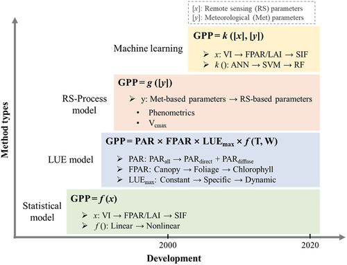
All existing RS-based GPP estimation methods can be categorized into four categories (Figure 3): statistical models, LUE models, process models integrated with RS parameters and machine learning approaches. Despite Xiao et al. (2019) regards the SIF-based model as a distinct category, these SIF-based models can be considered as input of the four categories mentioned earlier, particularly from the perspective of applying key parameters.

Figure 3. The development of remotely sensed GPP estimation. f() is linear or nonlinear equation, g() and k() are conceptual functions that represent different groups of models. The arrows (e.g. ANN→SVM→RF) only show the chronological order of application, without further meaning in model performance.

4.1. Statistical models based on RS index

The statistical model represents the earliest and most straightforward approach for GPP estimation, primarily relying on the correlation between the RS indices and GPP. Historically, the statistical model utilized the aboveground biomass or net primary productivity (NPP) in constructing the relationships with RS indices (Box, Holben, and Kalb 1989; Goward, Tucker, and Dye 1985; Paruelo et al. 1997, 2000). The statistical model underwent rapid developed with the establishment and expansion of flux observation network. Typically, a single index is employed in a statistical model, encompassing various VIs (Huang, Xiao, and Ma 2019; Huete et al. 2008; Rahman et al. 2005; Shi et al. 2017; Thanyapraneedkul et al. 2012), chlorophyll index (e.g. MTCI) (Boyd et al. 2012; Harris and Dash 2010), LAI (Hashimoto et al. 2012; Street et al. 2007), and FPAR (Hashimoto et al. 2012; Jung et al. 2008). For example, annual GPP = 615 × annual mean LAI − 376 (Hashimoto et al. 2012); GPP = a + ln(CGS-FPAR) + b, where CGS-FPAR is cumulative growing season FAPAR (Jung et al. 2008).

As mentioned above, SIF exhibits a strong representation of GPP across diverse spatiotemporal scales, purportedly surpassing traditional VIs (Li et al. 2018; Sun et al. 2017). It is utilized for GPP estimation through a statistical model based on a linear relationship (Cheng et al. 2013; Guanter et al. 2014; Liu, Guan, and Liu 2017; Rossini et al. 2010; Z. Zhang, Zhang, Porcar-Castell, et al. 2020). For instance, Guanter et al. (2014) documented a robust linear relationship (GPP = -0.10 + 3.72 × SIF) between in situ GPP observations and SIF using flux towers in America and western Europe. However, certain studies identified a nonlinear relationship between SIF and GPP (Damm et al. 2015; Li, Xiao, and He 2018), illustrating that the nonlinear SIF model in their study area exhibited superior estimation accuracy compared to the linear model (Li, Xiao, and He 2018). Biome characteristics and environmental stresses serve as the primary drivers of spatially-heterogeneous SIF-GPP relationships (Song, Wang, and Wang 2021).

The accuracy of GPP estimation in a statistical model is influenced not only by the intrinsic characteristics of the index (e.g. the saturation effect of NDVI in dense vegetation) but also by the growth patterns of plants (e.g. phenology) and environment conditions in a given geographic area (e.g. soil background). Statistical models face limitations in capturing the complexities of photosynthesis due to their reliance on a single index (or a small number of indices). Therefore, despite exhibiting relatively high regional precision, they may fall short in meeting certain requirements across large regions. Hence, some studies have incorporated additional factors into their statistical models to enhance the accuracy of GPP estimation, including radiation, temperature, and moisture (Boyd et al. 2012; Gitelson et al. 2006; Huang, Xiao, and Ma 2019; Peng, Gitelson, and Sakamoto 2013; Sims et al. 2008; Wu, Chen, and Huang 2011).

4.2. LUE model

The LUE model is a highly utilized parametric model for estimating terrestrial GPP at both regional and global scales. This model simplifies the actual photosynthesis process, wherein the absorbed PAR is partially converted to organic matter, and this conversion rate is defined as LUE (Monteith 1972). The LUE model formulates GPP as the product of PAR, FPAR, maximum LUE (LUE_max), and environmental stress (e.g. temperature and moisture, f (T, W)):

GPP = PAR × FPAR × LUE_max × f (T, W) (1)

Briefly, the LUE model consists of two parts: (1) FPAR and LUE_max, which represent the vegetation biochemical characteristics, and (2) PAR and diverse environmental stress parameters. The optimization of PAR, FPAR and LUE_max constitutes the predominant pathway in the development of the LUE model (Figure 4). Over decades, numerous models have been developed within the framework of the LUE model, including CASA (Potter et al. 1993), MODIS GPP (S. Running and Zhao 2015; S. W. Running et al. 1994), GLO-PEM (Prince and Goward 1995), TURC (Ruimy, Dedieu, and Saugier 1996), C-Fix (Veroustraete, Sabbe, and Eerens 2002), VPM (Xiao, Hollinger, et al. 2004; Xiao, Zhang, Braswell, et al. 2004), EC-LUE (Yuan et al. 2007), VPRM (Mahadevan et al. 2008), CFlux (King, Turner, and Ritts 2011), TL-LUE (He et al. 2013), CI-LUE (Wang et al. 2015), CI-EF (Almeida et al. 2018), and TS-LUE (Huang et al. 2022).

Figure 4. The development of each core parameter in the LUE model.

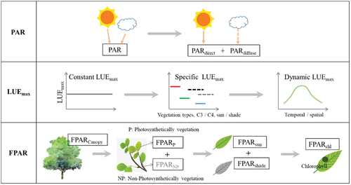
The physical meanings of FPAR used in the LUE model span from the canopy level to the chlorophyll level (see Section 3.3.1). Many existing LUE models incorporate the concept of canopy FPAR, computed using NDVI or the FPAR product of MODIS (calculated by LAI), as seen in models like CASA, MODIS-LUE, C-Fix, CFlux and EC-LUE. Xiao et al. (2004) employed FPAR_PAV in the VPM and VPRM models, while TL-LUE model used FPAR_sun and FPAR_shade (He et al. 2013). However, researchers have noticed that the PAR absorbed by green leaves (FPAR_PAV) is not entirely utilized in photosynthesis, whereas the PAR absorbed by chlorophyll (FPAR_chl) represents the total energy supplied for photosynthesis (Zhang et al. 2005). Compared to MODIS FPAR, FPAR_chl significantly enhances the accuracy of GPP estimation (Zhang et al. 2014). Similarly, Liu et al. (2017b) used EVI and NDVI to characterize FPAR_chl with a linear transformation method and discovered its superior performance in estimating GPP compared to FPAR_canopy. Each FPAR product exhibits diverse ability in representing vegetation photosynthesis (Z. Zhang, Zhang, Zhang, et al. 2020).

LUE_max is the idealized conversion rate for transforming absorbed light energy into organic matter under optimal conditions. However, the actual LUE is lower than LUE_max due to the environmental stress from factors like temperature or moisture. Consequently, the actual LUE is often characterized as the interplay of LUE_max and environmental parameters. Existing definition of LUE_max can be categorized into three types: (1) fixed value, exemplified by C-Fix and EC-LUE models; (2) fixed value adjusted for different land covers, such as MODIS-LUE and VPRM; and (3) dynamic value, such as the CFlux and CI-LUE models, which adapt LUE_max based on cloudiness, the TS-LUE model calculates LUE_max for different growing stages by using LAI (Huang et al. 2022), and some models dynamically adjust LUE_max based on EVI and albedo (H. Wang et al. 2010). Considering the nonlinear response of vegetation photosynthesis to solar radiation, Xie et al. (2023) proposed a PAR-regulated dynamic LUE_max.

LUE_max transitions gradually from a constant to dynamic value from the developmental perspective. The constant LUE_max was a significant source of uncertainty in early terrestrial GPP estimation models (Turner et al. 2005; Wang et al. 2010) due to its failure to account for spatial difference in vegetation LUE (Turner et al. 2002). Models that consider such spatial differences notably enhance GPP estimation accuracy (Madani et al. 2014; Wang et al. 2010). Dynamic LUE_max not only enhances accuracy but also aligns more closely with the real physiological laws of vegetation. Additionally, RS is increasingly utilized for LUE_max estimation. Wang et al. (2010) utilized the statistical relationship between flux observations and the maximum EVI and minimum albedo to derive spatially heterogeneous LUE_max. Huang et al. (2022a) designed an LAI-based LUE_max that varies with growth stages.

Most LUE models incorporate temperature and moisture as environmental stress factors. Temperature stress factors in LUE models encompass daily minimum temperature (T_min), daily maximum temperature (T_max), daily average temperature (T_mean) and optimum temperature for photosynthesis (T_opt). The temperature stress parameter results from transforming these factors using linear or nonlinear methods, with values ranges from 0 to 1. Each LUE model employs a unique approach to calculate and apply temperature stress parameters, and the utilization of temperature indices derived from RS is limited in LUE models. Moisture-related parameters in LUE model encompass atmosphere moisture (e.g. VPD, RH), soil moisture (e.g. SWC, SM) and vegetation moisture (e.g. LSWI, ET and PM). Moisture stress parameters such as LSWI and ET, calculable using RS, a are often favored in LUE models (Yuan et al. 2007; Zheng et al. 2018). In addition, the VPM and CFlux models consider phenology and tree age, respectively. C-Fix and adjusted EC-LUE model (Zheng et al. 2020) even account for the content of CO₂. Notably, the content of CO₂, a crucial driver of photosynthesis, is often overlooked in most LUE models (Bao et al. 2022).

In summary, due to advancements in RS and the establishment of flux tower observation networks, the LUE model has experienced rapid development (Pei et al. 2022). Concurrently, RS contributes significantly to the input parameters of the LUE model (Hilker et al. 2008). However, considerable uncertainties persist in GPP estimation using the LUE model (Yuan et al. 2014), primarily attributed to the precision of input variables, the scale effect, and the quality of validation data (Pei et al. 2022).

4.3. Process model combined with remote sensing parameters

The process model, often termed the “physical model,” simulates the exchange of carbon, water and energy in terrestrial ecosystem by integrating meteorological, vegetation structure, physiological status and soil data. Specifically, it delineates the processes of photosynthesis, respiration, evapotranspiration, and microbial decomposition, relying on assumptions and prior knowledge of vegetation, including aspects of plant developmental physiology in diverse ecosystems. Numerous process models exist, with the photosynthetic module standing as the focal point for terrestrial GPP estimation. Predominantly, process models draw upon the Farquhar photosynthesis model (Farquhar, von Caemmerer, and Berry 1980). This model utilizes the assimilation rate of CO₂ to characterize the photosynthetic rate of vegetation and incorporates parameters such as V_cmax and J_max. Initially, models relied heavily on meteorological data as input variables, but the advancement of RS introduced a novel option for process models. Mainstream process models, including SIB2 (Sellers, Randall, et al. 1996; Sellers, Tucker, et al. 1996), BEPS (Liu et al. 1997), SCOPE (van der Tol et al. 2009), and BESS (Ryu et al. 2011), incorporate RS and notably focus on developing modules for phenology and photosynthesis.

For phenological module optimization, SIB2 incorporated adjusted NDVI data to capture phenology information, building upon the foundation of SIB1 (Sellers et al. 1986). Subsequent advancements led to the development of SIB2.5 (Baker et al. 2003) and SIB3 (Baker et al. 2008). Similarly, You et al. (2019) constructed a model that substituted the meteorology-based phenological module in Biome-BGC (Running and Gower 1991; Running and Hunt 1993) with RS data.

For photosynthetic module optimization, BEPS model transferred the Farquhar photosynthesis module, a part of the FOREST-BGC model (Running and Coughlan 1988), to the canopy scale, separately simulating photosynthesis for sun leaves and shade leaves. Specifically, GPP in the BEPS model is expressed by a function incorporating variables such as LAI, canopy conductance, and mesophyll conductance (associated with V_cmax) as inputs. The BESS model integrates processes including atmosphere and canopy radiative transfer, photosynthesis, and evapotranspiration. It utilizes multisource satellite data to characterize atmosphere and ground conditions, enabling the quantification of global GPP and evapotranspiration. The BESS model employs a double-leaf canopy radiative transfer model to differentiate FPAR between sun leaves and shade leaves. It calculates photosynthesis yields in sun and shade leaves based on the photosynthesis model of C3 (Collatz et al. 1991; Farquhar, von Caemmerer, and Berry 1980) and C4 (Collatz, Ribas-Carbo, and Berry 1992). Furthermore, the BESS model optimizes key parameters V_cmax and J_max, making them seasonally dynamic values correlated with LAI (Ryu et al. 2011). In the updated BESSv2.0, a newly developed ecosystem respiration module and an optimality-based V_cmax model were integrated (Li et al. 2023). In the V_cmax module, BESSv2.0 adoptes a coordination theory and a least-cost hypothesis to estimate V_cmax, departing from the plant functional type-dependent look-up table approach (Jiang et al. 2020).

SIF also emerges as a viable option for optimizing V_cmax. Several studies have adjusted V_cmax in SCOPE by incorporating observed SIF (Verma et al. 2017; Wagle et al. 2016; Wang and Xiao 2021; Zhang et al. 2014). Moreover, other process models have assimilated SIF to enhance the accuracy of photosynthesis simulation (Bacour et al. 2019; Lee et al. 2015; Parazoo et al. 2014; Qiu et al. 2018).

4.4. Machine learning approaches

In recent times, propelled by advancements in RS, machine learning (ML) algorithms, and the proliferation of flux observation networks, an increasing number of studies have embraced ML for GPP estimation. This is particularly notable in the context of extrapolating in situ flux observations to regional and global scales. ML approaches have demonstrated their efficacy in mitigating the uncertainties associated with GPP estimation (Tramontana et al. 2015; Yu, Zhang, and Sun 2021). Their accuracy is generally equal to or better than that of traditional models (Ichii et al. 2017; Zhang et al. 2007). In addition, ML approaches, even when exclusively driven by RS data, exhibit comparably high estimation accuracy (Tramontana et al. 2016). Various algorithms have been employed for GPP estimation, including artificial neural networks (ANN) (Papale and Valentini 2003), support vector machines (SVM) (Yang et al. 2007), support vector regression (SVR) (Ueyama et al. 2013), piecewise regression models (PRM) (Wylie et al. 2007; Xiao et al. 2008; Zhang et al. 2007), model tree ensembles (MTE) (Jung et al. 2011; Liang et al. 2017), and random forest (RF) (Bodesheim et al. 2018; Wei et al. 2017). Based on RS data and ML approaches, researchers have developed models such as FLUXCOM (Jung et al. 2020; Tramontana et al. 2016) and ETES (Zhu, Zhao, and Xie 2023).

In ML approaches driven by RS inputs, NDVI/EVI, FPAR, LAI, and land cover (or vegetation types) emerge as the most widely employed variables, while SIF, phenology, NDWI, and LST find application in select models (Table 1). Notably, ML algorithms have been extended to calculate key parameters within the LUE model (Wei et al. 2017) and process model (Wolanin et al. 2019; Yuan et al. 2022). The efficacy of machine learning approaches in estimating GPP is intricately linked to the quantity and quality of reference data. Despite their proficiency in achieving high estimation accuracy, ML methods offer limited insights into the physiological mechanism of photosynthesis. Moreover, the selection of RS parameters for ML approaches remains contingent upon prior knowledge and the statistical relationships established between factors and GPP.

Table 1. The remote sensing data used in machine learning approaches for GPP estimation.

Methods	RS data	References
ANN	NOAA-AVHRR NDVI, landcover	Papale and Valentini (2003)
SVM	MODIS LST, EVI/FPAR, SWR and landcover	Yang et al. (2007)
SVR	MODIS NDVI, EVI, GR, LAI, and daytime LST	Ueyama et al. (2013)
PRM	SPOT VEGETATION NDVI and NDVI-based phenometrics	Wylie et al. (2007) and Zhang et al. (2007)
	MOD09A1, MODIS LST, EVI and LAI/FPAR	Xiao et al. (2008)
MTE	AVHRR, SeaWiFS and MERIS FPAR and FPAR-based indictors	Jung et al. (2011)
	FPAR (Z. Zhu et al. 2013) based indictors	Liang et al. (2017)
RF	SeaWiFS-FPAR, MODIS EVI and landcover	Wei et al. (2017)
	MODIS NDVI, EVI, NDWI (B.-C. Gao 1996), FPAR and LST	Bodesheim et al. (2018)
	GOSIF, NIRV (MCD43C4) and landcover	Bai et al. (2021)

Non-remotely sensed parameters are not listed. ANN: artificial neural networks; SVM: support vector machines; SVR: support vector regression; PRM: piecewise regression models; MTE: model tree ensembles; RF: random forest

5. Challenges and prospects of remotely sensed GPP estimation

5.1. Challenges

Understanding vegetation photosynthesis has advanced significantly in recent decades. Many RS-based GPP estimation methods have been created, and the corresponding products cover regional or global areas (Zhang and Ye 2021). Despite these strides, GPP estimation still grapples with substantial uncertainties (Anav et al. 2015; Schaefer et al. 2012; Zhang and Ye 2021). These uncertainties stem from various sources, with a primary focus on four key aspects: the quality of ground observations, spatiotemporal mismatch, accuracy of key parameters, and the reliability of models.

5.1.1. Quality of ground observations

Ground observations serve as the foundation for constructing models, optimizing parameters and validating the accuracy of GPP estimation. Measuring GPP directly at the ecosystem scale involves indirect assessments the net exchange between the atmosphere and terrestrial ecosystem, facilitated by over 600 eddy-covariance flux towers globally. The openly accessible FLUXNET 2015 dataset comprises 212 sites (https://fluxnet.fluxdata.org/data/fluxnet2015-dataset/), processed with stringent quality control and standardized preprocessing (Pastorello et al. 2020). However, this processing methodology introduces an error ranging from 10% to 30% (Reichstein et al. 2005; Schaefer et al. 2012). Recent studies emphasize the strong influence of non-thermal factors on nighttime vegetation respiration (Bruhn et al. 2022). This error, especially in temperature-based respiration estimation methods, may propagate into GPP estimation, particularly given the challenge of accurately measuring daytime respiration. The existing flux observation sites are still insufficient in terms of representing various vegetation types and achieving distribution uniformity. Furthermore, variations in the quantity, quality, and reference indicators (e.g. FLUXNET 2015 includes multiple reference GPPs, such as GPP_VUT_NT_MEAN and GPP_VUT _DT_MEAN) among specific sites used in different studies contribute to reduced comparability among various estimation models.

5.1.2. Spatiotemporal mismatch

The uncertainty of GPP estimation due to spatiotemporal mismatch can be delineated into three key issues. Firstly, varying spatiotemporal scales of input variables, especially in models incorporating numerous parameters, pose a challenge. For example, a significant spatial scale disparity exists between RS data and meteorological data in the LUE model. Secondly, a mismatch arises between training and final simulation, exemplified by studies translating laboratory leaf-scale results (e.g. the relationship between RS indices and GPP) to canopy and landscape scales. Generally, the leaf-scale spectral relationships are not directly applicable at larger scales due to influence from canopy structure and spatial variations (Z. Zhang, Zhang, Porcar-Castell, et al. 2020; Zhang et al. 2016). The straightforward application of small-scale parameters to a larger scale introduces errors in GPP estimation. Thirdly, a mismatch occurs between simulation results and reference data. The footprint of a flux tower spatially may not perfectly align with one or several pixels of satellite data. The flux tower’s footprint is influenced by tower height, wind speed, wind direction, surface roughness and atmospheric stability (Schmid 2002). The typical footprint of a flux tower longitudinally extends from 100 to 2000 m, while the spatial resolution of RS often ranges from 250 to 8000 m (Baldocchi et al. 2001). In numerous scenarios, the flux tower’s footprint does not align well with RS pixels, especially in areas with complex topography and land cover.

5.1.3. Quality of remotely sensed parameters

As crucial inputs of GPP estimation models, the quality and spatiotemporal resolution of remotely sensed parameters introduce significant uncertainties in GPP calculations (Zhao, Running, and Nemani 2006). The precision of widely used parameters such as VI, LAI, FPAR, LUE and SIF remains limited. For example, the precision of satellite LAI products is limited, RS-derived LAI products exhibit constrained precision, with median accuracy indicators approximately R² = 0.62 across all biome types (Fang et al. 2019). Despite evolving with an enhanced understanding of photosynthesis, bringing these parameters closer to the real photosynthesis process, their detailed accuracy requires further improvement. For instance, FPAR is divided into FPAR_canopy, FPAR_leaf and FPAR_chl, LUE is divided into LUE_sun and LUE_shade, and PAR is divided into direct PAR (PAR_direct) and diffuse PAR (PAR_diffuse) (Figure 4). While existing parameters were designed to characterize the light transmission stage (e.g. FPAR, SIF and PRI as indicators of radiation absorption and transmission), parameters delineating the biochemical process, such as V_cmax and J_max, are currently lacking. Consequently, further research on remotely sensed indices that effectively represent the real GPP is imperative.

5.1.4. The ability to represent photosynthesis

Existing GPP estimation models simplify the intricate photosynthetic process to some degree based on different assumptions. Spatial differences in terrestrial ecosystems and the complexity of photosynthesis undermine the efficacy of these assumptions, resulting in substantial errors in GPP estimation. For instance, the early LUE model assumed a constant theoretical LUE_max. However, recent studies increasingly view LUE_max as a spatiotemporally dynamic value, and different assumptions introduce varied environmental stress factors in the LUE model (Pei et al. 2022). SIF-based models also face numerous challenges due to the unstable relationship between SIF and GPP, influenced by the spatiotemporal scale, environmental stress, and vegetation type (Xiao et al. 2019). Meanwhile, intricate interplay existed among photosynthesis, thermal dissipation, and SIF (Maxwell and Johnson 2000), which contributes to the unclear mechanistic connection between GPP and SIF (Porcar-Castell et al. 2014).A comparable situation is observed between LUE and PRI.

5.2. Prospects

5.2.1. Comprehensive observations

Comprehensive observation primarily involves the collaborative observation of ground multisensors and the “Space-Air-Ground” multiscale integrated observation (Figure 5). Researchers have designed the Spectral Network (Specnet) system (Gamon 2015; Gamon et al. 2006; Zhang et al. 2021), effectively combining optical RS and flux observations to provide high-quality collaborative observations of the surface spectrum and carbon fluxes. This collaborative observation facilitates a deeper understanding of the relationship between GPP and spectral characteristics, offering an opportunity to construct a new RS index that better describes the photosynthetic process. Meanwhile, this integrated observation approach mitigates the spatiotemporal mismatch discussed earlier. The “Space-Air-Ground” integrated observation system proves to be an effective solution for addressing the scale effect between satellite and ground observations.

Figure 5. Schematic of the comprehensive observation system.

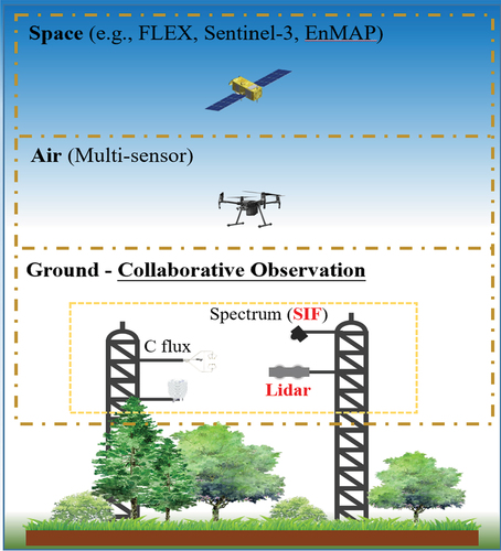
Ground observations constitute a pivotal component of this integrated observation system. Further research is imperative in three key areas: (1) optimization of processing algorithms, construction of a standardized dataset based on the existing Specnet data, and establishment of a normalized high-quality dataset of reference GPP (providing standardized training and testing datasets). (2) Facilitation of academic cooperation and the sharing of integrated observation data, coupled with an expansion of ground site distribution, especially in regions with typical vegetation. (3) Diversification of ground observation sensors. This includes the addition of SIF, COS (Carbonyl Sulfide) and Lidar sensors to enhance the Specnet framework. COS measurements are particularly valuable for quantifying terrestrial photosynthesis and estimating GPP (Kooijmans et al. 2019; Maseyk et al. 2014; Stimler et al. 2010). More importantly, COS uptake in leaves is not associated with any respiration-like emission (Stimler et al. 2010), rendering it an ideal tracer for photosynthesis. Therefore, collaborative observations of SIF, CO₂ and COS fluxes can contribute to the development of a new generation of vegetation GPP estimation models.

5.2.2. Advanced earth observation satellites

Recent advancements in multisource Earth observation satellites, including multispectral and hyperspectral satellites, lidar, and SAR, hold the potential to significantly enhance existing GPP estimation methods (Ustin and Middleton 2021). New observation missions have introduced satellites with improved capabilities, such as the PlanetScope system, providing daily global imagery at a 3 to 5 m spatial resolution, even covering “red edge” wavelengths (Roy et al. 2021). FLEX, a new-generation satellite with SIF observation capability, boasts a 100 m spatial resolution, complementing the observation of Sentinel-3 (Drusch et al. 2017). EnMAP, with 30 m spatial resolution, delivers hyperspectral data with fine spectral resolution for capturing key biochemical signals (Guanter et al. 2015). These new-generation satellites, featuring enhanced temporal, spatial, and spectral resolutions, are poised to improve GPP estimation capabilities. High temporal resolution enables the studying of the diurnal cycle of ecosystem photosynthesis and its response to various environmental stresses (Li et al. 2023). High spatial resolution provides detailed spatial information, improving GPP simulation accuracy at high resolution (Huang et al. 2022). Hyperspectral data allows the integration of xanthophyll cycle-related spectral changes, SIF, and other leaf trait-related information, such as chlorophyll and nitrogen content, to enhance GPP estimation (Dechant, Ryu, and Kang 2019). Collaborative observation and data assimilation from these new satellites offer a unique opportunity for optimizing and estimating key photosynthetic parameters, fostering a deeper understanding of photosynthesis. Meanwhile, these advanced observations are expected to further improve the performance of existing GPP estimation models (e.g. accuracy and resolution), while supporting the development of new RS indices representing GPP.

5.2.3. Big data and artificial intelligence

With the rapid development of earth observation technology (especially RS), there has been a profound expansion in data types and an explosive growth in data volume, propelling RS information technology into the era of big data (Chi et al. 2016; Ma et al. 2015; Zhang et al. 2019). In recent decades, artificial intelligence (AI) methods have become pervasive in earth sciences. As discussed in Section 4.4, traditional ML-based methods (including ANN, SVM and RF) have found widespread applications in RS-based GPP estimation. However, the limited sample data size and the number of modeled parameters constrain the generalization ability of ML, hindering its universal applicability (Zhang et al. 2019). In the realm of AI, deep learning (DL), a subset of ML employing multilayered neural networks trained on vast amounts of data, has achieved breakthroughs across various areas (LeCun, Bengio, and Hinton 2015). Convolutional neural network (CNN), recurrent neural network (RNN) and long-short term memory network (LSTM) are prominent DL models successfully implemented in RS-based vegetation monitoring and forecasting (Ferchichi et al. 2022; Lee et al. 2020; Lu et al. 2023). For example, Lee et al. (2020) compared the performance of multiple AI models in forest GPP prediction, revealing that the deep neural network (DNN) model surpassed other models like ANN, SVM, and RF. Future efforts should be directed toward synergizing the advantages of RS big data and AI to achieve automatic and real-time GPP estimation.

5.2.4. Model development

Advanced and high-quality input parameters in the future, encompassing both enhanced existing indices and newly designed indices, will play a pivotal role in elevating the performance of GPP estimation models as integrated observation systems continue to evolve. While integrating multisource products proves effective in enhancing GPP product accuracy, a more focused effort should be directed toward the development of GPP estimation models that effectively characterize the photosynthetic process, thereby advancing our understanding of terrestrial ecosystems. Consequently, future optimization endeavors should prioritize LUE, process, and SIF-based models, given their closer alignment with the real photosynthetic process. Notably, the recent P-model (Stocker et al. 2020), with a framework akin to the LUE model (Qiao et al. 2020), introduces a novel concept by adjusting GPP models through the incorporation of new high-quality parameters closely linked to photosynthesis, such as V_cmax and J_max. Despite its reliance on reanalysis data leading to a coarse resolution and moderate accuracy (Zhang et al. 2022), the P-model sparks innovative thinking for GPP estimation model enhancement. The “Space-Air-Ground” integrated observation system, coupled with improved sensors capabilities in capturing SIF, provides an opportunity to deepen our understanding of the physiological connections between SIF and GPP, paving the way for enhanced global SIF-based GPP estimation. Finally, by leveraging the complementary strengths of RS big data, AI, and physical process models, a hybrid modeling approach can be devised to yield more precise, less uncertain, and physically consistent GPP estimation models (Reichstein et al. 2019).

6. Conclusions

This paper provides a comprehensive review of research on remotely sensed GPP estimation, covering theoretical foundations, key parameters, and methodologies. Significant advancements have been made in all these aspects, especially in the development of key parameters. Parameters such as LAI, PAR, LUE, FPAR and other parameters have been further segmented to accommodate diverse scenarios, while the emergence of SIF, PRI and NIR_V has enhanced the precision of photosynthesis characterization. Nevertheless, several challenges persist in RS-based GPP estimation. Firstly, existing parameters often fall short in accurately characterizing the carbon reaction of vegetation photosynthesis. Additionally, the predominant emphasis in the development of most models lies in parameter optimization. However, the paramount priority should shift toward innovating the remotely sensed monitoring of the carbon reaction in vegetation photosynthesis. This innovation is pivotal for advancing key parameters and mechanistic models. Looking ahead, the integrated observation system and the evolution of RS sensors present an opportunity for advancing RS-based GPP estimation. Future research should focus on enhancing collaborative observations and establishing a “Space-Air-Ground” integrated observation system. This approach holds the potential to bolster the reliability of key remotely sensed parameters and facilitate the design of new RS indices and estimation models with an enhanced capacity to characterize vegetation photosynthesis.

Disclosure statement

No potential conflict of interest was reported by the author(s).

Data availability statement

Data will be made available on request.

Additional information

Funding

This study is funded by the National Key Research and Development Program of China (Grant No. 2020YFA0608504) and the Second Tibetan Plateau Scientific Expedition and Research Program (STEP) (Grant No. 2019QZKK0606).

Appendix A.

Symbols and acronyms used in the paper

[Cab]: Chlorophyll concentration

[N]: Nitrogen content

H⁺: Electrons generated by water splitting

J_max: Maximum electron transport rate (μmol m⁻² s⁻¹)

Ta: air temperature

T_max: daily maximum temperature

T_mean: daily average temperature

T_min: daily minimum temperature

T_opt: optimum temperature for photosynthesis

V_cmax: Maximum carboxylation rate (μmol m⁻² s⁻¹)

ADP: adenosine diphosphate

ANN: artificial neural networks

APAR: absorbed photosynthetically active radiation

APAR_chl: PAR absorbed by photosynthetic pigments

ATP: adenosine triphosphate

CI: clumping index

CO₂: carbon dioxide

CNN: convolutional neural network

DL: deep learning

DNN: deep neural network

EC: eddy covariance

EVI: enhanced vegetation index

EWT: equivalent water thickness

FLD: Fraunhofer Line Discrimination

FPAR_canopy: canopy-scale FPAR

FPAR_chl: chlorophyll-scale FPAR

FPAR_foliage: leaf-scale FPAR

FPAR_green: green leaf-scale FPAR

FVC: Fractional vegetation cover

GPP: Gross primary production

LAI: Leaf area index

LAI_e: effective LAI

LAI_shade: shaded LAI

LAI_sun: sunlit LAI

Lidar: light detection and ranging

LST: land surface temperature

LSTM: long-short term memory network

LUE: Light use efficiency

LUE_canopy: canopy-scale LUE

LUE_chl: chlorophyll-scale LUE

LUE_max: maximum light use efficiency

LUE_shade: shaded leaf LUE

LUE_sun: sunlit leaf LUE

MERIS: medium resolution imaging spectrometer

MIR: mid-infrared

MODIS: moderate resolution imaging spectroradiometer

MTCI: MERIS terrestrial chlorophyll index

MTE: model tree ensembles

NADPH: Nicotinamide adenine dinucleotide phosphate

NDVI: normalized difference vegetation index

NIR: near-infrared

NIR_V: near-infrared reflectance of terrestrial vegetation

NIR_VP: NIR_V multiplied by incoming sunlight

NPP: net primary productivity

NPQ: nonphotochemical quenching

PAR: photosynthetically active radiation

PAR_diffuse: diffuse radiation

PAR_direct: direct radiation

PAV: photosynthetically active part

PRI: photochemical reflectance index

PRM: piecewise regression models

RF: random forest

RNN: recurrent neural network

RS: remote sensing

SAR: synthetic aperture radar

SIF: Solar-induced chlorophyll fluorescence

SM: Soil moisture

SMC: soil moisture content

Specnet: spectral network

SVM: support vector machines

SVR: support vector regression

SWIR: Short-wave infrared

TIR: thermal infrared

VPD: vapor pressure deficit

Appendix B

List of reflectance-based indices calculation equations

Table

Index	Equation	References
EVI	$2.5\times \frac{{\mathrm{R}}_{\mathrm{NIR}}-{\mathrm{R}}_{\mathrm{Red}}}{{\mathrm{R}}_{\mathrm{NIR}}+6\times {\mathrm{R}}_{\mathrm{Red}}-7.5\times {\mathrm{R}}_{\mathrm{Blue}}+1}$	(Huete et al. 2002)
MTCI	$\frac{{\mathrm{R}}_{753.75}-{\mathrm{R}}_{708.75}}{{\mathrm{R}}_{708.75}+{\mathrm{R}}_{681.25}}$ where R753.75, R708.75, R681.25 are reflectance in the center wavelengths of band 8, 9 and 10 in the MERIS standard band setting	(Dash and Curran 2007)
NDVI	$\frac{{\mathrm{R}}_{\mathrm{NIR}}-{\mathrm{R}}_{\mathrm{Red}}}{{\mathrm{R}}_{\mathrm{NIR}}+{\mathrm{R}}_{\mathrm{Red}}}$	(Goward, Tucker, and Dye 1985)
NIRV	NDVI × RNIR	(Badgley, Field Christopher, and Berry Joseph 2017)
NIRVP	NIRV × PAR	(Dechant et al. 2022)
PRI	$\frac{{\mathrm{R}}_{531}-{\mathrm{R}}_{570}}{{\mathrm{R}}_{531}+{\mathrm{R}}_{570}}$	(Garbulsky et al. 2011)

References

- Ahmad, N., A. Irfan, and H. R. Ahmad. 2023. “Impact of Changing Abiotic Environment on Photosynthetic Adaptation in Plants.” In New Frontiers in Plant-Environment Interactions: Innovative Technologies and Developments, edited by T. Aftab, 385–32. Cham: Springer Nature Switzerland.
- Almeida, C. T. D., R. C. Delgado, L. S. Galvão, L. E. D. O. C. E. Aragão, and M. C. Ramos. 2018. “Improvements of the MODIS Gross Primary Productivity Model Based on a Comprehensive Uncertainty Assessment Over the Brazilian Amazonia.” ISPRS Journal of Photogrammetry and Remote Sensing 145:268–283. https://doi.org/10.1016/j.isprsjprs.2018.07.016.
- Alonso, L., L. Gomez-Chova, J. Vila-Frances, J. Amoros-Lopez, L. Guanter, J. Calpe, J. Moreno, et al. 2008. “Improved Fraunhofer Line Discrimination Method for Vegetation Fluorescence Quantification.” IEEE Geoscience and Remote Sensing Letters 5 (4): 620–624. https://doi.org/10.1109/LGRS.2008.2001180.
- Alton, P. B. 2017. “Retrieval of Seasonal Rubisco-Limited Photosynthetic Capacity at Global FLUXNET Sites from Hyperspectral Satellite Remote Sensing: Impact on Carbon Modelling.” Agricultural and Forest Meteorology 232:74–88. https://doi.org/10.1016/j.agrformet.2016.08.001.
- Alton, P. B. 2018. “Decadal Trends in Photosynthetic Capacity and Leaf Area Index Inferred from Satellite Remote Sensing for Global Vegetation Types.” Agricultural and Forest Meteorology 250-251:361–375. https://doi.org/10.1016/j.agrformet.2017.11.020.
- Anav, A., P. Friedlingstein, C. Beer, P. Ciais, A. Harper, C. Jones, G. Murray‐Tortarolo, et al. 2015. “Spatiotemporal Patterns of Terrestrial Gross Primary Production: A Review.” Reviews of Geophysics 53 (3): 785–818. https://doi.org/10.1002/2015RG000483.
- Bacour, C., F. Maignan, N. MacBean, A. Porcar‐Castell, J. Flexas, C. Frankenberg, P. Peylin, et al. 2019. “Improving Estimates of Gross Primary Productivity by Assimilating Solar-Induced Fluorescence Satellite Retrievals in a Terrestrial Biosphere Model Using a Process-Based SIF Model.” Journal of Geophysical Research: Biogeosciences 124 (11): 3281–3306. https://doi.org/10.1029/2019JG005040.
- Badgley, G., B. Field Christopher, and A. Berry Joseph. 2017. “Canopy Near-Infrared Reflectance and Terrestrial Photosynthesis.” Science Advances 3 (3): e1602244. https://doi.org/10.1126/sciadv.1602244.
- Bai, Y., S. Liang, and W. Yuan. 2021. “Estimating Global Gross Primary Production from Sun-Induced Chlorophyll Fluorescence Data and Auxiliary Information Using Machine Learning Methods, Remote Sensing.” Remote Sensing 13 (5): 963. https://doi.org/10.3390/rs13050963.
- Baker, N. R. 2008. “Chlorophyll Fluorescence: A Probe of Photosynthesis in vivo.” Annual Review of Plant Biology 59 (1): 89–113. https://doi.org/10.1146/annurev.arplant.59.032607.092759.
- Baker, I., A. S. Denning, N. Hanan, L. Prihodko, M. Uliasz, P.-L. Vidale, K. Davis, et al. 2003. “Simulated and Observed Fluxes of Sensible and Latent Heat and CO2 at the WLEF-TV Tower Using SiB2.5.” Global Change Biology 9 (9): 1262–1277. https://doi.org/10.1046/j.1365-2486.2003.00671.x.
- Baker, I. T., L. Prihodko, A. S. Denning, M. Goulden, S. Miller, and H. R. da Rocha. 2008. “Seasonal Drought Stress in the Amazon: Reconciling Models and Observations.” Journal of Geophysical Research: Biogeosciences 113 (G1): G00B01. https://doi.org/10.1029/2007JG000644.
- Baldocchi, D., E. Falge, L. Gu, R. Olson, D. Hollinger, S. Running, P. Anthoni, et al. 2001. “FLUXNET: A New Tool to Study the Temporal and Spatial Variability of Ecosystem–Scale Carbon Dioxide, Water Vapor, and Energy Flux Densities.” Bulletin of the American Meteorological Society 82 (11): 2415–2434. https://doi.org/10.1175/1520-0477(2001)082<2415:FANTTS>2.3.CO;2.
- Bao, S., T. Wutzler, S. Koirala, M. Cuntz, A. Ibrom, S. Besnard, S. Walther, et al. 2022. “Environment-Sensitivity Functions for Gross Primary Productivity in Light Use Efficiency Models.” Agricultural and Forest Meteorology 312:108708. https://doi.org/10.1016/j.agrformet.2021.108708.
- Barton, C. V. M., and P. R. J. North. 2001. “Remote Sensing of Canopy Light Use Efficiency Using the Photochemical Reflectance Index: Model and Sensitivity Analysis.” Remote Sensing of Environment 78 (3): 264–273. https://doi.org/10.1016/S0034-4257(01)00224-3.
- Beerling, D. J., and W. P. Quick. 1995. “A New Technique for Estimating Rates of Carboxylation and Electron Transport in Leaves of C3 Plants for Use in Dynamic Global Vegetation Models.” Global Change Biology 1 (4): 289–294. https://doi.org/10.1111/j.1365-2486.1995.tb00027.x.
- Beer, C., M. Reichstein, E. Tomelleri, P. Ciais, M. Jung, N. Carvalhais, C. Rödenbeck, et al. 2010. “Terrestrial Gross Carbon Dioxide Uptake: Global Distribution and Covariation with Climate.” Science 329 (5993): 834–838. https://doi.org/10.1126/science.1184984.
- Berger, K., J. Verrelst, J.-B. Féret, Z. Wang, M. Wocher, M. Strathmann, M. Danner, et al. 2020. “Crop Nitrogen Monitoring: Recent Progress and Principal Developments in the Context of Imaging Spectroscopy Missions.” Remote Sensing of Environment 242:111758. https://doi.org/10.1016/j.rse.2020.111758.
- Bodesheim, P., M. Jung, F. Gans, M. D. Mahecha, and M. Reichstein. 2018. “Upscaled Diurnal Cycles of Land–Atmosphere Fluxes: A New Global Half-Hourly Data Product.” Earth System Science Data 10 (3): 1327–1365. https://doi.org/10.5194/essd-10-1327-2018.
- Box, E. O., B. N. Holben, and V. Kalb. 1989. “Accuracy of the AVHRR Vegetation Index as a Predictor of Biomass, Primary Productivity and Net CO2 Flux.” Vegetatio 80 (2): 71–89. https://doi.org/10.1007/BF00048034.
- Boyd, D. S., S. Almond, J. Dash, P. J. Curran, R. A. Hill, and G. M. Foody. 2012. “Evaluation of Envisat Meris Terrestrial Chlorophyll Index-Based Models for the Estimation of Terrestrial Gross Primary Productivity.” IEEE Geoscience and Remote Sensing Letters 9 (3): 457–461. https://doi.org/10.1109/LGRS.2011.2170810.
- Braswell, B. H., D. S. Schimel, J. L. Privette, B. Moore, W. J. Emery, E. W. Sulzman, A. T. Hudak, et al. 1996. “Extracting Ecological and Biophysical Information from AVHRR Optical Data: An Integrated Algorithm Based on Inverse Modeling.” Journal of Geophysical Research: Atmospheres 101 (D18): 23335–23348. https://doi.org/10.1029/96JD02181.
- Bruhn, D., F. Newman, M. Hancock, P. Povlsen, M. Slot, S. Sitch, J. Drake, et al. 2022. “Nocturnal Plant Respiration is Under Strong Non-Temperature Control.” Nature Communications 13 (1): 5650. https://doi.org/10.1038/s41467-022-33370-1.
- Camps-Valls, G., M. Campos-Taberner, Á. Moreno-Martínez, S. Walther, G. Duveiller, A. Cescatti, M. D. Mahecha, et al. 2021. “A Unified Vegetation Index for Quantifying the Terrestrial Biosphere.” Science Advances 7 (9): eabc7447. https://doi.org/10.1126/sciadv.abc7447.
- Carlson, T. 2007. “An Overview of the “Triangle Method” for Estimating Surface Evapotranspiration and Soil Moisture from Satellite Imagery.” Sensors 7 (8): 1612–1629. https://doi.org/10.3390/s7081612.
- Celesti, M., C. van der Tol, S. Cogliati, C. Panigada, P. Yang, F. Pinto, U. Rascher, et al. 2018. “Exploring the Physiological Information of Sun-Induced Chlorophyll Fluorescence Through Radiative Transfer Model Inversion.” Remote Sensing of Environment 215:97–108. https://doi.org/10.1016/j.rse.2018.05.013.
- Chapin, F. S., P. A. Matson, and P. M. Vitousek. 2011. “Carbon Inputs to Ecosystems.” In Principles of Terrestrial Ecosystem Ecology, edited by F. S. Chapin, P. A. Matson, and P. M. Vitousek, 123–156. New York: Springer.
- Chapin, F. S., G. M. Woodwell, J. T. Randerson, E. B. Rastetter, G. M. Lovett, D. D. Baldocchi, D. A. Clark, et al. 2006. “Reconciling Carbon-Cycle Concepts, Terminology, and Methods.” Ecosystems (New York, NY) 9 (7): 1041–1050. https://doi.org/10.1007/s10021-005-0105-7.
- Chen, J. M. 2018. “Remote Sensing of Leaf Area Index and Clumping Index.” In Comprehensive Remote Sensing, edited by S. Liang, 53–77. Oxford: Elsevier.
- Chen, J. M., and T. A. Black. 1992. “Defining leaf area index for non-flat leaves.” Plant, Cell & Environment 15 (4): 421–429. https://doi.org/10.1111/j.1365-3040.1992.tb00992.x.
- Chen, B., J. M. Chen, and W. Ju. 2007. “Remote Sensing-Based Ecosystem–Atmosphere Simulation Scheme (EASS)—Model Formulation and Test with Multiple-Year Data.” Ecological Modelling 209 (2): 277–300. https://doi.org/10.1016/j.ecolmodel.2007.06.032.
- Cheng, J., S. Liang, and X. Meng. 2020. “Chapter 7 – Land Surface Temperature and Thermal Infrared Emissivity.” In Advanced Remote Sensing, edited by S. Liang and J. Wang, 251–295. 2nd ed. United States: Academic Press.
- Cheng, Y.-B., E. M. Middleton, Q. Zhang, K. Huemmrich, P. Campbell, L. Corp, B. Cook, et al. 2013. “Integrating Solar Induced Fluorescence and the Photochemical Reflectance Index for Estimating Gross Primary Production in a Cornfield.” Remote Sensing 5 (12): 6857–6879. https://doi.org/10.3390/rs5126857.
- Chen, J. M., C. H. Menges, and S. G. Leblanc. 2005. “Global Mapping of Foliage Clumping Index Using Multi-Angular Satellite Data.” Remote Sensing of Environment 97 (4): 447–457. https://doi.org/10.1016/j.rse.2005.05.003.
- Chen, J. M., G. Mo, J. Pisek, J. Liu, F. Deng, M. Ishizawa, D. Chan, et al. 2012. “Effects of Foliage Clumping on the Estimation of Global Terrestrial Gross Primary Productivity.” Global Biogeochemical Cycles 26 (1). https://doi.org/10.1029/2010GB003996.
- Chen, J. M., Wang, R., Liu, Y., He, L., Croft, H., Luo, X., Wang, H. et al. 2022. “Global Datasets of Leaf Photosynthetic Capacity for Ecological and Earth System Research.” Earth System Science Data Discussions 14 (9): 4077–4093. https://doi.org/10.5194/essd-14-4077-2022.
- Chi, M., A. Plaza, J. A. Benediktsson, Z. Sun, J. Shen, and Y. Zhu. 2016. “Big Data for Remote Sensing: Challenges and Opportunities.” Proceedings of the IEEE 104 (11): 2207–2219. https://doi.org/10.1109/JPROC.2016.2598228.
- Cogliati, S., W. Verhoef, S. Kraft, N. Sabater, L. Alonso, J. Vicent, J. Moreno, et al. 2015. “Retrieval of Sun-Induced Fluorescence Using Advanced Spectral Fitting Methods.” Remote Sensing of Environment 169:344–357. https://doi.org/10.1016/j.rse.2015.08.022.
- Collatz, G. J., J. T. Ball, C. Grivet, and J. A. Berry. 1991. “Physiological and Environmental Regulation of Stomatal Conductance, Photosynthesis and Transpiration: A Model That Includes a Laminar Boundary Layer.” Agricultural and Forest Meteorology 54 (2): 107–136. https://doi.org/10.1016/0168-1923(91)90002-8.
- Collatz, G. J., M. Ribas-Carbo, and J. A. Berry. 1992. “Coupled Photosynthesis-Stomatal Conductance Model for Leaves of C4 Plants.” Functional Plant Biology 19 (5): 519–538. https://doi.org/10.1071/PP9920519.
- Damm, A., J. A. N. Elbers, A. Erler, B. Gioli, K. Hamdi, R. Hutjes, M. Kosvancova, et al. 2010. “Remote Sensing of Sun-Induced Fluorescence to Improve Modeling of Diurnal Courses of Gross Primary Production (GPP).” Global Change Biology 16 (1): 171–186. https://doi.org/10.1111/j.1365-2486.2009.01908.x.
- Damm, A., L. Guanter, E. Paul-Limoges, C. van der Tol, A. Hueni, N. Buchmann, W. Eugster, et al. 2015. “Far-Red Sun-Induced Chlorophyll Fluorescence Shows Ecosystem-Specific Relationships to Gross Primary Production: An Assessment Based on Observational and Modeling Approaches.” Remote Sensing of Environment 166:91–105. https://doi.org/10.1016/j.rse.2015.06.004.
- Dash, J., and P. J. Curran. 2007. “Evaluation of the MERIS Terrestrial Chlorophyll Index (MTCI).” Advances in Space Research 39 (1): 100–104. https://doi.org/10.1016/j.asr.2006.02.034.
- Dechant, B., Y. Ryu, G. Badgley, P. Köhler, U. Rascher, M. Migliavacca, Y. Zhang, et al. 2022. “NIRVP: A Robust Structural Proxy for Sun-Induced Chlorophyll Fluorescence and Photosynthesis Across Scales.” Remote Sensing of Environment 268:112763. https://doi.org/10.1016/j.rse.2021.112763.
- Dechant, B., Y. Ryu, and M. Kang. 2019. “Making Full Use of Hyperspectral Data for Gross Primary Productivity Estimation with Multivariate Regression: Mechanistic Insights from Observations and Process-Based Simulations.” Remote Sensing of Environment 234:111435. https://doi.org/10.1016/j.rse.2019.111435.
- Dillen, S. Y., M. O. de Beeck, K. Hufkens, M. Buonanduci, and N. G. Phillips. 2012. “Seasonal Patterns of Foliar Reflectance in Relation to Photosynthetic Capacity and Color Index in Two Co-Occurring Tree Species, Quercus Rubra and Betula Papyrifera.” Agricultural and Forest Meteorology 160:60–68. https://doi.org/10.1016/j.agrformet.2012.03.001.
- Dobrowski, S. Z., J. C. Pushnik, P. J. Zarco-Tejada, and S. USTIN. 2005. “Simple Reflectance Indices Track Heat and Water Stress-Induced Changes in Steady-State Chlorophyll Fluorescence at the Canopy Scale.” Remote Sensing of Environment 97 (3): 403–414. https://doi.org/10.1016/j.rse.2005.05.006.
- Domingues, T. F., P. Meir, T. R. Feldpausch, G. Saiz, E. M. Veenendaal, F. Schrodt, M. Bird, et al. 2010. “Co-Limitation of Photosynthetic Capacity by Nitrogen and Phosphorus in West Africa Woodlands.” Plant, Cell & Environment 33 (6): 959–980. https://doi.org/10.1111/j.1365-3040.2010.02119.x.
- Dou, Y., F. Tian, J.-P. Wigneron, T. Tagesson, J. Du, M. Brandt, Y. Liu, et al. 2023. “Reliability of Using Vegetation Optical Depth for Estimating Decadal and Interannual Carbon Dynamics.” Remote Sensing of Environment 285:113390. https://doi.org/10.1016/j.rse.2022.113390.
- Drolet, G. G., K. F. Huemmrich, F. G. Hall, E. M. Middleton, T. A. Black, A. G. Barr, H. A. Margolis, et al. 2005. “A MODIS-Derived Photochemical Reflectance Index to Detect Inter-Annual Variations in the Photosynthetic Light-Use Efficiency of a Boreal Deciduous Forest.” Remote Sensing of Environment 98 (2): 212–224. https://doi.org/10.1016/j.rse.2005.07.006.
- Drolet, G. G., E. M. Middleton, K. F. Huemmrich, F. G. Hall, B. D. Amiro, A. G. Barr, T. A. Black, et al. 2008. “Regional Mapping of Gross Light-Use Efficiency Using MODIS Spectral Indices.” Remote Sensing of Environment 112 (6): 3064–3078. https://doi.org/10.1016/j.rse.2008.03.002.
- Drusch, M., J. Moreno, U. D. Bello, R. Franco, Y. Goulas, A. Huth, S. Kraft, et al. 2017. “The FLuorescence EXplorer Mission Concept—ESA’s Earth Explorer 8.” IEEE Transactions on Geoscience and Remote Sensing 55 (3): 1273–1284. https://doi.org/10.1109/TGRS.2016.2621820.
- Du, J., J. S. Kimball, R. H. Reichle, L. Jones, J. Watts, and Y. Kim. 2018. “Global Satellite Retrievals of the Near-Surface Atmospheric Vapor Pressure Deficit from AMSR-E and AMSR2.” Remote Sensing 10 (8): 1175. https://doi.org/10.3390/rs10081175.
- Du, S., L. Liu, X. Liu, X. Zhang, X. Zhang, Y. Bi, L. Zhang, et al. 2018. “Retrieval Of Global Terrestrial Solar-induced Chlorophyll Fluorescence From Tansat Satellite.” Science Bulletin 63 (22): 1502–1512. https://doi.org/10.1016/j.scib.2018.10.003.
- Evans, J. R. 1989. “Photosynthesis and Nitrogen Relationships in Leaves of C3 Plants.” Oecologia 78 (1): 9–19. https://doi.org/10.1007/BF00377192.
- Fang, H. 2021. “Canopy Clumping Index (CI): A Review of Methods, Characteristics, and Applications.” Agricultural and Forest Meteorology 303:108374. https://doi.org/10.1016/j.agrformet.2021.108374.
- Fang, H., F. Baret, S. Plummer, and G. Schaepman‐Strub. 2019. “An Overview of Global Leaf Area Index (LAI): Methods, Products, Validation, and Applications.” Reviews of Geophysics 57 (3): 739–799. https://doi.org/10.1029/2018RG000608.
- Fang, M., W. Ju, W. Zhan, T. Cheng, F. Qiu, and J. Wang. 2017. “A New Spectral Similarity Water Index for the Estimation of Leaf Water Content from Hyperspectral Data of Leaves.” Remote Sensing of Environment 196:13–27. https://doi.org/10.1016/j.rse.2017.04.029.
- Farquhar, G. D., S. von Caemmerer, and J. A. Berry. 1980. “A Biochemical Model of Photosynthetic CO2 Assimilation in Leaves of C3 Species.” Planta 149 (1): 78–90. https://doi.org/10.1007/BF00386231.
- Ferchichi, A., A. B. Abbes, V. Barra, and I. R. Farah. 2022. “Forecasting Vegetation Indices from Spatio-Temporal Remotely Sensed Data Using Deep Learning-Based Approaches: A Systematic Literature Review.” Ecological Informatics 68:101552. https://doi.org/10.1016/j.ecoinf.2022.101552.
- Filella, I., T. Amaro, J. L. Araus, and J. Peñuelas. 1996. “Relationship Between Photosynthetic Radiation-Use Efficiency of Barley Canopies and the Photochemical Reflectance Index (PRI).” Physiologia Plantarum 96 (2): 211–216. https://doi.org/10.1111/j.1399-3054.1996.tb00204.x.
- Finegan, B., M. Peña-Claros, A. de Oliveira, N. Ascarrunz, M. S. Bret‐Harte, G. Carreño‐Rocabado, F. Casanoves, et al. 2015. “Does Functional Trait Diversity Predict Above-Ground Biomass and Productivity of Tropical Forests? Testing Three Alternative Hypotheses.” Journal of Ecology 103 (1): 191–201. https://doi.org/10.1111/1365-2745.12346.
- Frankenberg, C., C. O’Dell, J. Berry, L. Guanter, J. Joiner, P. Köhler, R. Pollock, et al. 2014. “Prospects for Chlorophyll Fluorescence Remote Sensing from the Orbiting Carbon Observatory-2.” Remote Sensing of Environment 147:1–12. https://doi.org/10.1016/j.rse.2014.02.007.
- Frappart, F., J.-P. Wigneron, X. Li, X. Liu, A. Al-Yaari, L. Fan, M. Wang, et al. 2020. “Global Monitoring of the Vegetation Dynamics from the Vegetation Optical Depth (VOD): A Review, Remote Sensing.” Remote Sensing 12 (18): 2915. https://doi.org/10.3390/rs12182915.
- Fu, P., K. Meacham-Hensold, K. Guan, J. Wu, and C. Bernacchi. 2020. “Estimating Photosynthetic Traits from Reflectance Spectra: A Synthesis of Spectral Indices, Numerical Inversion, and Partial Least Square Regression.” Plant, Cell & Environment 43 (5): 1241–1258. https://doi.org/10.1111/pce.13718.
- Gamon, J. A. 2015. “Reviews and Syntheses: Optical Sampling of the Flux Tower Footprint.” Biogeosciences 12 (14): 4509–4523. https://doi.org/10.5194/bg-12-4509-2015.
- Gamon, J. A., J. Peñuelas, and C. B. Field. 1992. “A Narrow-Waveband Spectral Index That Tracks Diurnal Changes in Photosynthetic Efficiency.” Remote Sensing of Environment 41 (1): 35–44. https://doi.org/10.1016/0034-4257(92)90059-S.
- Gamon, J. A., A. F. Rahman, J. L. Dungan, M. Schildhauer, and K. Huemmrich. 2006. “Spectral Network (SpecNet)—What is It and Why Do We Need It?” Remote Sensing of Environment 103 (3): 227–235. https://doi.org/10.1016/j.rse.2006.04.003.
- Gamon, J. A., L. Serrano, and J. S. Surfus. 1997. “The Photochemical Reflectance Index: An Optical Indicator of Photosynthetic Radiation Use Efficiency Across Species, Functional Types, and Nutrient Levels.” Oecologia 112 (4): 492–501. https://doi.org/10.1007/s004420050337.
- Gao, B.-C. 1996. “NDWI—A Normalized Difference Water Index for Remote Sensing of Vegetation Liquid Water from Space.” Remote Sensing of Environment 58 (3): 257–266. https://doi.org/10.1016/S0034-4257(96)00067-3.
- Gao, L., X. Wang, B. A. Johnson, Q. Tian, Y. Wang, J. Verrelst, X. Mu, et al. 2020. “Remote Sensing Algorithms for Estimation of Fractional Vegetation Cover Using Pure Vegetation Index Values: A Review.” ISPRS Journal of Photogrammetry and Remote Sensing 159:364–377. https://doi.org/10.1016/j.isprsjprs.2019.11.018.
- Garbulsky, M. F., J. Peñuelas, J. Gamon, Y. Inoue, and I. Filella. 2011. “The Photochemical Reflectance Index (PRI) and the Remote Sensing of Leaf, Canopy and Ecosystem Radiation Use Efficiencies: A Review and Meta-Analysis.” Remote Sensing of Environment 115 (2): 281–297. https://doi.org/10.1016/j.rse.2010.08.023.
- Gitelson, A. A., Y. Peng, T. J. Arkebauer, and J. Schepers. 2014. “Relationships Between Gross Primary Production, Green LAI, and Canopy Chlorophyll Content in Maize: Implications for Remote Sensing of Primary Production.” Remote Sensing of Environment 144:65–72. https://doi.org/10.1016/j.rse.2014.01.004.
- Gitelson, A. A., A. Viña, S. B. Verma, D. C. Rundquist, T. J. Arkebauer, G. Keydan, B. Leavitt, et al. 2006. “Relationship Between Gross Primary Production and Chlorophyll Content in Crops: Implications for the Synoptic Monitoring of Vegetation Productivity.” Journal of Geophysical Research: Atmospheres 111 (D8): D08S11. https://doi.org/10.1029/2005JD006017.
- Goerner, A., M. Reichstein, and S. Rambal. 2009. “Tracking Seasonal Drought Effects on Ecosystem Light Use Efficiency with Satellite-Based PRI in a Mediterranean Forest.” Remote Sensing of Environment 113 (5): 1101–1111. https://doi.org/10.1016/j.rse.2009.02.001.
- GomezChova, L., L. AlonsoChorda, J. Amoros Lopez, Vila Frances, J., del ValleTascon, S., Calpe, J. and Moreno, J., et al. 2006. “Solar Induced Fluorescence Measurements Using A Field Spectroradiometer.” AIP Conference Proceedings 852 (1): 274–281.
- Goward, S. N., and K. F. Huemmrich. 1992. “Vegetation Canopy PAR Absorptance and the Normalized Difference Vegetation Index: An Assessment Using the SAIL Model.” Remote Sensing of Environment 39 (2): 119–140. https://doi.org/10.1016/0034-4257(92)90131-3.
- Goward, S. N., C. J. Tucker, and D. G. Dye. 1985. “North American Vegetation Patterns Observed with the NOAA-7 Advanced Very High Resolution Radiometer.” Vegetatio 64 (1): 3–14. https://doi.org/10.1007/BF00033449.
- Guanter, L., C. Frankenberg, A. Dudhia, P. E. Lewis, J. Gómez-Dans, A. Kuze, H. Suto, et al. 2012. “Retrieval and Global Assessment of Terrestrial Chlorophyll Fluorescence from GOSAT Space Measurements.” Remote Sensing of Environment 121:236–251. https://doi.org/10.1016/j.rse.2012.02.006.
- Guanter, L., H. Kaufmann, K. Segl, S. Foerster, C. Rogass, S. Chabrillat, T. Kuester, et al. 2015. “The EnMAP Spaceborne Imaging Spectroscopy Mission for Earth Observation.” Remote Sensing 7 (7): 8830–8857. https://doi.org/10.3390/rs70708830.
- Guanter, L., M. Rossini, R. Colombo, M. Meroni, C. Frankenberg, J.-E. Lee, J. Joiner, et al. 2013. “Using Field Spectroscopy to Assess the Potential of Statistical Approaches for the Retrieval of Sun-Induced Chlorophyll Fluorescence from Ground and Space.” Remote Sensing of Environment 133:52–61. https://doi.org/10.1016/j.rse.2013.01.017.
- Guanter, L., Y. Zhang, M. Jung, J. Joiner, M. Voigt, J. A. Berry, C. Frankenberg, et al. 2014. “Global and Time-Resolved Monitoring of Crop Photosynthesis with Chlorophyll Fluorescence.” Proceedings of the National Academy of Sciences 111 (14): E1327–E1333. https://doi.org/10.1073/pnas.1320008111.
- Guarini, R., C. Nichol, R. Clement, R. Loizzo, J. Grace, and M. Borghetti. 2014. “The Utility of MODIS-sPRI for Investigating the Photosynthetic Light-Use Efficiency in a Mediterranean Deciduous Forest.” International Journal of Remote Sensing 35 (16): 6157–6172. https://doi.org/10.1080/01431161.2014.950762.
- Gu, L., J. Han, J. D. Wood, C.-Y.-Y. Chang, and Y. Sun. 2019. “Sun-Induced Chl Fluorescence and Its Importance for Biophysical Modeling of Photosynthesis Based on Light Reactions.” New Phytologist 223 (3): 1179–1191. https://doi.org/10.1111/nph.15796.
- Hall, F. G., T. Hilker, and N. C. Coops. 2011. “PHOTOSYNSAT, Photosynthesis from Space: Theoretical Foundations of a Satellite Concept and Validation from Tower and Spaceborne Data.” Remote Sensing of Environment 115 (8): 1918–1925. https://doi.org/10.1016/j.rse.2011.03.014.
- Hall, F. G., K. F. Huemmrich, S. J. Goetz, P. J. Sellers, and J. E. Nickeson. 1992. “Satellite Remote Sensing of Surface Energy Balance: Success, Failures, and Unresolved Issues in FIFE.” Journal of Geophysical Research: Atmospheres 97 (D17): 19061–19089. https://doi.org/10.1029/92JD02189.
- Harris, A., and J. Dash. 2010. “The Potential of the MERIS Terrestrial Chlorophyll Index for Carbon Flux Estimation.” Remote Sensing of Environment 114 (8): 1856–1862. https://doi.org/10.1016/j.rse.2010.03.010.
- Hashimoto, H., J. L. Dungan, M. A. White, F. Yang, A. Michaelis, S. Running, R. Nemani, et al. 2008. “Satellite-Based Estimation of Surface Vapor Pressure Deficits Using MODIS Land Surface Temperature Data.” Remote Sensing of Environment 112 (1): 142–155. https://doi.org/10.1016/j.rse.2007.04.016.
- Hashimoto, H., W. Wang, C. Milesi, M. A. White, S. Ganguly, M. Gamo, R. Hirata, et al. 2012. “Exploring Simple Algorithms for Estimating Gross Primary Production in Forested Areas from Satellite Data.” Remote Sensing 4 (1): 303–326. https://doi.org/10.3390/rs4010303.
- He, L., J. M. Chen, J. Liu, T. Zheng, R. Wang, J. Joiner, S. Chou, et al. 2019. “Diverse Photosynthetic Capacity of Global Ecosystems Mapped by Satellite Chlorophyll Fluorescence Measurements.” Remote Sensing of Environment 232:111344. https://doi.org/10.1016/j.rse.2019.111344.
- He, M., W. Ju, Y. Zhou, J. Chen, H. He, S. Wang, H. Wang, et al. 2013. “Development of a Two-Leaf Light Use Efficiency Model for Improving the Calculation of Terrestrial Gross Primary Productivity.” Agricultural and Forest Meteorology 173:28–39. https://doi.org/10.1016/j.agrformet.2013.01.003.
- Hernández-Clemente, R., P. Kolari, A. Porcar-Castell, L. Korhonen, and M. Mottus. 2016. “Tracking the Seasonal Dynamics of Boreal Forest Photosynthesis Using EO-1 Hyperion Reflectance: Sensitivity to Structural and Illumination Effects.” IEEE Transactions on Geoscience and Remote Sensing 54 (9): 5105–5116. https://doi.org/10.1109/TGRS.2016.2554466.
- Hilker, T., N. C. Coops, F. G. Hall, C. J. Nichol, A. Lyapustin, T. A. Black, M. A. Wulder, et al. 2011. “Inferring Terrestrial Photosynthetic Light Use Efficiency of Temperate Ecosystems from Space.” Journal of Geophysical Research: Biogeosciences 116 (G3). https://doi.org/10.1029/2011JG001692.
- Hilker, T., N. C. Coops, M. A. Wulder, T. A. Black, and R. D. Guy. 2008. “The Use of Remote Sensing in Light Use Efficiency Based Models of Gross Primary Production: A Review of Current Status and Future Requirements.” Science of the Total Environment 404 (2–3): 411–423. https://doi.org/10.1016/j.scitotenv.2007.11.007.
- Homolová, L., Z. Malenovský, J. G. P. W. Clevers, G. García-Santos, and M. E. Schaepman. 2013. “Review of Optical-Based Remote Sensing for Plant Trait Mapping.” Ecological Complexity 15:1–16. https://doi.org/10.1016/j.ecocom.2013.06.003.
- Huang, G., Z. Li, X. Li, S. Liang, K. Yang, D. Wang, Y. Zhang, et al. 2019. “Estimating Surface Solar Irradiance From Satellites: Past, Present, And Future Perspectives.” Remote Sensing of Environment 233:111371. https://doi.org/10.1016/j.rse.2019.111371.
- Huang, L., X. Lin, S. Jiang, M. Liu, Y. Jiang, Z.-L. Li, R. Tang, et al. 2022. “A Two-Stage Light Use Efficiency Model for Improving Gross Primary Production Estimation in Agroecosystems.” Environmental Research Letters 17 (10): 104021. https://doi.org/10.1088/1748-9326/ac8b98.
- Huang, X., J. Xiao, and M. Ma. 2019. “Evaluating the Performance of Satellite-Derived Vegetation Indices for Estimating Gross Primary Productivity Using FLUXNET Observations Across the Globe.” Remote Sensing 11 (15): 1823. https://doi.org/10.3390/rs11151823.
- Huang, X., Y. Zheng, H. Zhang, S. Lin, S. Liang, X. Li, M. Ma, et al. 2022. “High Spatial Resolution Vegetation Gross Primary Production Product: Algorithm and Validation.” Science of Remote Sensing 5:100049. https://doi.org/10.1016/j.srs.2022.100049.
- Huete, A., K. Didan, T. Miura, E. P. Rodriguez, X. Gao, and L. G. Ferreira. 2002. “Overview of the Radiometric and Biophysical Performance of the MODIS Vegetation Indices.” Remote Sensing of Environment 83 (1): 195–213. https://doi.org/10.1016/S0034-4257(02)00096-2.
- Huete, A. R., N. Restrepo-Coupe, P. Ratana, K. Didan, S. R. Saleska, K. Ichii, S. Panuthai, et al. 2008. “Multiple Site Tower Flux and Remote Sensing Comparisons of Tropical Forest Dynamics in Monsoon Asia.” Agricultural and Forest Meteorology 148 (5): 748–760. https://doi.org/10.1016/j.agrformet.2008.01.012.
- Ichii, K., M. Ueyama, M. Kondo, N. Saigusa, J. Kim, M. C. Alberto, J. Ardö, et al. 2017. “New Data-driven Estimation Of Terrestrial CO2 Fluxes In Asia Using A Standardized Database Of Eddy Covariance Measurements, Remote Sensing Data, And Support Vector Regression.” Journal of Geophysical Research: Biogeosciences 122 (4): 767–795. https://doi.org/10.1002/2016JG003640.
- Jackson, T. J., and T. J. Schmugge. 1991. “Vegetation Effects on the Microwave Emission of Soils.” Remote Sensing of Environment 36 (3): 203–212. https://doi.org/10.1016/0034-4257(91)90057-D.
- Jiang, C., Y. Ryu, H. Wang, and T. F. Keenan. 2020. “An Optimality-Based Model Explains Seasonal Variation in C3 Plant Photosynthetic Capacity.” Global Change Biology 26 (11): 6493–6510. https://doi.org/10.1111/gcb.15276.
- Joiner, J., L. Guanter, R. Lindstrot, M. Voigt, A. P. Vasilkov, E. M. Middleton, K. F. Huemmrich, et al. 2013. “Global Monitoring of Terrestrial Chlorophyll Fluorescence from Moderate-Spectral-Resolution Near-Infrared Satellite Measurements: Methodology, Simulations, and Application to GOME-2.” Atmospheric Measurement Techniques 6 (10): 2803–2823. https://doi.org/10.5194/amt-6-2803-2013.
- Joiner, J., Y. Yoshida, L. Guanter, and E. M. Middleton. 2016. “New Methods for the Retrieval of Chlorophyll Red Fluorescence from Hyperspectral Satellite Instruments: Simulations And application to GOME-2 and SCIAMACHY.” Atmospheric Measurement Techniques 9 (8): 3939–3967. https://doi.org/10.5194/amt-9-3939-2016.
- Joiner, J., Y. Yoshida, A. P. Vasilkov, E. M. Middleton, P. K. E. Campbell, Y. Yoshida, A. Kuze, et al. 2012. “Filling-In of Near-Infrared Solar Lines by Terrestrial Fluorescence and Other Geophysical Effects: Simulations and Space-Based Observations from SCIAMACHY and GOSAT.” Atmospheric Measurement Techniques 5 (4): 809–829. https://doi.org/10.5194/amt-5-809-2012.
- Jones, H. G., ed. 2014. Plants and Microclimate: A Quantitative Approach to Environmental Plant Physiology. Cambridge: Cambridge University Press.
- Jung, M., M. Reichstein, H. A. Margolis, A. Cescatti, A. D. Richardson, M. A. Arain, A. Arneth, et al. 2011. “Global Patterns of Land-Atmosphere Fluxes of Carbon Dioxide, Latent Heat, and Sensible Heat Derived from Eddy Covariance, Satellite, and Meteorological Observations.” Journal of Geophysical Research: Biogeosciences 116 (G3). https://doi.org/10.1029/2010JG001566.
- Jung, M., C. Schwalm, M. Migliavacca, S. Walther, G. Camps-Valls, S. Koirala, P. Anthoni, et al. 2020. “Scaling Carbon Fluxes from Eddy Covariance Sites to Globe: Synthesis and Evaluation of the FLUXCOM Approach.” Biogeosciences 17 (5): 1343–1365. https://doi.org/10.5194/bg-17-1343-2020.
- Jung, M., M. Verstraete, N. Gobron, M. Reichstein, D. Papale, A. Bondeau, M. Robustelli, et al. 2008. “Diagnostic Assessment of European Gross Primary Production.” Global Change Biology 14 (10): 2349–2364. https://doi.org/10.1111/j.1365-2486.2008.01647.x.
- Kaiser, E., A. Morales, J. Harbinson, J. Kromdijk, E. Heuvelink, and L. F. M. Marcelis. 2015. “Dynamic Photosynthesis in Different Environmental Conditions.” Journal of Experimental Botany 66 (9): 2415–2426. https://doi.org/10.1093/jxb/eru406.
- Khan, A. M., P. C. Stoy, J. Joiner, D. Baldocchi, J. Verfaillie, M. Chen, J. A. Otkin, et al. 2022. “The Diurnal Dynamics of Gross Primary Productivity Using Observations from the Advanced Baseline Imager on the Geostationary Operational Environmental Satellite-R Series at an Oak Savanna Ecosystem.” Journal of Geophysical Research: Biogeosciences 127 (3): e2021JG006701. https://doi.org/10.1029/2021JG006701.
- Kiang, N. Y., J. Siefert, Govindjee, and R. E. Blankenship. 2007. “Spectral Signatures of Photosynthesis.” I Review of Earth Organisms Astrobiology 7 (1): 222–251. https://doi.org/10.1089/ast.2006.0105.
- King, D. A., D. P. Turner, and W. D. Ritts. 2011. “Parameterization of a Diagnostic Carbon Cycle Model for Continental Scale Application.” Remote Sensing of Environment 115 (7): 1653–1664. https://doi.org/10.1016/j.rse.2011.02.024.
- Köhler, P., C. Frankenberg, T. S. Magney, L. Guanter, J. Joiner, and J. Landgraf. 2018. “Global Retrievals of Solar-Induced Chlorophyll Fluorescence with TROPOMI: First Results and Intersensor Comparison to OCO-2.” Geophysical Research Letters 45 (19): ,10,456–10,463. https://doi.org/10.1029/2018GL079031.
- Köhler, P., L. Guanter, and J. Joiner. 2015. “A Linear Method for the Retrieval of Sun-Induced Chlorophyll Fluorescence from GOME-2 and SCIAMACHY Data.” Atmospheric Measurement Techniques 8 (6): 2589–2608. https://doi.org/10.5194/amt-8-2589-2015.
- Kooijmans, L. M. J., W. Sun, J. Aalto, K.-M. Erkkilä, K. Maseyk, U. Seibt, T. Vesala et al. 2019. “Influences of Light and Humidity on Carbonyl Sulfide-Based Estimates of Photosynthesis.” Proceedings of the National Academy of Sciences 116 (7): 2470–2475. https://doi.org/10.1073/pnas.1807600116.
- Kováč, D., A. Ač, L. Šigut, J. Peñuelas, J. Grace, and O. Urban. 2022. “Combining NDVI, PRI and the Quantum Yield of Solar-Induced Fluorescence Improves Estimations of Carbon Fluxes in Deciduous and Evergreen Forests.” Science of the Total Environment 829:154681. https://doi.org/10.1016/j.scitotenv.2022.154681.
- Lambers, H., F. S. Chapin, and T. L. Pons. 2008. “Photosynthesis.” In Plant Physiological Ecology, edited by H. Lambers, F. S. Chapin, and T. L. Pons, 11–99. New York, New York, NY: Springer.
- LeCun, Y., Y. Bengio, and G. Hinton. 2015. “Deep learning.” Nature 521 (7553): 436–444. https://doi.org/10.1038/nature14539.
- Lee, J.-E., J. A. Berry, C. van der Tol, X. Yang, L. Guanter, A. Damm, I. Baker, et al. 2015. “Simulations of Chlorophyll Fluorescence Incorporated into the C Ommunity L and M Odel Version 4.” Global Change Biology 21 (9): 3469–3477. https://doi.org/10.1111/gcb.12948.
- Lee, B., N. Kim, E.-S. Kim, K. Jang, M. Kang, J.-H. Lim, J. Cho, et al. 2020. “An Artificial Intelligence Approach to Predict Gross Primary Productivity in the Forests of South Korea Using Satellite Remote Sensing Data, Forests.” Forests 11 (9): 1000. https://doi.org/10.3390/f11091000.
- Liang, S., B. Jiang, and T. He. 2020. “Chapter 18 – Soil Moisture contents.” In Advanced Remote Sensing edited by S. Liang and J. Wang, 685–711. 2nd ed. United States: Academic Press.
- Liang, W., Y. Lü, W. Zhang, S. Li, Z. Jin, P. Ciais, B. Fu, et al. 2017. “Grassland Gross Carbon Dioxide Uptake Based on an Improved Model Tree Ensemble Approach Considering Human Interventions: Global Estimation and Covariation with Climate.” Global Change Biology 23 (7): 2720–2742. https://doi.org/10.1111/gcb.13592.
- Liang, S., and J. Wang. 2020. “Chapter 15 – Estimate of Vegetation Production of Terrestrial Ecosystem.” In Advanced Remote Sensing, edited by S. Liang and J. Wang, 581–620. 2nd ed. United States: Academic Press.
- Liang, S., D. Wang, T. He, and Y. Yu. 2019. “Remote Sensing of Earth’s Energy Budget: Synthesis and Review.” International Journal of Digital Earth 12 (7): 737–780. https://doi.org/10.1080/17538947.2019.1597189.
- Liang, S., X. Zhao, S. Liu, W. Yuan, X. Cheng, Z. Xiao, X. Zhang, et al. 2013. “A long-term Global LAnd Surface Satellite (GLASS) Data-set For Environmental Studies.” International Journal of Digital Earth 6 (sup1): 5–33. https://doi.org/10.1080/17538947.2013.805262.
- Liang, S., T. Zheng, R. Liu, H. Fang, S.-C. Tsay, and S. Running. 2006. “Estimation of Incident Photosynthetically Active Radiation from Moderate Resolution Imaging Spectrometer Data.” Journal of Geophysical Research: Atmospheres 111 (D15). https://doi.org/10.1029/2005JD006730.
- Liao, Z., B. Zhou, J. Zhu, H. Jia, and X. Fei. 2023. “A Critical Review of Methods, Principles and Progress for Estimating the Gross Primary Productivity of Terrestrial Ecosystems.” Frontiers in Environmental Science 11:11. https://doi.org/10.3389/fenvs.2023.1093095.
- Li, B., Y. Ryu, C. Jiang, B. Dechant, J. Liu, Y. Yan, X. Li, et al. 2023. “BESSv2.0: A Satellite-Based and Coupled-Process Model for Quantifying Long-Term Global Land–Atmosphere Fluxes.” Remote Sensing of Environment 295:113696. https://doi.org/10.1016/j.rse.2023.113696.
- Li, X., Y. Ryu, J. Xiao, B. Dechant, J. Liu, B. Li, S. Jeong, et al. 2023. “New-Generation Geostationary Satellite Reveals Widespread Midday Depression in Dryland Photosynthesis During 2020 Western U.S. Heatwave.” Science Advances 9 (31): eadi0775. https://doi.org/10.1126/sciadv.adi0775.
- Li, Z.-L., B.-H. Tang, H. Wu, H. Ren, G. Yan, Z. Wan, I. F. Trigo, et al. 2013. “Satellite-Derived Land Surface Temperature: Current Status and Perspectives.” Remote Sensing of Environment 131:14–37. https://doi.org/10.1016/j.rse.2012.12.008.
- Liu, J., J. M. Chen, J. Cihlar, Park, W.M. 1997. “A Process-Based Boreal Ecosystem Productivity Simulator Using Remote Sensing Inputs.” Remote Sensing of Environment 62 (2): 158–175. https://doi.org/10.1016/S0034-4257(97)00089-8.
- Liu, Y., J. M. Chen, L. He, Z. Zhang, R. Wang, C. Rogers, W. Fan, et al. 2022. “Non-Linearity Between Gross Primary Productivity and Far-Red Solar-Induced Chlorophyll Fluorescence Emitted from Canopies of Major Biomes.” Remote Sensing of Environment 271:112896. https://doi.org/10.1016/j.rse.2022.112896.
- Liu, L., L. Guan, and X. Liu. 2017. “Directly Estimating Diurnal Changes in GPP for C3 and C4 Crops Using Far-Red Sun-Induced Chlorophyll Fluorescence.” Agricultural and Forest Meteorology 232:1–9. https://doi.org/10.1016/j.agrformet.2016.06.014.
- Liu, X., and L. Liu. 2015. “Improving Chlorophyll Fluorescence Retrieval Using Reflectance Reconstruction Based on Principal Components Analysis.” IEEE Geoscience and Remote Sensing Letters 12 (8): 1645–1649. https://doi.org/10.1109/LGRS.2015.2417857.
- Liu, L., X. Liu, J. Chen, S. Du, Y. Ma, X. Qian, S. Chen, et al. 2020. “Estimating Maize GPP Using Near-Infrared Radiance of Vegetation.” Science of Remote Sensing 2:100009. https://doi.org/10.1016/j.srs.2020.100009.
- Liu, X., L. Liu, S. Zhang, and X. Zhou. 2015. “New Spectral Fitting Method for Full-Spectrum Solar-Induced Chlorophyll Fluorescence Retrieval Based on Principal Components Analysis.” Remote Sensing 7 (8): 10626–10645. https://doi.org/10.3390/rs70810626.
- Liu, Z., C. Wu, D. Peng, S. Wang, A. Gonsamo, B. Fang, W. Yuan, et al. 2017. “Improved Modeling of Gross Primary Production from a Better Representation of Photosynthetic Components in Vegetation Canopy.” Agricultural and Forest Meteorology 233:222–234. https://doi.org/10.1016/j.agrformet.2016.12.001.
- Li, X., and J. Xiao. 2019. “A Global, 0.05-Degree Product of Solar-Induced Chlorophyll Fluorescence Derived from OCO-2, MODIS, and Reanalysis Data.” Remote Sensing 11 (5): 2563. https://doi.org/10.3390/rs11212563.
- Li, X., J. Xiao, and B. He. 2018. “Chlorophyll Fluorescence Observed by OCO-2 is Strongly Related to Gross Primary Productivity Estimated from Flux Towers in Temperate Forests.” Remote Sensing of Environment 204:659–671. https://doi.org/10.1016/j.rse.2017.09.034.
- Li, X., J. Xiao, B. He, M. Altaf Arain, J. Beringer, A. R. Desai, C. Emmel, et al. 2018. “Solar-Induced Chlorophyll Fluorescence is Strongly Correlated with Terrestrial Photosynthesis for a Wide Variety of Biomes: First Global Analysis Based on OCO-2 and Flux Tower Observations.” Global Change Biology 24 (9): 3990–4008. https://doi.org/10.1111/gcb.14297.
- Long, S. P., and C. J. Bernacchi. 2003. “Gas Exchange Measurements, What Can They Tell Us About the Underlying Limitations to Photosynthesis? Procedures and Sources of Error.” Journal of Experimental Botany 54 (392): 2393–2401. https://doi.org/10.1093/jxb/erg262.
- Lu, J., G. Wang, D. Feng, and I. K. Nooni. 2023. “Improving the Gross Primary Production Estimate by Merging and Downscaling Based on Deep Learning, Forests.” Forests 14 (6): 1201. https://doi.org/10.3390/f14061201.
- Madani, N., J. S. Kimball, D. L. R. Affleck, J. Kattge, J. Graham, P. M. van Bodegom, P. B. Reich, et al. 2014. “Improving Ecosystem Productivity Modeling Through Spatially Explicit Estimation of Optimal Light Use Efficiency.” Journal of Geophysical Research: Biogeosciences 119 (9): 1755–1769. https://doi.org/10.1002/2014JG002709.
- Mahadevan, P., S. C. Wofsy, D. M. Matross, X. Xiao, A. L. Dunn, J. C. Lin, C. Gerbig, et al. 2008. “A Satellite-Based Biosphere Parameterization for Net Ecosystem CO2 Exchange: Vegetation Photosynthesis and Respiration Model (VPRM).” Global Biogeochemical Cycles 22 (2): GB2005. https://doi.org/10.1029/2006GB002735.
- Maseyk, K., J. A. Berry, D. Billesbach, J. E. Campbell, M. S. Torn, M. Zahniser, and U. Seibt. 2014. “Sources and Sinks of Carbonyl Sulfide in an Agricultural Field in the Southern Great Plains.” Proceedings of the National Academy of Sciences 111 (25): 9064–9069. https://doi.org/10.1073/pnas.1319132111.
- Ma, Y., H. Wu, L. Wang, B. Huang, R. Ranjan, A. Zomaya, W. Jie, et al. 2015. “Remote Sensing Big Data Computing: Challenges And Opportunities.” Future Generation Computer Systems 51:47–60. https://doi.org/10.1016/j.future.2014.10.029.
- Maxwell, K., and G. N. Johnson. 2000. “Chlorophyll fluorescence—a practical guide.” Journal of Experimental Botany 51 (345): 659–668. https://doi.org/10.1093/jexbot/51.345.659.
- McCree, K. J. 1971. “The Action Spectrum, Absorptance and Quantum Yield of Photosynthesis in Crop Plants.” Agricultural Meteorology 9:191–216. https://doi.org/10.1016/0002-1571(71)90022-7.
- Meroni, M., L. Busetto, R. Colombo, L. Guanter, J. Moreno, and W. Verhoef. 2010. “Performance of Spectral Fitting Methods for Vegetation Fluorescence Quantification.” Remote Sensing of Environment 114 (2): 363–374. https://doi.org/10.1016/j.rse.2009.09.010.
- Meroni, M., and R. Colombo. 2006. “Leaf Level Detection of Solar Induced Chlorophyll Fluorescence by Means of a Subnanometer Resolution Spectroradiometer.” Remote Sensing of Environment 103 (4): 438–448. https://doi.org/10.1016/j.rse.2006.03.016.
- Meroni, M., M. Rossini, L. Guanter, L. Alonso, U. Rascher, R. Colombo, J. Moreno, et al. 2009. “Remote Sensing of Solar-Induced Chlorophyll Fluorescence: Review of Methods and Applications.” Remote Sensing of Environment 113 (10): 2037–2051. https://doi.org/10.1016/j.rse.2009.05.003.
- Middleton, E. M., K. F. Huemmrich, D. R. Landis, T. A. Black, A. G. Barr, and J. H. McCaughey. 2016. “Photosynthetic Efficiency of Northern Forest Ecosystems Using a MODIS-Derived Photochemical Reflectance Index (PRI).” Remote Sensing of Environment 187:345–366. https://doi.org/10.1016/j.rse.2016.10.021.
- Mohammad Mahdi, N., and P. Babak. 2012. “Photosynthesis: How and Why?.” In Advances in Photosynthesis, edited by N. M. Mahdi, Ch. 1. Rijeka: IntechOpen.
- Mohammed, G. H., R. Colombo, E. M. Middleton, U. Rascher, C. van der Tol, L. Nedbal, Y. Goulas, et al. 2019. “Remote Sensing of Solar-Induced Chlorophyll Fluorescence (SIF) in Vegetation: 50 years of Progress.” Remote Sensing of Environment 231:111177. https://doi.org/10.1016/j.rse.2019.04.030.
- Monteith, J. L. 1972. “Solar Radiation and Productivity in Tropical Ecosystems.” The Journal of Applied Ecology 9 (3): 747–766. https://doi.org/10.2307/2401901.
- Moreno, A., F. Maselli, M. A. Gilabert, M. Chiesi, B. Martínez, and G. Seufert. 2012. “Assessment of MODIS Imagery to Track Light-Use Efficiency in a Water-Limited Mediterranean Pine Forest.” Remote Sensing of Environment 123:359–367. https://doi.org/10.1016/j.rse.2012.04.003.
- Muraoka, H., H. M. Noda, S. Nagai, T. Motohka, T. M. Saitoh, K. N. Nasahara, N. Saigusa, et al. 2013. “Spectral Vegetation Indices as the Indicator of Canopy Photosynthetic Productivity in a Deciduous Broadleaf Forest.” Journal of Plant Ecology 6 (5): 393–407. https://doi.org/10.1093/jpe/rts037.
- Nakaji, T., R. Ide, H. Oguma, N. Saigusa, and Y. Fujinuma. 2007. “Utility of Spectral Vegetation Index for Estimation of Gross CO2 Flux Under Varied Sky Conditions.” Remote Sensing of Environment 109 (3): 274–284. https://doi.org/10.1016/j.rse.2007.01.006.
- Nilson, T. 1971. “A Theoretical Analysis of the Frequency of Gaps in Plant Stands.” Agricultural Meteorology 8:25–38. https://doi.org/10.1016/0002-1571(71)90092-6.
- Papale, D., and R. Valentini. 2003. “A New Assessment of European Forests Carbon Exchanges by Eddy Fluxes and Artificial Neural Network Spatialization.” Global Change Biology 9 (4): 525–535. https://doi.org/10.1046/j.1365-2486.2003.00609.x.
- Parazoo, N. C., K. Bowman, J. B. Fisher, C. Frankenberg, D. B. A. Jones, A. Cescatti, Ó. Pérez‐Priego, et al. 2014. “Terrestrial Gross Primary Production Inferred from Satellite Fluorescence and Vegetation Models.” Global Change Biology 20 (10): 3103–3121. https://doi.org/10.1111/gcb.12652.
- Paruelo, J. M., H. E. Epstein, W. K. Lauenroth, and I. C. Burke. 1997. “ANPP Estimates from NDVI for the Central Grassland Region of the United States.” Ecology 78 (3): 953–958. https://doi.org/10.1890/0012-9658(1997)078[0953:AEFNFT]2.0.CO;2.
- Paruelo, J. M., M. Oesterheld, C. M. Di Bella, M. Arzadum, J. Lafontaine, M. Cahuepé, C. M. Rebella, et al. 2000. “Estimation of Primary Production of Subhumid Rangelands from Remote Sensing Data.” Applied Vegetation Science 3 (2): 189–195. https://doi.org/10.2307/1478997.
- Pastorello, G., C. Trotta, E. Canfora, H. Chu, D. Christianson, Y.-W. Cheah, C. Poindexter, et al. 2020. “The FLUXNET2015 Dataset and the ONEFlux Processing Pipeline for Eddy Covariance Data.” Scientific Data 7 (1): 225. https://doi.org/10.1038/s41597-020-0534-3.
- Patel, N. R. P., H. Devadas, R. Huete, A. Kumar, A. SenthilMurthy, and Y. V. N. Krishna. 2018. “Estimating Net Primary Productivity of Croplands in Indo-Gangetic Plains Using GOME-2 Sun-Induced Fluorescence and MODIS NDVI.” Current Science: A Fortnightly Journal of Research 114 (6): 5. https://doi.org/10.18520/cs/v114/i06/1333-1337.
- Pei, Y., J. Dong, Y. Zhang, W. Yuan, R. Doughty, J. Yang, D. Zhou, et al. 2022. “Evolution of Light Use Efficiency Models: Improvement, Uncertainties, and Implications.” Agricultural and Forest Meteorology 317:108905. https://doi.org/10.1016/j.agrformet.2022.108905.
- Peng, Y., A. A. Gitelson, and T. Sakamoto. 2013. “Remote Estimation of Gross Primary Productivity in Crops Using MODIS 250m Data.” Remote Sensing of Environment 128:186–196. https://doi.org/10.1016/j.rse.2012.10.005.
- Perez-Priego, O., P. J. Zarco-Tejada, J. R. Miller, G. Sepulcre-Canto, and E. Fereres. 2005. “Detection of Water Stress in Orchard Trees with a High-Resolution Spectrometer Through Chlorophyll Fluorescence In-Filling of the O/Sub 2/-A Band.” IEEE Transactions on Geoscience and Remote Sensing 43 (12): 2860–2869. https://doi.org/10.1109/TGRS.2005.857906.
- Piao, S., S. Sitch, P. Ciais, P. Friedlingstein, P. Peylin, X. Wang, A. Ahlström, et al. 2013. “Evaluation of Terrestrial Carbon Cycle Models for Their Response to Climate Variability and to CO2 Trends.” Global Change Biology 19 (7): 2117–2132. https://doi.org/10.1111/gcb.12187.
- Plascyk, J. A., and F. C. Gabriel. 1975. “The Fraunhofer Line Discriminator MKII-An Airborne Instrument for Precise and Standardized Ecological Luminescence Measurement.” IEEE Transactions on Instrumentation and Measurement 24 (4): 306–313. https://doi.org/10.1109/TIM.1975.4314448.
- Porcar-Castell, A., E. Tyystjärvi, J. Atherton, C. van der Tol, J. Flexas, E. E. Pfündel, J. Moreno, et al. 2014. “Linking Chlorophyll a Fluorescence to Photosynthesis for Remote Sensing Applications: Mechanisms and Challenges.” Journal of Experimental Botany 65 (15): 4065–4095. https://doi.org/10.1093/jxb/eru191.
- Potter, C. S., J. T. Randerson, C. B. Field, P. A. Matson, P. M. Vitousek, H. A. Mooney, S. A. Klooster, et al. 1993. “Terrestrial Ecosystem Production: A Process Model Based on Global Satellite and Surface Data.” Global Biogeochemical Cycles 7 (4): 811–841. https://doi.org/10.1029/93GB02725.
- Prince, S. D., S. J. Goetz, R. O. Dubayah, K. P. Czajkowski, and M. Thawley. 1998. “Inference of Surface and Air Temperature, Atmospheric Precipitable Water and Vapor Pressure Deficit Using Advanced Very High-Resolution Radiometer Satellite Observations: Comparison with Field Observations.” Journal of Hydrology 212-213:230–249. https://doi.org/10.1016/S0022-1694(98)00210-8.
- Prince, S. D., and S. N. Goward. 1995. “Global Primary Production: A Remote Sensing Approach.” Journal of Biogeography 22 (4/5): 815–835. https://doi.org/10.2307/2845983.
- Qiao, S., H. Wang, I. C. Prentice, and S. P. Harrison. 2020. “Extending a First-Principles Primary Production Model to Predict Wheat Yields.” Agricultural and Forest Meteorology 287:107932. https://doi.org/10.1016/j.agrformet.2020.107932.
- Qiu, B., Y. Xue, J. B. Fisher, W. Guo, J. A. Berry, and Y. Zhang. 2018. “Satellite Chlorophyll Fluorescence and Soil Moisture Observations Lead to Advances in the Predictive Understanding of Global Terrestrial Coupled Carbon-Water Cycles.” Global Biogeochemical Cycles 32 (3): 360–375. https://doi.org/10.1002/2017GB005744.
- Rahman, A. F., V. D. Cordova, J. A. Gamon, H. P. Schmid, and D. A. Sims. 2004. “Potential of MODIS Ocean Bands for Estimating CO2 Flux from Terrestrial Vegetation: A Novel Approach.” Geophysical Research Letters 31 (10). https://doi.org/10.1029/2004GL019778.
- Rahman, A. F., D. A. Sims, V. D. Cordova, and B. Z. El‐Masri. 2005. “Potential of MODIS EVI and surface temperature for directly estimating per-pixel ecosystem C fluxes.” Geophysical Research Letters 32 (19): L19404. https://doi.org/10.1029/2005GL024127.
- Reichstein, M., G. Camps-Valls, B. Stevens, M. Jung, J. Denzler, N. Carvalhais, et al. 2019. “Deep Learning and Process Understanding for Data-Driven Earth System Science.” Nature 566 (7743): 195–204. https://doi.org/10.1038/s41586-019-0912-1.
- Reichstein, M., E. Falge, D. Baldocchi, D. Papale, M. Aubinet, P. Berbigier, C. Bernhofer, et al. 2005. “On the Separation of Net Ecosystem Exchange into Assimilation and Ecosystem Respiration: Review and Improved Algorithm.” Global Change Biology 11 (9): 1424–1439. https://doi.org/10.1111/j.1365-2486.2005.001002.x.
- Ronggao, L., L. Shunlin, H. Honglin, J. Liu, and T. Zheng. 2008. “Mapping Incident Photosynthetically Active Radiation from MODIS Data Over China.” Remote Sensing of Environment 112 (3): 998–1009. https://doi.org/10.1016/j.rse.2007.07.021.
- Rossini, M., M. Meroni, M. Migliavacca, G. Manca, S. Cogliati, L. Busetto, V. Picchi, et al. 2010. “High Resolution Field Spectroscopy Measurements for Estimating Gross Ecosystem Production in a Rice Field.” Agricultural and Forest Meteorology 150 (9): 1283–1296. https://doi.org/10.1016/j.agrformet.2010.05.011.
- Rouse, J. W. 1974. “Monitoring the Vernal Advancements and Retrogradation of Natural Vegetation.” NASA-CR-139243 PR-7 E74-10676: NASA/GSFC .
- Roy, D. P., H. Huang, R. Houborg, and V. S. Martins. 2021. “A Global Analysis of the Temporal Availability of PlanetScope High Spatial Resolution Multi-Spectral Imagery.” Remote Sensing of Environment 264:112586. https://doi.org/10.1016/j.rse.2021.112586.
- Ruimy, A., G. Dedieu, and B. Saugier. 1996. “TURC: A Diagnostic Model of Continental Gross Primary Productivity and Net Primary Productivity.” Global Biogeochemical Cycles 10 (2): 269–285. https://doi.org/10.1029/96GB00349.
- Running, S. W., and J. C. Coughlan. 1988. “A General Model of Forest Ecosystem Processes for Regional Applications I. Hydrologic Balance, Canopy Gas Exchange and Primary Production Processes.” Ecological Modelling 42 (2): 125–154. https://doi.org/10.1016/0304-3800(88)90112-3.
- Running, S. W., and S. T. Gower. 1991. “FOREST-BGC, a General Model of Forest Ecosystem Processes for Regional Applications. II. Dynamic Carbon Allocation and Nitrogen Budgets.” Tree Physiology 9 (1–2): 147–160. https://doi.org/10.1093/treephys/9.1-2.147.
- Running, S. W., and E. R. Hunt Jr. 1993. “Generalization of a Forest Ecosystem Process Model for Other Biomes, BIOME-BGC, and an Application for Global-Scale Models.” In Scaling Physiological Processes: Leaf to Globe, edited by J. R. Ehleringer and C. B. Field, 141–158. San Diego: Academic Press.
- Running, S. W., C. O. Justice, V. Salomonson, D. Hall, J. Barker, Y. J. Kaufmann, A. H. Strahler, et al. 1994. “Terrestrial Remote Sensing Science and Algorithms Planned for EOS/MODIS.” International Journal of Remote Sensing 15 (17): 3587–3620. https://doi.org/10.1080/01431169408954346.
- Running, S., and M. Zhao. 2015. “User’s Guide Daily GPP and Annual NPP (MOD17A2/A3) Products NASA Earth Observing System MODIS Land Algorithm.”
- Ryu, Y., D. D. Baldocchi, H. Kobayashi, C. van Ingen, J. Li, T. A. Black, J. Beringer, et al. 2011. “Integration of MODIS Land and Atmosphere Products with a Coupled-Process Model to Estimate Gross Primary Productivity and Evapotranspiration from 1 Km to Global Scales.” Global Biogeochemical Cycles 25 (4): GB4017. https://doi.org/10.1029/2011GB004053.
- Ryu, Y., J. A. Berry, and D. D. Baldocchi. 2019. “What is Global Photosynthesis? History, Uncertainties and Opportunities.” Remote Sensing of Environment 223:95–114. https://doi.org/10.1016/j.rse.2019.01.016.
- Schaefer, K., C. R. Schwalm, C. Williams, M. A. Arain, A. Barr, J. M. Chen, K. J. Davis, et al. 2012. “A Model-Data Comparison of Gross Primary Productivity: Results from the North American Carbon Program Site Synthesis.” Journal of Geophysical Research: Biogeosciences 117 (G3). https://doi.org/10.1029/2012JG001960.
- Schimel, D., F. D. Schneider , and JPL Carbon and Ecosystem Participants. 2019. “Flux Towers in the Sky: Global Ecology from Space.” New Phytologist 224 (2): 570–584. https://doi.org/10.1111/nph.15934.
- Schmid, H. P. 2002. “Footprint Modeling for Vegetation Atmosphere Exchange Studies: A Review and Perspective.” Agricultural and Forest Meteorology 113 (1): 159–183. https://doi.org/10.1016/S0168-1923(02)00107-7.
- Scholze, M., M. Buchwitz, W. Dorigo, L. Guanter, and S. Quegan. 2017. “Reviews and Syntheses: Systematic Earth Observations for Use in Terrestrial Carbon Cycle Data Assimilation Systems.” Biogeosciences 14 (14): 3401–3429. https://doi.org/10.5194/bg-14-3401-2017.
- Sellers, P. J., R. E. Dickinson, D. A. Randall, A. K. Betts, F. G. Hall, J. A. Berry, G. J. Collatz, et al. 1997. “Modeling the Exchanges of Energy, Water, and Carbon Between Continents and the Atmosphere.” Science 275 (5299): 502–509. https://doi.org/10.1126/science.275.5299.502.
- Sellers, P. J., Y. Mintz, Y. C. Sud, and A. Dalcher. 1986. “A Simple Biosphere Model (SIB) for Use within General Circulation Models.” Journal of the Atmospheric Sciences 43 (6): 505–531. https://doi.org/10.1175/1520-0469(1986)043<0505:ASBMFU>2.0.CO;2.
- Sellers, P. J., D. A. Randall, G. J. Collatz, J. A. Berry, C. B. Field, D. A. Dazlich, C. Zhang, et al. 1996. “A Revised Land Surface Parameterization (SiB2) for Atmospheric GCMS. Part I: Model Formulation.” Journal of Climate 9 (4): 676–705. https://doi.org/10.1175/1520-0442(1996)009<0676:ARLSPF>2.0.CO;2.
- Sellers, P. J., C. J. Tucker, G. J. Collatz, S. O. Los, C. O. Justice, D. A. Dazlich, D. A. Randall, et al. 1996. “A Revised Land Surface Parameterization (SiB2) for Atmospheric GCMS. Part II: The Generation of Global Fields of Terrestrial Biophysical Parameters from Satellite Data.” Journal of Climate 9 (4): 706–737. https://doi.org/10.1175/1520-0442(1996)009<0706:ARLSPF>2.0.CO;2.
- Serbin, S. P., D. N. Dillaway, E. L. Kruger, and P. A. Townsend. 2012. “Leaf Optical Properties Reflect Variation in Photosynthetic Metabolism and Its Sensitivity to Temperature.” Journal of Experimental Botany 63 (1): 489–502. https://doi.org/10.1093/jxb/err294.
- Serbin, S. P., A. Singh, A. R. Desai, S. G. Dubois, A. D. Jablonski, C. C. Kingdon, E. L. Kruger, et al. 2015. “Remotely Estimating Photosynthetic Capacity, and Its Response to Temperature, in Vegetation Canopies Using Imaging Spectroscopy.” Remote Sensing of Environment 167:78–87. https://doi.org/10.1016/j.rse.2015.05.024.
- Shi, H., L. Li, D. Eamus, A. Huete, J. Cleverly, X. Tian, Q. Yu, et al. 2017. “Assessing the Ability of MODIS EVI to Estimate Terrestrial Ecosystem Gross Primary Production of Multiple Land Cover Types.” Ecological Indicators 72:153–164. https://doi.org/10.1016/j.ecolind.2016.08.022.
- Shoshany, M., T. Svoray, P. J. Curran, G. M. Foody, and A. Perevolotsky. 2000. “The Relationship Between ERS-2 SAR Backscatter and Soil Moisture: Generalization from a Humid to Semi-Arid Transect.” International Journal of Remote Sensing 21 (11): 2337–2343. https://doi.org/10.1080/01431160050029620.
- Siebers, M. H., N. Gomez-Casanovas, P. Fu, K. Meacham-Hensold, C. E. Moore, C. J. Bernacchi, et al. 2021. “Emerging Approaches to Measure Photosynthesis from the Leaf to the Ecosystem.” Emerging Topics in Life Sciences 5 (2): 261–274. https://doi.org/10.1042/ETLS20200292.
- Sims, D. A., and J. A. Gamon. 2003. “Estimation of Vegetation Water Content and Photosynthetic Tissue Area from Spectral Reflectance: A Comparison of Indices Based on Liquid Water and Chlorophyll Absorption Features.” Remote Sensing of Environment 84 (4): 526–537. https://doi.org/10.1016/S0034-4257(02)00151-7.
- Sims, D. A., A. F. Rahman, V. D. Cordova, B. Elmasri, D. Baldocchi, P. Bolstad, L. Flanagan, et al. 2008. “A New Model of Gross Primary Productivity for North American Ecosystems Based Solely on the Enhanced Vegetation Index and Land Surface Temperature from MODIS.” Remote Sensing of Environment 112 (4): 1633–1646. https://doi.org/10.1016/j.rse.2007.08.004.
- Song, C., M. P. Dannenberg, and T. Hwang. 2013. “Optical Remote Sensing of Terrestrial Ecosystem Primary Productivity.” Progress in Physical Geography: Earth and Environment 37 (6): 834–854. https://doi.org/10.1177/0309133313507944.
- Song, Y., L. Wang, and J. Wang. 2021. “Improved Understanding of the Spatially-Heterogeneous Relationship Between Satellite Solar-Induced Chlorophyll Fluorescence and Ecosystem Productivity.” Ecological Indicators 129:107949. https://doi.org/10.1016/j.ecolind.2021.107949.
- Srivastava, P. K. 2017. “Satellite Soil Moisture: Review of Theory and Applications in Water Resources.” Water Resources Management 31 (10): 3161–3176. https://doi.org/10.1007/s11269-017-1722-6.
- Stagakis, S., N. Markos, O. Sykioti, and A. Kyparissis. 2014. “Tracking Seasonal Changes of Leaf and Canopy Light Use Efficiency in a Phlomis Fruticosa Mediterranean Ecosystem Using Field Measurements and Multi-Angular Satellite Hyperspectral Imagery.” ISPRS Journal of Photogrammetry and Remote Sensing 97:138–151. https://doi.org/10.1016/j.isprsjprs.2014.08.012.
- Stimler, K., S. A. Montzka, J. A. Berry, Y. Rudich, and D. Yakir. 2010. “Relationships Between Carbonyl Sulfide (COS) and CO2 During Leaf Gas Exchange.” New Phytologist 186 (4): 869–878. https://doi.org/10.1111/j.1469-8137.2010.03218.x.
- Stocker, B. D., H. Wang, N. G. Smith, S. P. Harrison, T. F. Keenan, D. Sandoval, T. Davis, et al. 2020. “P-Model V1.0: An Optimality-Based Light Use Efficiency Model for Simulating Ecosystem Gross Primary Production.” Geoscientific Model Development 13 (3): 1545–1581. https://doi.org/10.5194/gmd-13-1545-2020.
- Street, L. E., G. R. Shaver, M. Williams, and M. T. Van wijk. 2007. “What is the Relationship Between Changes in Canopy Leaf Area and Changes in Photosynthetic CO2 Flux in Arctic Ecosystems?” Journal of Ecology 95 (1): 139–150. https://doi.org/10.1111/j.1365-2745.2006.01187.x.
- Sun, Y., C. Frankenberg, J. D. Wood, D. S. Schimel, M. Jung, L. Guanter, D. T. Drewry, et al. 2017. “OCO-2 Advances Photosynthesis Observation from Space via Solar-Induced Chlorophyll Fluorescence.” Science 358 (6360): eaam5747. https://doi.org/10.1126/science.aam5747.
- Sun, Z., X. Wang, X. Zhang, H. Tani, E. Guo, S. Yin, T. Zhang, et al. 2019. “Evaluating and Comparing Remote Sensing Terrestrial GPP Models for Their Response to Climate Variability and CO2 Trends.” Science of the Total Environment 668:696–713. https://doi.org/10.1016/j.scitotenv.2019.03.025.
- Tan, C., A. Samanta, X. Jin, L. Tong, C. Ma, W. Guo, Y. Knyazikhin, et al. 2013. “Using Hyperspectral Vegetation Indices to Estimate the Fraction of Photosynthetically Active Radiation Absorbed by Corn Canopies.” International Journal of Remote Sensing 34 (24): 8789–8802. https://doi.org/10.1080/01431161.2013.853143.
- Tao, X., Z. Xiao, and W. Fan. 2020. “Chapter 11 - Fraction of Absorbed Photosynthetically Active Radiation.” In Advanced Remote Sensing, edited by S. Liang and J. Wang, 447–476. 2nd ed. United States: Academic Press.
- Teubner, I. E., M. Forkel, G. Camps-Valls, M. Jung, D. G. Miralles, G. Tramontana, R. van der Schalie, et al. 2019. “A Carbon Sink-Driven Approach to Estimate Gross Primary Production from Microwave Satellite Observations.” Remote Sensing of Environment 229:100–113. https://doi.org/10.1016/j.rse.2019.04.022.
- Thanyapraneedkul, J., K. Muramatsu, M. Daigo, S. Furumi, N. Soyama, K. Nasahara, H. Muraoka, et al. 2012. “A Vegetation Index to Estimate Terrestrial Gross Primary Production Capacity for the Global Change Observation Mission-Climate (GCOM-C)/second-Generation Global Imager (SGLI) Satellite Sensor.” Remote Sensing 4 (12): 3689–3720. https://doi.org/10.3390/rs4123689.
- Thenkabail, P. S., J. G. Lyon, and A. Huete. 2011. Hyperspectral Remote Sensing of Vegetation. Boca Raton, FL: CRC Press.
- Tramontana, G., K. Ichii, G. Camps-Valls, E. Tomelleri, and D. Papale. 2015. “Uncertainty Analysis of Gross Primary Production Upscaling Using Random Forests, Remote Sensing and Eddy Covariance Data.” Remote Sensing of Environment 168:360–373. https://doi.org/10.1016/j.rse.2015.07.015.
- Tramontana, G., M. Jung, C. R. Schwalm, K. Ichii, G. Camps-Valls, B. Ráduly, M. Reichstein, et al. 2016. “Predicting Carbon Dioxide and Energy Fluxes Across Global FLUXNET Sites with Regression Algorithms.” Biogeosciences 13 (14): 4291–4313. https://doi.org/10.5194/bg-13-4291-2016.
- Turner, D. P., S. T. Gower, W. B. Cohen, M. Gregory, and T. K. Maiersperger. 2002. “Effects of Spatial Variability in Light Use Efficiency on Satellite-Based NPP Monitoring.” Remote Sensing of Environment 80 (3): 397–405. https://doi.org/10.1016/S0034-4257(01)00319-4.
- Turner, D. P., W. D. Ritts, W. B. Cohen, T. K. Maeirsperger, S. T. Gower, A. A. Kirschbaum, S. W. Running, et al. 2005. “Site-Level Evaluation of Satellite-Based Global Terrestrial Gross Primary Production and Net Primary Production Monitoring.” Global Change Biology 11 (4): 666–684. https://doi.org/10.1111/j.1365-2486.2005.00936.x.
- Ueyama, M., K. Ichii, H. Iwata, E. S. Euskirchen, D. Zona, A. V. Rocha, Y. Harazono, et al. 2013. “Upscaling Terrestrial Carbon Dioxide Fluxes in Alaska with Satellite Remote Sensing and Support Vector Regression.” Journal of Geophysical Research: Biogeosciences 118 (3): 1266–1281. https://doi.org/10.1002/jgrg.20095.
- Ulsig, L., C. J. Nichol, K. F. Huemmrich, D. Landis, E. Middleton, A. Lyapustin, I. Mammarella, et al. 2017. “Detecting Inter-Annual Variations in the Phenology of Evergreen Conifers Using Long-Term MODIS Vegetation Index Time Series.” Remote Sensing 9 (1): 49. https://doi.org/10.3390/rs9010049.
- Ustin, S. L., and E. M. Middleton. 2021. “Current and Near-Term Advances in Earth Observation for Ecological Applications.” Ecological Processes 10 (1): 1. https://doi.org/10.1186/s13717-020-00255-4.
- van der Tol, C., M. Rossini, S. Cogliati, W. Verhoef, R. Colombo, U. Rascher, G. Mohammed, et al. 2016. “A Model and Measurement Comparison of Diurnal Cycles of Sun-Induced Chlorophyll Fluorescence of Crops.” Remote Sensing of Environment 186:663–677. https://doi.org/10.1016/j.rse.2016.09.021.
- van der Tol, C., W. Verhoef, J. Timmermans, A. Verhoef, and Z. Su. 2009. “An Integrated Model of Soil-Canopy Spectral Radiances, Photosynthesis, Fluorescence, Temperature and Energy Balance.” Biogeosciences 6 (12): 3109–3129. https://doi.org/10.5194/bg-6-3109-2009.
- van der Tol, C., N. Vilfan, D. Dauwe, M. P. Cendrero-Mateo, and P. Yang. 2019. “The Scattering and Re-Absorption of Red and Near-Infrared Chlorophyll Fluorescence in the Models Fluspect and SCOPE.” Remote Sensing of Environment 232:111292. https://doi.org/10.1016/j.rse.2019.111292.
- Van Laake, P. E., and G. A. Sanchez-Azofeifa. 2004. “Simplified Atmospheric Radiative Transfer Modelling for Estimating Incident PAR Using MODIS Atmosphere Products.” Remote Sensing of Environment 91 (1): 98–113. https://doi.org/10.1016/j.rse.2004.03.002.
- Verma, M., D. Schimel, B. Evans, C. Frankenberg, J. Beringer, D. T. Drewry, T. Magney, et al. 2017. “Effect of Environmental Conditions on the Relationship Between Solar-Induced Fluorescence and Gross Primary Productivity at an OzFlux Grassland Site.” Journal of Geophysical Research: Biogeosciences 122 (3): 716–733. https://doi.org/10.1002/2016JG003580.
- Veroustraete, F., H. Sabbe, and H. Eerens. 2002. “Estimation of Carbon Mass Fluxes Over Europe Using the C-Fix Model and Euroflux Data.” Remote Sensing of Environment 83 (3): 376–399. https://doi.org/10.1016/S0034-4257(02)00043-3.
- Wagle, P., Y. Zhang, C. Jin, and X. Xiao. 2016. “Comparison of Solar-Induced Chlorophyll Fluorescence, Light-Use Efficiency, and Process-Based GPP Models in Maize.” Ecological Applications 26 (4): 1211–1222. https://doi.org/10.1890/15-1434.
- Walker, A. P., A. P. Beckerman, L. Gu, J. Kattge, L. A. Cernusak, T. F. Domingues, J. C. Scales, et al. 2014. “The Relationship of Leaf Photosynthetic Traits – Vcmax and Jmax – to Leaf Nitrogen, Leaf Phosphorus, and Specific Leaf Area: A Meta-Analysis and Modeling Study.” Ecology and Evolution 4 (16): 3218–3235. https://doi.org/10.1002/ece3.1173.
- Walker, M. D., C. H. Wahren, R. D. Hollister, G. H. R. Henry, L. E. Ahlquist, J. M. Alatalo, M. S. Bret-Harte, et al. 2006. “Plant Community Responses to Experimental Warming Across the Tundra Biome.” Proceedings of the National Academy of Sciences 103 (5): 1342–1346. https://doi.org/10.1073/pnas.0503198103.
- Wang, S., K. Huang, H. Yan, H. Yan, L. Zhou, H. Wang, J. Zhang, et al. 2015. “Improving the Light Use Efficiency Model for Simulating Terrestrial Vegetation Gross Primary Production by the Inclusion of Diffuse Radiation Across Ecosystems in China.” Ecological Complexity 23:1–13. https://doi.org/10.1016/j.ecocom.2015.04.004.
- Wang, H., G. Jia, C. Fu, J. Feng, T. Zhao, and Z. Ma. 2010. “Deriving Maximal Light Use Efficiency from Coordinated Flux Measurements and Satellite Data for Regional Gross Primary Production Modeling.” Remote Sensing of Environment 114 (10): 2248–2258. https://doi.org/10.1016/j.rse.2010.05.001.
- Wang, Y. P., and R. Leuning. 1998. “A Two-Leaf Model for Canopy Conductance, Photosynthesis and Partitioning of Available Energy I: Model Description and Comparison with a Multi-Layered Model.” Agricultural and Forest Meteorology 91 (1): 89–111. https://doi.org/10.1016/S0168-1923(98)00061-6.
- Wang, D., S. Liang, Y. Zhang, X. Gao, M. G. L. Brown, and A. Jia. 2020. “A New Set of MODIS Land Products (MCD18): Downward Shortwave Radiation and Photosynthetically Active Radiation.” Remote Sensing 12 (1): 168. https://doi.org/10.3390/rs12010168.
- Wang, Y., R. Li, J. Hu, Y. Fu, J. Duan, and Y. Cheng. 2021. “Daily Estimation of Gross Primary Production Under All Sky Using a Light Use Efficiency Model Coupled with Satellite Passive Microwave Measurements.” Remote Sensing of Environment 267:112721. https://doi.org/10.1016/j.rse.2021.112721.
- Wang, H., and J. Xiao. 2021. “Improving the Capability of the SCOPE Model for Simulating Solar-Induced Fluorescence and Gross Primary Production Using Data from OCO-2 and Flux Towers.” Remote Sensing 13 (4): 794. https://doi.org/10.3390/rs13040794.
- Wang, S., Y. Zhang, W. Ju, B. Qiu, and Z. Zhang. 2021. “Tracking the Seasonal and Inter-Annual Variations of Global Gross Primary Production During Last Four Decades Using Satellite Near-Infrared Reflectance Data.” Science of the Total Environment 755:142569. https://doi.org/10.1016/j.scitotenv.2020.142569.
- Wei, S., C. Yi, W. Fang, and G. Hendrey. 2017. “A Global Study of GPP Focusing on Light-Use Efficiency in a Random Forest Regression Model.” Ecosphere 8 (5): e01724. https://doi.org/10.1002/ecs2.1724.
- Welp, L. R., R. F. Keeling, H. A. J. Meijer, A. F. Bollenbacher, S. C. Piper, K. Yoshimura, R. J. Francey, et al. 2011. “Interannual Variability in the Oxygen Isotopes of Atmospheric CO2 Driven by El Niño.” Nature 477 (7366): 579–582. https://doi.org/10.1038/nature10421.
- Wolanin, A., G. Camps-Valls, L. Gómez-Chova, G. Mateo-García, C. van der Tol, Y. Zhang, L. Guanter, et al. 2019. “Estimating Crop Primary Productivity with Sentinel-2 and Landsat 8 Using Machine Learning Methods Trained with Radiative Transfer Simulations.” Remote Sensing of Environment 225:441–457. https://doi.org/10.1016/j.rse.2019.03.002.
- Wu, C., J. M. Chen, and N. Huang. 2011. “Predicting Gross Primary Production from the Enhanced Vegetation Index and Photosynthetically Active Radiation: Evaluation and Calibration.” Remote Sensing of Environment 115 (12): 3424–3435. https://doi.org/10.1016/j.rse.2011.08.006.
- Wu, G., K. Guan, C. Jiang, H. Kimm, G. Miao, C. J. Bernacchi, C. E. Moore, et al. 2022. “Attributing Differences of Solar-Induced Chlorophyll Fluorescence (SIF)-Gross Primary Production (GPP) Relationships Between Two C4 Crops: Corn and Miscanthus.” Agricultural and Forest Meteorology 323:109046. https://doi.org/10.1016/j.agrformet.2022.109046.
- Wylie, B. K., E. A. Fosnight, T. G. Gilmanov, A. B. Frank, J. A. Morgan, M. R. Haferkamp, T. P. Meyers, et al. 2007. “Adaptive Data-Driven Models for Estimating Carbon Fluxes in the Northern Great Plains.” Remote Sensing of Environment 106 (4): 399–413. https://doi.org/10.1016/j.rse.2006.09.017.
- Xia, J., S. Niu, P. Ciais, I. A. Janssens, J. Chen, C. Ammann, A. Arain, et al. 2015. “Joint Control of Terrestrial Gross Primary Productivity by Plant Phenology and Physiology.” Proceedings of the National Academy of Sciences of the United States of America 112 (9): 2788. https://doi.org/10.1073/pnas.1413090112.
- Xiao, J., F. Chevallier, C. Gomez, L. Guanter, J. A. Hicke, A. R. Huete, K. Ichii, et al. 2019. “Remote Sensing of the Terrestrial Carbon Cycle: A Review of Advances Over 50 Years.” Remote Sensing of Environment 233:111383. https://doi.org/10.1016/j.rse.2019.111383.
- Xiao, X., D. Hollinger, J. Aber, M. Goltz, E. A. Davidson, Q. Zhang, B. Moore, et al. 2004. “Satellite-Based Modeling of Gross Primary Production in an Evergreen Needleleaf Forest.” Remote Sensing of Environment 89 (4): 519–534. https://doi.org/10.1016/j.rse.2003.11.008.
- Xiao, X., C. Jin, and J. Dong. 2014. “Gross Primary Production of Terrestrial Vegetation.” In Biophysical Applications of Satellite Remote Sensing, edited by J. M. Hanes, 127–148. Berlin Heidelberg, Berlin, Heidelberg: Springer.
- Xiao, X., Q. Zhang, B. Braswell,Urbanski, S., Boles, S., Wofsy, S., Moore III, B. and Ojima, D. et al. 2004. “Modeling Gross Primary Production of Temperate Deciduous Broadleaf Forest Using Satellite Images and Climate Data.” Remote Sensing of Environment 91 (2): 256–270. https://doi.org/10.1016/j.rse.2004.03.010.
- Xiao, J., Q. Zhuang, D. D. Baldocchi, B. E. Law, A. D. Richardson, J. Chen, R. Oren, et al. 2008. “Estimation of Net Ecosystem Carbon Exchange for the Conterminous United States by Combining MODIS and AmeriFlux Data.” Agricultural and Forest Meteorology 148 (11): 1827–1847. https://doi.org/10.1016/j.agrformet.2008.06.015.
- Xie, X., A. Li, H. Jin, G. Yin, and X. Nan. 2018. “Derivation of Temporally Continuous Leaf Maximum Carboxylation Rate (V) from the Sunlit Leaf Gross Photosynthesis Productivity Through Combining BEPS Model with Light Response Curve at Tower Flux Sites.” Agricultural and Forest Meteorology 259:82–94. https://doi.org/10.1016/j.agrformet.2018.04.017.
- Xie, Z., C. Zhao, W. Zhu, H. Zhang, and Y. H. Fu. 2023. “A Radiation-Regulated Dynamic Maximum Light Use Efficiency for Improving Gross Primary Productivity Estimation.” Remote Sensing 15 (5): 1176. https://doi.org/10.3390/rs15051176.
- Yang, F., K. Ichii, M. A. White, H. Hashimoto, A. R. Michaelis, P. Votava, A.-X. Zhu, et al. 2007. “Developing a Continental-Scale Measure of Gross Primary Production by Combining MODIS and AmeriFlux Data Through Support Vector Machine Approach.” Remote Sensing of Environment 110 (1): 109–122. https://doi.org/10.1016/j.rse.2007.02.016.
- Yang, P., E. Prikaziuk, W. Verhoef, and C. van der Tol. 2021. “SCOPE 2.0: A Model To Simulate Vegetated Land Surface Fluxes And Satellite Signals.” Geoscientific Model Development 14 (7): 4697–4712. https://doi.org/10.5194/gmd-14-4697-2021.
- Yan, H., S. Q. Wang, D. Billesbach, W. Oechel, J. H. Zhang, T. Meyers, T. A. Martin, et al. 2012. “Global Estimation of Evapotranspiration Using a Leaf Area Index-Based Surface Energy and Water Balance Model.” Remote Sensing of Environment 124:581–595. https://doi.org/10.1016/j.rse.2012.06.004.
- Yebra, M., A. Van Dijk, R. Leuning, A. Huete, and J. P. Guerschman. 2013. “Evaluation Of Optical Remote Sensing To Estimate Actual Evapotranspiration And Canopy Conductance.” Remote Sensing of Environment 129:250–261. https://doi.org/10.1016/j.rse.2012.11.004.
- Yilmaz, M. T., E. R. Hunt, and T. J. Jackson. 2008. “Remote Sensing of Vegetation Water Content from Equivalent Water Thickness Using Satellite Imagery.” Remote Sensing of Environment 112 (5): 2514–2522. https://doi.org/10.1016/j.rse.2007.11.014.
- You, Y., S. Wang, Y. Ma, X. Wang, and W. Liu. 2019. “Improved Modeling of Gross Primary Productivity of Alpine Grasslands on the Tibetan Plateau Using the Biome-BGC Model.” Remote Sensing 11 (11): 1287. https://doi.org/10.3390/rs11111287.
- Yuan, W., W. Cai, J. Xia, J. Chen, S. Liu, W. Dong, L. Merbold, et al. 2014. “Global Comparison of Light Use Efficiency Models for Simulating Terrestrial Vegetation Gross Primary Production Based on the LaThuile Database.” Agricultural and Forest Meteorology 192-193:108–120. https://doi.org/10.1016/j.agrformet.2014.03.007.
- Yuan, W., S. Liu, G. Zhou, G. Zhou, L. L. Tieszen, D. Baldocchi, C. Bernhofer, et al. 2007. “Deriving a Light Use Efficiency Model from Eddy Covariance Flux Data for Predicting Daily Gross Primary Production Across Biomes.” Agricultural and Forest Meteorology 143 (3): 189–207. https://doi.org/10.1016/j.agrformet.2006.12.001.
- Yuan, D., S. Zhang, H. Li, J. Zhang, S. Yang, and Y. Bai. 2022. “Improving the Gross Primary Productivity Estimate by Simulating the Maximum Carboxylation Rate of the Crop Using Machine Learning Algorithms.” IEEE Transactions on Geoscience and Remote Sensing 60:1–15. https://doi.org/10.1109/TGRS.2022.3200988.
- Yu, T., Q. Zhang, and R. Sun. 2021. “Comparison of Machine Learning Methods to Up-Scale Gross Primary Production.” Remote Sensing 13 (13): 2448. https://doi.org/10.3390/rs13132448.
- Zarco-Tejada, P. J., A. Morales, L. Testi, and F. J. Villalobos. 2013. “Spatio-Temporal Patterns of Chlorophyll Fluorescence and Physiological and Structural Indices Acquired from Hyperspectral Imagery as Compared with Carbon Fluxes Measured with Eddy Covariance.” Remote Sensing of Environment 133:102–115. https://doi.org/10.1016/j.rse.2013.02.003.
- Zarco-Tejada, P. J., J. C. Pushnik, S. Dobrowski, and S. L. Ustin. 2003. “Steady-State Chlorophyll a Fluorescence Detection from Canopy Derivative Reflectance and Double-Peak Red-Edge Effects.” Remote Sensing of Environment 84 (2): 283–294. https://doi.org/10.1016/S0034-4257(02)00113-X.
- Zhang, Q., Y.-B. Cheng, A. I. Lyapustin, Y. Wang, F. Gao, A. Suyker, S. Verma, et al. 2014. “Estimation of Crop Gross Primary Production (GPP): fAparchl versus MOD15A2 FPAR.” Remote Sensing of Environment 153:1–6. https://doi.org/10.1016/j.rse.2014.07.012.
- Zhang, B., Z. Chen, D. Peng, J. A. Benediktsson, B. Liu, L. Zou, J. Li, and A. Plaza. 2019. “Remotely Sensed Big Data: Evolution in Model Development for Information Extraction [Point of View].” Proceedings of the IEEE 107 (12): 2294–2301. https://doi.org/10.1109/JPROC.2019.2948454.
- Zhang, Y., L. Guanter, J. A. Berry, J. Joiner, C. van der Tol, A. Huete, A. Gitelson, et al. 2014. “Estimation of Vegetation Photosynthetic Capacity from Space-Based Measurements of Chlorophyll Fluorescence for Terrestrial Biosphere Models.” Global Change Biology 20 (12): 3727–3742. https://doi.org/10.1111/gcb.12664.
- Zhang, Y., L. Guanter, J. A. Berry, C. van der Tol, X. Yang, J. Tang, F. Zhang, et al. 2016. “Model-Based Analysis of the Relationship Between Sun-Induced Chlorophyll Fluorescence and Gross Primary Production for Remote Sensing Applications.” Remote Sensing of Environment 187:145–155. https://doi.org/10.1016/j.rse.2016.10.016.
- Zhang, Y., D. Kong, R. Gan, F. H. S. Chiew, T. R. McVicar, Q. Zhang, Y. Yang, et al. 2019. “Coupled Estimation of 500 m and 8-Day Resolution Global Evapotranspiration and Gross Primary Production in 2002–2017.” Remote Sensing of Environment 222:165–182. https://doi.org/10.1016/j.rse.2018.12.031.
- Zhang, X., and S. Liang. 2020. “Chapter 5 – Solar Radiation.” In Advanced Remote Sensing, edited by S. Liang and J. Wang, 157–191. 2nd ed. United States: Academic Press.
- Zhang, Z., X. Li, W. Ju, Y. Zhou, and X. Cheng. 2022. “Improved Estimation of Global Gross Primary Productivity During 1981–2020 Using the Optimized P Model.” Science of the Total Environment 838:156172. https://doi.org/10.1016/j.scitotenv.2022.156172.
- Zhang, H., J. Li, Q. Liu, S. Lin, A. Huete, L. Liu, H. Croft, et al. 2022. “A Novel Red-Edge Spectral Index for Retrieving the Leaf Chlorophyll Content.” Methods in Ecology and Evolution 13 (12): 2771–2787. https://doi.org/10.1111/2041-210X.13994.
- Zhang, Q., E. M. Middleton, H. A. Margolis, G. G. Drolet, A. A. Barr, and T. A. Black. 2009. “Can a Satellite-Derived Estimate of the Fraction of PAR Absorbed by Chlorophyll (FAPARchl) Improve Predictions of Light-Use Efficiency and Ecosystem Photosynthesis for a Boreal Aspen Forest?” Remote Sensing of Environment 113 (4): 880–888. https://doi.org/10.1016/j.rse.2009.01.002.
- Zhang, H., B. Wu, N. Yan, W. Zhu, and X. Feng. 2014. “An Improved Satellite-based Approach For Estimating Vapor Pressure Deficit From MODIS Data.” Journal of Geophysical Research Atmospheres 119 (21): ,12,256–12,271. https://doi.org/10.1002/2014JD022118.
- Zhang, L., B. Wylie, T. Loveland, E. Fosnight, L. L. Tieszen, L. Ji, T. Gilmanov, et al. 2007. “Evaluation and Comparison of Gross Primary Production Estimates for the Northern Great Plains Grasslands.” Remote Sensing of Environment 106 (2): 173–189. https://doi.org/10.1016/j.rse.2006.08.012.
- Zhang, Q., X. Xiao, B. Braswell, E. Linder, F. Baret, and B. Mooreiii. 2005. “Estimating Light Absorption by Chlorophyll, Leaf and Canopy in a Deciduous Broadleaf Forest Using MODIS Data and a Radiative Transfer Model.” Remote Sensing of Environment 99 (3): 357–371. https://doi.org/10.1016/j.rse.2005.09.009.
- Zhang, Y., and A. Ye. 2021. “Would the Obtainable Gross Primary Productivity (GPP) Products Stand Up? A Critical Assessment of 45 Global GPP Products.” Science of the Total Environment 783:146965. https://doi.org/10.1016/j.scitotenv.2021.146965.
- Zhang, Y., Q. Zhang, L. Liu, Y. Zhang, S. Wang, W. Ju, G. Zhou, et al. 2021. “ChinaSpec: A Network for Long-Term Ground-Based Measurements of Solar-Induced Fluorescence in China.” Journal of Geophysical Research: Biogeosciences 126 (3): e2020JG006042. https://doi.org/10.1029/2020JG006042.
- Zhang, Z., Y. Zhang, A. Porcar-Castell, J. Joiner, L. Guanter, X. Yang, M. Migliavacca, et al. 2020. “Reduction of Structural Impacts and Distinction of Photosynthetic Pathways in a Global Estimation of GPP from Space-Borne Solar-Induced Chlorophyll Fluorescence.” Remote Sensing of Environment 240:111722. https://doi.org/10.1016/j.rse.2020.111722.
- Zhang, Z., Y. Zhang, Y. Zhang, N. Gobron, C. Frankenberg, S. Wang, Z. Li, et al. 2020. “The Potential of Satellite FPAR Product for GPP Estimation: An Indirect Evaluation Using Solar-Induced Chlorophyll Fluorescence.” Remote Sensing of Environment 240:111686. https://doi.org/10.1016/j.rse.2020.111686.
- Zhao, M., S. W. Running, and R. R. Nemani. 2006. “Sensitivity of Moderate Resolution Imaging Spectroradiometer (MODIS) Terrestrial Primary Production to the Accuracy of Meteorological Reanalyses.” Journal of Geophysical Research: Biogeosciences 111 (G1). https://doi.org/10.1029/2004JG000004.
- Zheng, T., J. Chen, L. He, M. A. Arain, S. C. Thomas, J. G. Murphy, J. A. Geddes, et al. 2017. “Inverting the Maximum Carboxylation Rate (Vcmax) from the Sunlit Leaf Photosynthesis Rate Derived from Measured Light Response Curves at Tower Flux Sites.” Agricultural and Forest Meteorology 236:48–66. https://doi.org/10.1016/j.agrformet.2017.01.008.
- Zheng, Y., R. Shen, Y. Wang, X. Li, S. Liu, S. Liang, J. M. Chen, et al. 2020. “Improved Estimate of Global Gross Primary Production for Reproducing Its Long-Term Variation, 1982–2017.” Earth System Science Data 12 (4): 2725–2746. https://doi.org/10.5194/essd-12-2725-2020.
- Zheng, Y., L. Zhang, J. Xiao, W. Yuan, M. Yan, T. Li, Z. Zhang, et al. 2018. “Sources of Uncertainty in Gross Primary Productivity Simulated by Light Use Efficiency Models: Model Structure, Parameters, Input Data, and Spatial Resolution.” Agricultural and Forest Meteorology 263:242–257. https://doi.org/10.1016/j.agrformet.2018.08.003.
- Zhou, Y., W. Ju, X. Sun, Z. Hu, S. Han, T. A. Black, R. S. Jassal, et al. 2014. “Close Relationship Between Spectral Vegetation Indices and Vcmax in Deciduous and Mixed Forests.” Tellus B: Chemical and Physical Meteorology 66 (1): 23279. https://doi.org/10.3402/tellusb.v66.23279.
- Zhu, Z., J. Bi, Y. Pan, Anav, A., Xu, L., Samanta, A., Piao, S. et al. 2013. “Global Data Sets of Vegetation Leaf Area Index (LAI) 3g and Fraction of Photosynthetically Active Radiation (FPAR) 3g Derived from Global Inventory Modeling and Mapping Studies (GIMMS) Normalized Difference Vegetation Index (NDVI3g) for the Period 1981 to 2011.” Remote Sensing 5 (2): 927–948. https://doi.org/10.3390/rs5020927.
- Zhu, W., C. Zhao, and Z. Xie. 2023. “An end-to-end satellite-based GPP estimation model devoid of meteorological and land cover data.” Agricultural and Forest Meteorology 331:109337. https://doi.org/10.1016/j.agrformet.2023.109337.