Quantitative assessment of the scale conversion from instantaneous to daily GPP under various sky conditions based on MODIS local overpassing time

ABSTRACT

With the increasing frequency of extreme events, daily gross primary productivity (GPP) is necessary to be accurately assessed to determine when and how much it is affected. Fluctuating environmental conditions contribute to diverse diurnal photosynthetic patterns influenced by changing atmospheric factors, including solar radiation, CO₂ concentrations, and leaf temperature. This complexity underscores the challenge of accurately estimating daily GPP. We quantitatively assessed three temporal upscaling approaches – cosine of the solar zenith angle, extraterrestrial solar irradiance, and photosynthetic active radiation(PAR) – under varying sky conditions. Additionally, we introduced a novel correction method for universal temporal upscaling ratios. Instantaneous GPP values from the FLUXNET2015 dataset, acquired around the MODIS overpassing time, were utilized. The upscaled daily GPP exhibited minimal deviation from the half-hourly GPPs collected between 11 am and 1 pm, with increased discrepancies for GPPs later in the afternoon. The PAR-based approach demonstrated superior accuracy in the afternoon, effectively capturing incoming radiation changes due to clouds. Instant environmental variables-GPP relationships were weak under clear skies but exhibited moderate-to-high positive correlations under cloudy conditions. Analyzing the impact of the diffuse ratio of incoming photosynthetic active radiation on instantaneous GPP revealed limited enhancement at short time scales. On a daily scale, all three temporal upscaling approaches, under different ranges of clearness index, consistently underestimated daily GPP. We proposed a novel correction method, normalizing the difference between maximum and minimum air temperature in a day, notably reduced errors by approximately 10.69 and 21.07 gC m⁻² d⁻¹ for cosine of the solar zenith angle and extraterrestrial solar irradiance-based temporal upscaling approaches. We recommend adopting the corrected temporal upscaling factor globally due to its simplicity and improved accuracy.

KEYWORDS:

• Temporal upscaling
• GPP
• Local time
• Different sky conditions
• Bias correction

1. Introduction

Plant photosynthesis is a primary driver of the terrestrial carbon uptake between the biosphere and the atmosphere (Green and Byrne 2004). Photosynthesis transduces solar energy into chemical energy in the form of organic compounds through multiple reaction steps. The diurnal pattern of photosynthesis generally forms an asymmetric bell shape, with a maximum value around noon (Tramontana et al. 2020), and can vary by vegetation type and climate region. However, changing environmental conditions can result in a variety of diurnal patterns of photosynthesis (Miao et al. 2018). Many of the environmental factors change dynamically over time, including clouds, aerosols, air temperature, and vapor pressure deficit (Cirino et al. 2014; Kanniah et al. 2012). Such fluctuating atmospheric parameters change solar radiation, CO₂ concentrations, and leaf temperature and are closely interrelated with different sub-processes of photosynthesis, which makes photosynthesis intricate (Kaiser et al. 2015; Rascher and Nedbal 2006; Way and Pearcy 2012). Eddy covariance (EC) flux towers monitor the gross primary productivity (GPP), which represents the total photosynthetic rate, at the ecosystem scale. The global network of EC flux towers offers reliable long-term carbon, water, and energy flux data (Baldocchi et al. 2001). They collaborate between local tower teams and the regional networks (i.e. FLUXNET), which makes it feasible to monitor canopy photosynthesis across different biomes and climates. EC flux towers have the advantage of providing high temporal resolution data at intervals of 30 minutes or one hour, but their spatial coverage is limited, especially due to the uneven distribution concentrated in the mid-latitude regions (Jung, Reichstein, and Bondeau 2009; W. Zhang et al. 2023).

Remotely sensed data, typically providing spatially continuous Earth observations, have been used to quantify carbon fluxes from the regional to the global scale (Ryu, Berry, and Baldocchi 2019; J. Xiao et al. 2019). The ecosystem complexity of GPP is simplified differently depending on the structure of a GPP model, such as vegetation index (VI)-based models (Sun et al. 2023), light-use-efficiency (LUE) models, process-based models, and sun-induced fluorescence (SIF)-based models (Xie et al. 2020). In order to reduce the random uncertainty of GPP observed from the EC flux towers (Hollinger and Richardson 2005), previous studies have modeled GPP over a period (e.g. 8-day average) of time longer than one day (Joiner and Yoshida 2020; Running et al. 2004; Sasai et al. 2005; Tramontana et al. 2016; X. Xiao et al. 2004; Xie et al. 2020; Yang et al. 2007). However, averaging GPP over several dates may make it difficult to accurately pinpoint the specific impacts of extreme events (e.g. heat waves, heavy precipitation, and flash drought) on plant health.

GPP estimation on a daily scale involves three major approaches: (1) using daily-scale input variables (Gilabert et al. 2015; Qiu et al. 2021); (2) aggregating the sub-daily GPP values modeled using the meteorological variables from reanalysis data (Tramontana et al. 2016; Yang et al. 2007); and (3) applying temporal upscaling techniques to the instantaneous GPP modeled using satellite-derived meteorological variables (C. Jiang and Ryu 2016; C. Jiang et al. 2021). The quality of meteorological data is closely related to the uncertainty of GPP models (Joiner and Yoshida 2020; Jung et al. 2007; Tagliabue et al. 2019). Daily meteorological variables make it difficult to reflect the instantaneous-scale nonlinear responses between photosynthesis and meteorological parameters to model daily GPP. Clouds affect net radiation not only in the atmosphere but also on the surface (L’Ecuyer et al. 2019). Variations in surface net radiation are intricately linked to the energy balance, which in turn can impact the conditions of the near-surface environment. The errors of cloud reanalysis data often result in the underestimation or overestimation of downward shortwave radiation depending on the region or season (Free, Sun, and Yoo 2016; Yao et al. 2020; X. Zhang et al. 2020), producing the uncertainty of other environmental variables derived from the surface net energy balance. Therefore, the effect of clouds is hard to reflect in the meteorological variables derived from daily-scale reanalysis and numerical data. In addition, even if reanalysis data is available at regular intervals of the day (i.e. 1-, 3-, and 6-hour intervals), local errors are likely to occur due to its low spatial resolution (e.g. about 30–80 km). Bonekamp et al. (2018) and Huang et al. (2019) demonstrated that higher spatial resolution (i.e. a sub-kilometer grid) of reanalysis data can improve local meteorological variability over complex terrain in hydrological modeling.

Temporal upscaling of GPP from an instantaneous to a daily scale is a challenging task due to the nonlinear responses between photosynthesis and meteorological variables (Wang et al. 2014). The relatively low temporal resolution of meteorological input variables is a key limitation for upscaling the instantaneous GPP to the daily scale. The present study focused on the temporal upscaling of GPP from the instantaneous to the daily scale, even though the sum of sub-daily GPPs is ideal (Mäkelä et al. 2006) when meteorological variables are available at the instantaneous scale. Temporal upscaling has been applied to GPP and their proxies (e.g. sun-induced fluorescence), assuming that photosynthesis is proportional to the ratio between the instantaneous and the total daily solar irradiance (Hu et al. 2018; Ryu et al. 2012; Wang et al. 2014; Y. Zhang et al. 2018). Two temporal upscaling approaches – the cosine of the solar zenith angle (Chen et al. 2020) and the extraterrestrial solar irradiance (Ryu et al. 2012) – are the most practical for temporal upscaling in broad areas since only geolocation data (i.e. latitude and longitude) and time are needed. The ratio of photosynthetic active radiation between the instantaneous and daily scales (Hu et al. 2018) can also be an alternative method for upscaling if there exists a sub-daily PAR modeled with geostationary satellite data (Hao et al. 2019; L. Li et al. 2015). However, such temporal upscaling approaches – using one momentary GPP per day – are hard to reflect the complexity of instantaneous photosynthesis. Environmental factors deriving plant photosynthesis also vary by climate and region, which could disturb the ideal diurnal pattern of photosynthesis. Previous studies have shown that the daily GPP from eddy flux towers and the upscaled daily values from instantaneous satellite-derived values agree well. However, these methods have only been used for other proxies of photosynthesis, such as SIF (Hu et al. 2018) and the fraction of absorbed PAR (Chen et al. 2020), or they have not been performed globally (Ryu et al. 2012; Wang et al. 2014). Therefore, quantitative assessment between temporal upscaling approaches is needed under different sky conditions that cause the nonlinear responses of plant photosynthesis.

This study quantitatively evaluated three universal temporal upscaling approaches under different sky conditions: 1) cosine of the solar zenith angle-based, 2) extraterrestrial solar irradiance-based, and 3) PAR-based approaches. We confined the acquisition time of instantaneous GPPs to the local overpassing time of the Moderate Resolution Imaging Spectroradiometer (MODIS), whose products are the most widely used for GPP modeling (Z. Li et al. 2007; Park, Im, and Kim 2019; Ryu et al. 2011). After grasping how different sky conditions affect the performance of the temporal scaling approaches, a simple correction was proposed for the temporal upscaling approaches. The detailed research questions are listed below and addressed in Sections(4.1-4.4), respectively.

• Which environmental factors – PAR, air temperature, and vapor pressure deficit – are more influencing on instantaneous GPP under various sky conditions?

• Does the local overpassing time of MODIS affect temporal upscaling performance?

• On a daily scale, how much are temporal upscaling approaches biased under all-sky conditions?

• Which temporal upscaling method is suitable for global satellite-based GPP modeling?

2. Materials

2.1. FLUXNET

The FLUXNET2015 dataset, which consists of data from multiple eddy covariance towers across different regional networks, provides carbon, water, and energy fluxes between the biosphere and the atmosphere at the ecosystem scale. Recently updated in the February 2020 release, the FLUXNET2015 dataset employs a common data processing pipeline known as the Open Network-Enabled Flux processing pipeline (ONEFlux; Pastorello et al. 2020). The dataset contains half-hourly (or hourly) measurements and fills the temporal gaps with marginal distribution sampling (Reichstein et al. 2005) and reanalysis data (i.e. ERA-Interim) after quality control. The gap-filled half-hourly (or hourly) data are aggregated on daily, weekly, monthly, and yearly scales. From the globally located FLUXNET2015 dataset, 39 tower sites (379 site-years) containing PAR and diffuse PAR data were selected out of 206 tower sites, following the Tier One data policy (Table 1). The selected tower sites encompass eight International Geosphere-Biosphere Programme (IGBP) land cover classes: deciduous broadleaf forests (DBF; nine sites), evergreen broadleaf forests (EBF; two sites), evergreen needleleaf forests (ENF; eleven sites), mixed forests (MF; two sites), open shrublands (OSH; one site), grasslands (GRA; six sites), croplands (CRO; seven sites), and permanent wetlands (WET; one site).

Table 1. Eddy covariance tower sites from the FLUXNET 2015 Tier one dataset used in this study. 39 tower sites were selected where the incoming and diffuse incoming photosynthetic photon flux density data exist.

ID	Site name	IGBP	Lat	Long	Period	Reference
AT-Neu	Neustift	GRA	47.1167	11.3175	2002–2012	Wohlfahrt et al. (2008)
BE-Bra	Brasschaat	MF	51.3076	4.5198	2002–2014
CA-Qfo	Quebec - Eastern Boreal, Mature Black Spruce	ENF	49.6925	−74.342	2003–2010
CH-Oe1	Oensingen grassland	GRA	47.2858	7.7319	2002–2008	Ammann et al. (2009)
CH-Oe2	Oensingen crop	CRO	47.2863	7.7343	2004–2014	Dietiker et al. (2010)
CZ-BK1	Bily Kriz forest	ENF	49.5021	18.5369	2004–2008	Acosta et al. (2013)
CZ-BK2	Bily Kriz grassland	GRA	49.4944	18.5429	2004–2006
DE-Geb	Gebesee	CRO	51.1001	10.9143	2002–2014	Anthoni et al. (2004)
DE-Hai	Hainich	DBF	51.0792	10.453	2002–2012	Knohl et al. (2003)
DE-Tha	Tharandt	ENF	50.9624	13.5652	2002–2014	Grünwald and Bernhofer (2007)
DK-Sor	Soroe	DBF	55.4859	11.6446	2002–2014	Pilegaard et al. (2011)
ES-Ln2	Lanjaron-Salvage logging	OSH	36.9695	−3.4758	2009
FI-Hyy	Hyytiala	ENF	61.8474	24.2948	2002–2014	Suni et al. (2003)
FI-Lom	Lompolojankka	WET	67.9972	24.2092	2007–2009	Aurela et al. (2015))
FR-Gri	Grignon	CRO	48.8442	1.9519	2004–2013	Aurela et al. (2015)
FR-LBr	Le Bray	ENF	44.7171	−0.7693	2002–2008	Berbigier et al. (2001)
FR-Pue	Puechabon	EBF	43.7413	3.5957	2002–2014	Rambal et al. (2004)
GF-Guy	Guyaflux (French Guiana)	EBF	5.2788	−52.925	2004–2014	Bonal et al. (2008)
IT-BCi	Borgo Cioffi	CRO	40.5238	14.9574	2004–2014	Vitale et al. (2016)
IT-Col	Collelongo	DBF	41.8494	13.5881	2002–2014	Valentini et al. (1996)
IT-MBo	Monte Bondone	GRA	46.0147	11.0458	2003–2013	Marcolla et al. (2011)
IT-PT1	Parco Ticino forest	DBF	45.2009	9.061	2002–2004	Migliavacca et al. (2009)
IT-Ren	Renon	ENF	46.5869	11.4337	2002–2013	Montagnani et al. (2009)
IT-Ro2	Roccarespampani 2	DBF	42.3903	11.9209	2002–2012	Tedeschi et al. (2006)
IT-SR2	San Rossore 2	ENF	43.732	10.291	2013–2014
IT-SRo	San Rossore	ENF	43.7279	10.2844	2002–2012	Chiesi et al. (2005)
NL-Loo	Loobos	ENF	52.1666	5.7436	2002–2013	Moors (2012)
RU-Ha1	Hakasia steppe	GRA	54.7252	90.0022	2002–2004	Marchesini et al. (2007)
US-Me1	Metolius - Eyerly burn	ENF	44.5794	−121.5	2004–2005
US-Me2	Metolius mature ponderosa pine	ENF	44.4523	−121.56	2002–2014	Thomas et al. (2009)
US-MMS	Morgan Monroe State Forest	DBF	39.3232	−86.413	2002–2014	Dragoni et al. (2007)
US-Ne1	Mead - irrigated continuous maize site	CRO	41.1651	−96.477	2002–2013	Suyker et al. (2005)
US-Ne2	Mead - irrigated maize-soybean rotation site	CRO	41.1649	−96.47	2002–2013
US-Ne3	Mead - rainfed maize-soybean rotation site	CRO	41.1797	−96.44	2002–2013
US-Syv	Sylvania Wilderness Area	MF	46.242	−89.348	2002–2014	Desai et al. (2008)
US-UMB	Univ. of Mich. Biological Station	DBF	45.5598	−84.714	2002–2014	Curtis et al. (2002)
US-UMd	UMBS Disturbance	DBF	45.5625	−84.698	2007–2014
US-Var	Vaira Ranch- Ione	GRA	38.4133	−120.95	2002–2014	Ryu et al. (2008)
US-WCr	Willow Creek	DBF	45.8059	−90.08	2002–2014	Cook et al. (2004)

Half-hourly data at the time closest to the MODIS overpass were extracted, including GPP (GPP_NT_VUT_REF), incoming PAR (PPFD_IN), diffuse PAR (PPFD_DIF), air temperature (TA_F_MDS), and vapor pressure deficit (VPD_F_MDS). The half-hourly GPP values were filtered using the method in Zhang et al. (2018), 1) The half-hourly data with more than 50% gap-filled net ecosystem exchange in a week were removed. 2) The half-hourly data were filtered out when the difference between NEE partitioning algorithms (i.e. daytime method—Lasslop et al. (2010) and nighttime method—Reichstein et al. (2005)) exceeded 20% of their mean. Following the data quality check, the half-hourly GPP values within one hour before and after the MODIS overpass time were averaged to reduce observational noise.

2.2. MODIS cloud product

The MODIS Level-2 collection 6 cloud product (i.e. MOD06 and MYD06) provides cloud optical and microphysical properties every 5 minutes along its orbit, offered in a swath format. Considering the light attenuation, different cloud characteristics – cloud optical thickness (COT), cloud effective radius (CER), cloud water path (CWP), cloud effective emissivity (CEE), cloud top height (CTH), and cloud fraction (CF) – were selected. Since the MODIS cloud product has a spatial resolution of 1 km, except for CF, which is 5 km, only pixels with centers located less than 1 km from each flux tower were used for analysis. The information about the acquisition time – year, day-of-year, and the start time of acquisition in UTC – was extracted from the MODIS cloud product filename. Coordinated Universal Time (UTC)-based acquisition times were converted to local time using the timezonefinder Python library, considering the latitude and longitude of each flux tower.

3. Methods

3.1. Temporal upscaling from instantaneous GPP to daily sum GPP

The daily sum of GPP (GPP_daily,ref), serving as reference data, was calculated by summing the half-hourly GPP values from eddy flux data between 6 am and 6 pm in local time. We upscaled instantaneous GPP to a daily scale using three different temporal upscaling schemes based on the ratio of half-hourly to daily sums. The instantaneous time was defined based on the local overpassing time of MODIS.

3.1.1. Cosine of the solar zenith angle: cos (SZA)-based upscaling

The cosine of the solar zenith angle (SZA) has been used for upscaling instantaneous solar-induced chlorophyll fluorescence, highly correlated with GPP (Mengistu et al. 2020; Ryu, Berry, and Baldocchi 2019), to the daily scale (Walther et al. 2018; Y. Zhang et al. 2018). The upscaling ratio (f_COS) was defined as the ratio of the cosine of SZA between half-hourly and daily sum. SZA was calculated using the pvlib library in Python with 10-min steps, with latitude, longitude, and local time as input parameters. A half-hourly cosine value of SZA was aggregated from the start time of the flux tower observations corresponding to the nearest time of the MODIS overpass. The daily sum of the cosine of SZA was calculated by aggregating the 10-minute intervals between 6 am and 6 pm with values greater than 0. The upscaled daily GPP (GPP_{daily,cos (SZA)}) was acquired by dividing the instantaneous GPP (GPP_inst) with f_COS.

3.1.2. Extraterrestrial solar irradiance: ESI-based upscaling

Ryu et al., 2012) proposed an analogous temporal upscaling scheme that utilizes extraterrestrial solar irradiance on the Earth’s surface (i.e. potential solar radiation: R_pot). The upscaling ratio (f_ESI) follows a similar format to the cos (SZA)-based upscaling method, replacing the cosine of SZA with extraterrestrial solar irradiance. The daily sum of GPP based on the ESI-based upscaling method (GPP_daily,ESI) was obtained by dividing GPP_inst with f_ESI.

3.1.3. Photosynthetic active radiation: PAR-based upscaling

The cos (SZA)-based and ESI-based upscaling methods serve as geometrical approximations of incoming PAR, assuming consistent environmental conditions during the day (Walther et al. 2018). Temporal upscaling can be applied from the instantaneous to the daily scale if spatially continuous incoming PAR data are available on a sub-daily scale. Hu et al. (2018) demonstrated that temporal upscaling with incoming PAR showed more accurate daily solar-induced chlorophyll fluorescence than the cos (SZA)-based method, particularly under cloudy conditions. In this study, half-hourly incoming PAR values from flux towers (Table 1) were used for temporal upscaling. The upscaling ratio (f_PAR) was determined by the ratio of the instantaneous PAR to the daily sum of incoming PAR. The instantaneous incoming PAR around the MODIS acquisition time was selected, and the daily sum was calculated by adding half-hourly incoming PAR values measured between 6 am and 6 pm. Subsequently, the daily sum GPP (GPP_daily,PAR) was calculated by dividing GPP_inst with f_PAR.

3.2. The implication of the MODIS local overpassing time on temporal upscaling methods across different biomes

The local overpassing time of MODIS varies by region. Grasping the implication of local overpassing time on temporal upscaling schemes should be preceded before analyzing under different sky conditions. The collected data (referred to in Section 2.1) was distinguished into subsets with a one-hour interval from 10 to 16 based on the local overpassing time of MODIS. The relationship between GPP_daily,ref and the upscaled GPP values (i.e. GPP_{daily,cos (SZA)}, GPP_daily,ESI, and GPP_daily,PAR) was compared by station based on slope, coefficient of determination (R²), root mean squared error (RMSE), and relative RMSE (RRMSE). The RRMSE values were calculated by dividing the RMSE by the average of the observations. The intercept was not considered since their values were very small, less than 0.1 in most cases. The statistics were not calculated when the number of samples in each subset was less than 10. Higher R² values may imply that the upscaled GPP values have a better temporal variability of GPP_daily,ref. Slope values indicate how much the upscaled GPP values are close to GPP_daily,ref: a slope larger than 1 indicates the upscaling method overestimated daily GPP, while a value smaller than 1 indicates the opposite. RMSE and RRMSE quantify the difference between the upscaled GPP values and GPP_daily,ref.

3.3. Influence of instantaneous GPP on change of atmospheric parameters under different sky conditions

The daily sum of GPP_inst is influenced by fluctuating surrounding conditions under various sky conditions in a day. Atmospheric conditions change instantly, while physiological or canopy structural parameters do not. In this study, air temperature (Ta) and vapor pressure deficit (VPD), representative meteorological conditions related to plant photosynthesis, were selected for analyzing varying GPP_inst. Instantaneous changes in parameters (i.e. PAR_inst,diff, Ta_inst,diff, VPD_inst,diff, and GPP_inst,diff) were calculated as the difference between the instantaneous value at the MODIS local overpassing time (i.e. PAR_inst, Ta_inst, VPD_inst, and GPP_inst) and the monthly average at the time (i.e. PAR_inst,avg, Ta_inst,avg, and VPD_inst,avg, and GPP_inst,avg) for each flux site. The analysis was performed under the premise that the monthly average of each half-hourly value (e.g. PAR_inst,avg, Ta_inst,avg, VPD_inst,avg, and GPP_inst,avg) does not fluctuate significantly over a month. The contribution of the instantaneous parameters (i.e. PAR_inst,diff, Ta_inst,diff, and VPD_inst,diff) on GPP_inst,diff was evaluated using the correlation coefficient (R).

Clouds, along with aerosols and atmospheric gases (e.g. water vapor, CO₂, and O₃), scatter solar radiation, generating diffuse PAR. Diffuse radiation can enhance canopy photosynthesis by penetrating deeper parts of the canopy but can be offset by reduced solar insolation (Feng, Chen, and Zhao 2020; Kanniah et al. 2012), so we analyzed the impact of diffuse PAR on temporal upscaling. The amount of diffuse PAR can be divided into total insolation and diffuse fraction. A diffuse fraction is determined by the properties of atmospheric particles related to the scattering of solar radiation, which changes over time. The diffuse ratio was calculated using the eddy flux tower data as the ratio between incoming diffuse PAR (i.e. PPFD_DIF) and incoming total PAR (i.e. PPFD_IN) (Goodrich et al. 2015). We analyzed the impact of PAR (PAR_inst,diff) and the diffuse ratio on instantaneous GPP changes (GPP_inst,diff) under different sky conditions. For simplicity, clear sky conditions were distinguished when the values of all satellite-derived cloud products (i.e. COT, CER, CWP, CEE, CTH, and CF) did not exist, while cloudy sky conditions were distinguished vice versa. Such relationships were analyzed per flux tower site, considering the different plant functional types at each site.

3.4. Comparison between temporal upscaling methods with daily sum GPP under different sky conditions

The difference between GPP_daily,ref and the upscaled GPP_inst (i.e. GPP_{daily,cos(SZA)}, GPP_daily,ESI, and GPP_daily,PAR) can be influenced by the changes in environmental factors at the diurnal scale. The MODIS cloud product does not continuously capture the instantaneous status of clouds. Therefore, the clearness index, as an indirect index for indicating different sky conditions, was used for analyzing the difference between GPP_daily,ref and the upscaled GPP_inst. The closer the clearness index is to 1, the more clear conditions exist per day, and vice versa. The conversion factor from solar irradiance to PAR is variable between 0.4–0.65 depending on the solar zenith angle, atmospheric water vapor, ozone, aerosols, and clouds (Pinker and Laszlo 1992). To calculate the clearness index, we substituted the daily sum (from 6 am to 6 pm) of extraterrestrial irradiance with the daily sum of the monthly maximum PAR_inst, assuming small diurnal changes throughout the month. The PAR_inst values less than 0 were regarded as 0.

3.5. Correction of temporal upscaling ratio for cloudy conditions using daily meteorological data

Diurnal air temperature patterns differ on cloudy days due to the absorption and scattering of incoming solar radiation by clouds. During the day, the presence of clouds leads to cooler temperatures compared to clear days, as they scatter more solar radiation back into space than the infrared radiation emitted toward the ground. At night, the infrared radiation emitted by clouds keeps the ground warmer than on clear nights (S. Jiang, Zhao, and Xia 2022). Consequently, there is a smaller difference between the minimum and maximum temperatures (T_max-min,diff) on cloudy days than on clear days. The correction factor ($\mathit{\beta }$) was calculated by dividing T_max-min,diff by the difference between the maximum of the daily maximum air temperature and the minimum of the daily minimum temperature. A $\mathit{\beta }$ closer to 1 indicates a clearer day, while a value approaching 0 suggests a cloudy day. As the temporal upscaling ratio tends to be smaller under cloudy conditions, we calculated the corrected temporal upscaling ratio using Equation (1).(1) $\mathit{f}{ }^{\mathrm{\prime }}=\mathit{f}-\mathit{af}\left(1-\mathit{\beta }\right)$(1)

(1) $\mathit{f}{ }^{\mathrm{\prime }}=\mathit{f}-\mathit{af}\left(1-\mathit{\beta }\right)$(1)

where $f^{\prime }$ represents the corrected temporal upscaling ratio, derived from the temporal upscaling ratio ($\mathit{f}$), which include f_{cos (SZA)} and F_ESI. The parameter $\mathit{a}$ indicates an empirically defined weighing factor of 0.25 by minimizing the error between $f^{\prime }$ and GPP_daily,ref. 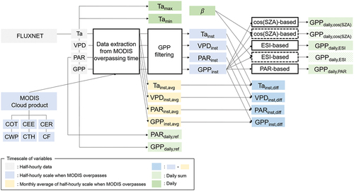The $f^{\prime }$ closely approximates $\mathit{f}$ as $\mathit{\beta }$ approaches 1 and has a smaller value than $\mathit{f}$ as $\mathit{\beta }$ approaches 0. The corrected temporal upscaling ratio was applied to GPP_inst and compared with the GPP_daily,ref. The overall data processing flow is depicted in Figure 1.

Figure 1. Flow diagram for key variables in this study. Different time scales are distinguished with box colors indicated at the bottom left. The box with dotted lines indicates the corrected temporal upscaling scheme.

4. Results and discussion

4.1. GPP_inst variation on the local overpassing time of MODIS in clear and cloudy conditions

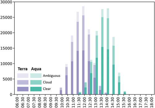
The ranges of the local overpassing time crossing the flux towers (Figure 2) were 10:00–14:00 for Terra-MODIS and 11:30–15:30 for Aqua-MODIS. The local times between 11:30–12:30 and 13:30–14:30 were the most frequent overpassing time of Terra and Aqua, respectively (Figure 2 and S1). A small difference in the local overpassing time between Terra and Aqua was observed on the flux towers at high latitudes above 55° (e.g. FI-Lom, FI-Hyy, and DK-Sor). The weather conditions during MODIS data collection are likely to be asymmetric in a day and can affect the result of temporal upscaling from instantaneous to daily-scale (Hu et al. 2018; Ryu et al. 2012). At the moments of MODIS data collection, cloudiness was observed in about 45% of the whole data. The probability of the existence of clouds over time was calculated for each site and is illustrated in Figure. S2. The latitudinal or longitudinal patterns of cloudiness with high probability were hard to find, but the frequency of cloudiness was generally higher in Aqua-MODIS than Terra-MODIS.

Figure 2. Histograms of the local overpass time for the terra-MODIS and aqua-MODIS. Histogram colors denote the cloudiness of the sky (i.e. clear, cloudy, and ambiguous) at its local overpass time. The cloudiness of the sky was distinguished based on the MODIS cloud mask product (i.e. MOD06 and MYD06).

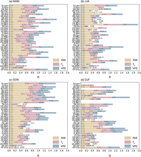
Atmospheric parameters change on a short-term scale, including clouds and aerosols, which influence surface solar radiation instantly (Xu et al. 2016). Variations in solar radiation can cause changes in other environmental variables, including temperature and humidity, through the exchange of force, momentum, energy, or mass (Jones 1985). Site-specific characteristics of the impact of microclimatic perturbations (i.e. PAR_inst,diff, Ta_inst,diff, and VPD_inst,diff) on GPP_inst,diff were analyzed in various biomes. Figure 3 depicts the seasonal correlation coefficients between GPP_inst,diff and each of PAR_inst,diff, Ta_inst,diff, and VPD_inst,diff. PAR_inst,diff generally showed moderate-to-strong positive relationships (R > 0.3) with GPP_inst,diff at most sites, regardless of the season. Some sites with DBF, CRO, and GRA had weak correlations between GPP_inst,diff and PAR_inst,diff (−0.3<R < 0.3) in winter because of the natural physiological processes, including litterfall. In contrast, Ta_inst,diff and VPD_inst,diff tend to present weak positive-to-negative correlations with GPP_inst,diff that coincide with the midday depression in photosynthesis due to high temperatures in mid-summer (Roessler and Monson 1985). Such site-specific GPP_inst,diff correlations with PAR_inst,diff, Ta_inst,diff, and VPD_inst,diff could vary because other environmental conditions, not considered in this paper, have the possibility to regulate plant photosynthesis. For instance, Gitelson et al. (2015) mentioned that the short-term photosynthetic activity responding to PAR could be affected by the long-term variation of phenological or physiological states, water treatment, and crop types. Plant photosynthesis in grasslands is also known to be the most sensitive to soil moisture (Baker, Denning, and Stöckli 2010; Flanagan, Wever, and Carlson 2002).

Figure 3. Site-level seasonal correlations between GPP_inst,diff with three environmental variables (PAR_inst,diff—yellow, Ta_inst,diff—red, VPD_inst,diff—blue). The correlation was calculated when the number of samples is larger than 10.

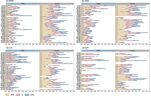
The different sky conditions revealed varied correlations between GPP_inst,diff and each of PAR_inst,diff, Ta_inst,diff, and VPD_inst,diff as shown in Figure 4. PAR_inst,diff is generally more correlated with GPP_inst,diff in the presence of clouds (R > 0.3) than in clear skies (−0.3 < R < 0.3), as the reduced PAR under cloudy conditions makes sunlit leaves less saturated (Tenhunen et al. 1984). Especially in summer, the study revealed that there were the weak-to-moderate negative correlations between GPP_inst,diff and Ta_inst,diff as well as VPD_inst,diff under clear skies, which was assumed to be attributed to the midday depression of photosynthesis (Grossiord et al. 2020; Yuan et al. 2019). In contrast, the weak positive correlations of GPP_inst,diff with Ta_inst,diff and VPD_inst,diff were observed under summer cloudy conditions. Changes in environmental interactions caused by clouds can weaken such negative correlations between GPP_inst,diff and Ta_inst,diff as well as VPD_inst,diff in summer. The relationship between GPP_inst,diff and VPD_inst,diff needs to be further explored in the future by separating temperature- or humidity-driven changes of VPD for various environmental conditions (Grossiord et al. 2020).

Figure 4. Site-level seasonal correlations between GPP_inst,diff with three environmental variables (PAR_inst,diff—yellow, Ta_inst,diff—red, VPD_inst,diff—blue) under clear and cloudy conditions. The correlation was calculated when the number of samples is larger than 10.

4.2. Temporal upscaling approaches on local overpassing time of MODIS under different skies

The half-hourly GPP values from the pre-processed data (refer to Section 3.1) were converted into daily-scale values using cos (SZA)-based, ESI-based, and PAR-based approaches. These values were then compared to the GPP_daily,ref values (refer to Section 3.2). The difference between GPP_daily,ref and the upscaled GPP values (i.e. GPP_{daily,cos (SZA)}, GPP_daily,ESI, and GPP_daily,PAR) varied by time. The GPP values upscaled with the GPP_inst obtained between 11 am and 1 pm yielded the best agreement with GPP_daily,ref, similar to Liu (2021). The slope and R² were closer to 1 compared to those for other times (Figures 5 and 6). After 11 am, the upscaled GPP values became increasingly underestimated in the cos (SZA)-based and ESI-based approaches over time compared to GPP_daily,ref. The slope reduced to 0.8, and RMSE and RRMSE increased up to about 1.2gC m⁻² d⁻¹ and 20%, respectively. It is noted that the PAR-based approach had a smaller decrease in slope between times than the cos (SZA)-based and ESI-based approaches, especially after 1 pm.

Figure 5. The station-based comparison of slope (refer to Section 3.2) between GPP_daily,ref and the upscaled GPP (i.e. blue: GPP_{daily,cos(SZA)}, purple: GPP_daily,ESI, yellow: GPP_daily,PAR) are presented according to vegetation types: (a) Deciduous broadleaf forests (DBF), (b) Evergreen broadleaf forests (EBF), (c) Evergreen needleleaf forests (ENF), (d) Mixed forests (MF), (e) Grasslands (GRA), and (f) Croplands (CRO). The comparison performed when the number of samples are larger than 10. The x-axis represents the local overpassing time of MODIS divided into one-hour intervals. The y-axis denotes the slope. The red dotted line shows where the slope is 1.

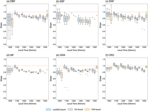
Figure 6. The station-based comparison of R² (referred to section 3.2) between GPP_daily,ref and the upscaled GPP (i.e. blue: GPP_{daily,cos(SZA)}, purple: GPP_daily,ESI, yellow: GPP_daily,PAR) are presented according to vegetation types: (a) deciduous broadleaf forests (DBF), (b) evergreen broadleaf forests (EBF), (c) evergreen needleleaf forests (ENF), (d) mixed forests (MF), (e) grasslands (GRA), and (f) croplands (CRO). The comparison performed when the number of samples are larger than 10. The x-axis represents the local overpassing time of MODIS divided into one-hour intervals. The y-axis denotes the R². The red dotted line shows where the R² is 1.

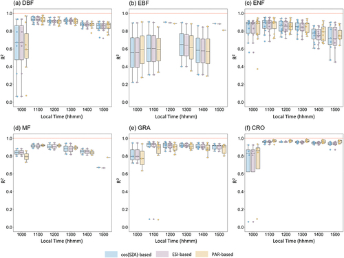
The upscaling factors of the cos (SZA)-based and ESI-based approaches sharply decreased after 1 pm, while the PAR-based approach had higher upscaling factors than others (Figure S5). A higher upscaling factor in the afternoon indicates a more flattened diurnal distribution (i.e. lower kurtosis) of incoming PAR, assuming that the diurnal incoming PAR distribution becomes symmetric around noon. The PAR-based approach seems better than other approaches as it reflects the diurnal changes of incoming PAR even in cloudy conditions. The result is consistent with Hu et al. (2018), who showed a more accurate prediction of daily GPP using the PAR-based approach than the cos (SZA)-based approach. Such a tendency is noticeable in the afternoon when cloudy conditions frequently occur (Figure S2). In particular, for the GF-Guy site, the correlation coefficient between the instantaneous-to-daily ratios of GPP and PAR was 0.5 for the PAR-based approach and 0.17 for the cos(SZA)-based and ESI-based approaches (not shown), indicating the PAR-based approach is more appropriate than others. On the other hand, the statistics for the three different temporal upscaling approaches between 10 am and 11 am showed the lowest values for slope and R² and the highest values for RMSE and RRMSE. Such results seem to come from the low GPP_inst values achieved in winter, which caused large deviations among the flux stations (Figures 5–6 and S3-S4).

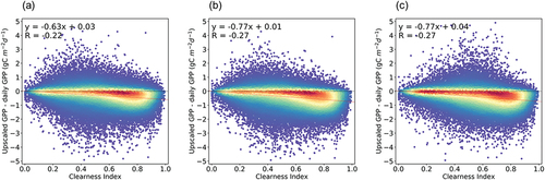
Figure 7 shows the comparisons between the clearness index and the difference between GPP_daily,ref and the upscaled GPP for three temporal upscaling approaches (refer to Section 3.4). The differences between GPP_daily,ref and the upscaled GPP values tended to be biased below zero as clearness index increased. With an increase in the clearness index, both air temperature and VPD also increased. These factors acted as limiting factors in plant photosynthesis, leading to an underestimation of the upscaled GPP values for all three approaches (Figure 7). Figure S6 depicts the relationships between the GPP_inst,diff and the difference between GPP_daily,ref and the upscaled GPP values. The cos (SZA)-based and ESI-based temporal upscaling approaches had weak positive correlations of 0.27 and 0.18, respectively, while the PAR-based temporal upscaling approach exhibited almost no correlation between them. It is noticeable that the PAR-based approach seems to better reflect the variance of instantaneous GPP compared to the cos (SZA)-based and ESI-based approaches. However, the PAR-based approach still exhibits a significant difference of about −5–5 gC m⁻² d⁻¹ when compared to GPP_daliy,ref, which is likely to be influenced by other environmental limiting factors such as air temperature and VPD.

Figure 7. The comparison between the clearness index and the difference between GPP_daily,ref and the three temporal upscaling approaches: (a) cos(SZA)-based, (b) ESI-based, (c) PAR-based. The red represents high point density while the blue indicates low point density.

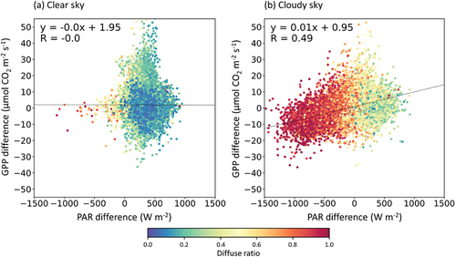
Whether diffuse radiation can enhance GPP in terrestrial ecosystems remains poorly understood (P. Liu et al. 2022). The amount of diffuse radiation is proportional to the total insolation and diffuse ratio, and the diffuse ratio varies aperiodically with clouds, aerosols, and atmospheric gases (e.g. water vapor, CO₂, O₃). The positive relationship between the diffuse ratio and GPP suggests that the light penetration of diffuse radiation into the canopy helps to enhance GPP. Figure S7 depicts the correlation coefficients between GPP_inst,diff and the diffuse ratio under clear and cloudy skies (refer to Section 3.3). Under clear sky conditions (PAR_inst,diff ≥0), the mean and standard deviation of the diffuse ratios were 0.23 and 0.12, respectively. Most eddy flux sites had weak positive correlations (R < 0.3), while DE-Hai and IT-PT1 exhibited moderate positive correlations (Figure S7). In contrast, the correlations between GPP_inst,diff and the diffuse ratio were slightly negative (R < −0.3) under cloudy sky conditions. PAR_inst,diff ranged from −343 W∙m⁻² to 200 W∙m⁻², and the mean and standard deviation of the diffuse ratios were 0.74 and 0.22, respectively. Only the CH-Oe1 site had a weak positive correlation whose GPP_inst,diff values were below zero in the cloudy condition. Such different correlations between GPP_inst,diff and the diffuse ratio under clear and cloudy conditions are further confirmed in Figure 8. In cloudy skies, as PAR_inst,diff decreased, GPP_inst,diff decreased, and the diffuse ratio tended to increase at the same time (Figure 8(b)), while no correlation was found in the clear skies (Figure 8(a)). High diffuse ratios above 0.5 tend to be distributed where PAR_inst,diff is below zero in Figure 8(b), which resulted in the negative correlations between GPP_inst,diff and the diffuse ratio. Such a trade-off between the increase in diffuse ratio and the reduced PAR can lead to a decrease in CO₂ uptake, as reported in previous studies (ALTON, NORTH, and LOS 2007; Kanniah et al. 2012). Our analysis demonstrated that the amount of changing PAR is more important than the diffuse ratio.

Figure 8. The relationships between GPP_inst,diff and PAR_inst,diff under (a) clear and (b) cloudy sky conditions. Colors indicate the diffuse ratio calculated from the eddy flux data.

4.3. Bias correction for cos (SZA)-based and ESI-based temporal upscaling approaches

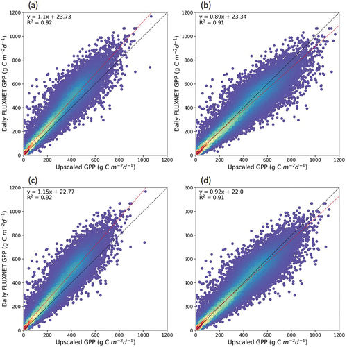
A GPP_inst, affected by ambient environmental conditions, including air temperature and VPD, as well as incoming solar radiation, leads it to underestimate the upscaled GPP on a daily scale. As incoming solar radiation is an influential factor for temporal upscaling, the PAR-based approach exhibited better performance across sites than the cos (SZA)-based and ESI-based approaches (Figure 5). Because the PAR-based approach requires spatially and temporally high-resolution PAR images with good quality regardless of weather conditions, the cos (SZA)-based and ESI-based approaches are more commonly used than the PAR-based approach. Therefore, we focused on correcting the underestimation of cos (SZA)-based and ESI-based approaches. The cos (SZA)-based and ESI-based approaches underestimated daily GPP in comparison with GPP_daily,ref (Figures. 9(a,c)). The corrected cos (SZA)-based and ESI-based temporal upscaling ratio $\mathit{f}{ }^{\mathrm{\prime }}$ (refer to section 3.5) slightly overestimated the GPP_daily,ref (Figures. 9(b-d)), but the RMSE after correction decreased by 10.69 and 21.07 gC m⁻² d⁻¹, respectively. However, in regions where the difference between daily maximum and minimum temperatures is small (e.g. GF-Guy), the correction effect was found to be smaller than at mid-latitude points.

Figure 9. Density plots between the upscaled daily GPP and reference data: (a) GPP_{cos (SZA),daily}, (b) corrected GPP_{cos (SZA),daily}, (c) GPP_ESI,daily, and (d) corrected GPP_ESI,daily.

4.4. Potential uncertainties in the temporal upscaling of satellite derived GPP products

MODIS onboard Terra and Aqua has various local overpassing times, as discussed in Section 4.1. The temporal difference between the input variables for modeling GPP_inst should be carefully considered because the performance of the temporal upscaling approaches was time-dependent (referred to in Section 4.2). The local overpassing time can be adjusted to some extent by reflecting the symmetrical pattern in the longtidue as shown in Figure S1. Meteorological variables are crucial for determining the time of the modeled GPP_inst because meteorological variables fluctuate on a short-time scale. Currently, reanalysis data is almost the only source that can provide meteorological variables on a sub-daily scale. Aggregating the modeled half-hourly GPP using reanalysis data could reflect the intricate plant photosynthesis on a global scale, but their spatial resolution is very low, ~ 0.5 degrees (Bonekamp, Collier, and Immerzeel 2018).

Meanwhile, temporal upscaling has the potential to convert the GPP_inst modeled using satellite-derived products at a higher spatial resolution (~1 km) to a daily scale. Our study showed that PAR-based temporal upscaling is more useful than other approaches under different sky conditions, which agrees with Hu et al. (2018). In reality, the PAR-based temporal upscaling could reflect different sky conditions, but the uncertainties of the modeled PAR_inst can exist. Recently, Li et al. (2021) estimated GPP_inst with fine spatial resolution at different times of the day using the land surface temperature derived from the Ecosystem Spaceborne Thermal Radiometer Experiment on the Space Station (i.e. ECOSTRESS). They concluded that the use of sub-daily meteorological data with a fine spatial resolution might further improve the daily GPP estimation. Considering the uncertainty in the daily sum of modeled GPP_inst, the temporal upscaling approaches (i.e. cos (SZA)-based and ESI-based) with the proposed correction on GPP_inst would be the best option except for tropical areas.

5. Conclusion

This study quantitatively analyzed temporal upscaling approaches from instantaneous to daily scale under different sky conditions and proposed a simple correction method using the difference between maximum and minimum temperatures in a day. The instantaneous GPP values of the FLUXNET2015 dataset on the MODIS overpassing time were transformed to the daily scale with three temporal upscaling approaches: cos (SZA)-based, ESI-based, and PAR-based ones. The local overpassing time of MODIS varied in the ranges of 10:00–14:00 for Terra-MODIS and 11:30–15:30 for Aqua-MODIS. It should be noted that about 45% of the data was collected in cloudy conditions. Among temporal upscaling approaches, the cos (SZA)-based and ESI-based approaches induced significant errors as the day progressed, with the reduced slope to 0.8 and the increased RMSE and RRMSE up to about 1.2gC m⁻² d⁻¹ and 20%, respectively. Conversely, the performance of the PAR-based approach remained remarkably stable over time, suggesting that it accurately captures the fluctuations in instantaneous GPP as influenced by clouds. The instant changes of PAR, Ta, and VPD generally had weak correlations with GPP under clear skies, while mid-to-high correlations were observed between the instant changes of GPP and PAR under cloudy conditions. At the daily scale, the three temporal upscaling approaches showed an overall underestimation over different clearness indices. To indirectly reflect the cloudy conditions over a day, we corrected cos (SZA)-based and ESI-based approaches by multiplying the correction factor using the difference of daily maximum-minimum air temperatures. The corrected upscaling factors reduced RMSE by 10.69 and 21.07 gC m⁻² d⁻¹ for the cos (SZA)-based and ESI-based approaches, respectively. In conclusion, for a global-scale satellite-based GPP model, aggregating the modeled GPP_inst would be the best way if the uncertainty is low. If not, universal temporal upscaling approaches (i.e. cos (SZA)-based and ESI-based) with the proposed correction factor would be an alternative. In future research, we will evaluate how well daily GPP, adjusted using the corrected temporal upscaling approach, responds to sudden meteorological disasters such as flash droughts or heavy rainfall events. This evaluation will contribute to understanding the resilience and accuracy of our GPP model in the face of unpredictable environmental changes.

Acknowledgments

We would like to express our sincere gratitude to Prof. Youngryel Ryu for providing valuable comments and insights during this research.

Disclosure statement

No potential conflict of interest was reported by the author(s).

Data availability statement

The FLUXNET2015 dataset is available at https://fluxnet.org/data/fluxnet2015-dataset/. The MODIS cloud products (i.e. MOD06_L2 and MYD06_L2) used in this study can be accessed through the NASA LAADS DAAC (https://ladsweb.modaps.eosdis.nasa.gov/search/).

Supplementary material

Supplemental data for this article can be accessed online at https://doi.org/10.1080/15481603.2024.2319372.

Additional information

Funding

This research was supported by Korea Environment Industry & Technology Institute (KEITI) through a project for developing an observation-based GHG emissions geospatial information map, funded by Korea Ministry of Environment (MOE) (RS-2023-00232066).

References

- Acosta, M., M. Pavelka, L. Montagnani, W. Kutsch, A. Lindroth, R. Juszczak, D. Janouš 2013. “Soil Surface CO2 Efflux Measurements in Norway Spruce Forests: Comparison Between Four Different Sites Across Europe - from Boreal to Alpine Forest.” Geoderma 192:295–19. https://doi.org/10.1016/j.geoderma.2012.08.027.
- Alton, P.B., P.R. North, S.O. Los 2007. “The Impact of Diffuse Sunlight on Canopy Light-Use Efficiency, Gross Photosynthetic Product and Net Ecosystem Exchange in Three Forest Biomes.” Global Change Biology 13 (4): 776–787. https://doi.org/10.1111/j.1365-2486.2007.01316.x.
- Ammann, C., C. Spirig, J. Leifeld, and A. Neftel. 2009. “Assessment of the Nitrogen and Carbon Budget of Two Managed Temperate Grassland Fields.” Agriculture, Ecosystems & Environment 133 (3–4): 150–162. https://doi.org/10.1016/j.agee.2009.05.006.
- Anthoni, P.M., A. Knohl, C. Rebmann, A. Freibauer, M. Mund, W. Mund, O. Mund, E.-D. Schulze 2004. “Forest and Agricultural Land-Use-Dependent CO 2 Exchange in Thuringia, Germany.” Global Change Biology 10 (12): 2005–2019. https://doi.org/10.1111/j.1365-2486.2004.00863.x.
- Aurela, M., L. Annalea, J.-P. Tuovinen, J. Hatakka, T. Penttilä, T. Laurila 2015. “Carbon Dioxide and Energy Flux Measurements in Four Northern-Boreal Ecosystems at Pallas.” Boreal Environment Research 20 (4): 455–473. https://www.borenv.net/BER/archive/ber204.htm.
- Baker, I.T., A.S, Denning, R. Stöckli 2010. “North American Gross Primary Productivity: Regional Characterization and Interannual Variability.” Tellus B Chemical and Physical Meteorology 62 (5): 533–549. https://doi.org/10.1111/j.1600-0889.2010.00492.x.
- Baldocchi, D., E. Falge, L. Gu, R. Olson, D. Hollinger, S. Running, P. Anthoni, C. Bernhofer, K. Davis, R. Evans, J. Fuentes, A. Goldstein, G. Katul, B. Law, X. Lee, Y. Malhi, T. Meyers, W. Munger, W. Oechel, U.K.T., Paw, K. H.P. Pilegaard, Schmid, R. Valentini, S. Verma, T. Vesala, K. Wilson, S. Wofsy 2001. “FLUXNET: A New Tool to Study the Temporal and Spatial Variability of Ecosystem–Scale Carbon Dioxide, Water Vapor, and Energy Flux Densities.” Bulletin of the American Meteorological Society 82 (11): 2415–2434. 200182<2415:FANTTS>2.3.CO;2. https://doi.org/10.1175/1520-0477(2001)082<2415:FANTTS>2.3.CO;2.
- Berbigier, P., J. M. Bonnefond, and P. Mellmann. 2001. “CO2 and Water Vapour Fluxes for 2 Years Above Euroflux Forest Site.” Agricultural and Forest Meteorology 108 (3): 183–197. https://doi.org/10.1016/S0168-1923(01)00240-4.
- Bonal, D., Bosc, A., Ponton, S., Goret, J.-Y., Burban, B., Gross, P., Bonnefond, J.-M., Elbers, J., Longdoz, B., Epron, D., Guehl, J.-M., Granier, A. 2008. “Impact of Severe Dry Season on Net Ecosystem Exchange in the Neotropical Rainforest of French Guiana.” Global Change Biology 14 (8): 1917–1933. https://doi.org/10.1111/j.1365-2486.2008.01610.x.
- Bonekamp, P. N. J., E. Collier, and W. Immerzeel. 2018. “The Impact of Spatial Resolution, Land Use, and Spinup Time on Resolving Spatial Precipitation Patterns in the Himalayas.” Journal of Hydrometeorology 19 (10): 1565–1581. https://doi.org/10.1175/JHM-D-17-0212.1.
- Chen, S., Liu, L., He, X., Liu, Z., Peng, D. 2020. “Upscaling from Instantaneous to Daily Fraction of Absorbed Photosynthetically Active Radiation (FAPAR) for Satellite Products.” Remote Sensing 12 (13): 2083. 2083. https://doi.org/10.3390/rs12132083.
- Chiesi, M., F. Maselli, M. Bindi, L. Fibbi, P. Cherubini, E. Arlotta, G. Tirone, G. Matteucci, and G. Seufert. 2005. “Modelling Carbon Budget of Mediterranean Forests Using Ground and Remote Sensing Measurements.” Agricultural and Forest Meteorology 135 (1–4): 22–34. https://doi.org/10.1016/j.agrformet.2005.09.011.
- Cirino, G. G., R. A. F. Souza, D. K. Adams, and P. Artaxo. 2014. “The Effect of Atmospheric Aerosol Particles and Clouds on Net Ecosystem Exchange in the Amazon.” Atmospheric Chemistry & Physics 14 (13): 6523–6543. https://doi.org/10.5194/acp-14-6523-2014.
- Cook, B. D., K. J. Davis, W. Wang, A. Desai, B. W. Berger, R. M. Teclaw, J. G. Martin, et al. 2004. “Carbon Exchange and Venting Anomalies in an Upland Deciduous Forest in Northern Wisconsin, USA.” Agricultural and Forest Meteorology 126 (3–4): 271–295. https://doi.org/10.1016/j.agrformet.2004.06.008.
- Curtis, P. S., P. J. Hanson, P. Bolstad, C. Barford, J. C. Randolph, H. P. Schmid, and K. B. Wilson. 2002. “Biometric and Eddy-Covariance Based Estimates of Annual Carbon Storage in Five Eastern North American Deciduous Forests.” Agricultural and Forest Meteorology 113 (1–4): 3–19. https://doi.org/10.1016/S0168-1923(02)00099-0.
- Desai, A. R., A. Noormets, P. V. Bolstad, J. Chen, B. D. Cook, K. J. Davis, E. S. Euskirchen, et al. 2008. “Influence of Vegetation and Seasonal Forcing on Carbon Dioxide Fluxes Across the Upper Midwest, USA: Implications for Regional Scaling.” Agricultural and Forest Meteorology 148 (2): 288–308. https://doi.org/10.1016/j.agrformet.2007.08.001.
- Dietiker, D., N. Buchmann, and W. Eugster. 2010. “Testing the Ability of the DNDC Model to Predict CO2 and Water Vapour Fluxes of a Swiss Cropland Site.” Agriculture, Ecosystems & Environment 139 (3): 396–401. https://doi.org/10.1016/j.agee.2010.09.002.
- Dragoni, D., H. P. Schmid, C. S. B. Grimmond, and H. W. Loescher. 2007. “Uncertainty of Annual Net Ecosystem Productivity Estimated Using Eddy Covariance Flux Measurements.” Journal of Geophysical Research: Atmospheres 112 (D17): D17102. https://doi.org/10.1029/2006JD008149.
- Feng, Y., Chen, D., Zhao, X. 2020. “Impact of Aerosols on Terrestrial Gross Primary Productivity in North China Using an Improved Boreal Ecosystem Productivity Simulator with Satellite-Based Aerosol Optical Depth.” GIScience & Remote Sens 57 (2): 258–270. https://doi.org/10.1080/15481603.2019.1682237.
- Flanagan, L.B., Wever, L.A., Carlson, P.J. 2002. “Seasonal and Interannual Variation in Carbon Dioxide Exchange and Carbon Balance in a Northern Temperate Grassland.” Global Change Biology 8 (7): 599–615. https://doi.org/10.1046/j.1365-2486.2002.00491.x.
- Free, M., B. Sun, and H. L. Yoo. 2016. “Comparison Between Total Cloud Cover in Four Reanalysis Products and Cloud Measured by Visual Observations at U.S. Weather Stations.” Journal of Climate 29 (6): 2015–2021. https://doi.org/10.1175/JCLI-D-15-0637.1.
- Gilabert, M. A., A. Moreno, F. Maselli, B. Martínez, M. Chiesi, S. Sánchez-Ruiz, F. J. García-Haro, et al. 2015. “Daily GPP Estimates in Mediterranean Ecosystems by Combining Remote Sensing and Meteorological Data.” ISPRS Journal of Photogrammetry and Remote Sensing 102:184–197. https://doi.org/10.1016/j.isprsjprs.2015.01.017.
- Gitelson, A. A., Y. Peng, T. J. Arkebauer, and A. E. Suyker. 2015. “Productivity, Absorbed Photosynthetically Active Radiation, and Light Use Efficiency in Crops: Implications for Remote Sensing of Crop Primary Production.” Journal of Plant Physiology 177:100–109. https://doi.org/10.1016/j.jplph.2014.12.015.
- Goodrich, J.P., Campbell, D.I., Clearwater, M.J., Rutledge, S., Schipper, L.A. 2015. “High Vapor Pressure Deficit Constrains GPP and the Light Response of NEE at a Southern Hemisphere Bog.” Agricultural and Forest Meteorology 203:112–123. https://doi.org/10.1016/j.agrformet.2015.01.001.
- Green, C., and Byrne, K.A. 2004. ”Impact on Carbon Cycle and Greenhouse Gas Emissions.” In Encyclopedia of energyyear, 223–236. Amsterdam, Boston: Elsevier Academic Press. https://doi.org/10.1016/b0-12-176480-x/00418-6.
- Grossiord, C., Buckley, T.N., Cernusak, L.A., Novick, K.A., Poulter, B., Siegwolf, R.T.W., Sperry, J.S., McDowell, N.G. 2020. “Plant responses to rising vapor pressure deficit.” The New Phytologist 226 (6): 1550–1566. https://doi.org/10.1111/nph.16485.
- Grünwald, T., Bernhofer, C. 2007. “A Decade of Carbon, Water and Energy Flux Measurements of an Old Spruce Forest at the Anchor Station Tharandt.”in Tellus, Series B: Chemical and Physical Meteorology 59 (3): 387–396. https://doi.org/10.1111/j.1600-0889.2007.00259.x.
- Hao, D., G. R. Asrar, Y. Zeng, Q. Zhu, J. Wen, Q. Xiao, and M. Chen. 2019. “Estimating Hourly Land Surface Downward Shortwave and Photosynthetically Active Radiation from DSCOVR/EPIC Observations.” Remote Sensing of Environment 232:111320. https://doi.org/10.1016/j.rse.2019.111320.
- Hollinger, D. Y., and A. D. Richardson. 2005. “Uncertainty in Eddy Covariance Measurements and Its Application to Physiological Models.” Tree Physiology 25 (7): 873–885. https://doi.org/10.1093/treephys/25.7.873.
- Huang, Y., A. Bárdossy, and K. Zhang. 2019. “Sensitivity of Hydrological Models to Temporal and Spatial Resolutions of Rainfall Data.” Hydrology and Earth System Sciences 23 (6): 2647–2663. https://doi.org/10.5194/hess-23-2647-2019.
- Hu, J., L. Liu, J. Guo, S. Du, and X. Liu. 2018. “Upscaling Solar-Induced Chlorophyll Fluorescence from an Instantaneous to Daily Scale Gives an Improved Estimation of the Gross Primary Productivity.” Remote Sensing 10 (10): 1663. https://doi.org/10.3390/rs10101663.
- Jiang, C., K. Guan, G. Wu, B. Peng, and S. Wang. 2021. “A Daily, 250 M and Real-Time Gross Primary Productivity Product (2000–Present) Covering the Contiguous United States.” Earth System Science Data 13 (2): 281–298. https://doi.org/10.5194/essd-13-281-2021.
- Jiang, C., Ryu, Y. 2016. “Multi-Scale Evaluation of Global Gross Primary Productivity and Evapotranspiration Products Derived from Breathing Earth System Simulator (BESS). Remote Sens.” Remote Sensing of Environment 186:528–547. https://doi.org/10.1016/j.rse.2016.08.030.
- Jiang, S., C. Zhao, and Y. Xia. 2022. “Distinct Response of Near Surface Air Temperature to Clouds in North China.” Atmospheric Science Letters 23 (12): e1128. https://doi.org/10.1002/asl.1128.
- Joiner, J., and Y. Yoshida. 2020. “Satellite-Based Reflectances Capture Large Fraction of Variability in Global Gross Primary Production (GPP) at Weekly Time Scales.” Agricultural and Forest Meteorology 291:108092. https://doi.org/10.1016/j.agrformet.2020.108092.
- Jones, M.B. 1985. “Plant microclimate.” In Techniques in Bioproductivity and Photosynthesis, 26–40. Elsevier. https://doi.org/10.1016/B978-0-08-031999-5.50013-3.
- Jung, M., Reichstein, M., Bondeau, A. 2009. “Towards Global Empirical Upscaling of FLUXNET Eddy Covariance Observations: Validation of a Model Tree Ensemble Approach Using a Biosphere Model.” Biogeosciences 6 (10): 2001–2013. https://doi.org/10.5194/bg-6-2001-2009.
- Jung, M., M. Vetter, M. Herold, G. Churkina, M. Reichstein, S. Zaehle, P. Ciais, et al. 2007. “Uncertainties of Modeling Gross Primary Productivity Over Europe: A Systematic Study on the Effects of Using Different Drivers and Terrestrial Biosphere Models.” Global Biogeochemical Cycles 21 (4): n/a–n/a. https://doi.org/10.1029/2006GB002915.
- Kaiser, E., Morales, A., Harbinson, J., Kromdijk, J., Heuvelink, E., Marcelis, L.F.M. 2015. “Dynamic Photosynthesis in Different Environmental Conditions.” Journal of Experimental Botany 66 (9): 2415–2426. https://doi.org/10.1093/jxb/eru406.
- Kanniah, K. D., J. Beringer, P. North, and L. Hutley. 2012. “Control of Atmospheric Particles on Diffuse Radiation and Terrestrial Plant Productivity: A Review.” Progress in Physical Geography: Earth and Environment 36 (2): 209–237. https://doi.org/10.1177/0309133311434244.
- Knohl, A., E. D. Schulze, O. Kolle, and N. Buchmann. 2003. “Large Carbon Uptake by an Unmanaged 250-Year-Old Deciduous Forest in Central Germany.” Agricultural and Forest Meteorology 118 (3–4): 151–167. https://doi.org/10.1016/S0168-1923(03)00115-1.
- LASSLOP, G., REICHSTEIN, M., PAPALE, D., RICHARDSON, A.D., ARNETH, A., BARR, A., STOY, P., WOHLFAHRT, G. 2010. “Separation of net ecosystem exchange into assimilation and respiration using a light response curve approach: critical issues and global evaluation.” Global Change Biology 16 (1): 187–208. https://doi.org/10.1111/j.1365-2486.2009.02041.x.
- L’Ecuyer, T. S., Y. Hang, A. V. Matus, and Z. Wang. 2019. “Reassessing the Effect of Cloud Type on Earth’s Energy Balance in the Age of Active Spaceborne Observations. Part I: Top of Atmosphere and Surface.” Journal of Climate 32 (19): 6197–6217. https://doi.org/10.1175/JCLI-D-18-0753.1.
- Liu, Z. 2021. “The Accuracy of Temporal Upscaling of Instantaneous Evapotranspiration to Daily Values with Seven Upscaling Methods.” Hydrology and Earth System Sciences 25 (8): 4417–4433. https://doi.org/10.5194/hess-25-4417-2021.
- Liu, P., X. Tong, J. Zhang, P. Meng, J. Li, J. Zhang, and Y. Zhou. 2022. “Effect of Diffuse Fraction on Gross Primary Productivity and Light Use Efficiency in a Warm-Temperate Mixed Plantation.” Frontiers in Plant Science 13:966125. https://doi.org/10.3389/fpls.2022.966125.
- Li, X., J. Xiao, J. B. Fisher, and D. D. Baldocchi. 2021. “ECOSTRESS Estimates Gross Primary Production with Fine Spatial Resolution for Different Times of Day from the International Space Station.” Remote Sensing of Environment 258:112360. https://doi.org/10.1016/j.rse.2021.112360.
- Li, L., X. Xin, H. Zhang, J. Yu, Q. Liu, S. Yu, and J. Wen. 2015. “A Method for Estimating Hourly Photosynthetically Active Radiation (PAR) in China by Combining Geostationary and Polar-Orbiting Satellite Data.” Remote Sensing of Environment 165:14–26. https://doi.org/10.1016/j.rse.2015.03.034.
- Li, Z., G. Yu, X. Xiao, Y. Li, X. Zhao, C. Ren, L. Zhang, and Y. Fu. 2007. “Modeling Gross Primary Production of Alpine Ecosystems in the Tibetan Plateau Using MODIS Images and Climate Data.” Remote Sensing of Environment 107 (3): 510–519. https://doi.org/10.1016/j.rse.2006.10.003.
- Mäkelä, A., P. Kolari, J. Karimäki, E. Nikinmaa, M. Perämäki, and P. Hari. 2006. “Modelling Five Years of Weather-Driven Variation of GPP in a Boreal Forest.” Agricultural and Forest Meteorology 139 (3–4): 382–398. https://doi.org/10.1016/j.agrformet.2006.08.017.
- Marchesini, L.B., Papale, D., Reichstein, M., Vuichard, N., Tchebakova, N., Valentini, R. 2007. “Carbon Balance Assessment of a Natural Steppe of Southern Siberia by Multiple Constraint Approach.” Biogeosciences 4 (4): 581–595. https://doi.org/10.5194/bg-4-581-2007.
- Marcolla, B., A. Cescatti, G. Manca, R. Zorer, M. Cavagna, A. Fiora, D. Gianelle, M. Rodeghiero, M. Sottocornola, and R. Zampedri. 2011. “Climatic Controls and Ecosystem Responses Drive the Inter-Annual Variability of the Net Ecosystem Exchange of an Alpine Meadow.” Agricultural and Forest Meteorology 151 (9): 1233–1243. https://doi.org/10.1016/j.agrformet.2011.04.015.
- Mengistu, A.G., Mengistu Tsidu, G., Koren, G., Kooreman, M., Boersma, K.F., Tagesson, T., Ardö, J., Nouvellon, Y., Peters, W. 2020. “Sun-Induced Fluorescence and Near Infrared Reflectance of Vegetation Track the Seasonal Dynamics of Gross Primary Production Over Africa.” Biogeosciences Discuss 1–23. https://doi.org/10.5194/bg-2020-242.
- Miao, G., Guan, K., Yang, X., Bernacchi, C.J., Berry, J.A., DeLucia, E.H., Wu, J., Moore, C.E., Meacham, K., Cai, Y., Peng, B., Kimm, H., Masters, M.D. 2018. “Sun-Induced Chlorophyll Fluorescence, Photosynthesis, and Light Use Efficiency of a Soybean Field from Seasonally Continuous Measurements.” Journal of Geophysical Research-Biogeosciences 123 (2): 610–623. https://doi.org/10.1002/2017JG004180.
- Migliavacca, M., Meroni, M., Busetto, L., Colombo, R., Zenone, T., Matteucci, G., Manca, G., Seufert, G. 2009. “Modeling Gross Primary Production of Agro-Forestry Ecosystems by Assimilation of Satellite-Derived Information in a Process-Based Model.” Sensors 9 (2): 922–942. https://doi.org/10.3390/s90200922.
- Montagnani, L., G. Manca, E. Canepa, E. Georgieva, M. Acosta, C. Feigenwinter, D. Janous, et al. 2009. “A New Mass Conservation Approach to the Study of CO2 Advection in an Alpine Forest.” Journal of Geophysical Research: Atmospheres 114 (D7): 7306. https://doi.org/10.1029/2008JD010650.
- Moors, E.J. 2012. Water Use of Forests in the Netherlands. PhD diss., Vrije Universiteit Amsterdam.
- Park, H., J. Im, and M. Kim. 2019. “Improvement of Satellite-Based Estimation of Gross Primary Production Through Optimization of Meteorological Parameters and High Resolution Land Cover Information at Regional Scale Over East Asia.” Agricultural and Forest Meteorology 271:180–192. https://doi.org/10.1016/j.agrformet.2019.02.040.
- Pastorello, G., Trotta, C., Canfora, E., Chu, H., Christianson, D., Cheah, Y.W., Poindexter, C., Chen, J., Elbashandy, A., Humphrey, M., et al. 2020. “The FLUXNET2015 Dataset and the ONEFlux Processing Pipeline for Eddy Covariance Data.” Sci., 225. 7. https://doi.org/10.1038/s41597-020-0534-3.
- Pilegaard, K., A. Ibrom, M. S. Courtney, P. Hummelshøj, and N. O. Jensen. 2011. “Increasing Net CO2 Uptake by a Danish Beech Forest During the Period from 1996 to 2009.” Agricultural and Forest Meteorology 151 (7): 934–946. https://doi.org/10.1016/j.agrformet.2011.02.013.
- Pinker, R.T., Laszlo, I. 1992. “Global Distribution of Photosynthetically Active Radiation as Observed from Satellites.” Journal of Climate 5 (1): 56–65. https://doi.org/10.1175/1520-0442(1992)005<0056:GDOPAR>2.0.CO;2.
- Qiu, B., Yan, X., Chen, C., Tang, Z., Wu, W., Xu, W., Zhao, Z., Yan, C., Berry, J., Huang, W., et al. 2021. “The Impact of Indicator Selection on Assessment of Global Greening.” GIScience & Remote Sensing 58 (3): 372–385. https://doi.org/10.1080/15481603.2021.1879494.
- Rambal, S., Joffre, R., Ourcival, J.M., Cavender-Bares, J., Rocheteau, A. 2004. “The Growth Respiration Component in Eddy CO 2 Flux from a Quercus Ilex Mediterranean Forest.” Global Change Biology 10 (9): 1460–1469. https://doi.org/10.1111/j.1365-2486.2004.00819.x.
- Rascher, U., and L. Nedbal. 2006. “Dynamics of Photosynthesis in Fluctuating Light.” Current Opinion in Plant Biology 9 (6): 671–678. https://doi.org/10.1016/j.pbi.2006.09.012.
- Reichstein, M., Falge, E., Baldocchi, D., Papale, D., Aubinet, M., Berbigier, P., Bernhofer, C., Buchmann, N., Gilmanov, T., Granier, A., Grunwald, T., Havrankova, K., Ilvesniemi, H., Janous, D., Knohl, A., Laurila, T., Lohila, A., Loustau, D., Matteucci, G., Meyers, T., Miglietta, F., Ourcival, J.-M., Pumpanen, J., Rambal, S., Rotenberg, E., Sanz, M., Tenhunen, J., Seufert, G., Vaccari, F., Vesala, T., Yakir, D., Valentini, R. 2005. “On the Separation of Net Ecosystem Exchange into Assimilation and Ecosystem Respiration: Review and Improved Algorithm.” Global Change Biology 11 (9): 1424–1439. https://doi.org/10.1111/j.1365-2486.2005.001002.x.
- Roessler, P.G., Monson, R.K. 1985. “Midday Depression in Net Photosynthesis and Stomatal Conductance in Yucca glauca - Relative Contributions of Leaf Temperature and Leaf-To-Air Water Vapor Concentration Difference.” Oecologia 67 (3): 380–387. https://doi.org/10.1007/BF00384944.
- Running, S.W., Nemani, R.R., Heinsch, F.A., Zhao, M., Reeves, M., Hashimoto, H. 2004. A Continuous Satellite-Derived Measure of Global Terrestrial Primary Production, BioScience. Oxford Academic. https://doi.org/10.1641/0006-3568.
- Ryu, Y., D. D. Baldocchi, T. A. Black, M. Detto, B. E. Law, R. Leuning, A. Miyata, et al. 2012. “On the Temporal Upscaling of Evapotranspiration from Instantaneous Remote Sensing Measurements to 8-Day Mean Daily-Sums.” Agricultural and Forest Meteorology 152:212–222. https://doi.org/10.1016/j.agrformet.2011.09.010.
- Ryu, Y., Baldocchi, D.D., Kobayashi, H., Van Ingen, C., Li, J., Black, T.A., Beringer, J., Van Gorsel, E., Knohl, A., Law, B.E., Roupsard, O. 2011. “Integration of MODIS Land and Atmosphere Products with a Coupled-Process Model to Estimate Gross Primary Productivity and Evapotranspiration from 1 Km to Global Scales.” Global Biogeochemical Cycles 25 (4): Cycles 25. https://doi.org/10.1029/2011GB004053.
- Ryu, Y., D. D. Baldocchi, S. Ma, and T. Hehn. 2008. “Interannual Variability of Evapotranspiration and Energy Exchange Over an Annual Grassland in California.” Journal of Geophysical Research: Atmospheres 113 (D9): D09104. https://doi.org/10.1029/2007JD009263.
- Ryu, Y., J. A. Berry, and D. D. Baldocchi. 2019. “What is Global Photosynthesis? History, Uncertainties and Opportunities.” Remote Sensing of Environment 223:95–114. https://doi.org/10.1016/j.rse.2019.01.016.
- Sasai, T., Ichii, K., Yamaguchi, Y., Nemani, R. 2005. “Simulating Terrestrial Carbon Fluxes Using the New Biosphere Model “Biosphere Model Integrating Eco-Physiological and Mechanistic Approaches Using Satellite data” (BEAMS).” Journal of Geophysical Research Biogeosciences 110 (G2): n/a–n/a. https://doi.org/10.1029/2005JG000045.
- Suni, T., Rinne, J., Reissell, A., Altimir, N., Keronen, P., Rannik, Ü., Dal Maso, M., Kulmala, M., Vesala, T. 2003. “Long-Term Measurements of Surface Fluxes Above a Scots Pine Forest in Hyytiälä, Southern Finland, 1996-2001.” Boreal Environment Research 8 (4): 287–301. https://www.borenv.net/BER/archive/ber84.htm.
- Sun, Y., Peng, D., Guan, X., Chu, D., Ma, Y., Shen, H. 2023. “Impacts of the Data Quality of Remote Sensing Vegetation Index on Gross Primary Productivity Estimation.” GIScience & Remote Sensing 60 (1): 2275421. https://doi.org/10.1080/15481603.2023.2275421.
- Suyker, A. E., S. B. Verma, G. G. Burba, and T. J. Arkebauer. 2005. “Gross Primary Production and Ecosystem Respiration of Irrigated Maize and Irrigated Soybean During a Growing Season.” Agricultural and Forest Meteorology 131 (3–4): 180–190. https://doi.org/10.1016/j.agrformet.2005.05.007.
- Tagliabue, G., C. Panigada, B. Dechant, F. Baret, S. Cogliati, R. Colombo, M. Migliavacca, et al. 2019. “Exploring the Spatial Relationship Between Airborne-Derived Red and Far-Red Sun-Induced Fluorescence and Process-Based GPP Estimates in a Forest Ecosystem.” Remote Sensing of Environment 231:111272. https://doi.org/10.1016/j.rse.2019.111272.
- TEDESCHI, V., REY, A., MANCA, G., VALENTINI, R., JARVIS, P.G., BORGHETTI, M. 2006. “Soil Respiration in a Mediterranean Oak Forest at Different Developmental Stages After Coppicing.” Global Change Biology 12 (1): 110–121. https://doi.org/10.1111/j.1365-2486.2005.01081.x.
- Tenhunen, J.D., Lange, O.L., Gebel, J., Beyschlag, W., Weber, J.A. 1984. “Changes in Photosynthetic Capacity, Carboxylation Efficiency, and CO2 Compensation Point Associated with Midday Stomatal Closure and Midday Depression of Net CO2 Exchange of Leaves of Quercus Suber.” Planta 162 (3): 193–203. https://doi.org/10.1007/BF00397440.
- Thomas, C. K., B. E. Law, J. Irvine, J. G. Martin, J. C. Pettijohn, and K. J. Davis. 2009. “Seasonal Hydrology Explains Interannual and Seasonal Variation in Carbon and Water Exchange in a Semiarid Mature Ponderosa Pine Forest in Central Oregon.” Journal of Geophysical Research: Atmospheres 114 (G4): G04006. https://doi.org/10.1029/2009JG001010.
- Tramontana, G., Jung, M., Schwalm, C.R., Ichii, K., Camps-Valls, G., Ráduly, B., Reichstein, M., Arain, M.A., Cescatti, A., Kiely, G., Merbold, L., Serrano-Ortiz, P., Sickert, S., Wolf, S., Papale, D. 2016. “Predicting Carbon Dioxide and Energy Fluxes Across Global FLUXNET Sites with Regression Algorithms.” Biogeosciences 13 (14): 4291–4313. https://doi.org/10.5194/bg-13-4291-2016.
- Tramontana, G., Migliavacca, M., Jung, M., Reichstein, M., Keenan, T.F., Camps-Valls, G., Ogee, J., Verrelst, J., Papale, D. 2020. “Partitioning net carbon dioxide fluxes into photosynthesis and respiration using neural networks.” Global Change Biology 26 (9): 5235–5253. https://doi.org/10.1111/gcb.15203.
- VALENTINI, R., ANGELIS, P., MATTEUCCI, G., MONACO, R., DORE, S., MUCNOZZA, G.E.S. 1996. “Seasonal Net Carbon Dioxide Exchange of a Beech Forest with the Atmosphere.” Global Change Biology 2 (3): 199–207. https://doi.org/10.1111/j.1365-2486.1996.tb00072.x.
- Vitale, L., P. Di Tommasi, G. D’Urso, and V. Magliulo. 2016. “The Response of Ecosystem Carbon Fluxes to LAI and Environmental Drivers in a Maize Crop Grown in Two Contrasting Seasons.” International Journal of Biometeorology 60 (3): 411–420. https://doi.org/10.1007/s00484-015-1038-2.
- Walther, S., Guanter, L., Heim, B., Jung, M., Duveiller, G., Wolanin, A., Sachs, T. 2018. “Assessing the Dynamics of Vegetation Productivity in Circumpolar Regions with Different Satellite Indicators of Greenness and Photosynthesis.” Biogeosciences 15 (20): 6221–6256. https://doi.org/10.5194/bg-15-6221-2018.
- Wang, F., Gonsamo, A., Chen, J.M., Black, T.A., Zhou, B. 2014. “Instantaneous-To-Daily GPP Upscaling Schemes Based on a Coupled Photosynthesis-Stomatal Conductance Model: Correcting the Overestimation of GPP by Directly Using Daily Average Meteorological Inputs.” Oecologia 176 (3): 703–714. https://doi.org/10.1007/s00442-014-3059-7.
- Way, D.A., Pearcy, R.W. 2012. Sunflecks in Trees and Forests: From Photosynthetic Physiology to Global Change Biology. Tree Physiol. 32(9): 1066-1081. https://doi.org/10.1093/treephys/tps064.
- Wohlfahrt, G., A. Hammerle, A. Haslwanter, M. Bahn, U. Tappeiner, and A. Cernusca. 2008. “Seasonal and Inter-Annual Variability of the Net Ecosystem CO 2 Exchange of a Temperate Mountain Grassland: Effects of Weather and Management.” Journal of Geophysical Research: Atmospheres 113 (D8): D08110. https://doi.org/10.1029/2007JD009286.
- Xiao, J., F. Chevallier, C. Gomez, L. Guanter, J. A. Hicke, A. R. Huete, K. Ichii, et al. 2019. “Remote Sensing of the Terrestrial Carbon Cycle: A Review of Advances Over 50 Years.” Remote Sensing of Environment 233:111383. https://doi.org/10.1016/j.rse.2019.111383.
- Xiao, X., Zhang, Q., Braswell, B., Urbanski, S., Boles, S., Wofsy, S., Moore, B., Ojima, D. 2004. “Modeling gross primary production of temperate deciduous broadleaf forest using satellite images and climate data.” Remote Sensing of Environment 91 (2): 256–270. https://doi.org/10.1016/j.rse.2004.03.010.
- Xie, X., A. Li, J. Tan, H. Jin, X. Nan, Z. Zhang, J. Bian, and G. Lei. 2020. “Assessments of Gross Primary Productivity Estimations with Satellite Data-Driven Models Using Eddy Covariance Observation Sites Over the Northern Hemisphere.” Agricultural and Forest Meteorology 280:107771. https://doi.org/10.1016/j.agrformet.2019.107771.
- Xu, H., J. Guo, X. Ceamanos, J. L. Roujean, M. Min, and D. Carrer. 2016. “On the Influence of the Diurnal Variations of Aerosol Content to Estimate Direct Aerosol Radiative Forcing Using MODIS Data.” Atmospheric Environment 141:186–196. https://doi.org/10.1016/j.atmosenv.2016.06.067.
- Yang, F., K. Ichii, M. A. White, H. Hashimoto, A. R. Michaelis, P. Votava, A. X. Zhu, A. Huete, S. W. Running, and R. R. Nemani. 2007. “Developing a Continental-Scale Measure of Gross Primary Production by Combining MODIS and AmeriFlux Data Through Support Vector Machine Approach.” Remote Sensing of Environment 110 (1): 109–122. https://doi.org/10.1016/j.rse.2007.02.016.
- Yao, B., C. Liu, Y. Yin, Z. Liu, C. Shi, H. Iwabuchi, and F. Weng. 2020. “Evaluation of Cloud Properties from Reanalyses Over East Asia with a Radiance-Based Approach.” Atmospheric Measurement Techniques 13 (3): 1033–1049. https://doi.org/10.5194/amt-13-1033-2020.
- Yuan, W., Zheng, Y., Piao, S., Ciais, P., Lombardozzi, D., Wang, Y., Ryu, Y., Chen, G., Dong, W., Hu, Z., Jain, A.K., Jiang, C., Kato, E., Li, S., Lienert, S., Liu, S., Nabel, J.E.M.S., Qin, Z., Quine, T., Sitch, S., Smith, W.K., Wang, F., Wu, C., Xiao, Z., Yang, S. 2019. “Increased Atmospheric Vapor Pressure Deficit Reduces Global Vegetation Growth.” Science Advances 5 (8): eaax1396. https://doi.org/10.1126/sciadv.aax1396.
- Zhang, X., N. Lu, H. Jiang, and L. Yao. 2020. “Evaluation of Reanalysis Surface Incident Solar Radiation Data in China.” Scientific Reports 10 (1): 1–20. https://doi.org/10.1038/s41598-020-60460-1.
- Zhang, W., Luo, G., Hamdi, R., Ma, X., Li, Y., Yuan, X., Li, C., Ling, Q., Hellwich, O., Termonia, P., et al. 2023. “Can Gross Primary Productivity Products Be Effectively Evaluated in Regions with Few Observation Data?” GIScience & Remote Sensing 60 (1): 2213489. https://doi.org/10.1080/15481603.2023.2213489.
- Zhang, Y., X. Xiao, Y. Zhang, S. Wolf, S. Zhou, J. Joiner, L. Guanter, et al. 2018. “On the Relationship Between Sub-Daily Instantaneous and Daily Total Gross Primary Production: Implications for Interpreting Satellite-Based SIF Retrievals.” Remote Sensing of Environment 205:276–289. https://doi.org/10.1016/j.rse.2017.12.009.