Fine classification of crops based on an inductive transfer learning method with compact polarimetric SAR images

ABSTRACT

Compact polarimetric synthetic aperture radar (CP SAR) reduces fully polarimetric SAR system complexity and expands the imaging swath. Generally, fine classification of crop types relies on many labeled training samples. However, due to the temporal interval of crop phenology and ground environment variations over time, training samples from one dataset usually perform poorly for another. Therefore, in this study, transfer learning is introduced to crop classification to ensure classification accuracy by improving reusability of training samples. A stable and robust inductive transfer learning method, i.e. the Transfer Bagging-based Ensemble Learning (TBEL) algorithm, is proposed. The main idea is to select an adequate number of representative samples from unlabeled datasets to characterize each class in the target domain based on limited labeled samples and construct a classifier set to classify the target domain. This study investigates CP SAR data performance in transfer learning for crop classification. The proposed algorithm in the experimental study is compared with six typical methods (Subspace Alignment (SA), CORrelation ALignment (CORAL), Joint Distribution Adaptation (JDA), Balanced Distribution Adaptation (BDA), Transfer Bagging (TrBagg), and Bagging-based Ensemble Transfer Learning (BETL)). The experimental results show that the crop classification accuracy based on the TBEL algorithm is more stable, with an improved overall classification accuracy of 2–6%. Classifying the same rice harvest stage in the cross-year domain has the highest overall accuracy of 92.2%. Wheat fields in different scenes are also classified. Based on the TBEL algorithm, the overall classification accuracy improves by 1–10% compared with typical methods, with an accuracy of at least 87.6%. Furthermore, by testing the CP mode classification performance over various crops in transfer learning, we find that the circular CP mode performs better than the linear mode in most cases. This conclusion agrees with single-scene applications and was first verified in transfer learning.

KEYWORDS:

• Fine classification
• crops
• transfer learning
• compact polarimetry
• Synthetic aperture radar (SAR)

1. Introduction

Compact polarimetric synthetic aperture radar (CP SAR) transmits electromagnetic waves in one polarization and simultaneously receives backscattered waves in orthogonal polarizations. Compared with full-polarization (FP) SAR, its unique design reduces system complexity, expands the imaging range, and maintains major parts of polarimetric information, which has become an important development trend in the new generation of earth observation SAR systems (Guo and Li 2001; Souyris et al. 2005). Besides, CP SAR has the advantages of self-calibration and cross-validation. Due to the lack of CP radar satellites, researchers generally simulate CP SAR data based on FP SAR data. At present, researchers have proposed three classical CP SAR operating modes, including π/4 mode (Souyris et al. 2005), dual circular polarization (DCP) (Stacy and Preiss 2006) and circular transmit and linear receive (CTLR) mode (Raney 2007). Studies on CP SAR images are mainly categorized into feature extractions from CP SAR data (Charbonneau et al. 2010; Raney et al. 2012; Yin and Yang 2016; Yin et al. 2019), pseudo-quad-polarization reconstruction methods (Collins, Denbina, and Atteia 2013; Nord et al. 2009; Panigrahi and Mishra 2012; Yin and Yang 2021; Yin et al. 2019), and CP SAR applications (Guo et al. 2021, 2022; Kumar et al. 2020; Uppala et al. 2015, 2019).

There is a wide range of research on crop classification using CP SAR data, mainly focusing on crop identification, fine classification of crops in complex terrain, and crop phenology analysis. Usually, most supervised classification tasks rely on many training samples to perform fine classification. However, due to the large temporal interval or different phenological periods, the ground object types or states in the study area would be changed, resulting in large differences in target scattering distribution. This likely leads to low reusability of the original large number of labeled samples. Furthermore, directly reusing the labeled samples across different domains will cause considerable errors in SAR and polarimetric SAR images due to the influence of speckle noise, crop status, and environmental changes such as temperature, moisture, even wind speed, etc. Therefore, with the rapid growth of SAR-collected data, effectively improving the reusability of existing labeled samples and reducing the cost of manual labeling training samples are urgent problems to be solved in SAR earth observation. However, transfer learning can use the similarity between data, tasks, or models to apply the model and knowledge learned in the old domain to the target domain, which can improve sample reusability and ensure or improve target task accuracy. Therefore, transfer learning can solve this kind of problem. At present, with the rapid development of SAR system and the increasing amount of SAR data, the number of accurately labeled samples is comparatively small, and labeling new samples requires professional knowledge. Thus, transfer learning is important since it can mitigate the requirement of many labeled samples to provide promising results. And, transfer learning has a wide range of applications in classification and detection.

Currently, research on transfer learning algorithms has developed rapidly. Transfer learning aims to improve the performance of target learners in target domains by transferring knowledge contained in different but related source domains (Zhang et al. 2020). According to the degree of labeled sample usability and the similarities and differences in tasks, the current transfer learning methods are summarized in three main categories: inductive transfer learning, transductive transfer, and unsupervised transfer learning methods. For the inductive transfer learning method, there are many labeled samples in the source domain and a small number of labeled samples in the target domain. Both samples in the target domain and source domain are used. The function of the target domain sample is to restrict the model and maintain the reliability and stability of the transfer learning and the target task. Many scholars have proposed transfer methods based on this idea (Kamishima, Hamasaki, and Akaho 2009; Liu et al. 2016; Pereira and da Silva Torres 2018; Qin et al. 2020). The transductive transfer learning method, which does not depend on the target domain labeled samples, seeks special feature spaces to ensure that data from the source and target domains can eliminate the interdomain distribution difference in the special space, thus ensuring that the source domain can be stably transferred to the target domain to achieve the transfer task. Based on this idea, researchers have proposed some transfer learning methods (Othman et al. 2017; Pan et al. 2011; Qin et al. 2019; Yan, Kou, and Zhang 2018). Transductive transfer learning methods offer higher flexibility than inductive transfer learning methods; however, these methods usually require setting more parameters, and selecting optimal parameters often depends on expert experience (Qin et al. 2020). This may make the algorithm more complex and cause a negative transfer of the target task because there is no labeled target sample to support it. Labeled samples are not in the source nor the target domains in the unsupervised transfer learning method. This kind of method is an unsupervised learning task based on target and source domains. Most methods are performed with dimensionality reduction first and then unsupervised classification or detection tasks. Based on this idea, researchers have proposed some transfer learning methods (Du et al. 2013; Jayaratne, Alahakoon, and Silva 2021; Liu et al. 2020; Yang et al. 2020; Zhao and Wang 2022). Since no labeled samples are used, the transfer learning accuracy may be low, and other classes, which are not helpful to the target task, may be learned. In summary, there are many related studies on inductive transfer learning in the above three types of methods, and inductive transfer learning has strong universality. And its stability is greatly affected by the quality of labeled samples (Qin et al. 2020). That is, the higher the sample quality, the better the transfer result. On the contrary, the lower the sample quality, the worse the transfer accuracy. Since polarimetric SAR images are greatly affected by speckle noise, crop status, and environmental changes, it is still challenging to improve the quality of limited samples. Therefore, in the aspect of proposing a novel inductive transfer learning, this study focuses on the quality of the transferred samples. In the case of avoiding negative transfer, the unlabeled sample information in the target domain is screened and utilized, which greatly improves the quality of the samples and realizes the task of high-precision crop classification based on the proposed transfer learning method.

Recently, there have been some studies on fine classification of crops with CP SAR data (Mahdianpari et al. 2019; Xie et al. 2015). However, in the open literature, almost no research has been performed in investigating transfer learning performance for CP images. Therefore, we conducted research in this particular field. A stable and robust inductive transfer learning method is proposed. Two classical inductive transfer learning methods (Kamishima, Hamasaki, and Akaho 2009; Liu et al. 2016) inspire this method. It not only avoids the negative transfer of the target task but also uses the unlabeled sample information in the target domain. In addition, two types of rice fine classification experiments were designed, cross-year transfer under the same phenological periods and cross-year transfer under different phenological periods, wheat classification transfer experiments under similar scenes, and various crop classification transfer experiments under different phenological periods. Finally, we obtained high-precision transfer learning-based fine classification results for crops.

2. Study area and data collection

2.1. Study area

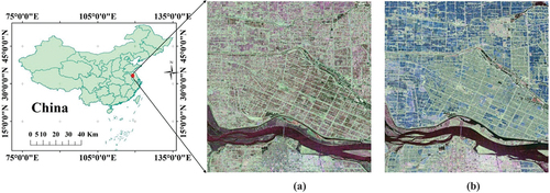
The study area consists of three regions. The first study area, shown in Figure 1, is the area near Jinhu, Huai‘an, Jiangsu, China, which is located at the junction of Jinhu, Hongze, and Xuyi with the central geographic coordinates of 33°07’05 “N and 118°59’ 55.14” E. The main crop in this area is rice. Due to the different rice variety selections and planting methods by farmland operators, this area is divided into two types of paddies: direct-sown japonica rice paddy (D-J) and transplanting hybrid rice paddy (T-H). The T-H rice is indica; the growth cycle is approximately 120 days with the transplanting planting mode. The D-J rice is japonica, and the growth cycle is approximately 150 days with the direct-sown planting method. Compared with transplanting paddy rice, rice in direct-sown paddies will show a random uniform distribution in the seedling stage, with no obvious regularity. Water, urban, and shoal areas are also included in the study area in addition to D-J and T-H. Therefore, we divided the study area into five classes.

Figure 1. The color composite images (FP SAR VV (red), VH (green), and HH (blue)) of the backscattering coefficients of FP SAR data (a: July 27, 2012; b: September 16, 2015).

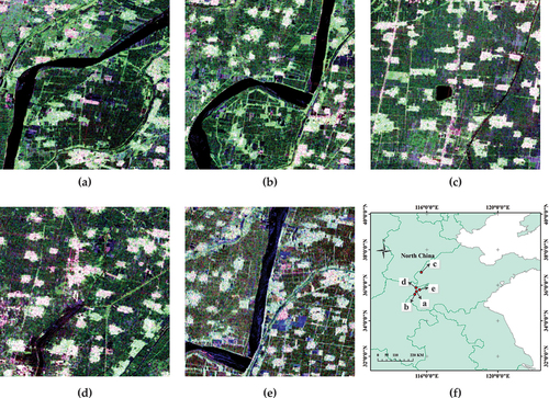
To prove the robustness of the transfer learning method in the fine classification of crops, we chose study area 2 (Yellow River basin in the North China Plain). The area contains three major ground objects (water, urban, and wheat). The wheat type cultivated in the North China Plain is winter wheat, which has a whole growing period of 190–210 days. It is generally sown in mid-late October of the Gregorian calendar and harvested in June of the following year. Because the study area is too large, we selected five small regions in the study area. Figure 2 shows the Pauli decomposition pseudo-color image of the study area.

Figure 2. The color composite images of Pauli decomposition of FP SAR data (a, b, c, and d are SAR images of regions a, b, c, and d of study area 2 on March 6, 2017, respectively. e is SAR images of small region e on May 22, 2017. f is the distribution map of the five small regions in study area 2).

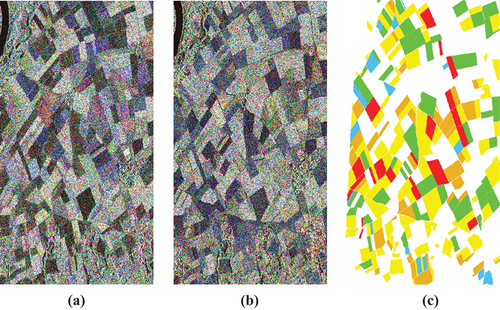
Additionally, we also chose study area 3 (Wallerfing, Germany) as our third study area with central geographic coordinates of 48°42′N, 12°54′E. The area contains barley, corn, potato, sugar beet, and wheat as five land types and is an ideal study area for the fine classification of crops. In this study area, from May to June, the phenology stage of wheat and barley planted is growth stage, and from July to August, the phenology stage of the two crops is the harvest stage. In addition, the sugar beet phenology stage in May is the seedling stage. In June, the phenology stage is growth stage, and in July and August, the sugar beet is gradually mature. For corn and potato, the growth stage is in May, and from June to August, the stalk of corn and potato no longer grow, and their fruits gradually mature. Figure 3 shows the Pauli decomposition pseudo-color image of the study area.

Figure 3. The color composite images of Pauli decomposition of FP SAR data (a: May 28, 2014; b: August 18, 2014; c: ground-truth data (blue, brown, red, green, and yellow plots are barley, corn, potato, sugar beet, and wheat, respectively).

2.2. Data collection

Due to the lack of real CP data, the CP SAR data in this study is obtained by simulation based on FP SAR data. For study area 1, we acquired a total of five temporal RADARSAT-2 full-polarization (Fine-Quad) single-look complex (SLC) data with a center frequency of 5.4 GHz (C band). Table 1 shows the detailed parameters of the multitemporal RADARSAT-2 C band data. The dataset contains data for two periods, 2012 and 2015. The phenological periods of rice covered by the 2012 and 2015 data are the seedling stage, seedling-elongation, booting-heading, heading-flowering, dough-mature, and mature stages, respectively. The purpose of selecting these 12 temporal data in study area 1 is to study the classification effect of the transfer learning method under the same phenological periods of rice across years and the different phenological periods across years, respectively. In addition, in study area 1, we selected 35 rice sample parcels (24 T-H plots and 11 D-J plots) and 8 water, 8 shoal, and 10 urban plots. When the RADARSAT-2 satellite transits, field surveyors use the high-precision Global Positioning System (GPS) to obtain the boundaries of these five kinds of ground objects as ground-truth data. A total of 56,266 samples were collected in study area 1. For supervised classification experiments, 60% and 40% of the samples were randomly split into training and validation sets, respectively. For the transfer experiments, 40% of the labeled samples were unchanged as the validation sets of the target domain, and the source and target domain labeled samples were randomly selected from the remaining 60% samples.

Table 1. Full-polarization SAR data parameters of multitemporal RADARSAT-2 C band data for study area 1.

Data acquisition (D/M/Y)	DoY (Day of Year)	Image mode	Pixel spacing (A × R, m)	Incidence angle (°)	Rice phenology stage
27/06/2012	179	FQ20W^1	5.2×7.6	38–41	Seedling
21/07/2012	203	FQ20W	5.2×7.6	38–41	Seedling-Elongation
28/08/2012	241	FQ9W	5.2×7.6	27–30	Booting-Heading
21/09/2012	265	FQ9W	5.2×7.6	27–30	Heading-Flowering
15/10/2012	289	FQ9W	5.2×7.6	27–30	Dough-Mature
08/11/2012	312	FQ9W	5.2×7.6	27–30	Harvest
12/06/2015	163	FQ20W	5.2×7.6	38–41	Seedling
30/07/2015	211	FQ20W	5.2×7.6	38–41	Seedling-Elongation
23/08/2015	235	FQ20W	5.2×7.6	38–41	Booting-Heading
16/09/2015	259	FQ20W	5.2×7.6	38–41	Heading-Flowering
10/10/2015	283	FQ20W	5.2×7.6	38–41	Dough-Mature
03/11/2015	307	FQ20W	5.2×7.6	38–41	Harvest

^aFQW = fine-quad-polarimetry wide, where 20 or 9 is the number of beam positions, which is related to the incidence angle.

For study area 2, we acquired five GF-3 full-polarization SLC data with a center frequency of 5.4 GHz (C band) from five small study area regions. The data receiving station is Miyun (KYN) receiving station. Image mode of GF-3 full-polarization SAR data is Quad Polarimetry Stripe. Table 2 shows the detailed parameter information of the multitemporal GF-3 C band data for study area 2. Specifically, the phenological period of wheat in the study area on March 6 is a regreening-elongation stage, which has obvious characteristics compared with other ground features and is conducive to ground feature classification. The wheat phenological period on May 22 is the mature stage and about to be harvested. Different from other objects, the distinct scattering characteristics are also conducive to classification. For study area 3, we acquired a total of four temporal RADARSAT-2 full-polarization SLC C band data. Table 3 shows the detailed parameter information.

Table 2. Full-polarization SAR data parameters of multitemporal GF-3 C band data for study area 2.

Small regions	Data acquisition (D/M/Y)	Image mode	Pixel spacing (A×R, m)	Incidence angle (°)	Wheat phenology stage
Small region a	06/03/2017 06/03/2017 06/03/2017 06/03/2017	QPSI^2	5.0×4.5	48.79	Regreening- elongation
Small region b		QPSI	5.0×4.5	48.79	Regreening- elongation
Small region c		QPSI	5.0×4.5	48.79	Regreening- elongation
Small region d		QPSI	5.0×4.5	48.79	Regreening- elongation
Small region e	22/05/2017	QPSI	2.2×5.2	34.63	Mature

^aQPS = Quad Polarimetry Stripe.

Table 3. Full-polarization SAR data parameters of multitemporal RADARSAT-2 C band data for study area 3.

Data acquisition (D/M/Y)	DoY (Day of Year)	Image mode	Pixel spacing (A×R, m)	Incidence angle (°)	Phenology stage
28/05/2014	148	FQ20W	5.2×7.7	40.2	Seedling stage
21/06/2014	172	FQ20W	5.2×7.7	40.2	Early growth stage
15/07/2014	196	FQ20W	5.2×7.7	40.2	Late growth stage
18/08/2014	229	FQ20W	5.2×7.7	40.2	Mature stage

The main preprocessing for the original FP SAR data in the study areas includes radiometric calibration and speckle filtering. First, the original FP data header file provides the parameters needed for the radiometric calibration phase. The image is then speckle filtered using a Lee filter. In general, different window filters are used to filter images of different resolutions. Too large filtering window leads to serious detail loss, while too small window leaves too much noise, and this noise can also be mistaken for details. The subsequent classification accuracy can be greatly influenced by the size of the window, whether it is too large or too small. On the one hand, the Pixel spacing (A × R, m) of the multi-temporal RADARSAT-2 C band data used in this study is 5.2 × 7.6 or 5.0 × 4.5. On the other hand, we try the Lee filter of 3 × 3, 5 × 5, 7 × 7, and 9 × 9 sizes to filter the image, respectively. By comparing the filtering effect, we find that the filtering effect of 7 × 7 Lee filter is the best, that is, it retains the details of objects and effectively removes a lot of noise. Therefore, both the resolution size of the data utilized and the filtering effect are duly considered. Ultimately, a 7 × 7 Lee filter is employed in this study to effectively enhance image quality (Guo et al. 2022; Rubel et al. 2021). For all GF3 and RADARSAT-2 FP SAR data, we extract the corresponding complex scattering matrix S of FP SAR data based on PolSARpro software (version 6.0, https://step.esa.int/main/toolboxes/polsarpro-v6–0-biomass-edition-toolbox/). Next, the preprocessing work is carried out in PolSARpro v6.0 and ENVI image processing software (version 5.3, https://www.nv5geospatialsoftware.com/Products/ENVI). In addition, the proposed algorithm and comparison algorithms in this study are programmed in matlab software (version R2021b, https://ww2.mathworks.cn/en/products/matlab.html) and python software (version 3.8, https://www.python.org/).

3. Methodology

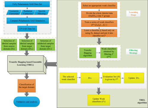
In this study, data preprocessing, including radiometric and geometric correction, filtering, and simulation of the CP SAR data, is first carried out based on the FP SAR data. Then, the proposed TBEL method is used to perform classification, in which the labeled samples of the source domain are denoted as D_S, and the labeled and unlabeled samples of the target domain are denoted as D_TL and D_TU, respectively. Finally, the classification results are analyzed. Figure 4 shows the methodology flowchart.

Figure 4. Methodology flowchart.

3.1. CP SAR data preparation

3.1.1. CP SAR data simulation

First, the CP SAR data are generated by simulation under different transmitting electromagnetic wave modes. At present, the most widely used CP modes are the π/4 mode (Souyris et al. 2005) and the CTLR mode (Raney 2007). In study areas 1 and 2, the CTLR mode is selected. The CTLR mode transmits circular polarization, receives horizontal and vertical polarization echo signals, and preserves some roll-invariant target properties.

On the single-pixel SLC level in the CP SAR system, the complex scattering matrix S projection is measured, as shown in (1) (Cloude, Goodenough, and Chen 2021),

(1) $\left[\begin{array}{c}{E}_{\mathit{HC}}\\ E_{\mathit{VC}}\end{array}\right]=\left[\begin{array}{cc}{S}_{\mathit{HH}}& S_{\mathit{HV}}\\ S_{\mathit{VH}}& S_{\mathit{VV}}\end{array}\right]E_i$(1)

where $\left[\begin{array}{c}{E}_{\mathit{HC}}\\ E_{\mathit{VC}}\end{array}\right]$ is the scattering vector ($\stackrel{\rightharpoonup }{\mathrm{k}}$) of the CP mode and E_i is the unit Jones vector of the radar transmit wave. For CTLR mode, $E_i=\frac{1}{\sqrt{2}}\left[\begin{array}{c}1\\ \pm \mathit{j}\end{array}\right]$, + indicates the left circular (LHC) transmit wave, and − indicates the right-hand circular (RHC) transmit wave.

Therefore, the${\stackrel{\rightharpoonup }{\mathrm{k}}}_{\mathrm{CTLR}}$ scattering vector under CTLR mode can be expressed as follows:

(2) ${\overrightarrow{\mathrm{k}}}_{\mathrm{CTLR}}=\frac{1}{\sqrt{2}}{\left[{\mathrm{S}}_{\mathrm{HH}}\pm \mathrm{j}{\mathrm{S}}_{\mathrm{HV}}{\mathrm{S}}_{\mathrm{HV}}\pm \mathrm{j}{\mathrm{S}}_{\mathrm{VV}}\right]}^{\mathit{T}}$(2)

The coherency matrix (C₂) of CP SAR is the second-order statistic of the scattering vector, which can be expressed as follows:

(3) $C_2=⟨{\overrightarrow{\mathrm{k}}}_{\mathit{CP}}{\overrightarrow{\mathrm{k}}}_{\mathit{CP}}^{\ast \mathit{T}}⟩$(3)

The Stokes matrix $\mathit{s}=\left[\begin{array}{cc}\begin{array}{cc}{g}_0& g_1\end{array}& \begin{array}{cc}{g}_2& g_3\end{array}\end{array}\right]$ is usually used to characterize the intensity and polarization of the scattering echoes, where the element represents the actual power measured value. Therefore, C₂ of CP SAR can be expressed by the Stokes matrix as follows:

(4) $C_2=\left[\begin{array}{cc}{C}_{11}& C_{12}\\ C_{12}^{\ast }& C_{22}\end{array}\right]=\frac{1}{2}\left[\begin{array}{cc}{g}_0+g_1& g_2-\mathit{i}{g}_3\\ g_2+\mathit{i}{g}_3& g_0-g_1\end{array}\right]$(4)

Then, the Stokes matrix can be expressed as follows:

(5) $S_{\mathit{CP}}=\left[\begin{array}{c}{g}_0\\ g_1\\ g_2\\ g_3\end{array}\right]=\left[\begin{array}{c}⟨C_{11}⟩+⟨C_{22}⟩\\ ⟨C_{11}⟩-⟨C_{22}⟩\\ 2Re(⟨C_{12}⟩)\\ -2Im(⟨C_{12}⟩)\end{array}\right]$(5)

It is possible to generate various parameters characterizing the received scattered wave from the Stokes vector. Four relevant quantitative sigma-naught backscatter parameters for circular transmit waves are given as follows.

The sigma-naught backscatter value at RH, RV, RR, and RL polarizations (Dabboor and Geldsetzer 2014; Dabboor and Shokr 2020; Yang et al. 2014):

(6) $\left\{\begin{array}{ccccc}{\sigma }_{\mathit{RH}}=& [1& 1& 0& 0]\mathit{s}\\ {\sigma }_{\mathit{RV}}=& [1& -1& 0& 0]\mathit{s}\\ {\sigma }_{\mathit{RR}}=& [1& 0& 0& -1]\mathit{s}\\ {\sigma }_{\mathit{RL}}=& [1& 0& 0& 1]\mathit{s}\end{array}\right.$(6)

Therefore, for each FP SAR dataset, we extracted eight CP parameters, including four Stokes parameters (g₀, g₁, g₂, g₃) and four backscattering coefficients (σ_RH, σ_RV, σ_RR, σ_RL), based on the simulation method CTLR mode. To study the effects of CP SAR data of different modes on the transfer learning-based method fine classification of various crops, we selected CTLR and π/4 modes in study area 3.

3.1.2. Selection datasets of D_S, D_TL, and D_TU

The source domain usually contains a substantial number of labeled training samples. In this study, we selected approximately 1,000–5,000 pixels from the source domain samples for each class. The target domain is the classification task dataset. Here, the target domain contains a small number of labeled samples. For each class in the target domain, we select approximately 100 pixels. In addition, D_TU is randomly selected in the unlabeled sample of the target domain with approximately 1,000–5,000 pixels. To study the effectiveness of the transfer learning method and explore the effect of the cross-year source domain on the target domain and the effect of the cross-phenological period source domain on the target domain, we conducted several different transfer experiments in three study areas.

Table 4 shows the transfer experiments of study area 1. For the source domain, we selected the simulated CP data of the CTLR mode on June 27, July 21, August 28, September 21, October 15, and 8 November 2012. For the target domain, we selected the simulated CP data of the CTLR mode on June 12 July 30, August 23, September 16, October 10, and 3 November 2015. Therefore, there is a one-to-one correspondence between the six phenological periods of 2012 and 2015 in the transfer experiment. Table 5 shows the transfer experiments of study area 2. We perform four transfer experiments. The source domain of the four transfer experiments is the simulated CP data of the CTLR mode in small region a on 6 March 2017. The target domain is the simulated CP data of the CTLR mode in small region b, small region c, and small region d on March 6, and small region e on May 22, respectively. Table 6 shows the transfer experiments of study area 3. A total of four FP SAR data, which, respectively, cover the seedling stage, growth stage, and mature stage of crop growth, were obtained in the study area.

Table 4. Transfer experiments in study area 1.

Transfer types	Experiments	Date of DS data	Date of DT data
Cross-year transfer under the same phenological periods	(a)	27/06/2012	12/06/2015
	(b)	21/07/2012	30/07/2015
	(c)	28/08/2012	23/08/2015
	(d)	21/09/2012	16/09/2015
	(e)	15/10/2012	10/10/2015
	(f)	08/11/2012	03/11/2015
Cross-year transfer under the different phenological periods	(g)	27/06/2012	10/10/2015
	(h)	21/09/2012	10/10/2015
	(i)	21/09/2012	03/11/2015

Table 5. Transfer experiments in study area 2.

Transfer types	Experiments	Region of DS data	Region of DT data
Transfer under the same phenological periods of similar scenes	(a)	Small region a	Small region b
	(b)	Small region a	Small region c
	(c)	Small region a	Small region d
Transfer under the different phenological periods of similar scenes	(d)	Small region a	Small region e

Table 6. Transfer experiments in study area 3.

Experiments	Date of DS data	Date of DT data
(a)	28/05/2014	21/06/2014
(b)	28/05/2014	15/07/2014
(c)	28/05/2014	18/08/2014
(d)	18/08/2014	28/05/2014
(e)	18/08/2014	21/06/2014
(f)	18/08/2014	15/07/2014

3.2. Transfer learning method

In the Transfer Bagging (TrBagg) (Kamishima, Hamasaki, and Akaho 2009) method, which is an inductive transfer method, the source domain data is regarded as data characterizing the concepts in the target domain and data not relating to the concepts in the target domain. Therefore, data from these two domains satisfy the complementary relationship: the labeled samples from the target domain are scarce, but they are closely related to the target domain task; although not all labeled samples from the source domain are reliable, they are rich in diversity. If the two domains can be combined, the key information highly related to the target domain task from the target domain data can be extracted, and source domain data can be used to enrich the information diversity of target tasks. Thus, the constructed classification model has the potential to better identify the category of the target domain. Bagging-based Ensemble Transfer Learning (BETL) method (Liu et al. 2016) constructs an evaluation set by combining the source and target domain data to train the classifier, evaluates the unlabeled samples from the target domain, and then uses these pseudo-labeled target domain samples to train the weak classifier. The method makes full use of the unlabeled target domain data.

It is not difficult to find that both methods have advantages and disadvantages. Although the TrBagg method reduces the negative transfer risk, it does not fully use the unlabeled samples in the target domain, which may lead to a low transfer effect. BETL extracts data subsets from only the source domain to establish a set of evaluation classifiers to assist in judging the unlabeled sample categories in the target domain. However, once the interdomain difference is too large or the sparse label samples from the target domain are not representative of the category, many misjudged pseudo-labeled samples from the target domain will be introduced for training, resulting in a strong negative transfer effect.

Because the source domain data contain both samples related to the target domain task and irrelevant samples, directly sampling from the source domain data to establish the evaluation classifier can introduce a large deviation. By prefiltering, improving the use effect of the evaluation set is possible. Therefore, inspired by TrBagg and BETL, a new method is proposed.

3.2.1. Transfer bagging (TrBagg) algorithm

The idea of the TrBagg algorithm is that a weak classifier learns from a total sample set, including a training sample subset of the source domain, the learned weak classifier classifies the target data, and the accuracy of the classification result is obtained for the target data. If the accuracy meets the condition, most of the samples used to train the weak classifier are considered consistent with the target domain samples. However, the classifier is abandoned if the classification accuracy does not meet the condition. Weak classifiers consistent with the target domain can be obtained by iterating these processes. In this way, the weak classifier is obtained, and the majority voting on the classification results of weak classifiers determines the final classes. The TrBagg algorithm can be divided into two stages: the learning stage and the filtering stage.

1. Learning stage: The labeled sample set is first combined, which consists of labeled samples in the source domain and the target domain, namely, D_SUD_TL. Then, according to the combined labeled sample set, random sampling with retractions is performed to obtain T training subsets, and based on these training subsets, T weak classifiers (F={f₁,f₂,f₃ … f_T}) are trained.

2. Filtering stage: This stage refines the weak classifier set F obtained from the learning stage to select the weak classifier set F* that is effective for the target task. The evaluation is based on assessing the performance of a series of weak classifiers in the target domain using a limited number of labeled samples (D_TL). If the classification accuracy is high, which indicates that most of the samples in the corresponding training sample subset are related to the target domain information, the classifier is selected into F *. Otherwise, the classifier will be filtered out if the training sample subset is not associated with the target domain.

Additionally, the TrBagg algorithm encompasses two pivotal aspects. First, in the filtering stage, a series of weak classifiers predict the classes of the target domain through the majority of the judgment results. The bagging prediction function (Kamishima, Hamasaki, and Akaho 2009) can be expressed as:

(7) $\mathit{C}=arg\underset{\mathit{c}\in \mathit{C}}{max}\sum _{\mathit{i}=1}^T\mathrm{I}[\mathit{c}=f_i(\mathit{x})]$(7)

where I[.] is a binary function whose value is 1 if the value in square brackets is true and 0 otherwise. C represents the set of class labels.

Second, before filtering, a classifier trained entirely on the target domain labeled sample set is introduced to avoid negative transfer effects that can result when utilizing source domain data. This classifier is called the fallback classifier. Even in the worst case, where the source domain data is completely useless to the target domain task, the fallback classifier ensures that there will be no degradation in target domain task accuracy.

3.2.2. TBEL algorithm

The two core tasks of the TBEL algorithm are to make full use of source domain information, that is, to select valuable source domain labeled samples and to formulate an excellent evaluation set to select useful target domain unlabeled samples to improve crop classification accuracy.

The target domains contain unlabeled samples related to the target domain task and some unrelated samples. Based on the TBEL algorithm, first, unlabeled samples (D_TU) are established. Here, D_TU is randomly selected in the target domain and contains samples of all kinds of ground objects in the target domain. This algorithm then considers a set of judgments H and evaluates the unlabeled samples (D_TU) in the target domain. Thus, unlabeled samples that are useful to the target domain are selected. Next, the D_TU of the pseudo-notation that is useful for the target task is used to train the weak classifier for transfer learning-based method classification. Considering the importance of judging set H, if we select a good H, which is a classifier set trained from sample data related to the target domain, it will improve the judging set H and thus improve the final classification accuracy. However, BETL trains the classifier by combining the D_S and D_TL data to form a judgment set H and evaluates the unlabeled samples (D_TU) in the target domain. Since the source domain contains some samples related to the target domain task and some unrelated samples, the judging set H in the BETL algorithm is a classifier set trained by a sample subset containing both source and target domain labeled samples, which introduces large errors to the judging set H. However, the TrBagg algorithm makes full use of the sample information of the source domain. It avoids negative transfer by filtering the samples unrelated to the target task and introducing a fallback classifier. If we use the weak classifier set trained by the filtered samples as the judgment set H, the ability to optimize the selection of unlabeled samples will significantly improve and, thus, improve the final classification accuracy. Therefore, we proposed the TBEL algorithm. The specific idea of the TBEL algorithm is to use the filtered classifier set trained as the evaluation set and to interpret unlabeled samples in the target domain based on the evaluation set. The details include two steps.

Step 1: initialization stage. Using the TrBagg algorithm in Section 3.2.1, the D_S and D_TL datasets are used to obtain F* after filtering, and F* after filtering is used as the judging set H. In addition, the D_TU in target tasks needs to be prepared.

Step 2: update stage. First, each classifier in judging set H is used to predict the D_TU classes, the data with consistent prediction results are added to the labeled target domain set (D_TL), and the first weak classifier is trained based on the new set. Then, the unlabeled sample classes are predicted using the judging set H classifier and the updated weak classifier in the previous calculation, and the data with consistent prediction are added to the original labeled sample set in the D_TL. Next, the weak classifier is trained based on this new set in this calculation. The iteration is stopped when the target domain data does not change again, or the number of iterations reaches the upper limit (N). Therefore, N weak classifiers with successive updates can be obtained after N iterations, and the prediction classes of unknown samples can be obtained by voting with these N weak classifiers. The detailed steps of the TBEL algorithm are shown in the proposed algorithm.

Table

The proposed TBEL algorithm
1 Select an appropriate weak classifier, preparing DS,DTL, and DTU.
2 The training samplesubset is generated by dividing the whole labeled data (DSUDTL)into Tgroups.
3 Implement the TrBagg algorithm.
4 Obtain F* by filtering F, and F*is used as the judging set H.
5 For n =1,2,3…Ndo
6 Classify DTUby using classifiers in the judging set H.
7 If n =1then
8 Add the data that is completely consistent with the DTUprediction classes to DTL.
9 else
10 Compare the prediction ofH to DTUwith the prediction of ft-1 to DTU, and add the data that is completely consistent with DTL.
11 end if
12 Use DTL to train a weak classifier ft and add the weak classifier to weak classifier set F.
13 If DTL no longer changes then
14 break
15 end if
16 end for
17 Obtain weak classifier set FT.

4. Results and discussion

4.1. Cross-year rice classification based on transfer learning method

We conducted the experiments of cross-year rice classification in study area 1. First, we selected three weak classifiers (decision tree, random forest, and K-nearest neighbor classifiers) to accurately classify two types of rice using CP SAR data of the CTLR mode based on the TBEL algorithm, respectively. Based on this algorithm, transfer experiments for the fine classification of rice in nine groups were carried out. To better evaluate the performance of the TBEL algorithm, we added an algorithm comparison experiment and introduced inductive and transductive transfer learning methods proposed by some researchers. TrBagg and BETL are used for experimental comparison of the inductive transfer learning methods, and the maps of the experimental results and precision table are given. In addition, for the transductive transfer learning methods, we used geometric feature-based transfer learning methods, including Subspace Alignment (SA) (Fernando et al. 2014), CORrelation ALignment (CORAL) (Sun, Feng, and Saenko 2016), and statistical feature-based transfer learning methods, including Joint Distribution Adaptation (JDA) (Long et al. 2013), and Balanced Distribution Adaptation (BDA) (Wang et al. 2017).

Figure 5 shows the fine classification of two types of rice based on three transfer learning algorithms (TrBagg, and TBEL algorithms) under six group transfer experiments using random forest as a weak classifier. a, b, c, d, e, f, g, h, and i represent the transfer experiments in six groups of cross-year domains under the same phenological periods and three groups of cross-year domains under different phenological periods.

Figure 5. Fine classification maps of two types of rice based on three transfer learning algorithms (TrBagg, BETL, and TBEL) in six groups of transfer experiments (a, b, c, d, e, and f are the transfer experiments in six groups of cross-year domains under the same phenological periods, and serial 1, 2, and 3 are the fine classifications of rice results based on the TrBagg, BETL, and TBEL algorithms, respectively). gt is the ground-truth area of five kinds of ground objects).

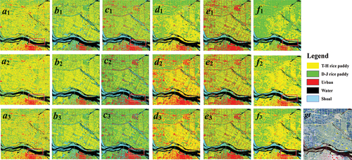
As shown in Figure 5, T-H is located in the southeastern part of the study area, D-J is located in the northwestern part of the study area, city buildings of the urban class are located in the southern part of the study area, and small towns of the urban class are distributed throughout the study area. The classification results are consistent with the actual situation. a, b, c, d, e, and f are cross-year transfer experiments under the same seedling stages, seedling-elongation, booting-heading, heading-flowering, dough-mature, and harvest stages, respectively. According to the classification results, the better performance of T-H and D-J distinction is presented with rice growth, especially in the heading-flowering and harvest stages. Taking the transfer experiment of the same harvest stages in the cross-year domain as an example, T-H was harvested during this period; D-J was still in the mature stage. Therefore, on the radar image, the scattering characteristics of the two types of rice are obviously different. In the transfer, the difference between the two types of rice in the source domain is obviously promoted in the target domain, and the transfer learning-based method classification result of the same harvest stage in the cross-year domain is better.

Comparing the classification results of the three transfer learning algorithms (serial 1, 2, 3), the overall classification maps are not very different, but the details are somewhat different. The regions located at the red rectangle in Figure 5a₁, a₂, a₃, Figure 5c₁, c₂, c₃, and Figure 5f₁, f₂, f₃ are quite different. For example, in Figure 5c₁, c₂, c₃, the ground-truth class of the red rectangle is water. The classification results in Figure 5c₁ and 5c₂ are partially misclassified into the shoal class; however, in Figure 5c_3, the classification result is most consistent with the actual water class. Therefore, in detail, the classification results based on the TBEL algorithm are better than those based on the TrBagg and BETL algorithms. In addition, Figure 6 shows the fine classification of two types of rice based on three algorithms under three groups of transfer experiments using random forest as a weak classifier. Figure 6g, h, and i are cross-year transfer experiments of different phenological periods. The classification results are basically the same. For example, for Figure 6g₁, g₂, and g₃, the ground-truth class in the red rectangle is water, and Figure 6g₃ is most consistent with the actual water class. However, there are partial misclassifications in Figure 6g₁ and g₂.

Figure 6. Fine classification maps of two types of rice based on three transfer learning algorithms (TrBagg, BETL, and TBEL) in three transfer experiments (g, h, and i are three groups of cross-year domains under different phenological periods).

To better evaluate the classification results, Table 7 shows the transfer learning-based classification accuracy with weak decision tree classifiers. As shown in the classification accuracy table, the classification results based on the TrBagg, BETL, and TBEL algorithms are better than those based on geometric and statistical feature-based transfer learning methods. This is because the transductive transfer learning methods do not require labeled samples in the target domain (Fernando et al. 2014; Qin et al. 2020). This also demonstrates the importance of labeled samples of the target domain. For TrBagg algorithm, the result accuracy is not too low, because the fallback classifier is built, which can avoid the negative transfer (Kamishima, Hamasaki, and Akaho 2009). In addition, comparing the TrBagg, BETL, and TBEL algorithms, the classification result based on the TBEL algorithm is better than that of the TrBagg and BETL algorithms. The overall accuracy of the TBEL algorithm is 0–6% higher or close to the accuracy of the supervision classification results. The main reason is that the TBEL algorithm proposed in this study not only avoids the negative transfer of the target task but also uses the unlabeled sample information in the target domain by selecting representative training samples. In addition, its judging set H helps to select useful pseudo-label samples in the target domain (Liu et al. 2016).

Table 7. Transfer learning-based method classification overall accuracy (OA) table with a decision tree as a weak classifier.

Transfer learning algorithms	Transfer experiments (OA/%)
	a	b	c	d	e	f	g	h	i
SA (Fernando et al. 2014)	32.5	26.5	41.8	40.5	41.7	59.8	14.2	57.8	33.9
CORAL (Sun, Feng, and Saenko 2016)	33.2	57.6	54.8	48.2	48.9	52.7	41.7	43.5	42.2
JDA (Long et al. 2013)	41.2	44.5	64.7	67.7	38.4	46.9	39.9	69.0	47.6
BDA (Wang et al. 2017)	33.5	54.1	46.9	26.0	32.6	33.6	57.2	29.3	42.1
TrBagg (Kamishima, Hamasaki, and Akaho 2009)	62.4	75.4	71.5	81.3	75.2	88.2	73.7	77.2	81.1
BETL (X. Liu et al. 2016)	62.8	74.1	75.6	84.8	79.7	87.8	73.9	78.9	89.6
TBEL	67.3	76.3	71.6	86.5	81.0	92.2	79.6	78.2	92.7
Supervised classification	67.0	79.6	75.5	85.8	89.5	94.0	89.5	89.5	94.0

By comparing transfer experiments (a, b, c, d, e, and f) based on the TBEL algorithm, the transfer learning-based classification (f) of the same harvest stage in the cross-year domain has the highest accuracy, with an overall accuracy of 92.2%, followed by the transfer learning-based classification (d) with the same heading-flowering stage in the cross-year domain, with an overall accuracy of 86.5%. The main reason is that in the two phenological periods, the difference between the two types of rice on the radar image is obvious, which contributes to the transfer of rice characteristics. Furthermore, for rice cross-years transfer under the same phenological periods, the classification accuracy of the six transfer cases from cross-years transfer under the same seedling stage to that under the same harvest stages shows an increasing trend. By comparing transfer experiments (g, h, and i), the transfer learning-based method classification of different phenological periods in cross-year domains shows that the classification result (i) of the phenological period in the source domain with the heading-flowering stage and target domain with the harvest stage has the highest accuracy of approximately 93.5%. That is, when rice is mature or at the harvest stage, the differences between T-H and D-J are conducive to feature transfer. Compared with Figure 5e and Figure 6g, the rice phenological period in the source domain is the dough-mature and heading-flowering stages, and the rice phenological period in the target domain is the dough-mature stage. The classification accuracy of transfer experiment e is better than that of g, indicating that the transfer learning-based method classification results of the same phenological periods are better than those of different phenological periods in cross-year domains.

To study the influence of different weak classifiers on the results of transfer learning-based method classification, we use the K-nearest neighbor classifier and random forest classifier to carry out transfer learning-based method classification experiments in addition to using the decision tree classifier. Table 8 shows the transfer learning-based method classification accuracy with K-nearest neighbor as a weak classifier. Table 9 shows the transfer learning-based method classification accuracy with random forest as a weak classifier. Similar to Table 7, the classification results of Table 8 and Table 9 based on TrBagg, BETL, and TBEL are better than those based on geometric and statistical feature-based transfer learning methods. Comparing transfer experiments (a, b, c, d, e, and f) based on the TBEL algorithm, the transfer learning-based method classification (f) of the same harvest stage in the cross-year domain has the highest accuracy, with overall accuracies of 93.9% and 95.9%.

Table 8. Transfer learning-based method classification OA table with K-nearest neighbor classifier as a weak classifier.

Transfer learning algorithms	Transfer experiments (OA/%)
	a	b	c	d	e	f	g	h	i
SA	58.8	66.8	61.6	62.6	28.1	65.7	26.5	56.9	61.6
CORAL	54.2	63.2	54.6	48.6	27.9	52.3	53.7	48.4	49.0
JDA	46.0	46.0	65.6	72.6	36.3	47.5	41.8	70.6	55.0
BDA	45.4	46.3	64.5	75.4	36.6	47.4	40.2	71.2	55.9
TrBagg	62.6	75.7	70.7	82.7	79.6	88.5	70.8	80.8	90.9
BETL	61.0	75.2	74.7	85.2	81.8	90.7	72.3	82.3	89.8
TBEL	63.4	75.9	72.0	86.0	82.6	93.9	81.5	82.4	93.5
Supervised classification	66.6	80.7	76.9	86.5	83.2	94.5	83.2	83.2	94.5

Table 9. Transfer learning-based method classification OA table with random forest as a weak classifier.

Transfer learning algorithms	Transfer experiments (OA/%)
	a	b	c	d	e	f	g	h	i
SA	34.7	33.8	37.1	55.1	49.7	72.8	31.6	57.8	59.2
CORAL	35.0	57.8	52.7	46.4	45.3	48.7	47.0	43.6	42.8
JDA	40.0	48.8	67.5	71.5	37.7	49.6	38.1	72.2	59.5
BDA	30.8	26.6	44.4	10.3	22.6	20.2	51.5	16.1	24.8
TrBagg	64.8	77.1	72.4	83.6	81.3	93.5	73.8	81.8	90.1
BETL	64.3	76.8	72.5	86.0	83.2	93.5	77.6	82.6	91.5
TBEL	65.9	78.0	76.6	86.5	84.5	95.9	82.1	85.2	93.4
Supervised classification	70.2	84.0	80.7	90.8	86.9	94.5	86.9	86.9	94.5

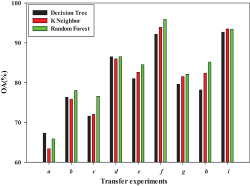
Figure 7 shows the classification accuracy based on the TBEL algorithm with different weak classifiers to better evaluate the performance of the three weak classifiers in the transfer experiment. As Figure 7 shows, random forest performs best among the nine transfer groups. Compared with transfer experiments a-f, the classification accuracy based on the TBEL algorithm presents an overall increasing trend, with transfer experiment f showing the best performance. That is, the difference between the two types of rice is obvious with rice growth, which is conducive to classifying the T-H and D-J characteristics. Comparing the transfer experiments (e, g, and h), the phenological periods of the source domain are the dough-mature, seedling, and heading-flowering stages, respectively, and both target domains are in the dough-mature stage. The highest accuracy of transfer learning-based method classification is e, followed by h, and the worst is g. Therefore, it can be concluded that the closer the rice phenological period is in the source and target domains, the better the transfer effect and the higher the classification accuracy.

Figure 7. The TBEL transfer learning-based method classification accuracy with different weak classifiers.

4.2. Cross- scenes wheat classification based on transfer learning method

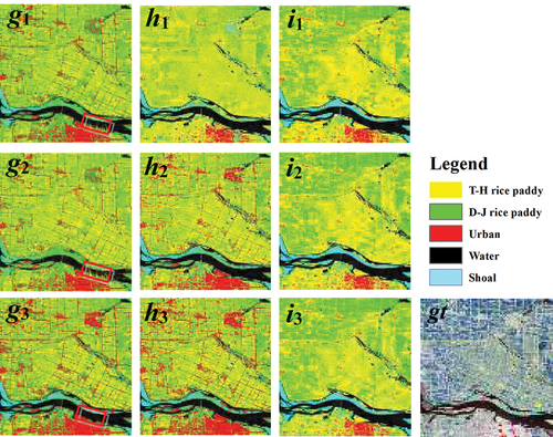
To verify the robustness and practicability of the TBEL algorithm, we also conducted transfer experiments of wheat classification in study area 2. Figure 8 shows the classification results of wheat based on the TrBagg, BETL, and TBEL algorithms under four groups of transfer experiments using random forest as a weak classifier. Figure 8a, b, and c represent the transfer experiments under the same phenological periods of similar scenes. Figure 8d represents the transfer experiment under different phenological periods of similar scenes.

Figure 8. Classification maps of wheat based on the TrBagg, BETL, and TBEL algorithms under four groups of transfer experiments (a, b, and c are transfer experiments under the same phenological periods of similar scenes. d is the transfer experiment under different phenological periods of similar scenes, and serial 1, 2, and 3 are the classification results based on the TrBagg, BETL, and TBEL algorithms, respectively).

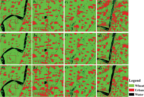
As shown in Figure 8a, the Yellow River runs through small region b, and the urban class is distributed throughout the image. The wheat class is distributed around the urban class. The classification results are consistent with the actual local situation. Comparing the transfer learning-based method classification results of the three algorithms, the classification results of Figure 8a₁ and Figure 8a₃ are similar. In contrast, in Figure 8a₂, there is a missing part for the urban class. For example, it is most obvious in the red rectangle of Figure 8a. For Figure 8b, the target domain is small region c, and the three algorithms separate the three ground objects, but the details are somewhat different. For example, the red rectangle region of Figure 8b is obvious. For Figure 8c, the ground truth in the red rectangle is the water class. Comparing Figure 8c₁, c₂, and c₃, the classification result of the TBEL algorithm (Figure 8c₃) shows that the water can be correctly identified. For Figure 8d, the Yellow River runs through small region e. The three algorithms distinguish the three types of ground objects. However, by comparing the three classification results, it can be clearly seen that for the classification results shown in Figure 8d₁ and Figure 8d₂, the wheat class is mixed with the water class, while in Figure 8d₃, there is no wheat class. The classification result of the TBEL algorithm is better than that of the TrBagg and BETL algorithms.

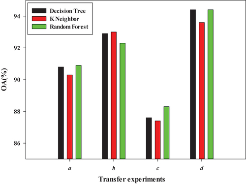
We quantitatively analyze the transfer learning-based method classification results to evaluate the performance of the transfer learning-based classification algorithm. Table 10–12 show the OA of the transfer learning-based method classification with decision tree, K-nearest neighbor classifier, and random forest as weak classifiers, respectively. Taking Table 10 as an example, for a group, the overall classification accuracy based on the TBEL algorithm can reach 90%, which is much higher than that of the SA, CORAL, JDA, and BDA transfer learning algorithms. The overall classification accuracy is 2–6% higher than that of the TrBagg and BETL algorithms. For group b, the overall classification accuracy based on the TBEL algorithm can reach 92%, which is 2–6% higher than that of the TrBagg and BETL algorithms. For the c group, the overall classification accuracy based on the TBEL algorithm can reach 87%, which is 3–10% higher than that of the TrBagg and BETL algorithms. For the d group, the transfer learning-based method classification results based on the TBEL algorithm can reach an OA of 94%, which is 6–8% higher than that of the TrBagg and BETL algorithms. Therefore, it can be seen in general that comparing the seven transfer learning algorithms, the transfer learning-based method wheat classification under the same phenological periods of similar scenes and the different phenological periods of similar scenes based on the TBEL algorithm can obtain better classification results with an overall classification accuracy of more than 87.6%, and the algorithms are more stable.

Table 10. Transfer learning-based method classification overall accuracy (OA) table with a decision tree as a weak classifier.

Transfer learning algorithms	Transfer experiments
	a		b		c		d
	OA (%)	Kappa	OA (%)	Kappa	OA (%)	Kappa	OA (%)	Kappa
SA	49.7	0.242	66.2	0.481	37.6	0.046	49.7	0.255
CORAL	66.3	0.498	67.0	0.500	86.4	0.795	73.1	0.590
JDA	65.7	0.480	80.8	0.707	81.6	0.723	83.5	0.753
BDA	56.1	0.336	77.0	0.648	59.6	0.382	58.4	0.386
TrBagg	88.4	0.807	92.1	0.877	84.0	0.739	86.6	0.799
BETL	84.6	0.745	89.8	0.842	77.2	0.630	88.1	0.821
TBEL	90.8	0.846	92.9	0.881	87.6	0.801	94.4	0.944
Supervised classification	91.9	0.863	94.0	0.905	88.8	0.821	93.5	0.901

Table 11. Transfer learning-based method classification OA table with K-nearest neighbor classifier as a weak classifier.

Transfer learning algorithms	Transfer experiments
	a		b		c		d
	OA (%)	Kappa	OA (%)	Kappa	OA (%)	Kappa	OA (%)	Kappa
SA	77.0	0.656	65.8	0.476	69.5	0.528	80.3	0.701
CORAL	71.4	0.573	60.3	0.391	84.8	0.772	76.6	0.645
JDA	65.5	0.478	80.4	0.700	81.7	0.725	80.4	0.708
BDA	64.7	0.465	80.2	0.698	81.3	0.719	79.5	0.694
TrBagg	89.3	0.821	92.4	0.881	83.8	0.736	89.2	0.838
BETL	85.1	0.754	90.5	0.853	81.7	0.705	89.1	0.836
TBEL	90.3	0.838	93.0	0.882	87.4	0.798	93.6	0.903
Supervised classification	89.5	0.825	94.3	0.910	86.5	0.786	93.8	0.905

Table 12. Transfer learning-based method classification OA table with random forest as a weak classifier.

Transfer learning algorithms	Transfer experiments
	a		b		c		d
	OA (%)	Kappa	OA (%)	Kappa	OA (%)	Kappa	OA (%)	Kappa
SA	76.5	0.649	66.4	0.484	54.4	0.299	62.6	0.447
CORAL	65.5	0.486	66.8	0.496	89.0	0.833	72.9	0.588
JDA	66.0	0.485	68.8	0.503	84.9	0.773	65.5	0.488
BDA	37.6	0.046	68.1	0.508	31.9	0.041	58.4	0.387
TrBagg	88.7	0.813	92.6	0.885	84.5	0.749	87.6	0.814
BETL	85.7	0.762	92.4	0.882	83.9	0.741	90.6	0.858
TBEL	90.9	0.847	92.3	0.872	88.3	0.812	94.4	0.915
Supervised classification	91.9	0.864	94.0	0.906	88.4	0.815	92.2	0.882

In addition, among the four groups, higher precision of classification results can be obtained based on inductive transfer learning methods than the four transductive transfer learning methods. By comparing the classification results of the three inductive transfer learning algorithms, the TBEL algorithm is the best, and its classification accuracy is close to that of the supervised classification results, which is 1–10% higher than that of the TrBagg and BETL algorithms, especially for transfer (d) under different phenological periods of similar scenes.

Similarly, to better evaluate the performance of three weak classifiers in the transfer experiment, Figure 9 shows the TBEL transfer learning-based method classification accuracy with different weak classifiers. As shown in Figure 9, comparing the three weak classifiers, there is little difference in the performance of the classification results in each group. Based on the TBEL method, the overall classification accuracy can be larger than 87%, and the highest OA can reach 94%. In addition, there are differences in the classification results for Figure 9a, b, and c. The main reason is that the quality of transfer learning-based method classification across similar scenes depends on the feature difference between the target and source domains. The greater the difference between the target and source domains, the more difficult it is to obtain better transfer learning-based method classification results. Among the four groups, the transfer experiment shown in Figure 9d has the best classification result, which can reach an overall classification accuracy of more than 93%. The TBEL algorithm proposed in this research can also obtain good transfer learning-based method classification results under different phenological periods of similar scenes.

Figure 9. The TBEL transfer learning-based method classification accuracy with different weak classifiers.

4.3. Fine classification of various crops based on transfer learning method

We conducted the experiments in an area with complex terrain types. To study the effects of CP SAR data of different modes on the transfer learning-based method fine classification of various crops, we selected random forest as the weak classifier to perform six transfer experiments using CP SAR data of CTLR and π/4 modes based on the TBEL algorithm. Figure 10 shows a crop classification map based on a random forest classifier using CP SAR of CTLR mode.

Figure 10. Fine classification maps of crops based on three transfer algorithms (TrBagg, BETL, and TBEL) using CP SAR of CTLR mode (a, b, c, d, e, and f are six transfer experiments, and a1-f1, a2-f2, and a3-f3 are the transfer classification results based on the TrBagg, BETL, and TBEL algorithms, respectively).

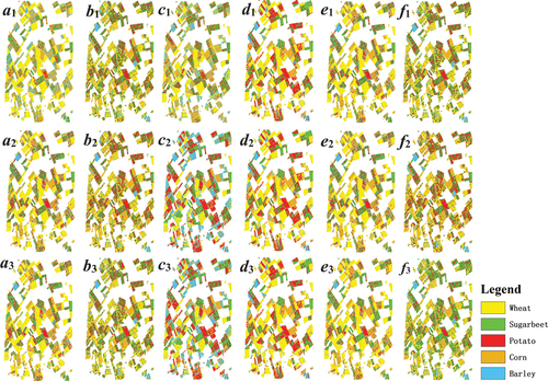
As Figure 10 shows, the five types of crops are classified, but the classification results in different periods are different. To better evaluate the classification results, Table 13 shows the classification accuracy of the transfer algorithms. It can be seen from the classification accuracy that the classification results of a, d, and e are good. The overall classification accuracy based on the TBEL algorithm can reach more than 60%. In other words, transfers from May 28 (seedling stage) to June 21 (early growth stage) and from August 18 (mature stage) to May 28 and June 21 are more effective. In addition, Table 13 shows that the classification results are poor when the source domain is transferred from May 28 and August 18 to July 15 (late growth stage). The main reason is that on July 15, the growth of all kinds of crops is completed, and the performance of all kinds of features has a high degree of similarity, which leads to the poor classification results of this phenological stage. Therefore, in the transfer process, its transfer ability is greatly reduced. Furthermore, for the transfer experiments of a, c and e, the overall classification accuracy based on the TBEL algorithm is 2%−6% higher than that based on the TrBagg and BETL algorithms. For transfer experiments b, d, and f, the overall classification accuracy based on the TBEL algorithm is 0%−2% higher than that of the TrBagg and BETL algorithms. Therefore, it is consistent with the experimental results in study areas 1 and 2. The TBEL algorithm is more stable than the TrBagg and BETL algorithms, and the obtained transfer classification accuracy is higher.

Table 13. Transfer classification accuracy based on three transfer algorithms.

Transfer Experiment	TrBagg		BELT		TBEL
	OA (%)	Kappa	OA (%)	Kappa	OA (%)	Kappa
a	54.7	0.404	59.9	0.471	61.5	0.490
b	42.3	0.253	40.9	0.242	42.5	0.253
c	49.9	0.364	49.4	0.381	51.4	0.399
d	64.2	0.528	62.8	0.512	64.3	0.528
e	60.1	0.474	59.9	0.473	62.1	0.494
f	42.2	0.251	41.5	0.252	42.6	0.257

Moreover, we also carried out six transfer experiments based on the TBEL algorithm of CP SAR data of the π/4 mode. Figure 11 shows the crop classification accuracy based on the TBEL algorithm using CP SAR of CTLR and π/4 modes. Figure 11 shows that the transfer classification accuracy of a, d, and e using CP SAR data of the two modes is high, which can achieve a classification accuracy of more than 60%. In addition, the classification accuracy using CP SAR data of the two modes is slightly different, approximately 2–3%. For transfer experiments a, b, c, e, and f, the transfer classification accuracy using CP SAR data in CTLR mode is higher than that using CP SAR data in π/4 mode. Only for transfer experiments of d, the classification accuracy using CP SAR data of π/4 mode is approximately 2–3% higher than that of using CP SAR data of CTLR mode. Therefore, the CP SAR data of different modes slightly differ in transfer classification, and the OA difference is approximately 2–3%. This variance of classification results is mainly due to the difference in the crop growth process, and the polarization signals of different transmitting and receiving modes are slightly different in showing that this variance of classification results in crop performance characteristics. In summary, for the fine classification of various crops based on the transfer learning, the CP SAR data of the CTLR mode perform better than the CP SAR data of the π/4 mode in most cases.

Figure 11. Transfer classification accuracy of crops based on the TBEL algorithm using CP SAR of CTLR and π/4 modes.

Based on our proposed algorithm, the time complexity of the trained classification model mainly includes two aspects. (1) The time complexity of obtaining the judgment set H, whose time complexity is O(T), where T is the number of training subsets of the source domain. (2) The time complexity of selecting the unlabeled samples in the target domain to train weak classifiers. The time complexity of this part is O(N), where N is the number of iterations for selecting the unlabeled samples in the target domain. Since each iteration needs to train the weak classifier once, the time consumption of this algorithm is mainly in the second aspect. Therefore, the computational efficiency of training weak classifiers affects the overall algorithm efficiency. However, in TBEL algorithm, weak classifier training requires a small number of pixels, which makes the training time of weak classifiers very short.

For different sizes of experimental scenarios, since the number of samples in the source and target domains is given a fixed range in the TBEL algorithm, the time consumption difference of training classifier model is not significant. However, scene size affects the computational efficiency of the model for the testing stage of experimental scenes. It should be noted that the main purpose of our proposed algorithm is to obtain a well-trained classification model. This model still belongs to the selected weak classifier type of the first step in the TBEL algorithm process. Therefore, the selection of different weak classifiers affects the computational efficiency for the testing stage of experimental scenes. In this study, we selected three kinds of weak classifiers, respectively, for classification experiments. Their computational efficiency (computation time: 21.96~144.96 s) in the transfer learning-based method classification experiment of large scene (pixel size: 2191 × 2295) is acceptable. In addition, the present parallel computing method can also improve the computational efficiency of the proposed method to a certain extent.

5. Conclusion

With the rapid development of SAR sensors, there has been a significant increase in the volume of collected data; however, acquiring labeled samples remains challenging. In the case of a small number of labeled samples, this study proposes the TBEL transfer learning method to ensure high accuracy in applying large-area fine classification of crops with CP SAR data. Specifically, we studied fine classification of two types of rice and wheat classification and fine classification of various crops based on TBEL transfer learning method. The specific conclusions are as follows:

1. For rice cross-years transfer, we find that the classification results of cross-years under the same phenological periods are better than those under different phenological periods. The transfer learning classification of the same harvest stage in the cross-year domain has the highest accuracy, with an OA of 92.2%, followed by the transfer learning-based method classification with the same heading-flowering stage in the cross-year domain, with an OA of 86.5%. Additionally, for rice cross-years transfer under the same phenological periods, classification accuracy of cross-years transfer under the same harvest stage is higher than that under the same seedling stage.

2. For wheat cross-scenes transfer, based on the TBEL algorithm, the overall accuracy can obtain better classification results, with an overall classification accuracy of more than 87.6%, especially under different phenological periods.

3. For fine classification of various crops based on transfer learning methods, the TBEL algorithm also achieves good fine classification of various crop results. Moreover, we find that the CP SAR data of the CTLR mode perform better than the CP SAR data of the π/4 mode in most cases. This conclusion agrees with single-scene applications and was first verified in transfer learning.

For crop classification with a small number of samples in the target domain, we use the weak classifier set trained by the filtered labeled samples as the judgment set. This idea improves the ability of unlabeled samples selection in the target domain, thus improving the final crop classification accuracy. This has been well demonstrated in rice, wheat, and various crop fields. However, for various crop classification tasks, the proposed algorithm has limited effect on improving classification accuracy. In the future research, in view of the difficulty of classifying multi-type crops and the low classification accuracy, we will fully consider the differences in the scattering characteristics of various crops, so as to further improve the classification accuracy of various crops.

Acknowledgments

The authors thank DLR (German Aerospace Center) for providing the Wallerfing data and making the ground truth data available.

Disclosure statement

No potential conflict of interest was reported by the author(s).

Data availability statement

The data that support the findings of this study are available upon reasonable request from the first author [Xianyu Guo. E-mall: http://[email protected]].

Supplementary material

Supplemental data for this article can be accessed online at https://doi.org/10.1080/15481603.2024.2319939

Additional information

Funding

This work was supported by NSFC under Grant no. 62222102, NSFC no. 62171023 and the. Fundamental Research Funds for the Central Universities under Grant no. FRF-TP-22-005C1.

References

- Charbonneau, F. J., B. Brisco, R. K. Raney, H. Mcnairn, C. Liu, P. W. Vachon, J. Shang, et al. 2010. “Compact Polarimetry Overview and Applications Assessment.” Canadian Journal of Remote Sensing 36 (2): S298–22. https://doi.org/10.5589/m10-062.
- Cloude, S. R., D. G. Goodenough, and H. Chen. 2021. “Compact Decomposition Theory.” IEEE Geoscience and Remote Sensing Letters 9 (1): 28. https://doi.org/10.1109/LGRS.2011.2158983.
- Collins, M., M. Denbina, and G. Atteia. 2013. “On the Reconstruction of Quad-Pol SAR Data from Compact Polarimetry Data for Ocean Target Detection.” IEEE Transactions on Geoscience and Remote Sensing 51 (1): 591–600. https://doi.org/10.1109/TGRS.2012.2199760.
- Dabboor, M., and T. Geldsetzer. 2014. “Towards Sea Ice Classification Using Simulated RADARSAT Constellation Mission Compact Polarimetric SAR Imagery.” Remote Sensing of Environment 140:189–195. https://doi.org/10.1016/j.rse.2013.08.035.
- Dabboor, M., and M. Shokr. 2020. “Compact Polarimetry Response to Modeled Fast Sea Ice Thickness.” Remote Sensing 12 (19): 3240. https://doi.org/10.3390/rs12193240.
- Du, B., L. Zhang, D. Tao, and D. Zhang. 2013. “Unsupervised Transfer Learning for Target Detection from Hyperspectral Images.” Neurocomputing 120 (23): 72–82. https://doi.org/10.1016/j.neucom.2012.08.056.
- Fernando, B., A. Habrard, M. Sebban, and T. Tuytelaars. 2014. “Salient and Non-Salient Fiducial Detection Using a Probabilistic Graphical Model.” Computer Vision & Pattern Recognition 47 (1). https://doi.org/10.48550/arXiv.1409.5241.
- Guo, H., and X. Li. 2001. “Technical Characteristics and Potential Application of the New Generation SAR for Earth Observation.” Chinese Science Bulletin 56 (15): 1155–1168. https://doi.org/10.1360/972010-2458.
- Guo, X., J. Yin, K. Li, and J. Yang. 2021. “Fine Classification of Rice Paddy Based on RHSI-DT Method Using Multi-Temporal Compact Polarimetric SAR Data.” Remote Sensing 13 (24): 5060. https://doi.org/10.3390/rs13245060.
- Guo, X., J. Yin, K. Li, J. Yang, and Y. Shao. 2022. “Scattering Intensity Analysis and Classification of Two Types of Rice Based on Multi-Temporal and Multi-Mode Simulated Compact Polarimetric SAR Data.” Remote Sensing 14 (7): 1644. https://doi.org/10.3390/rs14071644.
- Jayaratne, M., D. Alahakoon, and D. D. Silva. 2021. “Unsupervised Skill Transfer Learning for Autonomous Robots Using Distributed Growing Self Organizing Maps.” Robotics and Autonomous Systems 144:103835. https://doi.org/10.1016/j.robot.2021.103835.
- Kamishima, T., M. Hamasaki, and S. Akaho, 2009. “TrBagg: A Simple Transfer Learning Method and Its Application to Personalization in Collaborative Tagging.” Paper presented at the Ninth IEEE International Conference on Data Mining, FL, USA, December 6–9. https://doi.org/10.1109/ICDM.2009.9.
- Kumar, V., L. D. Manda, Bhattacharya, Y. S. Rao, and A. Bhattacharya. 2020. “Crop Characterization Using An Improved Scattering Power Decomposition Technique For Compact Polarimetric SAR Data.” International Journal of Applied Earth Observation and Geoinformation 88:102052. https://doi.org/10.1016/j.jag.2020.102052.
- Liu, Y., L. Ding, C. Chen, and Y. Liu. 2020. “Similarity-Based Unsupervised Deep Transfer Learning for Remote Sensing Image Retrieval.” IEEE Transactions on Geoscience and Remote Sensing 58 (11): 7872–7889. https://doi.org/10.1109/TGRS.2020.2984703.
- Liu, X., G. Wang, Z. Cai, and H. Zhang. 2016. “Bagging Based Ensemble Transfer Learning.” Journal of Ambient Intelligence and Humanized Computing 7 (1): 29–36. https://doi.org/10.1007/s12652-015-0296-5.
- Long, M., J. Wang, G. Ding,Sun, J. and Yu, P.S. 2013. “Transfer Feature Learning with Joint Distribution Adaptation.” Paper presented at the IEEE international conference on computer vision. Sydney, NSW, Australia, December 01-08. https://doi.org/10.1109/ICCV.2013.274.
- Mahdianpari, M., F. Mohammadimanesh, H. McNairn, A. Davidson, M. Rezaee, B. Salehi, and S. Homayouni. 2019. “Mid-Season Crop Classification Using Dual-, Compact-, and Full-Polarization in Preparation for the Radarsat Constellation Mission (RCM).” Remote Sensing 11 (13): 1582. https://doi.org/10.3390/rs11131582.
- Nord, M., T. Ainsworth, J. Lee, and N. J. S. Stacy. 2009. “Comparison of Compact Polarimetric Synthetic Aperture Radar Modes.” IEEE Transactions on Geoscience and Remote Sensing 47 (1): 174–188. https://doi.org/10.1109/TGRS.2008.2000925.
- Othman, E., Y. Bazi, F. Melgani, H. Alhichri, N. Alajlan, and M. Zuair. 2017. “Domain Adaptation Network for Cross-Scene Classification.” IEEE Transactions on Geoscience and Remote Sensing 55 (8): 4441–4456. https://doi.org/10.1109/TGRS.2017.2692281.
- Panigrahi, R. K., and A. K. Mishra. 2012. “Comparison of Hybrid-Pol with Quad-Pol Scheme Based on Polarimetric Information Content.” International Journal of Remote Sensing 33 (11): 3531–3541. https://doi.org/10.1080/01431161.2011.631058.
- Pan, S. J., I. W. Tsang, J. T. Kwok, and Q. Yang. 2011. “Domain Adaptation via Transfer Component Analysis.” IEEE Transactions on Neural Networks 22 (2): 199–210. https://doi.org/10.1109/TNN.2010.2091281.
- Pereira, L. A., and R. da Silva Torres. 2018. “Semi-Supervised Transfer Subspace For Domain Adaptation.” Pattern Recognition 75:235–249. https://doi.org/10.1016/j.patcog.2017.04.011.
- Qin, X., J. Yang, P. Li, W. Sun, and W. Liu. 2019. “A Novel Relational-Based Transductive Transfer Learning Method for PolSar Images via Time-Series Clustering.” Remote Sensing 11 (11): 1358. https://doi.org/10.3390/rs11111358.
- Qin, X., J. Yang, L. Zhao, P. Li, and K. Sun. 2020. “A Novel Deep Forest-Based Active Transfer Learning Method for PolSar Images.” Remote Sensing 12 (17): 2755. https://doi.org/10.3390/rs12172755.
- Raney, R. K. 2007. “Hybrid-Polarity SAR Architecture.” IEEE Transactions on Geoscience & Remote Sensing 45 (11): 3397–3404. https://doi.org/10.1109/TGRS.2007.895883.
- Raney, R. K., J. T. S. Cahill, G. W. Patterson, and D. B. J. Bussey. 2012. “The M-Chi Decomposition Of Hybrid Dual-Polarimetric Radar Data With Application To Lunar Craters.” Journal of Geophysical Research: Planets 117 (E12): 1991–2012. https://doi.org/10.1029/2011JE003986.
- Rubel, O., V. Lukin, A. Rubel, and K. Egiazarian. 2021. “Selection of Lee Filter Window Size Based on Despeckling Efficiency Prediction for Sentinel SAR Images.” Remote Sensing 13 (10): 1887. https://doi.org/10.3390/rs13101887.
- Souyris, J. C., P. Imbo, R. Fjortoft, M. Sandra, and J. S. Lee. 2005. “Compact Polarimetry Based on Symmetry Properties of Geophysical Media: The π/4 Mode.” IEEE Transactions on Geoscience and Remote Sensing 43 (3): 634–646. https://doi.org/10.1109/TGRS.2004.842486.
- Stacy, N., and M. Preiss, 2006. “Compact Polarimetric Analysis of X-Band SAR Data.” Paper presented at the EUSAR European Conference on Synthetic Aperture Radar, Dresden, Germany, May 16–18.
- Sun, B., J. Feng, and K. Saenko. 2016. “Return of Frustratingly Easy Domain Adaptation.” Computer Vision & Pattern Recognition 30 (1). https://doi.org/10.48550/arXiv.1511.05547.
- Uppala, D., R. V. Kothapalli, S. Poloju, S. Mullapudi, and V. Dadhwal. 2015. “Rice Crop Discrimination Using Single Date RISAT1 hybrid (RH, RV) Polarimetric Data.” Photogrammetric Engineering & Remote Sensing 81 (7): 557–563. https://doi.org/10.14358/PERS.81.7.557.
- Uppala, D., V. Somepalli, R. K. Venkata, and S. Rama. 2019. “Identification of Optimal Single Date for Rice Crop Discrimination and Relationships Between Backscatter and Biophysical Parameters Using RISAT-1 Hybrid Polarimetric SAR Data.” Geocarto International 36 (17): 2010–2022. https://doi.org/10.1080/10106049.2019.1687589.
- Wang, J., Y. Chen, S. Hao, W. Feng, and Z. Shen, 2017. “Balanced Distribution Adaptation for Transfer Learning.” Paper presented at the IEEE International Conference on Data Mining. New Orleans, LA, USA, November 18-21. https://doi.org/10.1109/ICDM.2017.150.
- Xie, L., H. Zhang, H. Li, and C. Wang. 2015. “A Unified Framework for Crop Classification in Southern China Using Fully Polarimetric, Dual Polarimetric, and Compact Polarimetric SAR Data.” International Journal of Remote Sensing 36 (14): 3798–3818. https://doi.org/10.1080/01431161.2015.1070319.
- Yang, H., H. He, T. Li, Y. Bai, and W. Zhang. 2020. “Multi-Metric Domain Adaptation For Unsupervised Transfer Learning.” IET Image Processing 14 (12): 2780–2790. https://doi.org/10.1049/iet-ipr.2019.1434.
- Yang, Z., K. Li, L. Liu, Y. Shao, B. Brisco, and W. Li. 2014. “Rice Growth Monitoring Using Simulated Compact Polarimetric C Band SAR.” Radio Science 49 (12): 1300–1315. https://doi.org/10.1002/2014RS005498.
- Yan, K., L. Kou, and D. Zhang. 2018. “Learning Domain-Invariant Subspace Using Domain Features and Independence Maximization.” IEEE Transactions on Cybernetics 48 (1): 288–299. https://doi.org/10.1109/TCYB.2016.2633306.
- Yin, J., K. Papathanassiou, and J. Yang. 2019. “Formalism of Compact Polarimetric Descriptors and Extension of the ∆αb/αb Method for General Compact-Pol SAR.” IEEE Transactions on Geoscience and Remote Sensing 57 (12): 10322–10335. https://doi.org/10.1109/TGRS.2019.2933556.
- Yin, J., K. Papathanassiou, J. Yang, and P. Chen. 2019. “Least-Squares Estimation For Pseudo Quad-Pol Image Reconstruction From Linear Compact Polarimetric SAR.” IEEE Journal of Selected Topics in Applied Earth Observations and Remote Sensing 12 (10): 3746–3758. https://doi.org/10.1109/JSTARS.2019.2910395.
- Yin, J., and J. Yang, 2016. “Ship Detection by Using the M-Chi and M-Delta Decompositions.” Paper presented at the IEEE International Geoscience and Remote Sensing Symposium (IGARSS), Quebec, QC, Canada, July 13–18. https://doi.org/10.1109/IGARSS.2014.6947042.
- Yin, J., and J. Yang. 2021. “Framework for Reconstruction of Pseudo Quad Polarimetric Imagery from General Compact Polarimetry.” Remote Sensing 13 (3): 530. https://doi.org/10.3390/rs13030530.
- Zhang, F., Z. Qi, K. Duan, D. Xi, Y. Zhu, H. Zhu, H. Xiong, and Q. He. 2020. “A Comprehensive Survey on Transfer Learning.” Proceedings of the IEEE 109 (1): 43–44. https://doi.org/10.1109/JPROC.2020.3004555.
- Zhao, Q. B., and H. Q. Wang. 2022. “Application of Unsupervised Transfer Technique Based on Deep Learning Model in Physical Training.” Computational Intelligence and Neuroscience 1:1–12. https://doi.org/10.1155/2022/8679221.