Inferring the heterogeneous effect of urban land use on building height with causal machine learning

ABSTRACT

Machine learning has become an important approach for land use change modeling. However, conventional machine learning algorithms are limited in their ability to capture causal relationships in land use change, which are important knowledge for planners and decision makers. In this study, we showcase the usefulness of causal machine learning to understand the heterogeneous causal effect of changing land use on building height through a case study in Shenzhen, China. Also, by leveraging the power of causal machine learning, we identify the key conditions under which greater building height change would occur after land use interventions. The results suggest that building height would increase by 3.68 floors and 1.61 floors on average if industrial land is converted to residential and commercial, respectively, and 2.35 floors if commercial land is changed to residential land. The heterogeneity of causal effect is also captured for different land use change scenarios. The factor analysis based on the decision tree algorithm reveals the key conditions on which greater building height increase would occur by changing land use. Overall, this study can contribute to literature by providing an effective approach to counterfactual land use change modeling with enhanced explainability.

KEYWORDS:

• Causal inference
• machine learning
• urban land use
• building height

1. Introduction

Land use change lies at the heart of global change and sustainability. Understanding the complex interactions among the diverse factors of land use change is fundamental to promote the goals of sustainable development (Meyfroidt et al. 2022). While land use change is irreversible, it is impossible to carry out realistic experiments to investigate the outcomes of different policy interventions. Researchers often resort to counterfactual land use change modeling, an approach that analyzes the causes and outcomes of land use change through statistical methods or simulation models (Magliocca, Dhungana, and SInk 2023). They allow “what-if” experiments that otherwise cannot be done in the real world to answer questions such as what would population density change if a strict environmental policy is implemented to limit urban growth (Pettit et al. 2020).

Land use change simulation models are considered generative (Millington, O’sullivan, and Perry 2012), as they generate system-level patterns by simulating the interactions among individual actors or spatial units. Typical examples of such models include SLEUTH (Clarke and Gaydos 1998), GeoMOD (Pontius, Cornell, and Hall 2001), CLUE (Verburg and Overmars 2009), FLUS (X. Liu et al. 2017), and many other equivalents (Hewitt, Shadmanroodposhti, and Bryan 2022; Lu et al. 2020; Said et al. 2021). Despite the different components and methods used to build land use change simulation models, they share similar technical and functional features. First, the mechanisms that drive these models are based on the associations or correlations learned from observational data by using statistical methods (Feng and Tong 2020) or machine learning algorithms (Zhai et al. 2020). In other words, these associations are not the actual causality. Such a feature leads to a second similarity with respect to function: Simulation models of land use change are good at producing patterns but have the shortcoming of explaining the causal relationships of land use change (Meyfroidt 2016).

Another group of methods, namely causal inference (Imbens and Rubin 2015), can be used to understand the causes and outcomes of land use change. These methods estimate the causal effect of a factor based on the notion of counterfactual (B. Li 2022; Meyfroidt 2016), i.e. estimating the difference between the potential outcome of a group of units if being affected (or “treated”) by that factor and the potential outcome of the same group of units if not being affected (or “controlled”) by that factor. Although counterfactual is unobservable, the well-defined methods of causal inference can guarantee the unbiased estimation of the causal effects. These methods have been applied to the studies of regional geography. For instances, Funderburg et al. (2010) used the quasi-experimental matching method to examine the effects of highway investments on urban land use change; Jones et al. (2015) used the propensity score matching method to evaluate the impact of conservation programs on land cover change; Zhang et al. (2019) used the difference-in-difference method to estimate the policy impacts of highspeed railway development on urban land use change.

An emerging trend in recent research on causal inference is the use of machine learning algorithms (Athey 2015), which benefits both the communities of causal inference and machine learning. On the one hand, traditional approaches to causal inference using statistical methods have difficulty in handling large-scale and heterogeneous data (CUI et al. 2020). Prevalent methods such as linear regression and its variations for causal inference are also less effective in modeling the relationships that are non-linear (Cui and Athey 2022). This problem can be addressed by using machine learning algorithms. On the other hand, despite the success in data-driven prediction, an important issue of machine learning algorithms is the lack of explainability (Rudin 2019). Also, because conventional machine learning algorithms rely on data correlations, they may be run at the risks of spurious correlations due to confounding and data selection bias (Cui and Athey 2022). Causal machine learning methods, however, maintain the outstanding ability of conventional machine learning methods to process high-dimensional data and offer more advanced features with respect to causal representation, causal discovery, and causal reasoning (Sanchez et al. 2022). Therefore, causal machine learning methods have better explainability and are applicable to the evaluation of policy interventions (Lecca 2021). In short, the development of causal machine learning methods can provide a more powerful tool to model complex phenomena (Leist et al. 2022), including land use change.

Machine learning algorithms, such as artificial neural network (X. Li and Yeh 2001) and decision tree (X. Li and Yeh 2004), had been applied in the prediction of land use change patterns in as early as the 2000s. Other applications include the prediction of land demand (Hagenauer, Omrani, and Helbich 2019) and the spatial optimization of land use patterns (Cao et al. 2011; Eikelboom, Janssen, and Stewart 2015). However, due to the lack of ability to conduct causal inference, none of the existing models based on machine learning can properly explain what would happen if certain land use policies are implemented through counterfactual modeling (B. Li 2022). Therefore, this study attempts to develop models that leverage the power of causal machine learning and use them for counterfactual modeling of urban land use change. While a variety of models have been proposed to examine urban land expansion (i.e. land use converted from non-urban to urban) (Y. Chen and Feng 2022; Y. Liu et al. 2021), few have been developed to investigate the conversion among different built-up land uses (e.g. commercial and industrial) and associated impacts on urban morphology. In particular, how urban land use change induced by redevelopment affects building height is less known. Such studies are not only useful to planners but also important to support research such as urban climate projections because building height is an essential indicator for modeling temperature or ventilation (Nugroho, Triyadi, and Wonorahardjo 2022; Patel et al. 2020; Wang et al. 2022).

This study selects Shenzhen, a highly developed city in China, as a case study area to examine the effect of urban land use on building height through causal machine learning. Specifically, this study focuses on three counterfactual scenarios of urban land use conversion, which are industrial land changed to residential land, industrial land changed to commercial land, and commercial land changed to residential land. Given these scenarios, multiple models that belong to four different approaches of casual machine learning (including meta-learner, doubly robust learner, double machine learning, and causal forest) are developed to estimate the effects of urban land use change on building height. The performances of these models are evaluated and compared, thereby selecting the “good” ones to perform model ensemble. The ensembled models are used to estimate the causal effect for each of the land use change scenarios. Moreover, factor analysis is conducted to identify the key conditions under which greater building height change would occur. Finally, the implications of the research results are discussed.

2. Methodology

2.1. Causal machine learning for urban modeling: a brief introduction

The phenomenon of urban development (e.g. from industrial land to residential land) and associated morphological change (e.g. building height increase) can be understood in a framework of causal inference. Here, the choice of land uses is regarded as the treatment to a certain land unit, and the corresponding building height change in that land unit is regarded as the outcome of the treatment. Then, the questions of interest may include: How much would building height change on average if, for example, a certain piece of industrial land is redeveloped for commercial/residential use? Where and on what conditions the such redevelopment can more effectively modify building morphology? Answering these questions relies on the accurate estimation of the causal effect of land use change.

Ideally, one can observe the building height in a land unit that has been developed for, say, industrial use, and compare that with the building height in the same land unit after, by some magical means, “converting” its use to residential (or commercial) while holding other conditions constant. In that case, the action of converting the land use from industrial to residential is regarded as an intervention, and the difference between the two height values before and after the conversion is, therefore, the treatment (causal) effect on building height induced by land use change from industrial to residential.

Unfortunately, in reality, no one can hold everything else unchanged and convert the land use to see the effectiveness of a certain intervention. Indeed, this belongs to the fundamental problem of causal inference: for any unit/individual i, one can only observe the outcome of one of the possible treatments, while the outcome of the other treatments is missing (or unobservable). Therefore, the causal effect cannot be directly observed, but can be estimated from observational data under several basic assumptions such as unconfoundedness, counterfactual consistency, positivity, and exogeneity of covariates (Jacob 2021).

Formally, with a binary treatment variable T, the potential outcome for any individual i that is treated can be denoted as Y_i(1), and the potential outcome if it is not treated can be denoted as Y_i(0). Then, the average treatment effect (ATE) throughout all individuals conditional on x can be formally defined as:

(1) $\mathit{\tau }\left(\mathit{x}\right)=\mathit{E}\left[Y_i\left(1\right)-Y_i\left(0\right)|X_i=\mathit{x}\right]$(1)

where X_i is the vector of covariates that describe the individual i. In the case of land use change, say converting industrial land to residential land, one can use T = 1 to represent residential use and T = 0 to represent the industrial use, while Y_i(1) is the potential outcome of land unit i being residential and Y_i(0) is the potential outcome of being industrial. Additionally, a set of attributes X can be used to describe land unit i. Here, X is considered affecting both the choice of land use (e.g. industrial or residential) and the building height change induced by land use change. The major problem is that for a certain land unit i, only Y_i(1) is known and Y_i(0) is unknown if the observed land use type is residential for i, and vice versa if the observed land use type is industrial for i. Therefore, τ(x) cannot be directly solved with observational data but relies on models that can estimate the potential outcomes of being treated or not being treated for all individuals.

With the basic assumptions mentioned earlier being satisfied, there are several feasible approaches to causal machine learning that can be used for the accurate estimation of causal effect. In this study, four different learning approaches are used and compared, namely meta-learner (Künzel et al. 2019), doubly robust learner (Foster and Syrgkanis 2023), double machine learning (Chernozhukov et al. 2018), and causal forest (Athey, TIbshirani, and Wager 2019). Sections 2.2 explains the principles of these approaches in more detail.

2.2. Approaches for learning causal effect

The workflow of the technical implementation is illustrated by Figure 1. First, the observational data (i.e. land use data and building data) are used to train and evaluate multiple causal machine learning models. Second, according to the results of the model evaluation, some of the “good” models are used to perform ensemble, which can generate reliable outputs. Third, the ensembled models are applied to three counterfactual scenarios of land use change, and the results are further interpreted through factor analysis.

Figure 1. Workflow for understanding the effect of urban land use on building height. The scenario abbreviations correspond to the types of urban land use conversion from industrial to residential (Ind2Res), from industrial to commercial (Ind2Com), and from commercial to residential (Ind2Com).

2.2.1. Meta-learner

Meta-learners estimate τ(x) by modeling the potential outcomes of Y_i(1) and Y_i(0). In this study, four meta-learners are used. They include three meta-learners that had been well examined by Künzel et al. (2019), namely T-Learner, S-Learner, and X-Learner, and the domain adaptation learner (DA-Learner) (Lechner 2018). Specifically, T-Learner regards $\mathit{\tau }$(x) as:

(2) $\mathit{\tau }\left(\mathit{x}\right)={\mu }_1\left(\mathit{x}\right)-{\mu }_0\left(\mathit{x}\right)$(2)

where μ₁(x) is a function that models the potential outcome of the treatment group conditional on x, and µ₀(x) is a function that models the potential outcome of the control group conditional on x. Any machine learning algorithms that can solve regression problems can be used to estimate µ₁(x) and µ₀(x). Similar to T-Learner, S-Learner also estimates τ(x) with two separating models, but S-Learner regards the treatment variable as one of the input features to learn the function µ(x, t) (or µ(x, 1) and µ(x, 0)).

X-Learner further considers the propensity of being treated conditional on x by using the function g(x), and models the treatment effect as:

(3) $\mathit{\tau }=\mathit{g}\left(\mathit{x}\right){\tau }_0\left(\mathit{x}\right)-\left(1-\mathit{g}\left(\mathit{x}\right)\right){\tau }_1\left(\mathit{x}\right)$(3)

where g(x) can be estimated using a machine learning classifier. To obtain τ₁(x) and τ₀(x), however, three stages of implementation are required. The first stage is identical to that for T-Learner, which is using a machine learning algorithm to estimate µ₁(X¹) and µ₀(X⁰). In the second stage, the treatment effect for the treatment group, denoted as D¹, and the control group, denoted as D⁰, are imputed:

(4) $D^1=Y^1-{\mu }_0\left(X^1\right)$(4)

(5) $D^0={\mu }_1\left(X^0\right)-Y^0$(5)

where Y¹ and Y⁰ are the observed outcomes for the individuals in the treatment group and the control group, respectively, and X¹ and X⁰ are the corresponding covariates. Finally, in the third stage, another machine learning algorithm is used to model D¹ and D⁰ with the covariates X, and the resulting models are used as τ₁(x) and τ₀(x).

DALearner uses the propensity function g(x) to reweight the observation rather than to adjust the imputed individual treatment effect like X-Learner does. Specifically, the individuals in the treatment group and the control group are reweighted by $\frac{1-g\left(X^1\right)}{\mathit{g}\left(X^1\right)}$ and $\frac{g\left(X^0\right)}{1-\mathit{g}\left(X^0\right)}$, respectively. Then, the reweighted observations are used to estimate μ₁(X¹) and µ₀(X⁰) separately using a certain machine learning algorithm. After that, the individual effects D¹ and D⁰ are imputed using Equations (3)(3) $\mathit{\tau }=\mathit{g}\left(\mathit{x}\right){\tau }_0\left(\mathit{x}\right)-\left(1-\mathit{g}\left(\mathit{x}\right)\right){\tau }_1\left(\mathit{x}\right)$(3) and (4(4) $D^1=Y^1-{\mu }_0\left(X^1\right)$(4) ). Finally, they are combined to estimate a single model of τ(x) using a certain machine learning algorithm.

2.2.2. Doubly robust learner

Doubly robust learner (DRLearner) estimates the treatment effect through three procedures: First, it fits a function μ_t(X) that predicts the potential outcome Y(t) from X; Second, it fits a propensity model p_t(X) that predicts the probability of T=t from X; Third, the potential outcome µ_t(X) is debiased by using p_t(X), and then the treatment effect can be estimated by regressing the differences of the debiased potential outcomes between the treatment and the control groups on X. Specifically, the debiased potential outcome for unit i can be expressed as:

(6) $Y_i\left(\mathit{t}\right)={\mu }_t\left(X_i\right)+\frac{Y_i-p_t\left(X_i\right)}{p_t\left(X_i\right)}\cdot 1\left\{\mathit{T}=\mathit{t}\right\}$(6)

where Y_i is the observed outcome. Then the model of causal effect θ(X) can be developed by regressing the differences between Y_i(1) and Y_i(0) on X. All of the models (X), p(X), and θ(X) can be established by using machine learning algorithms.

2.2.3. Double machine learning

The approach of double machine learning uses the following equations to model Y and T:

(7) $\mathit{Y}=\mathit{\theta }\left(\mathit{X}\right)\cdot \mathit{T}+\mathit{g}\left(\mathit{X}\right)+\mathit{\epsilon },\mathrm{E}\left[\mathit{\epsilon }|\mathit{X}\right]=0$(7)

(8) $\mathit{T}=\mathit{f}\left(\mathit{X}\right)+\mathit{\eta },\mathrm{E}\left[\mathit{\eta }|\mathit{X}\right]=0$(8)

(9) $\mathrm{E}\left[\mathit{\eta }\cdot \mathit{\epsilon }|\mathit{X}\right]=0$(9)

where θ(X) is a function that represents the treatment effect conditional on X, and g(X) and f(X) are functions that represent the effects of X on the potential outcome Y and the treatment T, respectively.

The approach of double machine learning first fits two models using machine learning algorithms. The first one is f(X), which predicts treatment from X. The second model is fitted to predict potential outcome from X, denoted as q(X). Then, the residuals are computed:

(10) $\tilde{Y}=\mathit{Y}-\mathit{q}\left(\mathrm{X}\right)$(10)

(11) $\tilde{T}=\mathit{T}-\mathit{f}\left(\mathrm{X}\right)$(11)

Combining them leads to the equation:

(12) $\tilde{Y}=\mathit{\theta }\left(\mathit{X}\right)\cdot \tilde{T}+\mathit{\epsilon }$(12)

The function θ(X) that represents treatment effect can be obtained by regressing $\tilde{Y}$ on X and $\tilde{T}$. There are several feasible methods to obtain θ(X), depending on the specific assumption adopted. For instance, one can use regularized linear models, such as lasso regression (denoted as BasicDML in this study) or nonparametric machine learning algorithms, such as random forest (denoted as R-Learner). To avoid overfitting, the data sample used for estimating θ(X) should be different from the one used for fitting f(X) and q(X). To this end, the approach of k-fold (e.g. k = 10) cross-fitting can be used to run k rounds of estimation and average the results of individual rounds to yield the final estimation.

2.2.4. Causal forest

Analogous to random forest that is built by combining many decision trees, causal forest is developed by combining many causal trees (Athey, TIbshirani, and Wager 2019). Causal tree, like regression tree (or decision tree for regression problems), partitions data into leaves (or bins, groups, etc.) according to the features X such that units within the same leaf should be as similar as possible. Therefore, causal tree is similar to other machine learning algorithms that can predict potential outcome Y from X, while providing an additional feature of grouping similar units, which can address the heterogeneity of data. With the results of data partition, the conditional average treatment effect (CATE) (τ(x)) can then be estimated for each leaf.

However, like double machine learning, it is problematic to use the same data for both generating the tree and estimating τ(x). Therefore, in causal tree, training data should be separated into two subsets (e.g. 50:50), one for data partition (i.e. building the tree) and the other for τ(x) estimation. Another modification of causal tree is that it uses Expected Mean Squared Error (EMSE) (Athey and Imbens 2016) as the splitting criterion to generate the leaves:

(13) $\mathit{EMSE}=\mathrm{E}\left[{\left(Y_i-\mathit{\mu }\left(X_i\right)\right)}^2-{\left(Y_i\right)}^2\right]$(13)

Despite the usefulness of causal tree, its results can be highly variable for the same unit, if that unit is near the boundary of different leaves in the feature space. Therefore, on top of a single causal tree, it is feasible to produce a more robust estimation by combining many causal trees into a “causal forest” (Wager and Athey 2018), which is similar to the idea of random forest. This is fulfilled simply by building many causal trees with different subsamples of the full training data, and average the outputs of all causal trees to generate the final result.

2.3. Model evaluation and ensemble

Unlike models based on supervised machine learning, it is not practical to validate causal machine learning models with ground truth data, simply because one can only observe the outcome of one of the possible treatments while the counterfactual is unobservable. However, there are feasible approaches of model evaluation. For instance, one can select different models, checking the consistency of estimates across models. On top of that, the performances of the models can be quantitatively measured using rscore (Nie and Wager 2021; Schuler et al. 2018):

(14) $\mathit{r}=1-r_{\mathit{loss}}/b_{\mathit{loss}}$(14)

(15) $r_{\mathit{loss}}=\mathrm{E}\left[{\left(\tilde{Y}-\mathit{\tau }\left(\mathit{x}\right)\cdot \tilde{T}\right)}^2\right]$(15)

where b_loss is the baseline loss of a constant treatment effect model (e.g. a linear double machine learning model), and r_loss is the loss of the treatment effect model under examined. If the resulting rscore is negative, then the model is problematic. Also, the results of rscore can be used as weights to ensemble multiple models such that a more robust estimation can be obtained.

Another approach of model evaluation is sensitivity analysis, which is to understand how a model responds to a small change of inputs. Specifically, the so-called refutation methods (Sharma and KIciman 2020), including testing the model with a data subset (D_Subset), testing the model with an added common cause (C_Random), and testing the model by permuting the treatment (T_Random), are adopted in this study. The D_Subset test is to compare the original estimate of ATE against the new estimate derived from an independent subset of data that are drawn from the population. The C_Random test is to compare the original estimate of ATE against the new estimate after adding a new common cause variable to the model. For models that are robust, the new estimates in either D_Subset or C_Random should not be too different from the original one. The T_Random test (or referred to as placebo treatment) is to see whether the new estimate of ATE goes to zero if the original treatment variable is replaced with an independent random variable. If the model is robust, the new estimate should be zero, or non-zero but insignificant, after doing placebo treatment.

2.4. Data and processing

The case study area is located in Shenzhen, China. Shenzhen is a city well known for its rapid development from a small fishing village to a modern mega city in only four decades. Such a process drives the conversion of agricultural land to urbanized land in a magnitude of 22 km²/yr (Meng, Sun, and Zhao 2020). Today the municipal government has adopted stricter policies of land management to halt the rapid expansion of urban land, while encouraging development through programs such as the redevelopment of brown fields (Y. Liu et al. 2019). In this context, causal machine learning is useful to unveil the potential effect of land use change on building morphology. Moreover, causal machine learning is also helpful to suggest under what conditions redevelopment can be more effective and which areas should be prioritized.

The selected data include a land use map, a building map, and a dataset of point-of-interests (POI). The land use map for year 2019 was acquired from the planning bureau, and the data format is shapefile (Figure 2(a)). In this map, the land units are represented using vector polygons, and their sizes (i.e. areas in m²) can be easily obtained within a GIS. There are six land use categories, including residential, commercial, and industrial land uses, which are the focus of this study. The concurrent building map is collected from BigMap (Figure 2(b)), a domestic data vendor in China. The building map provides the building footprints and the building heights in terms of floor count. Combining the land use map and the building map can create an aggregate attribute of mean building height for each urban land unit. Here, the urban land units refer to residential, commercial, and industrial land. However, as the building map is incomplete, some of the urban land units have missing data of mean building height. Therefore, the urban land units with missing data are not used for model training, but can be used to estimate the potential outcomes of a certain intervention on land use.

Figure 2. (a) Land use map of Shenzhen City in 2019. (b) Building objects with their heights (in floor count) in the representative area (corresponding to the box with dash lines in (a)). (c) POI communities that represent the local functional areas and the locations of the community centers.

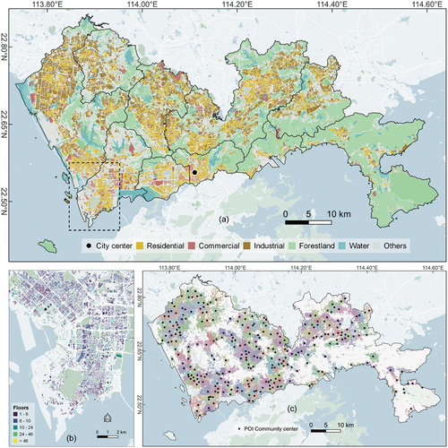
The POI dataset was created in January 2020 using the web service of Gaode Map, a map platform in China. By default, the service provides POI records in 22 level-1 categories. Here only 13 level-1 categories are included (see Table 1), while the other categories (e.g. vehicle maintenance and repair, location name and address, street ancillary facility, event and activity, etc.) that are considered irrelevant to the case study are dropped out from the dataset. Three processing procedures are implemented in the POI dataset. First, for a certain urban land unit, the numbers of POI in each category are summarized within the 500-m buffering area of that land unit. This procedure generates 13 additional attributes that collectively represent the neighborhood facility abundance for all urban land units. Second, the method proposed by Hidalgo et al. (2020) is applied to the POI dataset to generate 282 local communities (Figure 2(c)), which can somehow represent the locations of functional areas or submarkets (Tu et al. 2017). With the resulting communities, the attribute of Euclidean distance to the nearest community center is generated for all urban land units. Third, kernel density analysis is applied to the POI data, and the location with the highest density is manually selected as the location of city center. The attribute of Euclidean distance to city center can then be generated for all urban land units.

Table 1. POI categories and their corresponding attribute names.

Attribute names	POI categories
Type_5	Food/Beverages service
Type_6	Retailing/Wholesaling
Type_7	Life service
Type_8	Sport/Leisure site
Type_9	Hospital/Health care service
Type_10	Accommodation service
Type_11	Scenic spot
Type_12	Residential quarter/Office building
Type_13	Government agency and bureau
Type_14	Science/Education/Cultural facility
Type_15	Transport facility
Type_16	Finance and insurance service
Type_17	Company/Enterprise

To sum up, the maps and the dataset mentioned above generate the data to represent treatment (i.e. the land uses of residential, commercial, and industrial), outcomes (i.e. the mean building height), and attributes of land units. They are used to develop models of causal machine learning and estimate the causal effect of land use on building height.

3. Implementation and results

3.1. Preliminary analysis and settings for experiments

A descriptive summary of the data (Table 2) reveals that the mean building heights in residential, commercial, and industrial land are 8.40, 6.52, and 4.50 floors. However, these values do not suggest that the building height would increase by, for example, 2.02 (=6.52–4.50) floors on average if industrial land is changed to commercial land. This is simply because the difference between the mean floor counts for commercial land and industrial land is the result of both the noncausal effect and the causal effect induced by land use. Only by controlling the influences of the confounders, i.e. the attributes that affect both land use and building height, the actual causality of changing land use on building height can be captured.

Table 2. Mean and standard deviation of building heights in residential, commercial, and industrial land.

Building height in floor count	Residential	Commercial	Industrial
Mean	8.40	6.52	4.50
Standard deviation	5.95	5.31	2.41

Nevertheless, the comparison among the mean building heights can inspire the settings for experiments. Intuitively, one would expect that changing a certain piece of industrial land to residential land would lead to increased building height, although a specific increase is is yet to be estimated. Such an expectation is also consistent with actual experiences of urban (re)development. Therefore, in this study, three experiments are implemented to estimate the causal effect of land use. The total number of land units used for the experiments is 6529 (including 3511 residential land units, 2093 commercial land units, and 925 industrial land units). Specifically, Experiment #1 regards all residential land units as the treatment group (T = 1) and all industrial land units as the control group (T = 0). The number of land units used in Experiment #1 is 4436. This experiment is to estimate the causal effect on building height if a certain piece of industrial land is converted to residential land. Similarly, Experiment #2 is designed to estimate the causal effect on building height if a certain piece of industrial land is changed to commercial land, and hence regards all commercial land units as the treatment group (T = 1) and all industrial land units as the control group (T = 0). The number of land units used in Experiment #2 is 3018. Finally, Experiment #3 regards all residential land units as the treatment group (T = 1) and all commercial land units as the control group (T = 0), which is to estimate the change in building height caused by the land use change from commercial to residential. The number of land units used in Experiment #3 is 5604. All these experiments are carried out using the Python package of EconML developed by Microsoft Research (Syrgkanis et al. 2021). The following sections describe the results of these three experiments.

3.2. Model performance and sensitivity analysis

The selected models are fitted using the training data set (75% out of the full data set) and evaluated using the testing data set (25% out of the full data set). For all models, random forest is used for the required procedures of classification and regression because of the prevalence and the reliable performance reported in literature (Brenning 2022; Kang et al. 2022). The estimated ATE using the training data and the rscores computed using the testing data set are summarized in Table 3. Among the three experiments, there are two models that consistently yield negative rscores, namely BasicDML and R-Learner, indicating that these two models are overfitted. By contrast, the models of T-Learner and DALearner consistently yield the highest rscores as compared with others.

Table 3. ATE estimated by the selected models using the training data and their rscores (in the parentheses; scaled by 10⁻³) computed using the testing data set. The star sign indicates which models are used for ensemble.

Models	Experiment #1 (TResidential = 1 and TIndustrial = 0)	Experiment #2 (TComercial = 1 and TIndustrial = 0)	Experiment #3 (TResidential = 1 and TCommercial = 0)
T-Learner	3.59 (8.37)*	1.51 (3.37)*	2.54 (1.42)
S-Learner	3.58 (5.59)	0.14 (−9.63)	2.40 (4.83)
X-Learner	3.36 (3.56)	1.18 (−1.34)	2.58 (7.53)*
DALearner	3.67 (8.39)*	1.58 (4.48)*	2.58 (8.23)*
DRLearner	3.68 (5.43)	1.14 (−24.54)	2.63 (1.22)
BasicDML	2.45 (−7.32)	0.60 (−3.26)	2.07 (−2.78)
R-Learner	2.57 (−43.50)	1.00 (−72.66)	2.52 (−7.37)
Causal forest	3.01 (6.03)*	0.70 (−3.70)	2.39 (1.18)
Ensemble	3.60 (9.30)	1.57 (4.69)	2.58 (9.27)

With these results, model ensembles are further performed according to the rscores. Besides the reason that model ensemble usually can produce result better than the single best one, there is another important advantage to doing ensemble in this study: to alleviate the influences of randomness induced by training-and-testing data split. Because the rscores are computed using the testing data set, the specific results are influenced by how the whole dataset is split. That is, the specific results of the rscores may change if the testing dataset is changed. Despite that, the relative differences of rscores among the models are insensitive to the data used. For instance, in Experiment #1 (T_Residential = 1 and T_Industrial = 0), regardless of their specific rscore values, T-Learner and DALearner are always among the best models in different rounds of rscore computation using different sets of testing data. In such a case, it is more reasonable to combine all the “good” models rather than only picking a single “best” model, because that single “best” model may not always be the best when different sets of testing data are used.

The model ensemble procedure operates simply as trying different combinations of single models until the highest rscore is achieved with the minimum number of models. The models used for ensemble in each experiment are shown in Table 3 with the star sign. The results show that the model ensemble is effective in improving rscores. For instance, in Experiment #1 (T_Residential = 1 and T_Industrial = 0), the best estimate can be obtained by ensembling the model outcomes of T-Learner, DALearner, and causal forest. While in Experiment #2 (T_Comercial = 1 and T_Industrial = 0), the best estimate can be obtained by ensembling only the outcomes of T-Learner and DALearner; and in Experiment #3 (T_Residential = 1 and T_Comercial = 0), the models of X-Learner and DALearner are used to do ensemble. Moreover, model ensemble is more effective in improving the results in Experiments #1 (rscore = 9.30) and #3 (rscore = 9.27), in which the gains of rscore are 11% and 13%, respectively, as compared to the highest rscores of individual models (i.e. 8.39 in Experiment #1 and 8.23 in Experiment #3).

Sensitivity analysis is also applied to the finally selected models in each experiment. The results of the three tests are shown in Table 4. The p-values of all the models are insignificant (>0.05) in D_Subset and C_Random, suggesting that the null hypothesis (i.e. the estimated ATE and the new ATE after changing input data/adding a new cause are the same) cannot be rejected. Therefore, all models pass the tests of D_Subset and C_Random. In the test of T_Random, all models yield non-zero estimates after permutation, but the corresponding p-values are insignificant, suggesting that the null hypothesis (i.e. the new ATE is zero after permuting the treatment variable) cannot be rejected. Therefore, all models consistently pass the test of T_Random.

Table 4. Results of sensitivity analysis (p-values are shown in the parentheses).

	Estimated ATE	ATE-DSubset	ATE-CRandom	ATE-TRandom
Experiment #1
T-Learner	3.68	3.72 (0.44)	3.69 (0.40)	−0.17 (0.32)
DALearner	3.82	3.66 (0.22)	3.85 (0.13)	0.12 (0.30)
Causal forest	3.03	3.04 (0.49)	3.03 (0.48)	0.04 (0.42)
Experiment #2
T-Learner	1.73	1.64 (0.41)	1.73 (0.42)	−0.06 (0.45)
DALearner	1.78	1.71 (0.45)	1.75 (0.26)	0.16 (0.26)
Experiment #3
X-Learner	1.75	1.81 (0.41)	1.73 (0.32)	0.01 (0.49)
DALearner	1.70	1.54 (0.33)	1.65 (0.09)	0.08 (0.37)

D_Subset = analysis that uses a subset of data; C_Random = analysis that adds a random common cause; T_Random = analysis that uses a placebo treatment..

3.3. Interpretation of the heterogenous treatment effects

The ensembled models are applied to the data of industrial land and commercial land, generating the individual treatment effects for three counterfactual scenarios of land use change: from industrial use to residential use (Ind2Res), from industrial use to commercial use (Ind2Com), and from commercial use to residential use (Com2Res). The corresponding results of ATE are 3.68, 1.61, and 2.35 floors for Ind2Res, Ind2Com, and Com2Res. These results change marginally as compared with those obtained using the training data, suggesting that the models applied are reliable. The results are interpreted from spatial and factorial perspectives, with the former focusing on spatial patterns and the latter focusing on the heterogeneity of treatment effect.

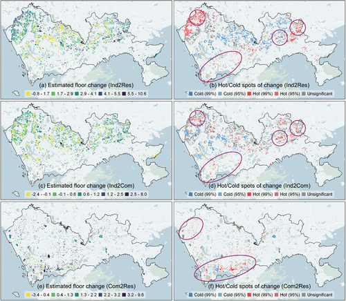
In addition to mapping the individual treatment effect, hot spot analysis is also implemented to recognize where greater building height change would occur (Figure 3). In Ind2Res scenario, only less than 1% of the industrial land units have negative treatment effects if land use is changed from industrial to residential, with a mean treatment effect of over 2.99 floors. In Ind2Com scenario, however, approximately 14% of the land units have negative treatment effects, with a mean treatment effect of only 0.65 floors. Notably, despite the difference in extent, several hot spots of building height increase in the scenarios of Ind2Res and Ind2Com overlap spatially (the solid ellipses in Figure 3(b–d), suggesting satisfactory conditions for either residential or commercial activities in these land units. In Com2Res, approximately 12% of the commercial land units have negative treatment effects if they are converted to residential land. The mean treatment effect is 1.87 floors. Most of the hot spots of building height change are within the central area of the city, owing mainly to the background characteristics of commercial land distribution, while other hot spots are located around those in Ind2Res scenario (the solid ellipses in Figure 3(f)).

Figure 3. The estimated change in the number of floors and the hot/cold spots of change for each scenario. The solid ellipses highlight the representative areas that are identified as the hot spots of building height change.

Moreover, by using the decision tree algorithm, the land units can be separated into different groups according to the values of their attributes. This procedure can visualize attribute importance and how the treatment effect varies in different groups of land units (Figure 4). The results reveal different conditions that can lead to greater building height change in each scenario. For instance, in Ind2Res scenario, there are three groups of land units that have treatment effects greater than the mean level. Specifically, group A represents the land units that are larger than 3001 m² and within the distance of 7–11 km to the city center. If land units are larger than 7021 m² and have a small number of companies/enterprises (≤107.5) in their neighborhood (i.e. group B), then the treatment effects would be even stronger. Otherwise, only if they have more abundant companies/enterprises (>107.5) in their neighborhood and are far from city center (>34 km) (i.e. group C), stronger treatment effects would be observed when they are converted to residential land.

Figure 4. Decision trees of the heterogeneous treatment effect in each scenario. CATE refers to conditional average treatment effect. Greener color indicates greater values of CATE, while redder color indicates smaller values of CATE.

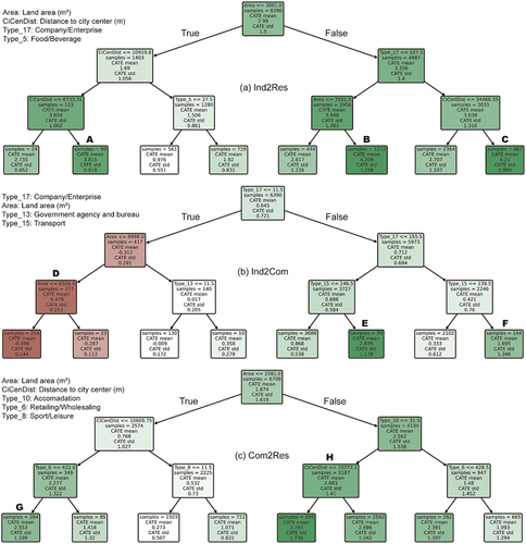
The results in Ind2Com scenario show divergent paths of treatment effects. The two branches starting at the root node clearly separate the groups of high and low treatment effects. The results suggest that the number of nearby companies/enterprises determines whether the treatment fails. If land units do not have enough companies/enterprises (≤11.5) in their neighborhood and are smaller than 6326 m² (i.e. group D), the treatment effects would become negative. By contrast, the results for groups E and F indicate that the abundance of transport facility is a key to stronger treatment effects. If the number of nearby transport facility is insufficient (e.g. ≤139.5), the treatment effects would be trivial (0.33 only) even though nearby companies/enterprises are abundant.

In Com2Res scenario, two attributes are found important to affect the treatment effects, namely distance to city center and neighborhood abundance of accommodation facility. Stronger treatment effects would be achieved if the commercial land units are small (≤2581 m²), close enough to the city center (≤11 km (Figure 4(c)), and have less retailing/wholesaling facilities in their neighborhood (i.e. group G). For bigger commercial land units (>2587 m²), however, stronger treatment effects would be achieved if they have less accommodation facilities in their neighborhood (≤31.5) (group H).

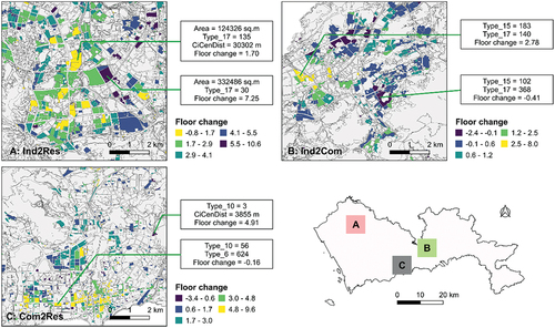
Figure 5 highlights three representative areas of heterogeneous treatment effects. Area A illustrates the floor change for two industrial parcels in the Ind2Res scenario. The major factor that differentiates the outcomes of floor change is the number of companies/enterprises (Type_17). The parcel with too many companies/enterprises nearby is expected to have a small floor change, as compared with the other parcel with far fewer companies/enterprises nearby. In area B for the Ind2Com scenario, the most influential determinants are the number of transport facility as well as the abundance of companies/enterprises. Greater floor change is expected to occur in the parcels with more transport facilities and fewer companies/enterprises. In the Com2Res scenario, the number of accommodation facility is the key factor that affects the treatment effect. As illustrated by the two examples in area C, the parcel with few accommodation facilities and a moderate distance away from the city center is expected to have a relatively large floor change. The parcel with many accommodation facilities and companies/enterprises nearby, however, is expected to have a marginal floor change.

Figure 5. Heterogeneous treatment effects in three representative areas.

4. Discussion

The presented results have demonstrated the usefulness of causal machine learning models to understand how building height would change if a certain type of land use change occurs, a question which is important for urban renewal but cannot be properly answered by conventional correlation-oriented models. Despite that the case study solely focuses on building height, other measures of urban development (e.g. rent) are also feasible for causal analysis, if relevant data are available. Nevertheless, building height is easy to observe, and also correlates with many other indicators of urban morphologies such as population density (Jedwab, Loungani, and Yezer 2021) and activity composition/concentration (Cai and Chen 2022). Therefore, the causality captured in this study is still helpful to inspire and evaluate urban development plans. In particular, causal machine learning models can unveil the heterogeneity of causality that, in this case study, suggests which group of land units are more effective to be developed in terms of building height change (Figure 3) and on what conditions such an intervention can be more successful (Figure 4).

This study also contributes to literature by complementing existing models of urban redevelopment. Urban redevelopment is more difficult to model often due to the insufficient observational data of actual redevelopment, as compared with the abundant observations of urban expansion/growth, which can be conveniently captured by satellites (X. Liu et al. 2020). This is partly because urban redevelopment often takes more time to occur due to the complex intertwined issues (e.g. legality, rights, goals, and so on) for negotiation. Furthermore, many studies that attempt to project future urban development (Y. Chen 2022; Wolff et al. 2020) have to comprise by ignoring or excluding the process of urban redevelopment from their models, making the projections somewhat unreasonable, especially if a declining urban population is expected (G. Chen et al. 2020; Miyauchi, Setoguchi, and Ito 2021). By integrating conventional urban models with the methods of cause analysis, however, urban redevelopment can be explicitly modeled and more reliable projections can be made.

Nevertheless, this study suffers from several limitations that can be addressed in the future. First, the presented case study does not take into account the costs and benefits of land use change. For instance, because of the higher costs, land units in the central area of the city may not always be considered as the first choice to (re)develop, even though they have greater returns as compared with other land units in the sub-urban area. If relevant data of costs and benefits are accessible, the causality and its heterogeneity can be better explained. Also, the land use data applied in this study do not exclude land units that had experienced changes induced by urban redevelopment. Although this issue would not affect too much the significance of the results, it would be better to exclude those land units from analysis if relevant data were available. Second, the presented study is indeed a causal analysis with spatial data rather than a realization of spatial causal reasoning. The spatial effect (e.g. spatial dependence, spatial trend, etc.) that could exist in the covariates, treatment, and outcomes have not been explicitly addressed, although the distance variables and the neighborhood conditions included in this study can to some extent reduce the geographic confounding. Therefore, another important task in the future work is to establish a more comprehensive framework that allows spatial causal reasoning. Third, although beyond the focus of this study, the causality captured in the case study has yet to be evaluated from the perspective of spatial-temporal modeling for urban (re)development, which is one of the important themes of GIScience and urban study as well.

5. Conclusion

This study uses causal machine learning models to infer the causality between land use and building height, which is relevant to urban renewal/redevelopment. A total of eight causal machine learning models are selected for causal effect estimation. The performances of these models are evaluated and compared. Models that perform well are further ensembled to produce more robust estimation.

The model ensembles suggest that building height would increase by 3.68 floors and 1.61 floors on average if industrial land is converted to residential and commercial, respectively, and 2.35 floors if commercial land is converted to residential land. The heterogeneity of causal effect is also captured and demonstrated for different scenarios of land use change. The spatial results feature some overlapping hot spots where a greater increase in building height would be observed if industrial land is either converted to residential land or commercial land. The factor analysis reveals several key rules that can lead to greater building height increase by changing land use. The models and results presented in this study are expected to better support policy-makers of urban renewal.

Future studies would focus on involving more attributes to improve the representation of heterogeneous causality, such as indicators of costs and benefits, factors of macro economy and regional development plan, etc. Also, the causal machine learning models applied in this study can be combined with conventional urban simulation models, thereby making more reliable projections for future development.

Disclosure statement

No potential conflict of interest was reported by the author(s).

Data availability statement

Data used in this study are available upon reasonable request to the corresponding author.

Additional information

Funding

This work was supported by the National Natural Science Foundation of China under Grant [number 42322110 and 42271415] and the Guangdong Natural Science Funds for Distinguished Young Scholar under Grant [number 2021B1515020104].

References

- Athey, S. 2015. “Machine Learning And Causal Inference For Policy Evaluation.” In Proceedings of the 21th ACM SIGKDD International Conference on Knowledge Discovery and Data Mining, Sydney NSW Australia, 5–16.
- Athey, S., and G. Imbens. 2016. “Recursive Partitioning For Heterogeneous Causal Effects.” Proceedings of the National Academy of Sciences 113 (27): 7353–7360. https://doi.org/10.1073/pnas.1510489113.
- Athey, S., J. TIbshirani, and S. Wager. 2019. “Generalized Random Forests.” The Annals of Statistics 47 (2): 1148–1178. https://doi.org/10.1214/18-AOS1709.
- Brenning, A. 2022. “Spatial Machine-learning Model Diagnostics: A Model-agnostic Distance-based Approach.” International Journal of Geographical Information Science 37 (3): 1–23. https://doi.org/10.1080/13658816.2022.2131789.
- Cai, J., and Y. Chen. 2022. “A Novel Unsupervised Deep Learning Method for the Generalization of Urban Form.” Geo-Spatial Information Science 25 (4): 568–587. https://doi.org/10.1080/10095020.2022.2068384.
- Cao, K., M. Batty, B. Huang, Y. Liu, L. Yu, and J. Chen. 2011. “Spatial Multi-Objective Land Use Optimization: Extensions to the Non-Dominated Sorting Genetic Algorithm-II.” International Journal of Geographical Information Science 25 (12): 1949–1969. https://doi.org/10.1080/13658816.2011.570269.
- Chen, Y. 2022. “An Extended Patch-Based Cellular Automaton to Simulate Horizontal and Vertical Urban Growth Under the Shared Socioeconomic Pathways.” Computers, Environment and Urban Systems 91:101727. https://doi.org/10.1016/j.compenvurbsys.2021.101727.
- Chen, Y., and M. Feng. 2022. “Urban Form Simulation in 3D Based on Cellular Automata and Building Objects Generation.” Building and Environment 226:109727. https://doi.org/10.1016/j.buildenv.2022.109727.
- Chen, G., X. Li, X. Liu, Y. Chen, X. Liang, J. Leng, X. Xu, et al. 2020. “Global Projections of Future Urban Land Expansion Under Shared Socioeconomic Pathways.” Nature Communications 11 (1): 537. https://doi.org/10.1038/s41467-020-14386-x.
- Chernozhukov, V., D. Chetverikov, M. Demirer, E. Duflo, C. Hansen, W. Newey, J. Robins, et al. 2018. “Double/Debiased Machine Learning for Treatment and Structural Parameters.” The Econometrics Journal 21 (1): C1–C68. https://doi.org/10.1111/ectj.12097.
- Clarke, K., and L. Gaydos. 1998. “Loose-Coupling a Cellular Automaton Model and GIS: Long-Term Urban Growth Prediction for San Francisco and Washington/Baltimore.” International Journal of Geographical Information Science 12 (7): 699–714. https://doi.org/10.1080/136588198241617.
- Cui, P. 2020. “Causal Inference Meets Machine Learning.” In Proceedings of the 26th ACM SIGKDD International Conference on Knowledge Discovery and Data Mining, New York, USA, 3527–3528.
- Cui, P., and S. Athey. 2022. “Stable Learning Establishes Some Common Ground Between Causal Inference and Machine Learning.” Nature Machine Intelligence 4 (2): 110–115. https://doi.org/10.1038/s42256-022-00445-z.
- Eikelboom, T., R. Janssen, and T. Stewart. 2015. “A Spatial Optimization Algorithm for Geodesign.” Landscape and Urban Planning 144:10–21. https://doi.org/10.1016/j.landurbplan.2015.08.011.
- Feng, Y., and X. Tong. 2020. “A New Cellular Automata Framework of Urban Growth Modeling by Incorporating Statistical and Heuristic Methods.” International Journal of Geographical Information Science 34 (1): 74–97. https://doi.org/10.1080/13658816.2019.1648813.
- Foster, D. J., and V. Syrgkanis. 2023. “Orthogonal Statistical Learning.” Annals of Statistics 51 (3): 879–908. https://doi.org/10.1214/23-AOS2258.
- Funderburg, R. G., H. Nixon, M. G. Boarnet, and G. Ferguson. 2010. “New Highways and Land Use Change: Results from a Quasi-Experimental Research Design.” Transportation Research Part A: Policy and Practice 44 (2): 76–98. https://doi.org/10.1016/j.tra.2009.11.003.
- Hagenauer, J., H. Omrani, and M. Helbich. 2019. “Assessing the Performance of 38 Machine Learning Models: The Case of Land Consumption Rates in Bavaria, Germany.” International Journal of Geographical Information Science 33 (7): 1399–1419. https://doi.org/10.1080/13658816.2019.1579333.
- Hewitt, R. J., M. Shadmanroodposhti, and B. A. Bryan. 2022. “There’s No Best Model! Addressing Limitations of Land-Use Scenario Modelling Through Multi-Model Ensembles.” International Journal of Geographical Information Science 36 (12): 2352–2385. https://doi.org/10.1080/13658816.2022.2098299.
- Hidalgo, C. A., E. Castañer, and A. Sevtsuk. 2020. “The Amenity Mix of Urban Neighborhoods.” Habitat International 106:102205. https://doi.org/10.1016/j.habitatint.2020.102205.
- Imbens, G. W., and D. B. Rubin. 2015. Causal Inference in Statistics, Social, and Biomedical Sciences. New York, USA: Cambridge University Press.
- Jacob, D. 2021. “CATE Meets ML: Conditional Average Treatment Effect and Machine Learning.” Digital Finance 3 (2): 99–148. https://doi.org/10.1007/s42521-021-00033-7.
- Jedwab, R., P. Loungani, and A. Yezer. 2021. “Comparing Cities in Developed and Developing Countries: Population, Land Area, Building Height and Crowding.” Regional Science and Urban Economics 86:103609. https://doi.org/10.1016/j.regsciurbeco.2020.103609.
- Jones, K. W., D. J. Lewis, and M. S. Crowther. 2015. “Estimating the Counterfactual Impact of Conservation Programs on Land Cover Outcomes: The Role of Matching and Panel Regression Techniques.” Public Library of Science ONE 10 (10): e0141380. https://doi.org/10.1371/journal.pone.0141380.
- Kang, M., Y. Liu, M. Wang, L. Li, and M. Weng. 2022. “A Random Forest Classifier with Cost-Sensitive Learning to Extract Urban Landmarks from an Imbalanced Dataset.” International Journal of Geographical Information Science 36 (3): 496–513. https://doi.org/10.1080/13658816.2021.1977814.
- Künzel, S. R., J. S. Sekhon, P. J. Bickel, and B. Yu. 2019. “Metalearners for Estimating Heterogeneous Treatment Effects Using Machine Learning.” Proceedings of the National Academy of Sciences 116 (10): 4156–4165. https://doi.org/10.1073/pnas.1804597116.
- Lecca, P. 2021. “Machine Learning for Causal Inference in Biological Networks: Perspectives of This Challenge.” Frontiers in Bioinformatics 1:746712. https://doi.org/10.3389/fbinf.2021.746712.
- Lechner, T. 2018. Domain Adaptation Under Causal Assumptions. Tübingen, Germany: Eberhard Karls Universität Tübingen Tübingen.
- Leist, A. K., M. Klee, J. H. Kim, D. H. Rehkopf, S. P. A. Bordas, G. Muniz-Terrera, and S. Wade. 2022. “Mapping of Machine Learning Approaches for Description, Prediction, and Causal Inference in the Social and Health Sciences.” Science Advances 8 (42): eabk1942. https://doi.org/10.1126/sciadv.abk1942.
- Li, B. 2022. “Prospects on Causal Inferences in GIS.” In New Thinking in GIScience, edited by B. Li, X. Shi, A-X. Zhu, C. Wang, and H. Lin, 109–118. Singapore, Singapore: Springer.
- Liu, Y., M. Batty, S. Wang, and J. Corcoran. 2021. “Modelling Urban Change with Cellular Automata: Contemporary Issues and Future Research Directions.” Progress in Human Geography 45 (1): 3–24. https://doi.org/10.1177/0309132519895305.
- Liu, X., Y. Huang, X. Xu, X. Li, X. Li, P. Ciais, P. Lin, et al. 2020. “High-Spatiotemporal-Resolution Mapping of Global Urban Change from 1985 to 2015.” Nature Sustainability 3 (7): 564–570. https://doi.org/10.1038/s41893-020-0521-x.
- Liu, X., X. Liang, X. Li, X. Xu, J. Ou, Y. Chen, S. Li, et al. 2017. “A Future Land Use Simulation Model (FLUS) for Simulating Multiple Land Use Scenarios by Coupling Human and Natural Effects.” Landscape and Urban Planning 168:94–116. https://doi.org/10.1016/j.landurbplan.2017.09.019.
- Liu, Y., A.-X. Zhu, J. Wang, W. Li, G. Hu, and Y. Hu. 2019. “Land-Use Decision Support in Brownfield Redevelopment for Urban Renewal Based on Crowdsourced Data and a Presence-And-Background Learning (PBL) Method.” Land Use Policy 88:104188. https://doi.org/10.1016/j.landusepol.2019.104188.
- Li, X., and A. G. O. Yeh. 2001. “Calibration of Cellular Automata by Using Neural Networks for the Simulation of Complex Urban Systems.” Environment and Planning A 33 (8): 1445–1462. https://doi.org/10.1068/a33210.
- Li, X., and A. G. O. Yeh. 2004. “Data Mining Of Cellular Automata’s Transition Rules.” International Journal of Geographical Information Science 18 (8): 723–744. https://doi.org/10.1080/13658810410001705325.
- Lu, Y., S. Laffan, C. Pettit, and M. Cao. 2020. “Land Use Change Simulation and Analysis Using a Vector Cellular Automata (CA) Model: A Case Study of Ipswich City, Queensland, Australia.” Environment & Planning B: Urban Analytics & City Science 47 (9): 1605–1621. https://doi.org/10.1177/2399808319830971.
- Magliocca, N. R., P. Dhungana, and C. D. SInk. 2023. “Review of Counterfactual Land Change Modeling for Causal Inference in Land System Science.” Journal of Land Use Science 18 (1): 1–24. https://doi.org/10.1080/1747423X.2023.2173325.
- Meng, L., Y. Sun, and S. Zhao. 2020. “Comparing the Spatial and Temporal Dynamics of Urban Expansion in Guangzhou and Shenzhen from 1975 to 2015: A Case Study of Pioneer Cities in China’s Rapid Urbanization.” Land Use Policy 97:104753. https://doi.org/10.1016/j.landusepol.2020.104753.
- Meyfroidt, P. 2016. “Approaches and Terminology for Causal Analysis in Land Systems Science.” Journal of Land Use Science 11 (5): 501–522. https://doi.org/10.1080/1747423X.2015.1117530.
- Meyfroidt, P., A. de Bremond, C. M. Ryan, E. Archer, R. Aspinall, A. Chhabra, G. Camara, et al. 2022. “Ten Facts About Land Systems for Sustainability.” Proceedings of the National Academy of Sciences 119 (7): e2109217118. https://doi.org/10.1073/pnas.2109217118.
- Millington, J. D., D. O’sullivan, and G. L. Perry. 2012. “Model Histories: Narrative Explanation In Generative Simulation Modelling.” Geoforum; Journal of Physical, Human, and Regional Geosciences 43 (6): 1025–1034. https://doi.org/10.1016/j.geoforum.2012.06.017.
- Miyauchi, T., T. Setoguchi, and T. Ito. 2021. “Quantitative Estimation Method for Urban Areas to Develop Compact Cities in View of Unprecedented Population Decline.” Cities 114:103151. https://doi.org/10.1016/j.cities.2021.103151.
- Nie, X., and S. Wager. 2021. “Quasi-Oracle Estimation of Heterogeneous Treatment Effects.” Biometrika 108 (2): 299–319. https://doi.org/10.1093/biomet/asaa076.
- Nugroho, N. Y., S. Triyadi, and S. Wonorahardjo. 2022. “Effect of High-Rise Buildings on the Surrounding Thermal Environment.” Building and Environment 207:108393. https://doi.org/10.1016/j.buildenv.2021.108393.
- Patel, P., S. Karmakar, S. Ghosh, and D. Niyogi. 2020. “Improved Simulation of Very Heavy Rainfall Events by Incorporating WUDAPT Urban Land Use/Land Cover in WRF.” Urban Climate 32:100616. https://doi.org/10.1016/j.uclim.2020.100616.
- Pettit, C., S. Biermann, C. Pelizaro, and A. Bakelmun. 2020. “A Data-Driven Approach to Exploring Future Land Use and Transport Scenarios: The Online What If? Tool.” Journal of Urban Technology 27 (2): 21–44. https://doi.org/10.1080/10630732.2020.1739503.
- Pontius, R. G., JR, J. D. Cornell, and C. A. Hall. 2001. “Modeling the Spatial Pattern of Land-Use Change with GEOMOD2: Application and Validation for Costa Rica.” Agriculture, Ecosystems and Environment 85 (1–3): 191–203. https://doi.org/10.1016/S0167-8809(01)00183-9.
- Rudin, C. 2019. “Stop Explaining Black Box Machine Learning Models for High Stakes Decisions and Use Interpretable Models Instead.” Nature Machine Intelligence 1 (5): 206–215. https://doi.org/10.1038/s42256-019-0048-x.
- Said, M., C. Hyandye, H. C. Komakech, I. C. Mjemah, and L. K. Munishi. 2021. “Predicting Land Use/Cover Changes and Its Association to Agricultural Production on the Slopes of Mount Kilimanjaro, Tanzania.” Annals of GIS 27 (2): 189–209. https://doi.org/10.1080/19475683.2020.1871406.
- Sanchez, P., J. P. Voisey, T. Xia, H. I. Watson, A. Q. O’Neil, and S. A. Tsaftaris. 2022. “Causal Machine Learning for Healthcare and Precision Medicine.” Royal Society Open Science 9 (8): 220638. https://doi.org/10.1098/rsos.220638.
- Schuler, A.,Baiocchi, M., Tibshirani, R. and Shah, N. 2018. “A Comparison of Methods for Model Selection When Estimating Individual Treatment Effects.” ArXiv Preprint 1804:05146. https://doi.org/10.48550/arXiv.1804.05146.
- Sharma, A., and E. KIciman. 2020. “Dowhy: An End-to-end Library For Causal Inference.” ArXiv Preprint. https://doi.org/10.48550/arXiv.2011.04216.
- Syrgkanis, V., Lewis, G., Oprescu, M., Hei, M., Battocchi, K., Dillon, E., Pan, J., Wu, Y., Lo, P., Chen, H. and Harinen, T. 2021. “Causal Inference and Machine Learning in Practice with Econml and Causalml: Industrial Use Cases at Microsoft, Tripadvisor, Uber.” In Proceedings of the 27th ACM SIGKDD Conference on Knowledge Discovery and Data Mining, New York, USA, 4072–4073.
- Tu, W., J. Cao, Y. Yue, S.-L. Shaw, M. Zhou, Z. Wang, X. Chang, et al. 2017. “Coupling Mobile Phone and Social Media Data: A New Approach to Understanding Urban Functions and Diurnal Patterns.” International Journal of Geographical Information Science 31 (12): 2331–2358. https://doi.org/10.1080/13658816.2017.1356464.
- Verburg, P. H., and K. P. Overmars. 2009. “Combining Top-Down and Bottom-Up Dynamics in Land Use Modeling: Exploring the Future of Abandoned Farmlands in Europe with the Dyna-CLUE Model.” Landscape Ecology 24 (9): 1167–1181. https://doi.org/10.1007/s10980-009-9355-7.
- Wager, S., and S. Athey. 2018. “Estimation and Inference of Heterogeneous Treatment Effects Using Random Forests.” Journal of the American Statistical Association 113 (523): 1228–1242. https://doi.org/10.1080/01621459.2017.1319839.
- Wang, W., D. Wang, H. Chen, B. Wang, and X. Chen. 2022. “Identifying Urban Ventilation Corridors Through Quantitative Analysis of Ventilation Potential and Wind Characteristics.” Building and Environment 214:108943. https://doi.org/10.1016/j.buildenv.2022.108943.
- Wolff, C., T. Nikoletopoulos, J. Hinkel, and A. T. Vafeidis. 2020. “Future Urban Development Exacerbates Coastal Exposure In The Mediterranean.” Scientific Reports 10 (1): 1–11. https://doi.org/10.1038/s41598-020-70928-9.
- Zhai, Y., Y. Yao, Q. Guan, X. Liang, X. Li, Y. Pan, H. Yue, et al. 2020. “Simulating Urban Land Use Change by Integrating a Convolutional Neural Network with Vector-Based Cellular Automata.” International Journal of Geographical Information Science 34 (7): 1475–1499. https://doi.org/10.1080/13658816.2020.1711915.
- Zhang, H., X. Li, X. Liu, Y. Chen, J. Ou, N. Niu, Y. Jin, et al. 2019. “Will the Development of a High-Speed Railway Have Impacts on Land Use Patterns in China?” Annals of the American Association of Geographers 109 (3): 979–1005. https://doi.org/10.1080/24694452.2018.1500438.