Multivariate analysis of land surface dynamics in Central Asia: patterns of trends and drivers under a changing climate

ABSTRACT

With temperatures in Central Asia (CA) increasing more than the global average, this region is one of the global hotspots affected by climate change. CA is mostly characterized by arid climate, which is why available water resources are of paramount importance for the societies, economies, and the environment. In this regard, quantifying changes on the land surface and controlling factors that influence land surface dynamics are of great interest to improve our understanding of climate change impacts in this region. Hence, this study analyzes multivariate time series covering climatic, hydrological and Earth observation (EO)-based land surface variables. The used EO time series characterize the land surface and include data on the normalized difference vegetation index (NDVI), surface water area (SWA), and snow cover area (SCA) between December 2002 to November 2021. To analyze these time series, we employ trend analyses and a causal discovery algorithm. Both analyses were carried out at multiple spatial and temporal scales. The results show that NDVI trends were mostly significantly negative in the Northwest and positive in the Northeast of CA in summer. In summer and autumn, the percentage of significant negative NDVI trends outweighed the positive trends. For SWA, the detected trends were mostly significant negative throughout all scales. Significant negative trends were retrieved for SCA across all seasons, except for autumn regionally. Particularly the Tian Shan and Pamir mountains show significant declines of SCA in winter and spring. The causal analyses revealed that the NDVI is mostly controlled by water availability in summer. In spring and autumn, temperature is the leading driver on the NDVI. Likewise, temperature is found to largely control SWA in spring and autumn. SCA is mostly negatively coupled to temperature during spring and autumn. A positive coupling between SCA and precipitation is identified in winter.

KEYWORDS:

• Multivariate time series
• vegetation
• surface water area
• snow cover area
• trends and causality

1. Introduction

Central Asia (CA) is among the driest regions worldwide, and in times of amplified global climate warming the availability of freshwater has a crucial role for a sustainable development of the societies, economies, and the environment in this region. Concerning climate change in dryland areas, a particular high risk for warming temperatures over the next decades was reported by Huang et al. (2017). Also, the Intergovernmental Panel on Climate Change (IPCC) emphasized that CA will be dramatically influenced by climate warming compared to other regions in the world (IPCC 2018). In this context, investigations pointed toward a decreasing trend in precipitation since the end of the previous century and an intensification in warming temperatures over CA (Z. Hu et al. 2016; W. Zhang et al. 2021). Additionally, Hu and Han (2022) identified an expansion of desert climate in northern direction and particularly warming temperatures in cold regions of CA. On the contrary, increases in summer precipitation were found for the mountainous regions of CA by Meng et al. (2021). Also, future climate projections indicated an increase in extreme precipitation events that will result in more annual precipitation (Yao et al. 2021). An increase in the frequency and intensity of droughts over CA is expected as well (Ren et al. 2022).

In the light of these findings, Vakulchuk et al. (2022) emphasized the comparatively low availability of research related to climate change impacts in CA compared to other regions in Asia as well as the importance of recent investigations to support climate adaptation strategies. The limited availability of research on land surface variables in CA, including surface water resources, was also stated by Huang et al. (2021b). To contribute to a better understanding of environmental change and impacts of climatic factors on the land surface in CA, a multivariate feature space encompassing diverse spheres of the Earth system needs to be generated and analyzed. In this regard, remote sensing data characterizes the state of the land surface and allows for the generation of consistent time series over large areas to analyze changes on the land surface (Mahecha et al. 2020; Uereyen et al. 2022). More specifically, remote sensing time series might describe land surface variables, including features of vegetation, soil, surface water, snow cover, and glaciers. A prominent remote sensing instrument providing multispectral imagery for dense time series analysis are the Moderate Resolution Imaging Spectroradiometer (MODIS) sensors. These sensors collect medium spatial resolution data at daily temporal resolution since the year 2000 and thus enable the calculation of trends for land surface variables over two decades. In addition to trend calculation, multivariate time series, including climatic time series can be used to evaluate relations across different spheres of the Earth system. This type of analysis allows for the determination of controlling factors on land surface variables, such as vegetation health or the state of surface water area (SWA) and snow cover area (SCA). Available studies over CA analyzed the trends or controlling factors on single land surface variables such as the normalized difference vegetation index (NDVI) (e.g. Ding et al. (2022); Hao et al. (2022); Huang et al. (2021a)), SWA (e.g. Huang et al. (2021b); Liu et al. (2019); Yang et al. (2020)), and SCA (e.g. Ackroyd et al. (2021); Deng et al. (2021); Gulakhmadov et al. (2021); Tang et al. (2020)). In this context, the trend analyses are often conducted at annual scale lacking the detailed analysis at seasonal and mostly at pixel scale as well (e.g. Hao et al. (2022)) or the analyses were performed for subregions of CA only (e.g. Ding et al. (2022); Yang et al. (2020)). Furthermore, studies generally use correlation or residual analysis (e.g. Deng et al. (2021); Huang et al. (2021b)) to estimate controlling factors of a land surface variable. However, when applying correlation analyses the results might be spurious and the calculated correlation coefficient does not indicate a direction of influence between the used variables. The application of causal discovery algorithms can resolve these issues (e.g. Granger (1969); Papagiannopoulou et al. (2017); Runge et al. (2019a); Runge et al. (2019b)). The causal discovery algorithm Peter and Clark Momentary Conditional Independence (PCMCI) enables the analysis of a high dimensional feature space and serially correlated time series to infer direct and indirect links between a set of univariate time series (Runge, Bathiany, et al. 2019; Runge, Nowack, et al. 2019). PCMCI calculates causal process graphs to estimate interdependencies between the used time series at past temporal lags (Runge 2018). Considering the analysis of land surface dynamics over CA, PCMCI could enable the quantitative analysis of the relationship across multiple spheres of the Earth system, including the biosphere, hydrosphere, cryosphere, as well as atmosphere, and thus, contribute to a better understanding of land surface processes. In this context, a joint analysis of interdependencies between multiple remote sensing-based land surface variables and climatic drivers at seasonal and annual temporal scale as well as at different spatial scales using the causal discovery algorithm PCMCI is lacking so far for CA.

The overall aim of this study is to analyze land surface dynamics in CA from multiple perspectives. For this purpose, multivariate geoscientific time series that represent multiple spheres were employed. These include remote sensing-based time series on the land surface variables NDVI, SWA, and SCA in combination with climatic and hydrological time series for CA between the period December 2002 and November 2021. The aforementioned land surface variables were selected, since they are all based on MODIS data. In detail, the main objectives of this investigation are (1) to analyze seasonal and annual trends of the time series variables, (2) to estimate direct and indirect controls on the land surface variables, and (3) to explore spatiotemporal patterns in trends and drivers of the land surface variables in the light of amplified climate warming.

2. Materials and methods

2.1. Study area

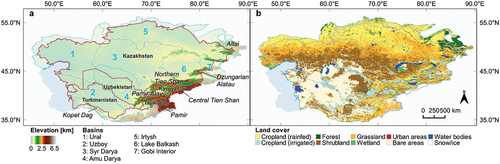
CA is located in the south of the Eurasian continent and includes the countries Kazakhstan, Uzbekistan, Turkmenistan, Kyrgyzstan, and Tajikistan (Figure 1) covering an area of approximately 3.9 million km². As illustrated in Figure 1, the elevation in CA increases from west to southeast, specifically from the Caspian Sea to the Pamir and Tian Shan mountains. The landscape of CA is characterized by plains and extensive steppe as well as desert areas. Rivers providing the western plains with freshwater originate in the southeastern mountains, in particular the rivers Amur Darya and Syr Darya. Furthermore, tributaries of the river Ob, specifically the Irtysh river are found in the northern areas of Kazakhstan, whereas the delta of the river Ural is in the Northwest of Kazakhstan. Besides river basins, Lake Balkash is a large endorheic basin in CA. Moreover, the climate in CA is dominated by steppe and desert climate being arid to semiarid at low altitudes as well as by cold and polar climate at high altitudes (Beck et al. 2018). The precipitation and temperature are characterized by a gradient from north to south as well as from low to high elevations. The precipitation is lowest in the South and in lowlands, whereas the mean annual temperature is highest in the South of CA (W. Zhang et al. 2021). As illustrated in Figure 1, croplands in CA are distinguished between rainfed and irrigated fields. Rainfed croplands can be found in Northern Kazakhstan and mountainous regions in the Southeast of CA. On the contrary, irrigated fields are located mostly in low-elevation and arid regions of CA. Considering the climate and growing season of this region, the following meteorological seasons are considered for the time series analyses at seasonal scale: winter (December, January, February), spring (March, April, May), summer (June, July, August), and autumn (September, October, November).

Figure 1. Characteristics of the study area showing (a) Copernicus Digital Elevation Model (DEM) (European Space Agency and Sinergise 2021) including outlines of the administrative boundaries as well as river basins (Lehner, Verdin, and Jarvis 2008) and (b) simplified land cover classification for 2019 over CA by means of the European Space Agencies (ESA) Climate Change Initiative (CCI) (European Space Agency 2017).

2.2. Time series variables

All used time series that characterize the land surface as well as climatic and hydrological variables are listed in Table 1. In this study, the land surface variables include vegetation, SWA, and SCA. Based on the timely overlap of the used time series, the investigated period was defined to cover December 2002 to November 2021. All daily time series are aggregated to biweekly intervals to minimize data gaps.

Table 1. Properties of the used time series and auxiliary data.

	Temporal	Temporal	Spatial
Used data	coverage	resolution	resolution [km]	Citation
MODIS Surface Reflectance (NDVI)	2000–present	Daily	0.50	Vermote and Wolfe (2015)
DLR Global SnowPack	2000–present	Daily	0.50	Dietz et al. (2015)
DLR Global WaterPack	2002–present	Daily	0.25	Klein et al. (2017)
ERA5-Land Variables	1950–present	Hourly	10.00	Muñoz-Sabater (2019)
GloFAS-ERA5 River Discharge	1979–present	Daily	10.00	Harrigan et al. (2020)
ESA CCI Land Cover	1992–2020	Yearly	0.30	European Space Agency (2017)
Copernicus Digital Elevation Model	2011–2015	–	0.03	European Space Agency, and Sinergise (2021)
HydroSHED	–	–	Vector	Lehner and Grill (2013)

2.2.1. Vegetation

To characterize vegetated areas, NDVI composites were calculated based on Terra and Aqua MODIS surface reflectance data. Using observations from both MODIS sensors allows to create consistent and high-quality measurements. In this regard, MODIS quality flags were utilized to remove pixels influenced by snow, cloud cover, and shadow. Since the quality assurance layers are provided at 1 km spatial resolution, the daily surface reflectance products were resampled to this spatial resolution. In a next step, the daily MODIS time series from the Terra and Aqua sensors were separately aggregated to biweekly composites using the median of all respective daily measurements. With this temporal aggregation, we aimed to minimize the impact of outliers. Afterwards, the composites for both sensors were merged by calculating their average for the respective biweekly interval. Available gaps in the NDVI time series were interpolated using a linear approach. To exclude non-vegetation pixels, all NDVI pixels with a long-term mean lower than 0.15 were excluded as applied, e.g. by Sarmah et al. (2018).

2.2.2. Surface water area

The analysis of SWA dynamics was conducted by means of the daily DLR Global WaterPack time series (Klein et al. 2017). In detail, the SWA time series is based on daily MODIS data at 250 m spatial resolution. Due to its high temporal and medium spatial resolution, this time series enables the detailed exploitation of SWA dynamics at large spatial scales. However, despite the high temporal resolution, the GWP might underestimate inland water bodies or river streams due to the relative coarse spatial resolution and resulting in mixed pixels. In this regard, high sediment load impacting the water color might result in an underestimation of water bodies. Yet, this dataset was applied in numerous studies to analyze e.g. trends and phenological characteristics of SWA (Klein et al. 2021; Uereyen et al. 2022; Uereyen, Bachofer, and Kuenzer 2022) and overcomes temporal gaps that result when using data at higher spatial resolution.

2.2.3. Snow cover area

To analyze snow cover area dynamics, the Global SnowPack data, which is generated at the German Aerospace Center (DLR) was employed (Dietz, Kuenzer, and Dech 2015). This dataset is based on daily MODIS snow data at a spatial resolution of 500 m and thus, allows for the aggregation to biweekly intervals. To process the gap-free DLR Global SnowPack, Dietz et al. (2015) used a dedicated processing chain to interpolate pixels that are e.g. contaminated by clouds. Furthermore, we excluded all snow pixels in the time series having a long-term mean less than 10% in order to minimize artifacts caused by cloud cover and ephemeral snow as applied by Notarnicola (2020a). Additionally, SCA was limited to areas above 1.500 m elevation to consider mountainous regions only. For this purpose, the Copernicus DEM was used (European Space Agency, & Sinergise 2021).

2.2.4. Climatic and hydrological variables

To evaluate the impacts of climatic and hydrological variables on the land surface, ERA5-Land reanalysis data from the European Centre for Medium Range Weather Forecasts (ECMWF) were utilized (Muñoz-Sabater 2019). These reanalysis data come at an enhanced spatial resolution of approximately 9 km and an hourly temporal resolution which allows for the calculation of time series at biweekly intervals. First, the daily accumulated feature values were retrieved from the hourly data of precipitation and surface solar radiation downward. In addition, 2-m air temperature, soil moisture (7–28 cm), and 2-m dew-point temperature were averaged to daily temporal scale. Furthermore, the variable vapor pressure deficit was calculated using temperature and dew-point temperature by means of the equation in Barkhordarian et al. (2019). Considering the performance of ERA5, Bhattacharya et al. (2021) show that temperature trends based on ERA5-Land result in high agreement with local observations in High Mountain Asia. Also, further studies emphasized the suitability of climatic variables from ERA5 in CA (e.g. Hu and Han (2022); Rakhmatova et al. (2021); Yu et al. (2023); Zandler et al. (2020)). With respect to solar radiation, Urraca et al. (2018) and Yang and Bright (2020) indicated a good performance of ERA5 compared to other data. Ultimately, to characterize river discharge the GloFAS-ERA5 gridded global river discharge v3.1 time series data (Harrigan et al. 2020) was employed. In this regard, it needs to be emphasized that the modeled river discharge has not been validated over the investigated study area. However, a validation of this data with globally distributed observations indicated a good performance (Harrigan et al. 2020).

2.2.5. Auxiliary data

Further data was used for the preprocessing of the time series, including the Copernicus Digital Elevation Model (DEM) (European Space Agency, & Sinergise 2021). The spatial extent of the basins was determined using the HydroSHED data (Lehner and Grill 2013; Lehner, Verdin, and Jarvis 2008). Land cover data was obtained from the European Space Agencies (ESA) Climate Change Initiative (CCI) (European Space Agency 2017). This data was used to analyze vegetation trends for different classes, including forest, grassland, irrigated cropland, and rainfed cropland. For this analysis, only stable land cover pixels between 2002 and 2020 were considered.

2.3. Methods

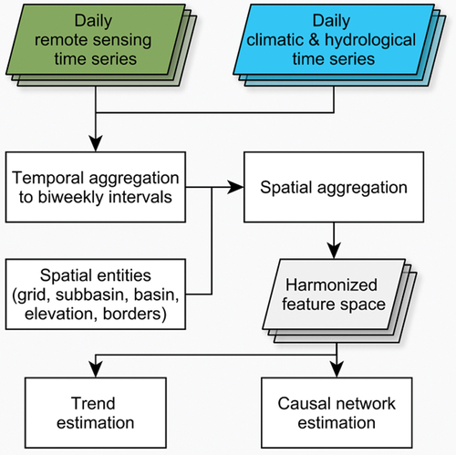
The multivariate analyses require the multi-source time series to be harmonized in terms of their spatial and temporal resolution. For this purpose, a uniform grid having a spatial resolution of 0.1° was introduced. In addition, geographic entities such as hydrological basins, national borders, and elevation zones were used for spatial harmonization in order to evaluate the trends for natural and anthropogenic units. Figure 2 briefly presents the applied workflow. More detailed information on the harmonization are available in Uereyen et al. (2022a).

Figure 2. Simplified overview of the time series harmonization and the application of the trend and causal discovery algorithm.

2.3.1. Calculation of trends

In this study, the linear trend of the investigated time series was calculated using the non-parametric Mann-Kendall test in combination with the Theil-Sen slope estimator (Kendall 1975; Mann 1945; Theil 1992). To account for serial correlation, the time series were prewhitened if serial correlation at lag-1 was statistically significant at a confidence level of 95%. Next to the prewhitening, the trend metrics were calculated. In this regard, the performed analysis did not rely on only one prewhitening approach as suggested by Collaud Coen et al. (2020) and Wang et al. (2015). To assess the statistical significance of the trends, the trend-free prewhitening algorithm after Wang and Swail (2001) was utilized. On the other hand, the variance corrected prewhitening approach after Wang et al. (2015) was used to estimate the magnitude of the trends. Furthermore, the trend tests were conducted at seasonal as well as annual scale at different spatial scales. The trend metrics are first calculated for the seasons winter, spring, summer, and autumn. For this calculation, the biweekly temporal resolution was used as it resulted in a higher number of data points. Here, the availability of a larger data sample improves the power of the trend tests (Collaud Coen et al. 2020). Afterwards, the annual trends were calculated using the median of the seasonal trends. Resulting trends were only considered, if they were statistically significant at a confidence level of 95%. In case of an insignificant trend, it was considered as a tendency. Also, it has to be noted that all trends were retrieved at decadal scale.

2.3.2. Evaluation of drivers of land surface variables

To identify drivers of the land surface variables NDVI, SWA, as well as SCA, and to analyze interdependencies in a multivariate feature space, the PCMCI+ algorithm was utilized (Runge 2020; Runge, Nowack, et al. 2019). This algorithm allows for the detection of contemporaneous (lag 0) and lagged relationships for a set of multiple variables. More specifically, the causal discovery algorithm PCMCI+ constructs causal networks, where the nodes depict the present variables and the edges the presence and direction of the detected causal relation among the variables. PCMCI employs a two-step procedure to identify linear or non-linear causal links, being a version of the Peter and Clark (PC) algorithm and the momentary conditional independence (MCI) test, which is applied using a conditional independence test. In this study, the linear partial correlation option was employed.

To explore the links of the multivariate time series, we created a unique feature space for each of the land surface variable NDVI, SWA, and SCA including relevant driving variables, respectively. The use time series with a high temporal resolution could improve the detection of causal links, which might potentially disappear at a aggregated resolution of, e.g., one month or season. Moreover, temporal lags were considered up to a maximum time lag of three months as suggested by Wu et al. (2015). This corresponds to six time steps at biweekly scale. To analyze the dependencies, PCMCI requires stationary time series (Runge, Nowack, et al. 2019). To this end, the linear trend of the time series was removed and seasonal anomalies were calculated using the approach presented in Uereyen et al. (2022a). In addition, to fulfill of the causal stationarity assumption, the mask option within the PCMCI framework, which splits the time series to defined seasons was utilized. Regarding the NDVI, the time series was limited to the growing season considering only seasons having an average NDVI greater than 0.15 and temperature greater than 0°C as suggested by Wu et al. (2015). Moreover, we quantified indirect influences on the land surface variables NDVI, SWA, and SCA at subbasin scale to illustrate the causal links as causal graphs. In total, we considered 171 subbasins over the study area and all time series were spatially aggregated at subbasin scale for calculating the causal graphs. In this context, we first spatially intersected all driving variables with the respective land surface variable and then computed causal graphs. The intersection step i.e. excluded non-vegetated areas for all of the considered driving variables from the analysis. Further details on the used parameters and settings can be found in Uereyen et al. (2022a).

3. Results

3.1. Multivariate time series

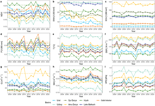
Figure 3 shows temporally and spatially averaged time series at annual and basins scale, respectively. Considering the NDVI, the average NDVI is highest in the Irtysh and lowest in the Uzboy river basin (Figure 3(a)). Each investigated river basin is characterized by certain fluctuations. In addition, between 2019 and 2021 there is a considerable decrease in the NDVI in all basins. Moreover, there is a negative peak in NDVI, vapor pressure deficit, and soil moisture in the Amu Darya and Uzboy river basins during the year 2008. Regarding the SWA time series, a constant decline in the Amu Darya river basin is prominent (Figure 3b). In addition, there are distinct anomalies present in the SWA time series. Furthermore, anomalies in SCA appear to be associated with temperature and precipitation, particularly in the Amu Darya river basin in the years 2008 and 2009. For example, precipitation and SCA are both characterized by negative anomalies in 2008 and positive anomalies in 2009 (Figure 3c,d).

Figure 3. Annually aggregated time series at basin scale between the years 2003 and 2021. The time series long-term mean is indicated by the dashed lines. Abbreviations: (a) Normalized difference vegetation index (NDVI), (b) surface water area (SWA), (c) snow cover area (SCA), (d) precipitation (P), (e) temperature (T), (f) downward shortwave solar radiation (DSR), (g) river discharge (Q), (h) soil moisture (SM), (i) vapor pressure deficit (VPD).

3.2. Trends at basin scale

Table 2 lists the calculated trends for all investigated time series at basin and annual as well as seasonal scale. In detail, the NDVI showed barely significant trends at basin scale. Only for the lower Ural and Gobi basin significant negative and positive trends were detected, respectively. Considering SWA, most of the detected significant trends were negative. The significant negative trends were largest in the Amu Darya river basin. Particularly in the spring season, the magnitude in trends of SWA was highest in the Amu Darya river basin with −14,173 km² decade⁻¹. At annual scale, the magnitude of the trends was −5,183 km² decade^{− 1} in the Amu Darya river basin. To provide more context, the Global WaterPack indicated that the long-term mean in SWA in the Amu Darya river basin amounted to 18,975 ± 7,144 km² in the spring season and to 16,345 ± 6,855 km² at annual scale (Figure 4, Table 3). Moreover, the trend analysis for SCA resulted in significant declining trends during the winter season in the Uzboy (−5,498 km² decade⁻¹), Syr Darya (−3,987 km² decade⁻¹), and Amu Darya (−8,849 km² decade⁻¹) basins. During winter, the long-term mean in SCA for these basins amounted to 26,826 ± 9,441 km², 164,768 ± 11,484 km², and 234,934 ± 22,084 km², respectively (Table 3). The significant negative trends in SCA were largest in the Amu Darya river basin. In the Syr Darya basin, the significant negative trend was most pronounced in the spring season (Table 2). At annual scale, the Syr Darya, Amu Darya, and Lake Balkash basins showed significant negative trends for SCA. Considering the meteorological variables, temperature appeared to significantly increase during the summer in all basins except the Irtysh. These basins also showed significant positive trends in the vapor pressure deficit (Table 2).

Table 2. Trends for the NDVI, SWA, SCA, precipitation (P), temperature (T), downward surface solar radiation (DSR), river discharge (Q), soil moisture (SM), and vapor pressure deficit (VPD) time series. The trend values were calculated at basin scale between December 2002 and November 2021 at seasonal and annual temporal scale. The reported trends are calculated at decadal scale. A value of 0.000 indicates trends being lower than this value. Statistically significant trends are reported in bold font (p-value <0.05).

			SWA	SCA	P	T	DSR	Q	SM	VPD
Basin	Season	NDVI	[1,000 km^2]	[1,000 km^2]	[mm]	[°C]	[W m^−2]	[mm^− 3 s^− 1]	[m3 m^− 3]	[kPa]
Lower Ural	Winter	–	1.818	–	1.785	1.347	−1.588	−2.114	−0.009	0.005
	Spring	0.002	−5.358	–	−0.946	1.291	7.632	0.054	−0.010	0.086
	Summer	−0.025	−1.518	–	−3.472	1.253	10.195	−1.743	0.000	0.329
	Autumn	−0.009	−1.918	–	−1.211	−1.015	1.974	−1.664	−0.010	−0.018
	Annual	−0.009	−1.718	–	−1.078	1.272	4.803	−1.704	−0.010	0.046
Uzboy	Winter	-	−0.047	−5.498	−0.734	1.031	2.083	−0.909	−0.013	0.036
	Spring	−0.001	−0.376	0.112	−1.624	0.933	5.837	0.313	0.001	0.147
	Summer	0.000	−0.375	-	−0.323	0.748	3.404	−0.741	−0.005	0.244
	Autumn	-	−0.408	0.058	−0.835	−1.145	2.704	−0.067	−0.003	−0.027
	Annual	−0.001	−0.376	0.058	−0.784	0.841	3.054	−0.404	−0.004	0.092
Syr Darya	Winter	-	0.648	−3.987	0.184	0.927	−0.576	−1.042	0.000	0.006
	Spring	0.010	−0.586	−9.806	−1.451	0.713	4.838	−0.145	−0.001	0.053
	Summer	−0.002	−0.477	−1.154	−2.049	0.699	4.155	−2.623	−0.004	0.206
	Autumn	−0.008	−0.620	4.945	−0.890	−1.508	0.728	−2.291	0.001	−0.050
	Annual	−0.002	−0.532	−2.571	−1.170	0.706	2.441	−1.667	−0.001	0.030
Amu Darya	Winter	-	11.268	−8.849	−3.223	0.807	2.998	−4.369	−0.010	0.024
	Spring	−0.001	−14.173	−5.410	−1.446	0.732	3.625	−2.157	0.001	0.090
	Summer	−0.002	−4.777	−2.637	−0.942	0.737	2.592	−10.852	−0.004	0.227
	Autumn	−0.001	−5.588	0.260	−1.162	−1.024	2.384	−2.518	−0.001	−0.024
	Annual	−0.001	−5.183	−4.023	−1.304	0.735	2.795	−3.444	−0.003	0.057
Irtysh	Winter	-	−0.501	−0.002	2.260	1.465	−0.675	0.063	0.005	0.003
	Spring	0.010	0.828	−0.793	−3.160	0.853	5.062	2.178	−0.002	0.034
	Summer	−0.001	0.938	−0.085	−0.835	0.165	3.075	−0.307	−0.005	0.057
	Autumn	−0.003	0.408	3.974	2.846	−1.278	−1.566	0.330	0.011	−0.026
	Annual	−0.001	0.618	−0.043	0.713	0.509	1.200	0.196	0.001	0.018
Lake Balkash	Winter	-	0.138	−1.477	0.581	1.127	−0.293	0.443	0.005	0.006
	Spring	0.026	0.323	−6.790	−1.805	0.749	3.370	−1.912	−0.001	0.048
	Summer	−0.002	−0.076	−1.210	−1.885	0.654	2.956	−5.822	−0.005	0.171
	Autumn	−0.005	−0.298	5.190	0.257	−1.026	0.405	−1.197	0.003	−0.031
	Annual	−0.002	0.031	−1.344	−0.774	0.702	1.680	−1.555	0.001	0.027
Gobi Interior	Winter	-	−0.008	1.008	0.067	0.946	0.062	0.047	−0.003	0.005
	Spring	0.034	0.015	−1.316	−3.913	0.919	2.668	−1.390	−0.003	0.059
	Summer	0.022	−0.266	−0.309	−1.114	0.740	−0.767	−1.511	−0.004	0.170
	Autumn	0.004	−0.218	2.509	0.371	−1.021	0.018	−0.107	0.004	−0.021
	Annual	0.022	−0.113	0.349	−0.524	0.829	0.040	−0.749	−0.003	0.032

Figure 4. Elevation-dependent trends of the (a) NDVI, (b) SWA, and (c) SCA. The elevation zones were classified in 500 m intervals for each basin. The trend values were scaled for visualization purposes, the NDVI trends were multiplied with 100 and in case of the SCA and the SWA divided by 1000. Filled dots indicate significant trends. In case of overlapping dots, the values right to the dots indicate the basins having a significant trend.

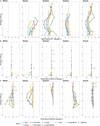
Table 3. Long-term average of the NDVI, SWA, and SCA for the period between December 2002 and November 2021 at seasonal and annual temporal scale. SD: Standard deviation.

Basin		NDVI		SWA [km^2]		SCA [km^2]
	Season	Mean	SD	Mean	SD	Mean	SD
Lower Ural	Winter	0.037	0.038	8,651	2,959	–	–
	Spring	0.234	0.053	14,234	4,163	–	–
	Summer	0.313	0.039	8,993	3,092	–	–
	Autumn	0.233	0.041	9,421	2,454	–	–
	Annual	0.205	0.043	10,325	3,167	–	–
Uzboy	Winter	0.127	0.033	30,086	1,276	26,826	9,441
	Spring	0.192	0.028	30,753	573	6,594	3,758
	Summer	0.151	0.028	30,341	356	53	46
	Autumn	0.140	0.010	30,223	396	2,485	2,172
	Annual	0.152	0.021	30,353	650	8,990	3,854
Syr Darya	Winter	0.024	0.028	10,198	2,723	164,768	11,484
	Spring	0.213	0.039	21,044	3,601	101,138	18,036
	Summer	0.278	0.023	19,089	1,532	18,030	5,234
	Autumn	0.187	0.025	18,098	1,674	61,695	20,039
	Annual	0.175	0.029	17,107	2,382	86,408	13,698
Amu Darya	Winter	0.107	0.036	13,290	6,072	234,934	22,084
	Spring	0.208	0.025	18,975	7,144	167,376	19,152
	Summer	0.201	0.012	16,974	7,501	51,835	11,991
	Autumn	0.162	0.012	16,143	6,705	89,183	27,477
	Annual	0.169	0.021	16,345	6,855	135,832	20,176
Irtysh	Winter	−0.001	0.011	3,079	2,266	107,503	1,561
	Spring	0.179	0.052	23,369	6,203	82,092	9,552
	Summer	0.507	0.037	28,354	2,284	10,133	4,902
	Autumn	0.251	0.054	28,968	3,899	61,720	13,788
	Annual	0.234	0.038	20,943	3,663	65,362	7,450
Lake Balkash	Winter	0.010	0.021	13,684	3,904	112,583	5,220
	Spring	0.210	0.041	29,501	4,608	65,268	12,620
	Summer	0.337	0.026	36,139	319	13,060	3,133
	Autumn	0.199	0.031	36,344	1,200	49,476	13,485
	Annual	0.189	0.030	28,917	2,508	60,097	8,614
Gobi Interior	Winter	0.008	0.017	1,992	853	37,182	3,424
	Spring	0.199	0.047	5,186	1,132	19,053	4,231
	Summer	0.414	0.032	7,491	268	3,299	705
	Autumn	0.223	0.038	7,338	347	15,670	4,754
	Annual	0.211	0.034	5,502	650	18,801	3,279

At basin scale, elevation-dependent trends were calculated for the NDVI, SWA, and SCA (Figure 4). The NDVI showed significant positive trends at altitudes above 1,500 m in the Lake Balkash basin during the spring season. However, in summer the trends in NDVI were significantly negative in the Lake Balkash basin for the same altitudes. In the Irtysh basin, the NDVI trends were significantly positive at altitudes above 2,000 m. In summer, significant positive trends were also detected in the Amu Darya basin at high altitudes (Figure 4(a)). Next, SWA showed the highest magnitude in significant trends in low altitudes (Figure 4(b)). As in Table 2, the magnitude in SWA trends was highest in the Amu Darya basin. Considering SCA, the elevation-dependent trends resulted in significant negative trends in the winter season with particularly high magnitudes in the Amu Darya, Uzboy, and Syr Darya basins (Figure 4(c)). At altitudes above 1,500 m, the trends were generally significantly negative in the Syr Darya and Lake Balkash basins except during autumn. For example, in the spring season significant negative trends were detected in the Syr Darya and Lake Balkash basins with comparatively high magnitudes at altitudes between 1,5000 and 3,000 m. In the summer season, SCA appeared to decrease significantly at altitudes above 3,500 m in the Lake Balkash basin.

3.3. Trends at national scale

Further trend analyses were performed at national scale for the land surface variables and additional vegetation classes (Table 4). In Kazakhstan, significant trends were detected seasonally for rainfed and irrigated croplands. During summer, the NDVI for both vegetation classes showed significant negative trends. SWA trends were significant negative for all seasons, being particularly pronounced during the summer. Likewise, SWA showed significant negative trends throughout all seasons in Turkmenistan. However, the magnitude of trends was found to be low. In comparison to SWA, significant positive trends were detected for forest areas in Turkmenistan. In Uzbekistan, SCA showed a significant negative trend for the winter season with a considerable magnitude. SWA in Uzbekistan indicated a significant positive trend in winter and negative trends in the other seasons. Significant negative trends were also retrieved for Tajikistan and Kyrgyzstan for SCA in the winter and spring season. In the spring season, all vegetation classes resulted in significant positive NDVI trends in Kyrgyzstan.

Table 4. Annual and seasonal trends at national scale for the NDVI, SWA, and SCA. Additionally, trends were calculated for vegetation classes using the ESA CCI land cover data and NDVI. All trend values are computed at decadal scale. Bold values represent statistically significant trends (p-value < 0.05). Trends for SWA and SCA are indicated in 1,000 km². NDVI and vegetation classes are in NDVI unit.

Country	Class	Winter	Spring	Summer	Autumn	Annual
Kazakhstan	NDVI	–	0.007	−0.009	−0.009	−0.009
	Forest	–	0.018	0.005	−0.012	0.005
	Grassland	–	0.011	−0.007	−0.008	−0.007
	Cropland	–	0.000	−0.018	−0.011	−0.011
	Irrigation	–	0.013	−0.014	−0.014	−0.014
	SWA	−0.970	−5.261	−7.003	−6.641	−5.951
	SCA	−46.427	−8.943	−0.795	17.695	−4.869
Turkmenistan	NDVI	–	0.001	0.001	–	0.001
	Forest	0.010	0.012	0.017	0.008	0.011
	Grassland	−0.001	−0.001	0.001	−0.001	−0.001
	Cropland	−0.007	0.008	0.007	–	0.007
	Irrigation	0.011	0.005	0.000	−0.002	0.003
	SWA	−0.084	−0.223	−0.217	−0.252	−0.220
	SCA	−2.218	−0.100	–	0.028	−0.100
Uzbekistan	NDVI	–	−0.003	−0.001	−0.003	−0.003
	Forest	–	0.006	−0.005	−0.008	−0.005
	Grassland	–	−0.001	−0.006	−0.002	−0.002
	Cropland	–	−0.004	−0.006	−0.001	−0.004
	Irrigation	0.013	0.009	0.007	−0.003	0.008
	SWA	2.627	−4.161	−1.365	−1.676	−1.520
	SCA	−31.529	0.430	−0.020	0.601	0.205
Tajikistan	NDVI	–	0.012	−0.001	–	0.005
	Forest	–	0.024	0.003	0.001	0.003
	Grassland	–	0.018	0.000	−0.002	0.000
	Cropland	–	0.008	−0.007	−0.001	−0.001
	Irrigation	–	0.032	0.011	−0.005	0.011
	SWA	0.039	0.016	0.014	0.037	0.026
	SCA	−4.239	−2.685	−1.383	0.260	−2.034
Kyrgyzstan	NDVI	–	0.031	−0.004	–	0.013
	Forest	–	0.042	−0.005	−0.011	−0.005
	Grassland	–	0.032	−0.003	−0.008	−0.003
	Cropland	–	0.032	−0.003	−0.009	−0.003
	Irrigation	–	0.036	−0.002	−0.013	−0.002
	SWA	−0.002	0.003	−0.037	−0.041	−0.020
	SCA	−5.792	−8.301	−1.344	2.767	−3.568

3.4. Trends at grid scale

Figure 5 provides insights on the spatial patterns of the seasonal trends of the NDVI, SWA, and SCA. In terms of the spatial distribution of trends, NDVI showed a two-fold pattern with respect to the direction of trends. This pattern is particularly pronounced in the summer season, where significant negative trends are dominant in the Northwest and significant positive trends in the Northeast of the study area (Figure 5(a)). In total, the NDVI demonstrated significant positive and negative trends for 15.4 and 30.5% of the grids, respectively (Table 5). In almost all seasons the share of significant negative trends outweighs the positive trends, except for the spring season, where significant positive and negative trends amounted to 14.1 and 4.8% of the grids, respectively (Table 5). Throughout all seasons, significant positive trends are pronounced in the Northeast of Kazakhstan and in areas south of the Aral Sea. Considering trends in SWA, Figure 5(b) shows that significant negative trends are dominant throughout the study region. For example, during summer and autumn the percentage of significant negative trends amounted to 33.1 and 37.8%, respectively (Table 5). In comparison, the significant positive trends were at 22.5 and 15.2%, respectively (Table 5). In terms of the spatial distribution, it appears that the areas close to the Amu Darya and Syr Darya were particularly affected by the decline in SWA (Figure 5(b)). With respect to SCA in mountainous regions of CA, the results indicated a significant decline for 23.0% of the grids in winter (Table 5), being most prominent in the Pamir-Alay and northern Tian Shan mountains. During spring and summer, the share of significant negative trends considerably outweighed the significant positive trends as well. Only in autumn, for 11.6% of the grids significant positive SCA trends could be detected (Table 5). In terms of the spatial distribution of the trends, Figure 5c shows that particularly the northern Tian Shan mountains are impacted by the declining SCA. In contrast, high elevation zones in the Northeast, i.e. in the Dzungarian Alatau mountains, SCA appears to have increased in autumn.

Figure 5. Annual and seasonal trends for the (a) NDVI, (b) SWA, and (c) SCA between December 2002 and November 2021. The meteorological seasons winter, spring, summer, and autumn as well as the annual scale were considered for the trend metrics. Grids outside the 95% confidence level are colored in gray (not significant).

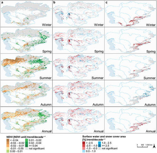
Table 5. Percentage of significant positive and negative trends at grid scale for the entire study area. The significant trends (sig.) include grids with a p-value < 0.5. The percentages for all trends and tendencies sum up to 100% and include non-significant trend values as well.

		Winter		Spring		Summer		Autumn		Annual
Variable	Significance	+	–	+	–	+	–	+	–	+	–
NDVI	sig.	9.4	15.9	14.1	4.8	15.4	30.5	4.7	19.1	15.7	27.4
	all	43.0	57.0	63.3	36.7	41.1	58.9	32.3	67.7	42.1	57.9
SWA	sig.	14.5	10.5	15.5	26.5	22.5	33.1	15.2	37.8	21.2	41.2
	all	61.7	38.3	45.7	54.3	45.4	54.6	35.0	65.0	38.5	61.5
SCA	sig.	1.3	23.0	0.2	15.6	0.7	5.7	11.6	1.4	1.9	17.3
	all	31.5	68.5	21.1	78.9	36.4	63.6	70.1	29.9	28.8	71.2

3.5. Direct drivers of the land surface variables

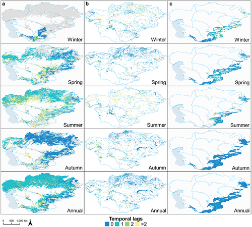
Figure 6 highlights the driving variables that have the largest effect size at grid scale on the NDVI, SWA, and SCA. Considering the NDVI, Figure 6(a) suggests that temperature was the most influential controlling factor during winter and autumn with a share of 75.9 and 45.2% among all grids having a significant link, respectively. The detected coupling with temperature was largely positive. During spring and summer, soil moisture was the variable with the largest influence on the vegetation with a share of 27.3 and 47.0% of all grids, respectively. Also, the coupling with soil moisture and vegetation was positive for almost all grids having this link. However, during spring, temperature was found to have a large effect size in the Northeast of CA. Here, it is striking that temperature appeared to have an immediate effect (temporal lag of 0) on the vegetation during most of the seasons (Figure 7(a)). In comparison, soil moisture was found to impact vegetation with a temporal lag of 1 at biweekly intervals during the spring and summer season. Moreover, areas where irrigated agriculture is predominant, e.g. along the Syr Darya and Amu Darya river, soil moisture was found to be the most important driver throughout all seasons. Also, in the summer season, vapor pressure deficit was coupled negatively with the NDVI in northern CA. This negative link occurred in 14.2% of the grids having significant links. At higher elevations, SCA was negatively coupled with NDVI particularly in spring and autumn (Figure 6(a)). The identified links with SWA are displayed in Figure 6(b). Here, river discharge and temperature were mostly detected as drivers having the largest influence on SWA with the temporal lags of 0–2 being prominent (Figure 7(b)). Both drivers were positively coupled with SWA. In comparison, SCA was also identified as driver in mountainous areas throughout the seasons, except in summer. Here, the coupling was negative, mostly at biweekly lags 0–1. Considering the drivers of SCA, temperature was identified to have the largest impact at grid scale (Figure 6(c)). In spring and autumn, temperature was negatively coupled with SCA for 58.9 and 85.1% of the grids having a significant link. This link was prominent at lags 0–1 (Figure 7(c)). Precipitation was found to have the largest influence during winter (19.1%) and spring (9.9%), being dominant mostly in the Tian Shan mountains. Here, this link was mostly found at lag 1 (Figure 7(c)).

Figure 6. This map shows the drivers that have the maximum effect size at grid and seasonal as well as annual scale on the land surface variables (a) NDVI, (b) SWA, and (c) SCA. The calculation of the causal networks was performed for the meteorological seasons winter, spring summer, and autumn. For the NDVI, additional phenological thresholds were considered as indicated in section 2.3.2. The feature space included the variables precipitation (P), surface solar radiation downward (DSR), temperature (T), vapor pressure deficit (VPD), soil moisture (SM), river discharge (Q), SWA, and SCA. Grids that are colored gray have no significant causal link. The land surface variables were analyzed with a different set of drivers: (a) NDVI: P, DSR, T, VPD, SM, SWA; (b) SWA: P, DSR, T, Q, SCA; (c) SCA: P, DSR, T.

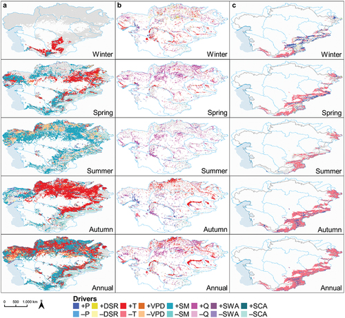
Figure 7. This map shows the detected temporal lags with the largest effect size per grid with respect to the identified causal links in Figure 5.

3.6. Analysis of interdependencies

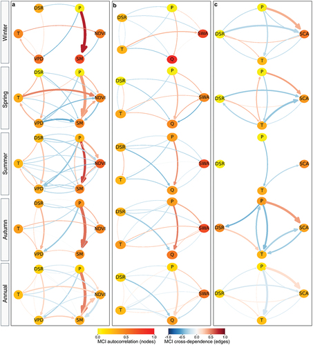
Besides the direct influences on the land surface variables, the analysis of causal graphs provides further insights into the direct and indirect relations among the investigated variables. In this regard, Figure 8 presents three separate feature spaces, each being representative for one of the land surface variable NDVI, SWA, and SCA. Here, the identified causal links were visualized as causal graphs (Figure 8). The calculation of the causal graphs considered a maximum number of 171 subbasins. For each subbasin, the causal graphs were calculated separately considering temporal lags between 1 and 3 biweekly steps. Afterwards, the graphs were aggregated for the investigated region at seasonal scale. Figure 8a shows the graphs for the NDVI. Dominant links throughout the seasons include direct connections between the variables precipitation and soil moisture, soil moisture and NDVI as well as temperature and NDVI. As an example, besides, the direct influence of precipitation on NDVI in the spring and summer season, there is also an indirect path between precipitation and NDVI through soil moisture (Figure 8a; spring, summer). Also, it can be seen that the NDVI is negatively coupled to soil moisture in these seasons. Temperature is generally positively coupled to the NDVI, except during summer. In summer, vapor pressure deficit is negatively coupled to the NDVI. Figure 8b illustrates the detected causal links for the feature space including SWA. Here, precipitation shows a direct and positive impact on SWA in all seasons, except summer. This link was found to be present indirectly through river discharge as well. In summer, both river discharge and precipitation showed a negative influence on SWA. Furthermore, Figure 8c presents the significant links being identified within the feature space for SCA. For summer, precipitation showed a positive influence on SCA. In comparison, as already outlined in the grid scale analysis, temperature largely shows a negative influence on SCA in all seasons. Solar radiation was found to negatively influence SCA directly during winter and spring as well as indirectly in autumn through temperature. For individual seasons, there was also a negative link from SCA toward temperature.

Figure 8. The calculated causal graphs show the interdependencies of the used time series, including (a) the NDVI, (b) SWA, and (c) SCA. Three temporal lags were considered for the calculation of the causal graphs. A low frequency of a causal link at subbasin scale is depicted by a thin edge and vice versa. Besides the land surface variables, following time series were considered: precipitation (P), surface solar radiation downward (DSR), temperature (T), vapor pressure deficit (VPD), soil moisture (SM), river discharge (Q).

4. Discussion

4.1. Trends and controlling factors of land surface variables

4.1.1. Vegetation

This study analyzed the trends and drivers of land surface variables at different spatial and temporal scales for CA using multivariate time series. Available studies on vegetation trends over CA pointed toward comparable trends in terms of their direction as well as spatial patterns as found in this study (Y. Li et al. 2021; Luo et al. 2020; Xu, Wang, and Zhang 2016; Yuan et al. 2017; G. Zhang et al. 2018; W. Zhang et al. 2021; Zheng et al. 2021). For example, Zheng et al. (2021) reported significant positive trends for pastures in the Tian Shan mountains. Yet, in areas close to the Issyk-Kul Lake they identified significant negative trends in the NDVI as well. This aligns with findings of this investigation. Also, Zheng et al. (2021) presented significant positive trends for high elevation zones (>4,000 m) in the Tian Shan mountains. Their observation matches our findings of significant positive NDVI trends for high elevation zones of the Lake Balkash basin in the spring season (Figure 5a). However, in summer and autumn, the identified trends within our study were mostly significantly negative. This might be caused by the slightly differing study period (2000–2020). In contrast to Zheng et al. (2021), Liu et al. (2021) found a browning trend of vegetation between 1998 and 2015 in high elevation zones. The significant negative trends were particularly pronounced in the Tian Shan mountains. Likewise, Li et al. (2021) reported a general browning trend for vegetation in the Tian Shan mountains since 1998. Furthermore, significant negative trends were also found for areas in the North and Northwest of CA for the period 2003 to 2015 by Zhang et al. (2021). Here, the direction and the spatial pattern of trends were similar to this study. Further available studies for the period until 2015 reported comparable significant negative trends for vegetated areas over CA (Luo et al. 2020; Xu, Wang, and Zhang 2016; Yuan et al. 2017; G. Zhang et al. 2018). For instance, Zhang et al. (2018) focused on grasslands and identified a considerable grassland degradation and expansion of desertification in northern Kazakhstan. This finding might align with the reported significant negative trends of this study. Additionally, the observed peaks in the annual NDVI time series during 2008 in the Amu Darya and Uzboy basins (Figure 3) might be explained with the occurrence of severe drought events in this region (Patrick 2017; Yoo et al. 2022).

With respect to the drivers of vegetation greenness, the findings of this study showed a large seasonal dependency on temperature and water availability, with temperature being prominent in spring and autumn and soil moisture in spring and summer. The positive coupling with temperature is most likely to be explained with temperature acting as a limiting factor in cold periods in this region. The positive influence of soil moisture during the start of the season and in summer is most likely linked to the water needs of growing vegetation. During summer there are large areas in northern CA showing a negative coupling with vapor pressure deficit (Figure 6a). At the same time, these vegetated areas mostly indicated a significant negative trend during summer (Figure 5). This could be an indication toward increasing temperature and vapor pressure deficit having a negative influence on vegetation health. In this regard, Hao et al. (2022) pointed toward the importance of water availability and vapor pressure deficit as potential limiting factors of vegetation growth in CA. Zhang et al. (2021) emphasized the importance of soil moisture and vapor pressure deficit on vegetation in CA during 2003–2015 as well. The findings of Zhang et al. (2021) include an earlier start as well as end of the growing season. The authors state that an earlier start of the season might lead to a higher soil moisture deficit in the late growing season and hence cause drought stress on vegetation. In this regard, the findings of this study support this shift in the vegetation phenology with largely significant positive trends as well as positive tendencies (including non-significant) in the spring season accounting for 14.1 and 63.3% of the grids, respectively (Figure 5a, Table 5). In comparison, during autumn this pattern was found to be the opposite with largely significant negative trends and negative tendencies (including non-significant) amounting to 19.1 and 67.7% of the grids (Figure 5a, Table 5).

Furthermore, agricultural fields, in particular irrigated fields, were found to be an important driver of greening vegetation trends in the southern basins of the Tibetan Plateau (Chen et al. 2019; Uereyen et al. 2022). However, the findings of this study underline that the role of agricultural land use with respect to greening vegetation in CA is not as important as in other regions, where intensification and extensification of agricultural land use was identified as an important driver of the greening (Chen et al. 2019). The reason for this is most likely the limited availability of freshwater over the mostly arid regions of CA.

Considering the influence of SCA on vegetation, previous investigations reported an advancing start of the growing season, e.g. in areas close to the Issyk-Kul Lake (L. Wu et al. 2021; Zheng et al. 2021). In this context, we found that in the spring season for 27.6% of the grids, where SCA has a significant negative trend, NDVI resulted in a significant positive trend. With phenological shifts in SCA, the phenology of vegetation in mountainous regions might further change in future, being also implied by the strong negative coupling of the NDVI and SCA during spring and autumn (Figure 6a) as well as in significant positive trends of vegetation at high elevations of the Lake Balkash basin (Figure 4a). Here, it can be added that temperature and precipitation might act as an indirect driver of changes in SCA and the NDVI. For example, temperature indicated a significant positive trend during summer and positive tendencies during winter and spring in the Lake Balkash basin (Table 2). Increasing temperatures in higher elevations were also presented by Zheng et al. (2021).

4.1.2. Surface water area

Significant trends for SWA were mostly negative at grid, basin, and national scale. Here, it is noteworthy that the river discharge in the Amu Darya, Syr Darya, and Lake Balkash basins mainly depends on meltwater from glaciers and snow, with the share being largest in the Amu Darya (Kraaijenbrink et al. 2021; Qin et al. 2020). In this regard, Zhang et al. (2022) identified an increase in the area of glacial lakes in the Tian Shan mountains, being related to a warming climate and retreat of glaciers. Liu et al. (2019) analyzed changes in lake area for 17 lakes in CA. For lakes situated in plains they found significant decreasing trends in their area and for lakes at higher elevations significant positive trends. In comparison, the magnitude of significant negative trends found in our study was particularly high in Uzbekistan and Kazakhstan (Table 4). Likewise, a decline in permanent SWA and terrestrial water storage in CA as well as in the Aral Sea region was also presented by Huang et al. (2021b) and Yang et al. (2020), respectively. In addition, Che et al. (2019) analyzed seasonal changes in SWA in CA between 2000 and 2015 using Landsat imagery. Their conclusion included a significant decrease in SWA as well.

The driver analysis of this study, considering only environmental drivers, identified river discharge and temperature as the most important variables describing seasonal SWA dynamics (Figure 6b). Temperature was particularly important during winter and autumn. This positive coupling of temperature and SWA, which was also identified in the causal graphs (Figure 8b) might be explained by freezing SWA in cold periods. Further studies investigated potential human impacts on SWA in CA. Huang et al. (2021b) stated that human activities might be the primary cause for declines in SWA due to population growth, dam constructions, and water use for irrigation purposes. Similarly, Yang et al. (2020) reported that the reductions of SWA in the Aral Sea are primarily linked to human activities and that this decrease could not be compensated by an increase in precipitation as well as meltwater availability from glaciers and snow. In this regard, Rodell et al. (2018) also pointed toward a decrease in glaciers in the Tian Shan mountains being linked to global warming. In addition, the authors emphasize groundwater depletion in this region being also caused by irrigation activities. Despite the identified major significant decreases in SWA at all investigated spatial scales (e.g. Figure 5b) as well as decreasing river discharge, the number of people depending on freshwater from the rivers Amu Darya and Syr Darya is still increasing (Viviroli et al. 2020).

4.1.3. Snow cover area

Nearly all significant trends at basin and seasonal scale for SCA had a negative direction being particularly pronounced in the Amu Darya, Syr Darya, and Lake Balkash basins (Table 2). The findings with regard to elevation-dependent trends in this study are consistent with trends identified by Li et al. (2020a). Likewise, further studies also found increasing snow line elevation in the Tian Shan mountains (Deng et al. 2021; Tang et al. 2020). Matching significant negative trends were also shown for the Syr Darya basin covering the period 2002–2017 by Ackroyd et al. (2021). In addition, the results of Notarnicola (2020b) indicated comparable trends for SCA in the investigated basins between 2000–2018. Due to the larger temporal coverage of this study, it can be noted that the significant negative trends in the Syr Darya, Amu Darya, and Lake Balkash basins appear to persist and amplify. In comparison, during autumn significant positive trends were revealed in the eastern parts of CA. For these areas, non-significant positive tendencies were reported at annual scale by Notarnicola (2020b). The differences between the results might be caused by the different length of the investigated period.

Considering the controlling variables of SCA at grid scale, it was found that precipitation had the highest influence during winter. The positive coupling of SCA and precipitation might be explained by the Karakoram Anomaly, which leads to comparatively high precipitation amounts over the western parts of the Tibetan Plateau (Miles et al. 2021). In comparison, temperature was found to be negatively coupled with SCA and was the dominant driver during the other seasons (Figure 6c). Furthermore, the analysis of the causal graphs revealed that besides the negative influence of temperature on SCA, SCA was also found to negatively influence temperature in autumn (Figure 8c). This coupling might be explained by the onset of emerging snowfall resulting in an increase in SCA, thus influencing the snow-albedo feedback. In fact, warming temperatures over high altitudes of CA were identified e.g. by Kraaijenbrink et al. (2021). In this regard, temperature was also found to be the main driver of changes in the cryosphere of CA (Barandun et al. 2020; Z. Li, Chen, et al. 2020). Besides changes in SCA, projections show that glaciers in this region might face considerable reductions in their volume. In particular, estimations revealed declines in glacier volume of approximately 31% for the Tian Shan and 17% for the Pamir (Miles et al. 2021). Since snow and glacier meltwater contribute largely to the streamflow in the downstream basins of the mountains of CA, changes in the seasonality and the amount of meltwater could have severe implications on the water availability for the population and water-dependent sectors.

4.2. Future implications

The land surface dynamics in CA will likely be primarily shaped by the amplified climate warming as well as future changes in spatial and temporal patterns of precipitation. Future projections showed that the annual amount of precipitation in CA might increase, due to an intensification in extreme events (Yao et al. 2021). Similarly, Luo et al. (2018) reported an average increase of precipitation over CA, but with spatiotemporal differences and particularly a decrease in Central and South CA in the summer season. So far, increases in temperature were most conspicuous over northern CA as well as at higher altitudes (Luo et al. 2018). Furthermore, temperature increases in large parts of CA appear to be higher than the global average (J. Huang et al. 2017). Also, projections showed an increase in the frequency of heatwaves in CA (Fan et al. 2022). Considering the Amu Darya basin, Salehie et al. (2022) reported that in future, warming temperatures will occur particularly in the source region of the river basin. In this regard, decreases in glacier volumes and SCA caused by a changing climate will likely have impacts on the vulnerability of river basins being dependent on meltwater from their source regions and increase the uncertainties of water resources management in CA (Barandun et al. 2020; Q. Zhang et al. 2022).

Furthermore, it was noted that the Amu Darya and Syr Darya river basins are highly relying on meltwater from the source regions (Qin et al. 2020). At the same time, these basins inherit most of the irrigated agricultural areas in CA. Besides the agricultural sector, water availability has a great importance with respect to further domestic needs, including the population and hydropower generation (Barandun et al. 2020; Reyer et al. 2015). Considering vegetated areas in the Amu Darya and Syr Darya basins, significant negative NDVI trends could be observed regionally over the last two decades (Figure 5a). Further trend analyses at basin scale indicated no clear trend for vegetation in both basins, but in the Lake Balkash basin significant positive trends were obtained for the spring and summer season (Figure 4a). Particularly for the irrigated areas in Southern and Central parts of CA, including Uzbekistan and Kazakhstan, water demand is high during summer. With changing meltwater contributions to the river discharge as well as shifts in the peak discharge, projected increases in extreme precipitation events, and increases in the frequency of drought events, vegetated areas, in particular agricultural land use, will likely be negatively impacted in the future (Z. Li, Fang, et al. 2020; Ren et al. 2022). In this context, it was identified that by mid-century there is a high risk, that the water demand in summer might not be met anymore by meltwater in the Amu Darya and Syr Darya river basins (Mankin et al. 2015). Xu et al. (2016) found out that past drought events have contributed to the negative NDVI trends in CA, particularly in the Northern areas of Kazakhstan. In regards of droughts and changing precipitation patterns, vegetated areas, particularly rainfed agriculture being located in the northern parts of Kazakhstan might be particularly vulnerable (Reyer et al. 2015). To enable the development of adaptation strategies and inform stakeholders, the quantification and analysis of recent land surface processes remains an important task. The findings of this study could contribute to a better understanding of land surface dynamics in this region and might support the regional development of adaptation strategies in the context of a warming climate.

4.3. Limitations of this study

The investigated trends and drivers of the land surface variables depend on several factors, including data accuracy and spatial as well as temporal resolution of the data. The used satellite image-based time series were generated by means of MODIS data. To overcome gaps and enable the creation of a dense and consistent time series, both MODIS sensors were used. Yet, the MODIS data only covers a period of two decades limiting long-term analysis of trends in the land surface variables. Furthermore, the spatial resolution of the MODIS and reanalysis data might be too coarse to analyze the interdependencies of the variables, e.g. in topographically complex areas. In this regard, the availability of meteorological time series with a higher spatial resolution and a regional focus on CA might enhance the analyses, e.g. regarding the elevation-dependent zones. Furthermore, the lack of gridded time series being representative for anthropogenic influence hampers the quantification of the corresponding impacts on the land surface. Yet, with the trend analyses at national scale for different vegetation classes, we aimed at providing insights into potential human influences on vegetated areas.

5. Conclusions

This study investigated land surface dynamics in Central Asia (CA) over the last two decades using remote sensing-based time series for the land surface variables normalized difference vegetation index (NDVI), surface water area (SWA), and snow cover area (SCA). First, we calculated trends at seasonal and annual scale to analyze changes for the investigated variables. The trend analysis was conducted at different spatial scales, including spatial grids, hydrological basins, national borders, and elevation zones. The main findings of the trend analysis are:

• During summer, significant NDVI trends were mostly negative in the Northwest and positive in the Northeast of CA. The share of significant negative trends for the NDVI were higher than the positive trends in summer and autumn seasons, as well as at annual temporal scale. Rainfed and irrigated croplands resulted in significant negative trends in Kazakhstan with −0.018 and −0.014 NDVI decade⁻¹, respectively. The analysis indicated that irrigated agriculture was not contributing to positive trends in this region.

• SWA mostly indicated significant negative trends across all temporal and spatial scales. Particularly in the Amu Darya river basin, SWA appeared to decline by 14,173 km² decade⁻¹ during spring. At grid scale, the significant negative trends in SWA were most prominent in the Aral Sea region.

• SCA showed significant negative trends across all temporal scales, except for autumn, where positive trends were observed in the Altai and Dzungarian Alatau mountains. Significant negative trends were prominent in the Tian Shan and Pamir mountains during winter and spring. In the Amu Darya and Syr Darya basin, SCA was found to decline by 8,849 and 3,987 km² decade⁻¹ during winter, respectively. SCA in the Lake Balkash basin showed a negative trend of 6,790 km² decade^{− 1} during spring.

Additional time series were used to evaluate controlling factors of the investigated land surface variables. To the best of our knowledge, the used causal discovery algorithm was not applied for the analysis of seasonal drivers in CA so far. For the NDVI, water availability was found to be the dominant driver in summer for 47.0% of all grids. During spring and autumn, temperature had a large influence on vegetation. SWA was found to be positively linked to temperature during autumn and winter. River discharge was the variable having the largest influence at grid scale and precipitation was found to be important regionally. Moreover, SCA was mostly negatively influenced by temperature during spring and autumn for 58.9 and 85.1% of all grids, respectively. During winter, precipitation was found to positively control SCA, particularly in the Tian Shan mountains.

For available climate change scenarios, CA is found to face a warming above the global average making this region a climate change hotspot. It is emphasized that the Amu Darya and Syr Darya river basins highly rely on meltwater from the source regions, particularly in the summer season when agricultural activities are at its peak. Hence, any shifts in the availability of meltwater from snow and glaciers, peak discharge or precipitation and temperature patterns will likely negatively influence vegetated areas, particularly irrigated agriculture. In addition, a higher frequency of droughts in the future might negatively impact rainfed croplands in northern areas of CA as well. In this regard, this study aimed at assessing and improving the understanding of the recent evolution of the land surface in CA using remote sensing time series.

Acknowledgment

We acknowledge funding from the GIZ (Gesellschaft für Internationale Zusammenarbeit) within the framework of the project ”ECO-ARAL” (Ecologically Oriented Development in the Aral Sea Region).

Disclosure statement

No potential conflict of interest was reported by the author(s).

Data availability statement

The DLR Global WaterPack and DLR Global SnowPack are available for download at the EOC Geoservice (https://geoservice.dlr.de/web/).

References

- Ackroyd, C., S. M. Skiles, K. Rittger, and J. Meyer. 2021. “Trends in Snow Cover Duration Across River Basins in High Mountain Asia from Daily Gap-Filled MODIS Fractional Snow Covered Area.” Frontiers in Earth Science 9:713145. https://doi.org/10.3389/feart.2021.713145.
- Barandun, M., J. Fiddes, M. Scherler, T. Mathys, T. Saks, D. Petrakov, and M. Hoelzle. 2020. “The State and Future of the Cryosphere in Central Asia.” Water Security 11:100072. https://doi.org/10.1016/j.wasec.2020.100072.
- Barkhordarian, A., S. S. Saatchi, A. Behrangi, P. C. Loikith, and C. R. Mechoso. 2019. “A Recent Systematic Increase in Vapor Pressure Deficit Over Tropical South America.” Scientific Reports 9 (1): 15331. https://doi.org/10.1038/s41598-019-51857-8.
- Beck, H. E., N. E. Zimmermann, T. R. McVicar, N. Vergopolan, A. Berg, and E. F. Wood. 2018. “Present and Future Köppen-Geiger Climate Classification Maps at 1-Km Resolution.” Scientific Data 5 (1): 180214. https://doi.org/10.1038/sdata.2018.214.
- Bhattacharya, A., T. Bolch, K. Mukherjee, O. King, B. Menounos, V. Kapitsa, N. Neckel, W. Yang, and T. Yao. 2021. “High Mountain Asian Glacier Response to Climate Revealed by Multi-Temporal Satellite Observations Since the 1960s.” Nature Communications 12 (4133): https://doi.org/10.1038/s41467-021-24180-y.
- Che, X., M. Feng, J. Sexton, S. Channan, Q. Sun, Q. Ying, J. Liu, and Y. Wang. 2019. “Landsat-Based Estimation of Seasonal Water Cover and Change in Arid and Semi-Arid Central Asia (2000–2015).” Remote Sensing 11 (11): 1323. https://doi.org/10.3390/rs11111323.
- Chen, C., T. Park, X. Wang, S. Piao, B. Xu, R. K. Chaturvedi, R. Fuchs, et al. 2019. “China and India Lead in Greening of the World Through Land-Use Management.” Nature Sustainability 2 (2): 122–23. https://doi.org/10.1038/s41893-019-0220-7.
- Collaud Coen, M., E. Andrews, A. Bigi, G. Martucci, G. Romanens, F. P. A. Vogt, and L. Vuilleumier. 2020. “Effects of the Prewhitening Method, the Time Granularity, and the Time Segmentation on the Mann–Kendall Trend Detection and the Associated Sen’s Slope.” Atmospheric Measurement Techniques 13:6945–6964. https://doi.org/10.5194/amt-13-6945-2020. 12
- Deng, G., Z. Tang, G. Hu, J. Wang, G. Sang, and J. Li. 2021. “Spatiotemporal Dynamics of Snowline Altitude and Their Responses to Climate Change in the Tienshan Mountains, Central Asia, During 2001–2019.” Sustainability 13 (7): 3992. https://doi.org/10.3390/su13073992.
- Dietz, A. J., C. Kuenzer, and S. Dech. 2015. “Global SnowPack: A New Set of Snow Cover Parameters for Studying Status and Dynamics of the Planetary Snow Cover Extent.” Remote Sensing Letters 6 (11): 844–853. https://doi.org/10.1080/2150704X.2015.1084551.
- Ding, C., W. Huang, M. Liu, and S. Zhao. 2022. “Change in the Elevational Pattern of Vegetation Greenup Date Across the Tianshan Mountains in Central Asia During 2001–2020.” Ecological Indicators 136:108684. https://doi.org/10.1016/j.ecolind.2022.108684.
- European Space Agency. 2017. Land Cover CCI Product User Guide Version 2. Tech. Rep. In.
- European Space Agency, & Sinergise. 2021. Copernicus Global Digital Elevation Model. Distributed by OpenTopography. Accessed January 1, 2024. https://doi.org/10.5069/G9028PQB.
- Fan, L.-J., Z.-W. Yan, D. Chen, and Z. Li. 2022. “Assessment of Central Asian Heat Extremes by Statistical Downscaling: Validation and Future Projection for 2015‒2100.” Advances in Climate Change Research 13 (1): 14–27. https://doi.org/10.1016/j.accre.2021.09.007.
- Granger, C. W. J. 1969. “Investigating Causal Relations by Econometric Models and Cross-Spectral Methods.” Econometrica 37 (3): 424. https://doi.org/10.2307/1912791.
- Gulakhmadov, A., R. Davlyatov, Z. Kobuliev, and X. Chen. 2021. “Elevation Dependency of Climatic Variables Trends in the Last Decades in the Snow-Fed and Glacier-Fed Vakhsh River Basin, Central Asia.” Water Resources 48 (6): 914–924. https://doi.org/10.1134/s0097807821060075.
- Hao, H., Y. Chen, J. Xu, Z. Li, Y. Li, and P. M. Kayumba. 2022. “Water Deficit May Cause Vegetation Browning in Central Asia.” Remote Sensing 14 (11): 2574. https://doi.org/10.3390/rs14112574.
- Harrigan, S., E. Zsoter, L. Alfieri, C. Prudhomme, P. Salamon, F. Wetterhall, C. Barnard, H. Cloke, and F. Pappenberger. 2020. “GloFAS-ERA5 Operational Global River Discharge Reanalysis 1979–Present.” Earth System Science Data 12 (3): 2043–2060. https://doi.org/10.5194/essd-12-2043-2020.
- Huang, W., W. Duan, and Y. Chen. 2021. “Rapidly Declining Surface and Terrestrial Water Resources in Central Asia Driven by Socio-Economic and Climatic Changes.” Science of the Total Environment 784:147193. https://doi.org/10.1016/j.scitotenv.2021.147193.
- Huang, F., T. Feng, Z. Guo, and L. Li. 2021. “Impact of Winter Snowfall on Vegetation Greenness in Central Asia.” Remote Sensing 13 (21): 4205. https://doi.org/10.3390/rs13214205.
- Huang, J., H. Yu, A. Dai, Y. Wei, and L. Kang. 2017. “Drylands Face Potential Threat Under 2 °C Global Warming Target.” Nature Climate Change 7 (6): 417–422. https://doi.org/10.1038/nclimate3275.
- Hu, Q., and Z. Han. 2022. “Northward Expansion of Desert Climate in Central Asia in Recent Decades.” Geophysical Research Letters 49 (11). https://doi.org/10.1029/2022gl098895.
- Hu, Z., Q. Hu, C. Zhang, X. Chen, and Q. Li. 2016. “Evaluation of Reanalysis, Spatially Interpolated and Satellite Remotely Sensed Precipitation Data Sets in Central Asia.” Journal of Geophysical Research: Atmospheres 121 (10): 5648–5663. https://doi.org/10.1002/2016jd024781.
- IPCC. 2018. Global Warming of 1.5°C. An IPCC Special Report on the Impacts of Global Warming of 1.5°C Above Pre-Industrial Levels and Related Global Greenhouse Gas Emission Pathways, in the Context of Strengthening the Global Response to the Threat of Climate Change, Sustainable Development, and Efforts to Eradicate Poverty. Cambridge, United Kingdom and New York, NY, USA: Cambridge University Press.
- Kendall, M. G. 1975. Rank Correlation Methods. New York: Oxford University Press.
- Klein, I., U. Gessner, A. J. Dietz, and C. Kuenzer. 2017. “Global WaterPack – a 250m Resolution Dataset Revealing the Daily Dynamics of Global Inland Water Bodies.” Remote Sensing of Environment 198:345–362. https://doi.org/10.1016/j.rse.2017.06.045.
- Klein, I., S. Mayr, U. Gessner, A. Hirner, and C. Kuenzer. 2021. “Water and Hydropower Reservoirs: High Temporal Resolution Time Series Derived from MODIS Data to Characterize Seasonality and Variability.” Remote Sensing of Environment 253:112207. https://doi.org/10.1016/j.rse.2020.112207.
- Kraaijenbrink, P. D. A., E. E. Stigter, T. Yao, and W. W. Immerzeel. 2021. “Climate Change Decisive for Asia’s Snow Meltwater Supply.” Nature Climate Change 11 (7): 591–597. https://doi.org/10.1038/s41558-021-01074-x.
- Lehner, B., and G. Grill. 2013. “Global River Hydrography and Network Routing: Baseline Data and New Approaches to Study the world’s Large River Systems.” Hydrological Processes 27 (15): 2171–2186. https://doi.org/10.1002/hyp.9740.
- Lehner, B., K. Verdin, and A. Jarvis. 2008. “New Global Hydrography Derived from Spaceborne Elevation Data.” Eos Transactions American Geophysical Union 89 (10): 93–94. https://doi.org/10.1029/2008EO100001.
- Li, Z., Y. Chen, Y. Li, and Y. Wang. 2020. “Declining Snowfall Fraction in the Alpine Regions, Central Asia.” Scientific Reports 10 (3476): https://doi.org/10.1038/s41598-020-60303-z.
- Li, Y., Y. Chen, F. Sun, and Z. Li. 2021. “Recent Vegetation Browning and Its Drivers on Tianshan Mountain, Central Asia.” Ecological Indicators 129:107912. https://doi.org/10.1016/j.ecolind.2021.107912.
- Li, Z., G. Fang, Y. Chen, W. Duan, and Y. Mukanov. 2020. “Agricultural Water Demands in Central Asia Under 1.5 °C and 2.0 °C Global Warming.” Agricultural Water Management 231:106020. https://doi.org/10.1016/j.agwat.2020.106020.
- Liu, H., Y. Chen, Z. Ye, Y. Li, and Q. Zhang. 2019. “Recent Lake Area Changes in Central Asia.” Scientific Reports 9 (16277): https://doi.org/10.1038/s41598-019-52396-y.
- Liu, Y., Z. Li, and Y. Chen. 2021. “Continuous Warming Shift Greening Towards Browning in the Southeast and Northwest High Mountain Asia.” Scientific Reports 11 (1): 17920. https://doi.org/10.1038/s41598-021-97240-4.
- Luo, M., T. Liu, F. Meng, Y. Duan, A. Bao, A. Frankl, and P. De Maeyer. 2018. “Spatiotemporal Characteristics of Future Changes in Precipitation and Temperature in Central Asia.” International Journal of Climatology 39 (3): 1571–1588. https://doi.org/10.1002/joc.5901.
- Luo, M., C. Sa, F. Meng, Y. Duan, T. Liu, and Y. Bao. 2020. “Assessing Extreme Climatic Changes on a Monthly Scale and Their Implications for Vegetation in Central Asia.” Journal of Cleaner Production 271:122396. https://doi.org/10.1016/j.jclepro.2020.122396.
- Mahecha, M. D., F. Gans, G. Brandt, R. Christiansen, S. E. Cornell, N. Fomferra, G. Kraemer, et al. 2020. “Earth System Data Cubes Unravel Global Multivariate Dynamics.” Earth System Dynamics 11 (1): 201–234. https://doi.org/10.5194/esd-11-201-2020.
- Mankin, J. S., D. Viviroli, D. Singh, A. Y. Hoekstra, and N. S. Diffenbaugh. 2015. “The Potential for Snow to Supply Human Water Demand in the Present and Future.” Environmental Research Letters 10 (11): 114016. https://doi.org/10.1088/1748-9326/10/11/114016.
- Mann, H. B. 1945. “Nonparametric Tests Against Trend.” Econometrica: Journal of the Econometric Society 13 (3): 245–259. https://doi.org/10.2307/1907187.
- Meng, L., Y. Zhao, and M. Li. 2021. “Effects of Whole SST Anomaly in the Tropical Indian Ocean on Summer Rainfall Over Central Asia.” Frontiers in Earth Science 9. https://doi.org/10.3389/feart.2021.738066.
- Miles, E., M. McCarthy, A. Dehecq, M. Kneib, S. Fugger, and F. Pellicciotti. 2021. “Health and Sustainability of Glaciers in High Mountain Asia.” Nature Communications 12 (1): 2868. https://doi.org/10.1038/s41467-021-23073-4.
- Muñoz-Sabater, J. 2019. ERA5-Land Hourly Data from 1981 to Present. Copernicus Climate Change Service (C3S) Climate Data Store (CDS). Accessed January 1, 2024. https://doi.org/10.24381/cds.e2161bac.
- Notarnicola, C. 2020a. “Hotspots of Snow Cover Changes in Global Mountain Regions Over 2000–2018.” Remote Sensing of Environment 243:111781. https://doi.org/10.1016/j.rse.2020.111781.
- Notarnicola, C. 2020b. “Observing Snow Cover and Water Resource Changes in the High Mountain Asia Region in Comparison with Global Mountain Trends Over 2000–2018.” Remote Sensing 12 (23): 3913. https://doi.org/10.3390/rs12233913.
- Papagiannopoulou, C., D. G. Miralles, S. Decubber, M. Demuzere, N. E. C. Verhoest, W. A. Dorigo, and W. Waegeman. 2017. “A Non-Linear Granger-Causality Framework to Investigate Climate–Vegetation Dynamics.” Geoscientific Model Development 10 (5): 1945–1960. https://doi.org/10.5194/gmd-10-1945-2017.
- Patrick, E. 2017. “Drought Characteristics and Management in Central Asia and Turkey.” FAO Water Reports; Food and Agriculture Organization of the United Nations Rome: Rome, Italy. http://www.fao.org/3/a-i6738e.pdf.
- Qin, Y., J. T. Abatzoglou, S. Siebert, L. S. Huning, A. AghaKouchak, J. S. Mankin, C. Hong, D. Tong, S. J. Davis, and N. D. Mueller. 2020. “Agricultural Risks from Changing Snowmelt.” Nature Climate Change 10 (5): 459–465. https://doi.org/10.1038/s41558-020-0746-8.
- Rakhmatova, N., M. Arushanov, L. Shardakova, B. Nishonov, R. Taryannikova, V. Rakhmatova, and D. A. Belikov. 2021. “Evaluation of the Perspective of ERA-Interim and ERA5 Reanalyses for Calculation of Drought Indicators for Uzbekistan.” Atmosphere 12 (5): 527. https://doi.org/10.3390/atmos12050527.
- Ren, Y., H. Yu, C. Liu, Y. He, J. Huang, L. Zhang, H. Hu, et al. 2022. “Attribution of Dry and Wet Climatic Changes Over Central Asia.” Journal of Climate 35 (5): 1399–1421. https://doi.org/10.1175/jcli-d-21-0329.1.
- Reyer, C. P. O., I. M. Otto, S. Adams, T. Albrecht, F. Baarsch, M. Cartsburg, D. Coumou, et al. 2015. “Climate Change Impacts in Central Asia and Their Implications for Development.” Regional Environmental Change 17 (6): https://doi.org/10.1007/s10113-015-0893-z.
- Rodell, M., J. S. Famiglietti, D. N. Wiese, J. T. Reager, H. K. Beaudoing, F. W. Landerer, and M. H. Lo. 2018. “Emerging Trends in Global Freshwater Availability.” Nature 557 (7707): 651–659. https://doi.org/10.1038/s41586-018-0123-1.
- Runge, J. 2018. “Causal Network Reconstruction from Time Series: From Theoretical Assumptions to Practical Estimation.” Chaos: An Interdisciplinary Journal of Nonlinear Science 28 (7): 075310. https://doi.org/10.1063/1.5025050.
- Runge, J. 2020. “Discovering Contemporaneous and Lagged Causal Relations in Autocorrelated Nonlinear Time Series Datasets.” In Proceedings of the 36th Conference on Uncertainty in Artificial Intelligence (UAI), edited by P. Jonas and S. David, August 2020, Virtual, 1388–1397. Proceedings of Machine Learning Research: PMLR.
- Runge, J., S. Bathiany, E. Bollt, G. Camps-Valls, D. Coumou, E. Deyle, C. Glymour, et al. 2019. “Inferring Causation from Time Series in Earth System Sciences.” Nature Communications 10 (2553): https://doi.org/10.1038/s41467-019-10105-3.
- Runge, J., P. Nowack, M. Kretschmer, S. Flaxman, and D. Sejdinovic. 2019. “Detecting and Quantifying Causal Associations in Large Nonlinear Time Series Datasets.” Science Advances 5 (11): eaau4996. https://doi.org/10.1126/sciadv.aau4996.
- Salehie, O., T. B. Ismail, M. M. Hamed, S. Shahid, and M. K. Idlan Muhammad. 2022. “Projection of Hot and Cold Extremes in the Amu River Basin of Central Asia Using GCMs CMIP6.” Stochastic Environmental Research and Risk Assessment 36 (10): 3395–3416. https://doi.org/10.1007/s00477-022-02201-6.
- Sarmah, S., G. Jia, and A. Zhang. 2018. “Satellite View of Seasonal Greenness Trends and Controls in South Asia.” Environmental Research Letters 13 (3): 034026. https://doi.org/10.1088/1748-9326/aaa866.
- Tang, Z., X. Wang, G. Deng, X. Wang, Z. Jiang, and G. Sang. 2020. “Spatiotemporal Variation of Snowline Altitude at the End of Melting Season Across High Mountain Asia, Using MODIS Snow Cover Product.” Advances in Space Research 66 (11): 2629–2645. https://doi.org/10.1016/j.asr.2020.09.035.
- Theil, H. 1992. “A Rank-Invariant Method of Linear and Polynomial Regression Analysis.” In Henri Theil’s Contributions to Economics and Econometrics: Econometric Theory and Methodology, edited by B. Raj and J. Koerts, 345–381. Vol. 12. Dordrecht: Springer Netherlands. https://doi.org/10.1007/978-94-011-2546-8_20.
- Uereyen, S., F. Bachofer, I. Klein, and C. Kuenzer. 2022. “Multi-Faceted Analyses of Seasonal Trends and Drivers of Land Surface Variables in Indo-Gangetic River Basins.” Science of the Total Environment 847:157515. https://doi.org/10.1016/j.scitotenv.2022.157515.
- Uereyen, S., F. Bachofer, and C. Kuenzer. 2022. “A Framework for Multivariate Analysis of Land Surface Dynamics and Driving Variables—A Case Study for Indo-Gangetic River Basins.” Remote Sensing 14 (1): 197. https://doi.org/10.3390/rs14010197.
- Urraca, R., T. Huld, A. Gracia-Amillo, F. J. Martinez-de-Pison, F. Kaspar, and A. Sanz-Garcia. 2018. “Evaluation of Global Horizontal Irradiance Estimates from ERA5 and COSMO-REA6 Reanalyses Using Ground and Satellite-Based Data.” Solar Energy 164:339–354. https://doi.org/10.1016/j.solener.2018.02.059.
- Vakulchuk, R., A. S. Daloz, I. Overland, H. F. Sagbakken, and K. Standal. 2022. “A Void in Central Asia Research: Climate Change.” Central Asian Survey 42 (1): 1–20. https://doi.org/10.1080/02634937.2022.2059447.
- Vermote, E., and R. Wolfe. 2015. “MOD09GA MODIS/Terra Surface Reflectance Daily L2G Global 1km and 500m SIN Grid V006.” NASA EOSDIS Land Processes Distributed Active Archive Center. Accessed January 1, 2024. https://doi.org/10.5067/MODIS/MOD09GA.061.
- Viviroli, D., M. Kummu, M. Meybeck, M. Kallio, and Y. Wada. 2020. “Increasing Dependence of Lowland Populations on Mountain Water Resources.” Nature Sustainability 3 (11): 917–928. https://doi.org/10.1038/s41893-020-0559-9.
- Wang, W., Y. Chen, S. Becker, and B. Liu. 2015. “Variance Correction Prewhitening Method for Trend Detection in Autocorrelated Data.” Journal of Hydrologic Engineering 20 (12): 04015033. https://doi.org/10.1061/(ASCE)HE.1943-5584.0001234.
- Wang, X. L., and V. R. Swail. 2001. “Changes of Extreme Wave Heights in Northern Hemisphere Oceans and Related Atmospheric Circulation Regimes.” Journal of Climate 14:2204–2221. https://doi.org/10.1175/1520-0442(2001)014<2204:Coewhi>2.0.Co;2.
- Wu, L., X. Ma, X. Dou, J. Zhu, and C. Zhao. 2021. “Impacts of Climate Change on Vegetation Phenology and Net Primary Productivity in Arid Central Asia.” Science of the Total Environment 796:149055. https://doi.org/10.1016/j.scitotenv.2021.149055.
- Wu, D., X. Zhao, S. Liang, T. Zhou, K. Huang, B. Tang, and W. Zhao. 2015. “Time-Lag Effects of Global Vegetation Responses to Climate Change.” Global Change Biology 21 (9): 3520–3531. https://doi.org/10.1111/gcb.12945.
- Xu, H.-J., X.-P. Wang, and X.-X. Zhang. 2016. “Decreased Vegetation Growth in Response to Summer Drought in Central Asia from 2000 to 2012.” International Journal of Applied Earth Observation and Geoinformation 52:390–402. https://doi.org/10.1016/j.jag.2016.07.010.
- Yang, D., and J. M. Bright. 2020. “Worldwide Validation of 8 Satellite-Derived and Reanalysis Solar Radiation Products: A Preliminary Evaluation and Overall Metrics for Hourly Data Over 27 Years.” Solar Energy 210:3–19. https://doi.org/10.1016/j.solener.2020.04.016.
- Yang, X., N. Wang, A. A. Chen, J. He, T. Hua, and Y. Qie. 2020. “Changes in Area and Water Volume of the Aral Sea in the Arid Central Asia Over the Period of 1960–2018 and Their Causes.” Catena 191:104566. https://doi.org/10.1016/j.catena.2020.104566.
- Yao, J., Y. Chen, J. Chen, Y. Zhao, D. Tuoliewubieke, J. Li, L. Yang, and W. Mao. 2021. “Intensification of Extreme Precipitation in Arid Central Asia.” Journal of Hydrology 598:125760. https://doi.org/10.1016/j.jhydrol.2020.125760.
- Yoo, J., J. Kim, H.-H. Kwon, and T.-W. Kim. 2022. “A New Drought Monitoring Approach Using Three-Dimensional Drought Properties Based on a Dynamic Drought Detection Technique Algorithm.” Journal of Hydrology: Regional Studies 44:101270. https://doi.org/10.1016/j.ejrh.2022.101270.
- Yuan, X., W. Wang, J. Cui, F. Meng, A. Kurban, and P. De Maeyer. 2017. “Vegetation Changes and Land Surface Feedbacks Drive Shifts in Local Temperatures Over Central Asia.” Scientific Reports 7 (1): 3287. https://doi.org/10.1038/s41598-017-03432-2.
- Yu, T., Guli·jiapaer, A. Bao, J. Zhang, H. Tu, B. Chen, P. De Maeyer, T. Van de Voorde. 2023. “Evaluating Surface Soil Moisture Characteristics and the Performance of Remote Sensing and Analytical Products in Central Asia.” Journal of Hydrology 617:128921. https://doi.org/10.1016/j.jhydrol.2022.128921.
- Zandler, H., T. Senftl, and K. A. Vanselow. 2020. “Reanalysis Datasets Outperform Other Gridded Climate Products in Vegetation Change Analysis in Peripheral Conservation Areas of Central Asia.” Scientific Reports 10 (22446): https://doi.org/10.1038/s41598-020-79480-y.
- Zhang, G., C. M. Biradar, X. Xiao, J. Dong, Y. Zhou, Y. Qin, Y. Zhang, F. Liu, M. Ding, and R. J. Thomas. 2018. “Exacerbated Grassland Degradation and Desertification in Central Asia During 2000–2014.” Ecological Applications 28 (2): 442–456. https://doi.org/10.1002/eap.1660.
- Zhang, Q., Y. Chen, Z. Li, G. Fang, Y. Xiang, and Y. Li. 2022. “Controls on Alpine Lake Dynamics, Tien Shan, Central Asia.” Remote Sensing 14 (19): 4698. https://doi.org/10.3390/rs14194698.
- Zhang, W., Y. Li, X. Wu, Y. Chen, A. Chen, C. R. Schwalm, and J. S. Kimball. 2021. “Divergent Response of Vegetation Growth to Soil Water Availability in Dry and Wet Periods Over Central Asia.” Journal of Geophysical Research: Biogeosciences 126 (6). https://doi.org/10.1029/2020JG005912.
- Zheng, L., J. Xu, D. Li, Z. Xia, Y. Chen, G. Xu, and D. Lu. 2021. “Increasing Control of Climate Warming on the Greening of Alpine Pastures in Central Asia.” International Journal of Applied Earth Observation and Geoinformation 105:102606. https://doi.org/10.1016/j.jag.2021.102606.