Ensemble learning-based crop yield estimation: a scalable approach for supporting agricultural statistics

ABSTRACT

Detailed and accurate statistics on crop productivity are key to inform decision-making related to sustainable food production and supply ensuring global food security. However, annual and high-resolution crop yield data provided by official agricultural statistics are generally lacking. Earth observation (EO) imagery, geodata on meteorological and soil conditions, as well as advances in machine learning (ML) provide huge opportunities for model-based crop yield estimation in terms of covering large spatial scales with unprecedented granularity. This study proposes a novel yield estimation approach that is bottom-up scalable from parcel to administrative levels by leveraging ML-ensembles, comprising of six regression estimators (base estimators), and multi-source geodata, including EO imagery. To ensure the approach’s robustness, two ensemble learning techniques are investigated, namely meta-learning through model stacking and majority voting. ML-ensembles were evaluated multi-annually and crop-specifically for three major winter crops, namely winter wheat (WW), winter barley (WB), and winter rapeseed (WR) in two German federal states, covering 140,000 to 155,000 parcels per year. ML-ensembles were evaluated at the parcel and district level for two German federal states against official yield reports, ranging from 2019 to 2022, based on metrics such as coefficient of determination ($\mathit{RSQ}$) and normalized root mean square error ($\mathit{nRMSE}$). Overall, the most robustly performing ensemble learning technique was majority voting yielding $\mathit{RSQ}$ and $\mathit{nRMSE}$ values of 0.74, 13.4% for WW, 0.68, 16.9% for WB, and 0.66, 14.1% for WR, respectively, through cross-validation at parcel level. At the district level, majority voting reached $\mathit{RSQ}$ and $\mathit{nRMSE}$ ranges of 0.79–0.89, 7.2–8.1% for WW, 0.80–0.84, 6.0–9.9% for WB, and 0.60–0.78, 6.1–10.4% for WR, respectively. Capitalizing on ensemble learning-based majority voting, examples of unprecedented high-resolution crop yield maps at $1\times 1\mathrm{km}$ spatial resolution are presented. Implementing a scalable yield estimation approach, as proposed in this study, into crop yield reporting frameworks of public authorities mandated to provide official agricultural statistics would increase the spatial resolution of annually reported yields, eventually covering the entire cropland available. Such unprecedented data products delivered through map services may improve decision-making support for a variety of stakeholders across different spatial scales, ranging from parcel to higher administrative levels.

KEYWORDS:

• Agricultural statistics
• Copernicus
• crop yield
• earth observation
• machine learning
• meta-learning

1. Introduction

Answering questions such as “Where do we produce how much food?” is absolutely essential to ensure food security for a continuously growing human population (Kim et al. 2021; See et al. 2015). Accurate and timely statistics on agricultural productivity are key to enable strategic decision-making related to sustainable production and supply of food by informing assessments of food supply and demand dynamics and related policy development (Eurostat 2015).

Annual crop productivity data covering entire crop production areas with high spatial granularity, thus depicting local yield variability, are generally lacking. However, if made available regularly, such data products would enhance the ability to monitor crop productivity and support decision-making processes below coarse administrative levels (Cheng et al. 2022; Paudel, Marcos, et al. 2023). So far, official agricultural statistics in the European Union report crop yields regularly at administrative levels, called NUTS (Nomenclature of Territorial Units for Statistics), ranging from NUTS 0 referring to the national level to NUTS 3 referring to regional levels within countries such as districts, departments, and counties (Eurostat 2022). In order to generate agricultural statistics in Germany, crop productivity data at the farm and agricultural parcel levels are collected annually, representing a recurring challenge for mandated public authorities and creating an additional burden for farmers involved in the process (Destatis 2022). Related sample- and survey-based data collection campaigns required to aggregate crop yields from individual parcels to higher administrative reporting units translate into immense resource needs and monetary costs (Gallego, Carfagna, and Baruth 2010). Hence, efforts elaborating novel approaches of crop yield estimation that are cost-effective, robust, and scalable have increasingly been attracting attention from those governmental authorities that are mandated to provide and disseminate statistics on agricultural productivity (Arnold, Brandt, and Gerighausen 2021).

The availability of geodata capturing a host of biophysical variables for determining attainable crop yields provides new opportunities for model-based crop yield estimation. Relevant datasets include remotely sensed (RS) imagery, enabling crop monitoring using earth observation (EO) satellites, such as Copernicus Sentinel-2 (S2), gridded meteorological data reflecting seasonal trajectories on temperature, precipitation and radiation influx, and gridded soil information, indicating physiochemical properties inferred from harmonized collections of soil profiles (Poggio et al. 2021; Segarra et al. 2020; Zhu et al. 2021). Model-based approaches to estimate crop yields benefit from certain characteristics of these geodata such as wall-to-wall coverage, near real-time availability, and, in case of S2 imagery, unprecedented spectral, spatial, and temporal resolution.

Recent advances in developing cloud computing infrastructures and computationally fast implementations of machine learning (ML) algorithms have stimulated an increased uptake of ML-based approaches for estimating crop yields. These approaches capitalize on a range of ML algorithms available for performing supervised regression tasks and integrate a multitude of biophysical geodata, including EO imagery (Leukel, Zimpel, and Stumpe 2023). However, the ability of ML algorithms to accurately predict model outcomes depends largely on a given task and specific data used for model training and inference. Consequently, ensemble learning techniques have been introduced to improve the robustness, that is, comparably high stability and accuracy, of model inference in general (Zhang, Liu, and Shen 2022). In essence, ensemble learning draws on a population of inferences generated by individual models (base estimators) to synthesize more robust solutions. Ensemble learning techniques include bagging, boosting, stacking, and majority voting (Sagi and Rokach 2018). The application of ensemble learning to estimate crop yields has gained traction lately (Fei et al. 2021; Li et al. 2023). To our knowledge, little attention has been paid so far to assess different ensemble learning techniques utilizing a range of base estimators representing various ML model types and algorithmic implementations for estimating yields of multiple crops over several years based on a large number of parcels.

A number of ML modeling studies have been conducted, estimating yields of cereal and oilseed crops in Europe. Multiple ML approaches were used in these studies, integrating a mix of EO-derived vegetation indices (VIs) and crop traits, gridded meteorological and soil data to estimate crop yields at the local level, ranging from pixels to parcels (Croci et al. 2023; Ghosh et al. 2022; Uribeetxebarria, Castellón, and Aizpurua 2023), or at administrative levels, ranging from counties to districts (Bognár et al. 2022; Martínez-Ferrer, Piles, and Camps-Valls 2021; Mateo-Sanchis et al. 2021). Existing ML-based yield estimation exercises frequently focus on the local scale at parcel level and below or estimate yields at coarser regional scales such as districts and higher administrative levels, yet commonly fall short on demonstrating scalability from local to regional scales. A yield estimation approach that is bottom-up scalable, though, may generate insights from parcel to administrative levels and, hence, is capable of informing decision-making processes at multiple scales.

Germany is one of the major grain- and rapeseed-producing countries in the world (FAO 2023). Among the dominant cereal and oil crops cultivated in Germany are winter wheat, winter barley, and winter rapeseed, all together covering 43% of the country’s total arable land in 2022 (Destatis 2023b). By showing high importance for food supply globally and growing on a substantial share of cropland in Germany, these three winter crops represent ideal candidates to test a novel yield estimation approach that aims at supporting agricultural statistics.

The novelty of our crop yield estimation approach is marked by combining i) the investigation of two ensemble learning techniques leveraging a range of base estimators to improve the overall robustness of estimating yields accurately, assessed across multiple crops and years based on a large number of parcels with ii) bottom-up scalability of yield estimates from parcel to regional levels integrating multi-source geodata, including Copernicus S2 imagery. This approach lays the foundation to generate unprecedented high-resolution crop productivity maps suitable for agricultural statistics. Thus, the primary objectives of this study are as follows:

(1) developing and validating a crop-specific yield estimation approach at parcel level by deploying two ensemble learning techniques, namely meta-learning through model stacking and majority voting by utilizing base estimator ensembles fed with multi-domain covariates, including EO, meteorology, and soil using reference data on three major winter crops cultivated in Germany, namely winter wheat, winter barley, and winter rapeseed.

(2) scaling the approach temporally and spatially by estimating yields over multiple years, ranging from 2019 to 2022, for a large number of agricultural parcels, ranging between 140,000 and 155,000 parcels per year, covering two entire German federal states.

(3) comparing aggregated mean yield estimates at district level against respective yields officially reported by German federal agricultural statistics.

(4) evaluating the goodness of yield estimates derived from base estimator ensembles against the two ensemble learning techniques to determine the most robust ensemble learning technique over multiple years and across targeted crops.

(5) providing examples of novel, crop-specific, and high-resolution yield maps at $1\times 1\mathrm{km}$ spatial resolution.

2. Materials and methods

2.1. Study area

The introduced crop yield estimation approach is tested by targeting three winter crops, namely winter wheat (Triticum aestivum, WW), winter barley (Hordeum vulgare, WB), and winter rapeseed (Brassica napus, WR) in Northern Germany. The study area is represented by the German federal states of Brandenburg and Lower Saxony stretching from Eastern to Western borders of Germany. In total, both states consist of 63 districts, covering an area of 77,364 km² (Destatis and state offices for statistics 2023) (Figure 1). These two federal states were chosen given available yield reference and land use data required for large-scale yield estimation.

Figure 1. Study area in Northern Germany represented by two federal states, namely Brandenburg and Lower Saxony. Inset shows district boundaries (NUTS 3) for the study area.

Brandenburg is characterized by temperate, continental climate, showing relatively dry conditions throughout the year. The amount of annual precipitation, averaged over a reference period from 1991 to 2020, ranges between 476 and 662 mm. Brandenburg’s topography was strongly shaped during younger periods of Pleistocene glaciation, reflected by numerous terminal and ground moraines, sandurs, glacial valleys, and other related geomorphological formations. Diverse glacial deposition caused high soil heterogeneity with extremely low to moderate and in some places higher yield potentials. Lower Saxony is marked by sub-Atlantic climate conditions with an annual precipitation ranging from 584 to 1,111 mm (same reference period). Loamy soils are prevalent along the North Sea coastline. Sandy soils are present along a belt ranging from Western to Eastern parts of Lower Saxony. The topography of Northern and Central Lower Saxony has been formed during older periods of Pleistocene glaciation, resulting in typical “Geest” landscapes with subtle hills and valleys. Terrain conditions become more rugged and mountainous in the South, where soils with relatively high silt and clay contents are predominant (DWD 2023b; Federal Institute for Geosciences and Natural Resources 2020; Jongman et al. 2006; Meschede 2015). About 48% and 58% of the total areas of Brandenburg and Lower Saxony, respectively, are dedicated to agriculture (Destatis 2023a). Combining both states, the share of WW, WB, and WR harvested was about 19%, 19%, and 18% respectively, in regard to the total harvest in Germany reaped in 2022 (Destatis 2023b).

2.2. Data

2.2.1. Yield reference data

Yield reference data at the parcel level for model training were collected through voluntary farmer reporting and survey-based yield measurements as part of annually recurring yield measurement campaigns (BEE) coordinated by German state offices for statistics (Destatis 2022). The quality of reference data was ensured by conducting comprehensive plausibility checks on provided yield data and parcel locations. Overall, the reference dataset includes crop yields covering multiple years, ranging from 2018 to 2022 from six federal states across Germany, including Bavaria, Brandenburg, Hesse, Lower Saxony, North Rhine-Westphalia, and Schleswig-Holstein totaling 1,629 parcel entries ($N^{\mathrm{WW}}=630$, $N^{\mathrm{WB}}=443$, $N^{\mathrm{WR}}=556$). An overview of crop-specific reference data and their origin at the federal-state level is shown in Table A1. Geometries for reference parcels were mapped manually based on provided geolocations, using QGIS, if not otherwise available. Mapping was aided by visual inspection of monthly S2 L3A true color composite imagery (WASP) and very high-resolution satellite and aerial imagery made available by the German Aerospace Center (DLR) and the German Federal Agency for Cartography and Geodesy (Federal Agency for Cartography and Geodesy 2023; German Aerospace Center 2019). In order to compare yields estimated at a large spatial scale against agricultural crop yield statistics, official yield reports at the district level (NUTS 3) were obtained for Brandenburg and Lower Saxony from DESTATIS’s data portal on regional statistics “GENESIS” (Destatis and state offices for statistics 2023).

2.2.2. Model covariates

A mix of multi-temporal and static geospatial datasets derived from multiple sources was integrated to assemble regression matrices. Chosen covariates represent a range of variables that i) enable space-borne crop monitoring at high resolution based on S2 imagery and ii) reflect meteorological and soil conditions affecting plant growth using gridded weather and soil data (Estévez et al. 2021, Whetton et al. 2021; Srivastava et al. 2022). Table 1 provides an overview of covariates and underlying datasets used in this study.

Table 1. Overview of covariates used in this study, including related datasets and sources. ARD: Analysis Ready Data, CGLS: Copernicus Global Land Service, DWD: Deutscher Wetter Dienst, ISRIC: International Soil Reference and Information Centre, JKI: Julius Kühn-Institute, RS: Remote Sensing.

Covariate	Abbrv.	Spatial res.	Domain & dataset	Data source & provider
Leaf area index	$\mathit{LAI}$	$10\times 10\mathrm{m}$	RS, biophysical crop parameter	S2_GermanyGrid (ARD), CODE-DE
Above ground dry matter	$\mathit{DM}$	$10\times 10\mathrm{m}$	RS, biophysical crop parameter	S2_GermanyGrid (ARD), CODE-DE
Soil adjusted vegetation index	$\mathit{SAVI}$	$10\times 10\mathrm{m}$	RS, vegetation index	S2_GermanyGrid (ARD), CODE-DE
Soil water index	$\mathit{SWI}$	$1\times 1\mathrm{km}$	RS, soil moisture	Sentinel-1, Metop ASCAT, CGLS
Daily precipitation sum	$\mathit{PREC}$	$1\times 1\mathrm{km}$	Meteorology, precipitation	JKI datacube, DWD
Daily sum of global radiation	$\mathit{GRAD}$	$1\times 1\mathrm{km}$	Meteorology, incoming radiation energy	JKI data cube, DWD
Minimum daily temperature	$\mathit{TMIN}$	$1\times 1\mathrm{km}$	Meteorology, temperature	JKI data cube, DWD
Maximum daily temperature	$\mathit{TMAX}$	$1\times 1\mathrm{km}$	Meteorology, temperature	JKI data cube, DWD
Sand content	$\mathit{SAND}$	$250\times 250\mathrm{m}$	Soil, physical property	SoilGrids, ISRIC
Silt content	$\mathit{SILT}$	$250\times 250\mathrm{m}$	Soil, physical property	SoilGrids, ISRIC
Clay content	$\mathit{CLAY}$	$250\times 250\mathrm{m}$	Soil, physical property	SoilGrids, ISRIC
Bulk density	$\mathit{BDOD}$	$250\times 250\mathrm{m}$	Soil, physical property	SoilGrids, ISRIC
Coarse fragments	$\mathit{CFVO}$	$250\times 250\mathrm{m}$	Soil, physical property	SoilGrids, ISRIC
Cation exchange capacity	$\mathit{CEC}$	$250\times 250\mathrm{m}$	Soil, chemical property	SoilGrids, ISRIC
Soil pH	$\mathit{pH}$	$250\times 250\mathrm{m}$	Soil, chemical property	SoilGrids, ISRIC
Soil organic carbon	$\mathit{SOC}$	$250\times 250\mathrm{m}$	Soil, chemical property	SoilGrids, ISRIC
Nitrogen content	$\mathit{N}$	$250\times 250\mathrm{m}$	Soil, chemical property	SoilGrids, ISRIC

2.2.2.1. Biophysical crop traits and vegetation index

Available analysis-ready data (ARD) on multi-spectral S2 imagery were used based on the S2_GermanyGrid (Beyer et al. 2023). This multi-temporal S2 ARD product relies on Level 2A (bottom-of-atmosphere) imagery from ESA’s S2 archive (Thales Alenia Space 2021), covering the entirety of Germany’s land surface, employing an overlap-free $10\times 10\mathrm{km}$ grid structure to enable massive parallelization of exhaustive EO data processing. Preprocessing steps leading to the ARD product included i) pixel masking (removing clouds, snow, and pixel distortions), ii) band selection, excluding all 60 m atmospheric bands, resulting in 10 spectral bands, iii) resampling of all 20 m bands to 10 m ground sampling distance (GSD), and iv) harmonizing the projected coordinate reference system (EPSG: 32632, (EPSG 2020)). The S2_GermanyGrid is cloud-based using the simple storage service (s3), enabling high-performance and ubiquitous accessibility (Beyer et al. 2023). ARD ranging from 2018 to 2022 were used for this study.

Key biophysical crop traits such as leaf area index ($\mathit{LAI}$) and above-ground dry matter ($\mathit{DM}$) were derived from S2 imagery applying crop-specific regression coefficients. These coefficients were obtained from statistical modeling of crop-specific, hyper-spectral data and biophysical crop trait references, collected through multi-year field trials. Related modeling for determining the regression coefficients applied, using JKI’s multi-crop spectral library “MISPEL”, has been described in previous research (Borrmann, Brandt, and Gerighausen 2023). The soil-adjusted vegetation index ($\mathit{SAVI}$) was computed according to Huete (1988).

2.2.2.2. Soil moisture

The surface soil moisture ($\mathit{SSM}$) layer of the soil water index ($\mathit{SWI}$) data product at $1\times 1\mathrm{km}$ spatial resolution was used. The SSM is based on synthetic aperture radar (SAR) C-band data from Sentinel-1 (S1) and EUMETSAT H SAF Metop ASCAT surface soil moisture and quantifies relative soil water saturation on a daily basis (Bauer-Marschallinger et al. 2018). Related multi-temporal data were accessed through the “Copernicus Global Land Service” (CGLS). Only the near-surface layer has been taken into account for modeling to avoid incorporating higher uncertainties prevalent in $\mathit{SWI}$ raster bands, representing deeper soil layers (Bauer-Marschallinger and Massart 2023).

2.2.2.3. Meteorology

Daily data on minimum ($\mathit{TMIN}$) and maximum temperature ($\mathit{TMAX}$), precipitation sum ($\mathit{PREC}$), and sum of global radiation ($\mathit{GRAD}$) were queried from JKI’s internal data cube (Beyer et al. 2023). The JKI data cube provides access to multi-dimensional raster data through web services such as Web Coverage Services (WCS) (Baumann 2021). Gridded meteorological data are provided by the German meteorological office “Deutscher Wetter Dienst” (DWD) at $1\times 1\mathrm{km}$ spatial resolution (DWD 2023a).

2.2.2.4. Soil properties

Nine static soil layers were queried from “SoilGrids” (v.2) at $250\times 250\mathit{m}$ spatial resolution (Table 1). These layers represent a set of physical and chemical soil characteristics and have been inferred from the modeling of more than 196,000 consistent soil profiles collated from all over the world (Poggio et al. 2021).

Lastly, the longitude ($\mathit{X}$) and latitude ($\mathit{Y}$) of each parcel’s center point were included in the set of covariates to capture potential relationships between parcels’ geographic locations and crop yields, given pronounced soil-climatic differences across the study area.

2.2.3. Land use data for large-scale yield estimation

Annual parcel shape geometries and crop type information derived from the “Integrated Administration and Control System” (IACS) were downloaded for each federal state from their geodata portals, namely “GEOBROKER” for Brandenburg (State Ministry of the Interior Brandenburg 2022) and “LEA-Portal” for Lower Saxony (State Ministry of Food and Agriculture Lower Saxony 2022). IACS data cover the vast majority of agricultural land cultivated with targeted crops during a certain year and, hence, are considered viable for estimating crop yields at a large spatial scale. Between 140,000 and 155,000 parcels per year were used to estimate yields of targeted crops (Table 2). IACS data provided the largest amount of parcels for WW, ranging from about 78,000 to 93,000 parcels per year, and the smallest amount of parcels for WR, ranging from about 18,000 to 24,000 parcels per year. Relative differences between crop-specific parcel numbers reflect the share of cultivated land that each of these crops covers across the two federal states.

Table 2. Number of parcels used for large-scale yield estimations.

	Years
Crop	2019	2020	2021	2022
Winter wheat (WW)	93,142	77,798	81,267	81,495
Winter barley (WB)	43,987	42,313	39,057	37,368
Winter rapeseed (WR)	18,109	20,128	21,227	24,156
Annual sum	155,238	140,239	141,551	143,019

2.3. Approach and workflow

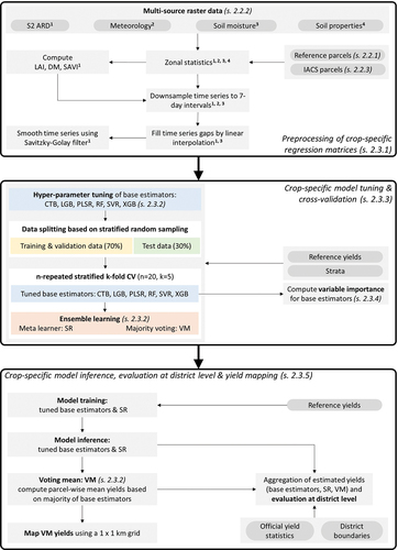
The flow chart shown in Figure 2 depicts the workflow followed in this study. The entire data preprocessing and modeling workflow has been fully implemented in Python (v3.9.16, VanRossum and Drake 2009) using the “Copernicus Data and Exploitation Platform – DE” (CODE-DE). CODE-DE is a bespoke EO cloud computing platform for German federal authorities and has comprehensive access to large repositories of satellite imagery, sizable computation resources, and integrated API functionalities for product dissemination. The platform is, thus, well suited for developing and providing scalable end-to-end EO applications.

Figure 2. Schematic shows adopted workflow of data preprocessing, modeling, and validation steps. Superscripts shown in upper box number multi-source raster data and link them to respective covariate preprocessing steps. DM: dry matter IACS: Integrated Administration and Control System, LAI: leaf area index, S2 ARD: Sentinel-2 analysis ready data, s.: section. CTB: CatBoost, LGB: LightGBM, PLSR: Partial Least Square, RF: Random Forest, SVR: Support Vector, XGB: XGBoost, SR: Stacking regressor, VM: Voting mean.

2.3.1. Data preprocessing

Geodata obtained from external data platforms were harmonized in terms of geographic projection (Figure 2). The extent of related raster data was constrained based on a vector shape of German national borders using the Python package “rasterio” (Gillies et al. 2013).

Parcel-wise processing included inward buffering of 10 m using the Python package “GeoPandas” (Jordahl et al. 2020), to exclude pixels with mixed reflectance signals present at parcel edges and typically caused by different land use or vegetation types. Zonal statistics was applied to extract mean values of included covariates for each parcel, using the Python package “rasterstats” (Perry 2023) (Figure 2). Multi-temporal EO satellite imagery generally provides irregular time series due to S2 revisiting time and observational gaps introduced by cloud masking. Hence, covariate time series based on S2 ARD imagery were temporally downsampled to regular time series by computing mean values over 7-day intervals with a total length of 22 7-day intervals, consistently covering a period, ranging from 1st of March to 31st of July for each included year. By focusing on this period, RS-based covariates capture vegetation signals of targeted winter crops during their transition from vegetative to reproductive and maturity phases of phenological development, where several factors, such as drought and heat stress, impact yield formation (Hlaváčová et al. 2018; Riedesel et al. 2023). Remaining gaps in covariate time series were imputed, applying a linear interpolation approach, using the Python package “pandas” (The pandas development team 2023). The Savitzky–Golay filter was applied to smooth $\mathit{LAI}$, $\mathit{DM}$, and $\mathit{SAVI}$ time series, mitigating the effect of signal contamination from cloud or cloud shadow remnants not removed by prior cloud masking using the “SciPy” package (Savitzky and Golay 1964; Virtanen et al. 2020). Filter parameters such as window length and polynomial smoothing order were set to 7 and 3, respectively. Meteorological data and $\mathit{SWI}$ were equally resampled, matching temporal resolution and length of time series derived from satellite imagery.

Regression matrices were generated for model training and inference, integrating preprocessed covariates for all parcels included (Figure 2). Regression matrices used for model training also included observed reference yields. While matrices generated for model training included all available yield references from 2018 to 2022, those matrices used for model inference to estimate crop yields for a large number of parcels across two federal states were created annually from 2019 to 2022. The year 2018 was excluded from inference due to the limited availability of reference data for this particular year ($N^{\mathrm{WW}}=64$, $N^{\mathrm{WB}}=3$, $N^{\mathrm{WR}}=47$).

2.3.2. ML-ensemble

Multiple supervised ML regression estimators suitable for data mining were chosen as base estimators for their ability to deal with high-dimensional covariate spaces and non-linear relations among variables. Base estimators, constituting the ML-ensemble (Figure 2), are Partial Least Square regressor (PLSR), Random Forest regressor (RF), and Support Vector regressor (SVR) included in the Python package “scikit-learn” (Pedregosa et al. 2011). In addition, Gradient Boosted Tree (GBT) regressors were used from the following Python packages “CatBoost” (CTB) (Dorogush, Ershov, and Gulin 2018), “LightGBM” (LGB) (Ke et al. 2017), and “XGBoost” (XGB) (Chen and Guestrin 2016). These estimators have previously been applied in a number of studies to model crop yields (Marshall et al. 2022; Shahhosseini et al. 2021; Srivastava et al. 2022; Uribeetxebarria, Castellón, and Aizpurua 2023).

In order to investigate techniques that are able to infer yields robustly at large spatial scales, over multiple years, and across different crop types, two ensemble learning techniques were assessed, each leveraging the full breadth of the ML-ensemble (Figure 2). First, model stacking was employed by utilizing a stacking regressor (SR), coalescing the entire ensemble of yield estimations generated by base estimators. The regularized linear regression approach Elastic Net regression (“scikit-learn”) was chosen as meta learner, seeking out the optimal bias-variance trade-off. Meta-learning capitalizes on the strengths of individual base estimators by learning from their outputs, providing a solution that may approach closely or even outperform estimates of those base estimators in the ML-ensemble showing the highest accuracies (Zhang, Liu, and Shen 2022). SR was trained using yield estimates predicted by base estimators, representing the meta-learner’s covariates. Second, mean yield estimates were computed for each parcel following the principle of majority voting (Zhang, Liu, and Shen 2022). The majority of estimated yields was determined by computing parcel-wise two-binned histograms based on the population of yields inferred by the base estimator ensemble (Figure 2). The histogram bin containing most of the yield estimates was chosen (voted for) and the mean of all yield estimates falling into that bin was calculated (voting mean = VM).

2.3.3. Model tuning and evaluation

This study followed established data splitting and cross-validation procedures to evaluate model ensembles (Piikki et al. 2021). Yield estimation models were tuned, trained, and validated crop specifically (Figure 2).

A Bayesian optimization approach was chosen for tuning hyper-parameters of base estimators following a sequential search ($\mathit{iterations}=200$) for optimal hyper-parameter combinations using the Python package “hyperopt” (Bergstra et al. 2015). In each iteration, mean values of root mean square errors ($\mathit{RMSE}$, eq. 1, Appendix B) were computed based on a repeated k-fold cross-validation procedure. $\mathit{RMSE}$ values served as input to the objective function updating the prior.

To evaluate tuned models, a stratified random sampling strategy was chosen for data splitting and cross-validation (Figure 2). Chosen strata represent major terrestrial and biophysically distinct regions across Germany differing in their geomorphological, climatic, and soil characteristics (Symank 1994). This dataset was chosen to ensure that reference data split into training, validation, and test chunks each proportionally consist of samples that represent these differences affecting crop management and productivity. Reference samples were distributed across strata 1 to 6 (Figure A1). The underlying vector dataset was accessed through the German Federal Agency for Nature Conservation (BfN 2023). Crop-specific regression matrices, including yield references and model covariates, were each split into two datasets based on a 70:30 ratio (Figure 2). This ratio was chosen to maintain reference samples across the strata and folds during the cross-validation procedure for all three crops. 70% of the data were used to evaluate the ensemble of base estimators by deploying an n-repeated stratified k-fold cross-validation scheme ($\mathit{n}=20$, $\mathit{k}=5$) based on training and validation folds. Hold-out sets (test) covering 30% of the data were set aside to evaluate yield estimates of the ensemble, including SR and VM, based on reference data that none of the estimators has been trained on during cross-validation. Descriptive statistics on reference data split into cross-validation and hold-out test sets are shown in Table 3.

Table 3. Descriptive statistics of yield reference data (t ha⁻¹) split into subsets used for cross-validation and hold-out (test) sets. WW: winter wheat; WB: winter barley; WR: winter rapeseed.

	WW		WB		WR
	cross val.	test	cross val.	test	cross val.	test
n	441	189	310	133	390	166
mean	7.62	7.86	7.25	7.30	3.68	3.71
std	1.93	2.07	2.16	2.18	0.88	0.90
min	1.96	3.00	1.20	1.88	0.84	1.52
25%	6.40	6.49	5.70	5.80	3.14	3.09
50%	7.83	7.98	7.58	7.18	3.76	3.77
75%	8.99	9.32	8.67	8.55	4.30	4.36
max	12.00	13.00	12.10	12.20	6.29	6.32

This cross-validation scheme has also been used to elicit model evaluation metrics for tuned base estimators and SR based on out-of-fold predictions (validation sets) and hold-out test sets (including VM) averaged over cross-validation runs (Figure 2). Out-of-fold yield estimates predicted by base estimators were used to train the meta-learner mitigating the risk of overfitting. In addition to $\mathit{RMSE}$, the set of evaluation metrics includes normalized root mean square error ($\mathit{nRMSE}$, eq. 2) and coefficient of determination ($\mathit{RSQ}$, eq. 3).

2.3.4. Assessment of variable importance

In order to interpret the importance of certain covariates on the inference skills of crop-specific model ensembles, variable importance (VIP, Figure 2) was assessed, following a two-step procedure. Prior to conducting the VIP, minimal sets of most relevant covariates were selected crop-specifically through decorrelation and recursive feature elimination (RFE) by applying XGB, included in the Python package “featurewiz” (Seshadri 2023). In featurewiz, the degree of correlation among covariates (multicollinearity) is determined by the Pearson’s correlation coefficient ($\mathit{r}$). The pre-set default threshold for high collinearity of $\mathit{r}=0.7$ was kept. In addition, mutual information scores (MIS) between covariates and reference yields were computed. Covariates exceeding the threshold for high collinearity and showing comparatively lower MIS were removed. Subsequently, permutation importance was used as VIP measure to determine the importance of each remaining covariate, using the model agnostic Python package “ELI5” (Korobov and Lopuhin 2021). Permutation importance measures the drop in $\mathit{RSQ}$ values after sequentially removing individual covariates from a model tasked with inference by replacing respective covariate values with random noise (Breiman 2001). Hence, permutation importance provides insights into how sensitive model inference skills are in regard to certain covariates. In this study, importance values were ascertained by deploying the full ensemble of base estimators imposing an n-repeated k-fold cross-validation scheme ($\mathit{n}=20$, $\mathit{k}=5$).

2.3.5. Large-scale yield estimation, evaluation at district level, and examples of high-resolution yield maps

Multi-year crop yields (2019–2022) were inferred for a large number of parcels (Table 1), deploying the tuned and trained ML-ensembles. Yield estimates derived from each base estimator, SR, and VM were individually aggregated at the district level by computing the mean crop-specific yield per district based on those parcels falling into a given district (Figure 2). Open vector data on administrative boundaries of districts located in Brandenburg and Lower Saxony were obtained from the German Federal Agency for Cartography and Geodesy (Federal Agency for Cartography and Geodesy 2022). Reported yields at the district level were linked to district features enabling the comparison of estimated mean yields and reported yields. Relative model biases ($\mathit{rBIAS}$, eq. 4) were computed to assess the degree of systematic deviation between estimated yields at district level and officially reported yields.

A systematic vector grid covering the study area was created at a spatial resolution of $1\times 1\mathrm{km}$, using QGIS. Parcel level yield estimates inferred by VM for 2021 were aggregated by computing means for each grid cell to provide examples of high-resolution yield maps (Figure 2) for targeted crops, using the Python package “GeoPandas” (Jordahl et al. 2020).

3. Results

3.1. Model cross-validation

Table 4 provides an overview of evaluation results for individual base estimators and ensemble learning techniques in regard to mean $\mathit{RSQ}$, $\mathit{nRMSE}$, and $\mathit{RMSE}$ metrics based on a repeated stratified cross-validation scheme and hold-out test data. The base estimator showing highest $\mathit{RSQ}$ and lowest $\mathit{nRMSE}$ values validated based on hold-out (test) sets is SVR for WW ($\mathit{RSQ}=0.76$, $\mathit{nRMSE}=12.8$%), WB ($\mathit{RSQ}=0.70$, $\mathit{nRMSE}=16.2$%), and WR ($\mathit{RSQ}=0.68$, $\mathit{nRMSE}=13.7$%). In contrast, lowest $\mathit{RSQ}$ and highest $\mathit{nRMSE}$ values based on test sets are indicated by RF for WW ($\mathit{RSQ}=0.69$, $\mathit{nRMSE}=14.7$%), PLSR for WB ($\mathit{RSQ}=0.65$, $\mathit{nRMSE}=17.6$%), and again RF for WR ($\mathit{RSQ}=0.59$, $\mathit{nRMSE}=15.3$%). Comparing the two ensemble learning techniques SR and VM against hold-out test data reveals only minor differences in accuracy metrics for all three crops. Both techniques show marginally inferior performances compared to the best-performing base estimator (Table 4).

Table 4. Overview of evaluation results for individual base estimators and ensemble learning techniques based on a repeated stratified cross-validation scheme. Underlying reference data were split into training (train) and validation (val) folds, and hold-out (test) sets. Bold values: best performing estimator per crop, italic values: least performing estimator per crop.

	RSQ			nRMSE (%)			RMSE (t ha^−1)
	WW	WB	WR	WW	WB	WR	WW	WB	WR
PLSR
train	0.81	0.84	0.77	10.91	11.91	11.39	0.83	0.86	0.42
val	0.73	0.68	0.69	13.11	16.51	13.13	1.00	1.19	0.48
test	0.75	0.65	0.67	13.05	17.64	13.86	1.03	1.29	0.51
SVR
train	0.89	0.85	0.80	8.49	11.57	10.79	0.65	0.84	0.40
val	0.75	0.70	0.68	12.64	15.92	13.27	0.96	1.15	0.49
test	0.76	0.70	0.68	12.76	16.18	13.71	1.00	1.18	0.51
RF
train	0.80	0.92	0.82	11.26	8.37	10.06	0.86	0.61	0.37
val	0.80	0.67	0.61	11.24	16.68	14.72	0.86	1.21	0.54
test	0.69	0.65	0.59	14.66	17.60	15.32	1.15	1.28	0.57
CTB
train	0.85	0.86	0.79	9.62	11.15	10.90	0.73	0.81	0.40
val	0.74	0.69	0.64	12.85	16.19	14.26	0.98	1.17	0.52
test	0.73	0.66	0.64	13.67	17.31	14.45	1.07	1.26	0.54
LGB
train	0.92	0.91	0.73	7.13	8.93	12.41	0.54	0.65	0.46
val	0.75	0.69	0.61	12.65	16.14	14.75	0.96	1.17	0.54
test	0.72	0.67	0.63	13.83	17.13	14.68	1.09	1.25	0.55
XGB
train	0.90	0.89	0.89	7.86	9.69	7.88	0.60	0.70	0.29
val	0.74	0.70	0.66	12.76	16.02	13.79	0.97	1.16	0.51
test	0.72	0.67	0.65	13.93	17.24	14.31	1.10	1.26	0.53
SR
train	0.84	0.75	0.72	9.92	14.57	12.57	0.76	1.05	0.46
test	0.73	0.69	0.67	13.78	16.58	13.84	1.08	1.21	0.51
VM
test	0.74	0.68	0.66	13.42	16.85	14.09	1.06	1.23	0.52

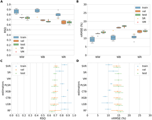
Evaluation results of the model ensemble are illustrated in terms of $\mathit{RSQ}$ and $\mathit{nRMSE}$ metrics by crop and estimator in Figure 3. Base estimator ensemble medians of validation metrics computed based on hold-out (test) sets are: $\mathit{RSQ}=0.73$, $\mathit{nRMSE}=13.7$%, for WW, $\mathit{RSQ}=0.66$, $\mathit{nRMSE}=17.3$% for WB, and $\mathit{RSQ}=0.64$, $\mathit{nRMSE}=14.4$% for WR (Figure 3a,b). Comparing these ensemble medians against the metrics obtained from two ensemble learning techniques reveals that particularly VM did slightly outperform the base estimator ensemble across crops. Estimators yielding the highest and lowest mean $\mathit{RSQ}$ and $\mathit{nRMSE}$ across all three crops are SVR ($\mathit{RSQ}=0.72$, $\mathit{nRMSE}=14.2$%) and RF ($\mathit{RSQ}=0.65$, $\mathit{nRMSE}=15.9$%), respectively, evaluated based on test sets (Figure 3c,d). Ensemble medians of $\mathit{RSQ}$ and $\mathit{nRMSE}$ obtained from hold-out test sets compared to validation folds are slightly inferior for WW and WB and similar for WR (Figure 3a,b). Marginally lower and similar model performances on hold-out test sets do suggest that generalization skills of the ensemble do not depress notably when confronted with unseen data.

Figure 3. ML-ensemble evaluation results based on a repeated stratified cross-validation scheme. Underlying yield reference data were split into training (train) and validation (val) folds and hold-out (test) sets. $\mathit{RSQ}$ and $\mathit{nRMSE}$ plots are shown by crop type (A and B) and by estimator (C and D), where bars around means represent standard deviations. WW: winter wheat, WB: winter barley, WR: winter rapeseed. Evaluated ML-ensembles consist of six base estimators (CTB, LGB, PLSR, RF, SVR, and XGB) and two ensemble learning techniques, represented by meta learner (SR) and voting mean based on majority voting (VM).

3.2. Variable importance analysis

Permutation importance boxplots of the five most important covariates (TOP 5) based on the whole ensemble of base estimators depict predominantly EO-based covariates for all three crop (Figure 4). Median $\mathit{RSQ}$ values react most sensitive to the removal of spectral covariates related to included $\mathit{SAVI}$ and biophysical crop traits $\mathit{LAI}$ and $\mathit{DM}$ by dropping up to 0.22 for WW, 0.12 for WB, and 0.13 for WR, respectively. $\mathit{SAVI}$ and $\mathit{LAI}$ covariates show the highest importance in late May and late June for WW (Figure 4a). $\mathit{LAI}$ and $\mathit{DM}$ covariates are most important in late April, late May, and mid-June for WB (Figure 4b). $\mathit{LAI}$ and $\mathit{DM}$ covariates indicate highest importance in early May and early to mid-June for WR (Figure 4c). In addition, yield estimates of WW are shown to be influenced by longitude ($\mathit{X}$), indicating a West to East gradient of decreasing yield levels (see Figure A3). The high importance of VI and biophysical crop traits between the end of April and the end of June fall into the main crop development phase of crop reproduction and yield formation represented by principal growth stages (BBCH-scale) of heading and fruit development for WW, flowering and fruit development for WB, and flowering as well as pod and seed development for WR.

Figure 4. Overview of five most important covariates computed by running permutation importance analyses based on all six base estimators, forming the ML-ensembles shown for A) winter wheat (WW), B) winter barley (WB), and C) winter rapeseed (WR). DM: dry matter, LAI: leaf area index, pH: soil pH, SAVI: soil adjusted vegetation index, X: longitude. Covariate labels include date information [mm-dd], indicating month and trailing day of respective 7-day period.

3.3. Comparing estimated yields at district level against officially reported yields

Figure 5 shows $\mathit{RSQ}$ and $\mathit{nRMSE}$ metrics, illustrating a multi-year model evaluation from 2019 to 2022 for base estimators at the district level. In addition, $\mathit{RSQ}$ and $\mathit{nRMSE}$ values are plotted on top of each box for ensemble learning techniques SR and VM (Figure 5a,b). Median $\mathit{RSQ}$ and $\mathit{nRMSE}$ values derived from the ensemble of base estimators range between 0.78–0.89 and 7.3–8.6% for WW, 0.79–0.82 and 6.4–10.0% for WB, and 0.58–0.77 and 6.3–10.6% for WR, respectively, across years (Figure 5a,b). It is noticeable that $\mathit{RSQ}$ medians range firmly between 0.70 and 0.90 across crops and years, except for WR in 2020, where a clear drop is visible. The respective $\mathit{nRMSE}$ median is not elevated, though.

Figure 5. Evaluation of ensemble yield estimations aggregated at district level and compared against official yield reports. $\mathit{RSQ}$ and $\mathit{nRMSE}$ plots are shown by crop type (A and B) and by estimator (C and D), where bars around means represent standard deviations. WW: winter wheat, WB: winter barley, WR: winter rapeseed. Evaluated ML-ensembles consist of six base estimators (CTB, LGB, PLSR, RF, SVR, and XGB) and two ensemble learning techniques, represented by meta learner (SR) and voting mean based on majority voting (VM).

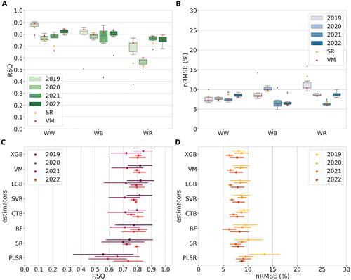
$\mathit{RSQ}$ and $\mathit{nRMSE}$ values obtained from evaluating aggregated yields estimated through meta-learning (SR) are 0.70–0.85 and 7.9–9.0% for WW, 0.75–0.82 and 6.6–9.6% for WB, and 0.53–0.78 and 6.8–13.3% for WR, respectively. Evaluating aggregated yields elicited by computing VM based on majority voting led to $\mathit{RSQ}$ and $\mathit{nRMSE}$ values of 0.79–0.89 and 7.2–8.1% for WW ($\mathit{RMSE}=0.50-0.61$ t ha⁻¹), 0.80–0.84 and 6.0–9.9% for WB ($\mathit{RMSE}=0.40-0.66$ t ha⁻¹), and 0.60–0.78 and 6.1–10.4% for WR ($\mathit{RMSE}=0.20-0.34$ t ha⁻¹), respectively (Figure 5a,b). Comparing evaluation metrics obtained from ensemble medians and the two ensemble learning techniques SR and VM overall indicates a slightly superior performance of VM across crops. Highest mean $\mathit{RSQ}$ and lowest mean $\mathit{nRMSE}$ values across crops and years are shown for XGB and VM having equal values for $\mathit{RSQ}=0.79$ and $\mathit{nRMSE}=7.8$%. The estimator indicating lowest mean $\mathit{RSQ}$ and highest mean $\mathit{nRMSE}$ values across crops is PLSR with $\mathit{RSQ}=0.63$ and $\mathit{nRMSE}=10.2$% (Figure 5c,d).

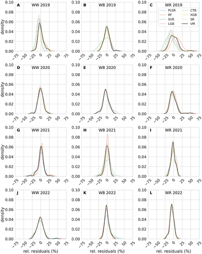
Density plots in Figure 6 provide an overview of relative model residuals, that is, the relative deviation between mean yield estimates at the district level and official yield reports at the district level per crop and year. Overall, the density distribution of relative residuals for base estimators, SR, and VM centers around 0. Median residuals for most of the base estimators, SR, and VM range below $\pm$10% as expected given $\mathit{nRMSE}$ values illustrated in Figure 5d. However, for WR in 2019 (Figure 6c), median residuals of −10% are exceeded by PLSR (−11.9%). In a few cases, such as for WW in 2022 and WR in 2019 and 2020, relative residuals derived from VM are as high as 50% or above for a very low number of districts, indicated by marginal density values at those residual levels (Figure 6c,f,j). Related scatter plots can be found in Appendix A (Figure A2). The lowest mean $\mathit{rBIAS}$ across crops and years is shown for RF (0.6%), followed by VM and XGB (−1.3%) In contrast, the highest mean $\mathit{rBIAS}$ is indicated for PLSR (−3.0%).

Figure 6. Distribution densities of relative model residuals (%) at district level (aggregated mean yield estimates – official yield reports) for the whole ensemble, shown by year (rows) and crop (columns). WW: winter wheat, WB: winter barley, WR: winter rapeseed.

3.4. Use of ensemble-based majority voting for high-resolution crop yield mapping

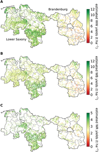
Mean crop yields estimated by utilizing ensemble learning-based VM are mapped per crop for 2021 based on a $1\times 1\mathrm{km}$ grid providing examples of high-resolution crop yield maps (Figure 7). These maps show pronounced spatial differences in yield levels for all three crops. Relatively high yielding regions are predominantly located in Southern Lower Saxony. In contrast, lower yielding areas are spread across Brandenburg. Spatial yield variability inside districts is depicted as well. For instance, the maps reveal that districts located in the Northern regions of Brandenburg and Lower Saxony harbor areas with notably varying yield levels.

Figure 7. Estimated mean crop yields for 2021 derived from majority voting (VM), mapped for A) WW (winter wheat), b) WB (winter barley), and C) WR (winter rapeseed) on a $1\times 1\mathrm{km}$ grid. Boundaries delineate districts (NUTS 3).

4. Discussion

4.1. Robustness of ensemble-based yield estimation at different spatial scales

In this study, ensembles of six base estimators and two ensemble learning techniques have been used to estimate yields at scale for three major crops in Germany. A repeated stratified cross-validation scheme revealed no discernible difference between ensemble learning techniques SR and VM, given similar evaluation metrics based on hold-out test data (Table 4). In contrast, when evaluating aggregated yield estimates derived from ensemble learning techniques against official yield statistics, the inference skills of VM outperformed SR (Figure 5). Evaluation metrics yielded for VM were also slightly superior compared to medians of base estimator ensembles obtained from cross-validations and district level comparisons across crops (Figures 3a,b, 5a,b). Hence, the superior inference skills of VM compared to SR (Figure 5) and above ensemble median performance suggest improved yield estimation robustness of this ensemble learning technique, providing justification to focus on VM henceforth.

A number of localized studies have been conducted recently to estimate yields of WW, WB, and WR at the parcel level and below across Europe, applying similar ML-based approaches, yet with varying model structures and covariates. An overview of evaluation metrics obtained from the related literature is provided in Table 5 to benchmark cross-validation results derived for VM.

Table 5. Overview of validation metrics reported in this study benchmarked against metrics obtained from recent literature, conducting comparable modeling exercises. Comparisons are grouped into spatial scales, ranging from local to administrative levels. Displayed metrics referring to this study are derived from cross-validation at parcel level against test sets and multi-annual district-level evaluation against official yield reports for ensemble learning-based majority voting (VM). ${ }^{\star }$Values represent mean absolute percentage errors and ${ }^{\star \star }$values reflect mean absolute errors due to absent reporting of $\mathit{nRMSE}$ and $\mathit{RMSE}$ values.

	RSQ			nRMSE (%)			RMSE (t ha^−1)
Spatial scale	WW	WB	WR	WW	WB	WR	WW	WB	WR
Parcel level and below
this study (VM)	0.74	0.68	0.66	13.4	16.9	14.1	1.06	1.23	0.52
Ghosh et al. (2022)	0.65	0.69	0.86	16.5	20.6	32.5	1.38	1.56	1.12
Perich et al. (2023)	0.65–0.86	–	–	10.5–17.8	–	–	0.66–1.12	–	–
Uribeetxebarria et al. 2023)	0.50–0.95	–	–	3.5–15.3	–	–	0.24–1.10	–	–
Administrative levels
this study (VM)	0.79–0.89	0.80–0.84	0.60–0.78	7.2–8.1	6.0–9.9	6.1–10.4	0.50–0.61	0.40–0.66	0.20–0.34
Dhillon et al. (2023)	0.91	–	0.84	7.3	–	8.8	0.50	–	0.21
Srivastava et al. 2022)	0.65–0.81	–	–	–	–	–	0.64–0.84	–	–
Bognár et al. (2022)	0.81	–	0.67	${ }^{\star }$7.6	–	${ }^{\star }$14.4	${ }^{\star \star }$0.32	–	${ }^{\star \star }$0.31
Mateo-Sanchis et al. (2021)	0.85	0.84	–	–	–	–	0.78	0.75	–

Based on data from 2017, Ghosh et al. (2022) estimated crop yields for WW, WB, and WR at parcel level ($N^{\mathrm{WW}}=149$, $N^{\mathrm{WB}}=144$, $N^{\mathrm{WR}}=66$) in Hesse, Germany. RF was used, fed with combined covariates derived from SAR (S1) and multi-spectral imagery (S2). Validation results shown in Table 5 suggest a similar modelling performance to the one reported in this study. However, mean yield estimation errors ($\mathit{nRMSE}$) obtained by Ghosh et al. (2022) were in general shown to be higher for all three crops, particularly for WR.

Perich et al. (2023) modeled WW yields multi-annually (2017–2021) at parcel level ($\mathit{n}=19$) in Switzerland. An artificial neural network was trained with covariates based on multi-spectral S2 time series data. Yielded validation results suggest a comparable modeling performance to the one derived in this study (Table 5).

Using data from 2021, Uribeetxebarria et al. (2023) estimated yields for WW at parcel level ($\mathit{n}=39$) in Spain based on various ML algorithms such as RF, SVR, and CTB. Covariates used, included a range of VIs based on multi-spectral S2 imagery and dual-pol SAR-normalized backscatter features (S1). Particularly, the CTB model showed a superior performance compared to the ensemble used in this study when jointly fed with S1- and S2-derived covariates (Table 5).

Aggregated VM yields were compared against official crop yield reports at the district level over two federal states and four consecutive years (2019–2022). A range of yield estimation studies have been conducted at various coarser administrative levels, reporting validation metrics shown in Table 5.

Dhillon et al. (2023) estimated WW and WR yields for 2019 at district level (NUTS 3), focusing on the federal state of Bavaria located in Southern Germany. A hybrid approach was applied, using a process-based light use efficiency approach coupled with RF. Covariates included above-ground biomass simulated based on synthesized MODIS and S2 imagery, and a number of meteorological variables. Accuracy metrics for best-performing models shown in Table 5 indicate a similar model performance compared to multi-year validation results based on VM presented in this study. The on-par performance corroborates the robustness of the ensemble learning-based approach followed in this study across years and crops.

Srivastava et al. (2022) estimated WW yields multi-annually (2017–2019) at district level (NUTS 3) in Germany, using various ML and deep learning models. These models were fed with meteorological-, soil-, and phenology-related covariates. A convolutional neural network (CNN) outperformed ML approaches yielding validation results shown in Table 5. Compared to the validation results obtained based on VM in this study, the results of Srivastava et al. (2022) are shown to be slightly inferior, suggesting that yield estimation at the parcel level may improve the validity of aggregated estimates at higher administrate levels such as districts.

Bognár et al. (2022) conducted a modeling study at county level (NUTS 3) in Hungary estimating crop yields for WW and WR in 2020. Various VIs derived from MODIS imagery were tested by comparing the integral of VI time series against reported yields at district level. The best performing VI integral yielded validation results depicted in Table 5. Given that mean absolute percentage errors and mean absolute errors reported by Bognár et al. (2022) are generally lower than corresponding $\mathit{nRMSE}$ and $\mathit{RMSE}$ values (not reported), ensemble-based validation results reported in this study are of similar or even superior goodness.

Mateo-Sanchis et al. (2021) did a European-wide yield estimation exercise at administrative level (NUTS 2) for WW and WB. A variety of covariates was integrated into a Gaussian Process regression model, including a VI, $\mathit{LAI}$, $\mathit{SSM}$, and gridded meteorological variables to estimate crop yields from 2015 to 2017. Multi-annual ranges of obtained validation metrics are provided in Table 5. Although $\mathit{RSQ}$ values reported by Mateo-Sanchis et al. (2021) are comparable to the ones shown in this study, modeling errors ($\mathit{RMSE}$) for WW and WB are continuously higher, suggesting lower uncertainty of bottom-up scaled yield estimation as proposed in this study. Bottom-up yield estimation approaches based on crop growth modeling have been demonstrated to be more robust compared to frameworks that rely on large-scale yet spatially less granular datasets (Rattalino et al. 2021; van Bussel Lenny et al. 2015).

Crop yields estimated by using ensemble learning-based majority voting deviated between 13–17% and 6–10% from reference yields and official yield reports at the district level, respectively (Table 5). Such accuracy levels can be deemed sufficient to reliably infer statistics on crop productivity given the variability of reported yields present at administrative levels. Multi-annual ranges (2019–2022) of standard deviations ($\mathit{std}$) on reported yields at district level for the study region are $\mathit{std}=16-22$% for WW, $\mathit{std}=15-22$% for WB, and $\mathit{std}=13-20$% for WR. However, caution should be taken when inferring statistics based on modeled yield estimates from those regions where reference data used for model training are lacking. Example maps in Figure 7 reveal details on spatial yield variability at even higher granularity ($1\times 1\mathrm{km}$ resolution). Visually, depicted patterns show high agreement with the spatial variability of cropland yield potential in Germany based on the Muencheberg Soil Quality Rating (Federal Institute for Geosciences and Natural Resources 2014). In light of the presented results, ensemble learning-based majority voting may represent a suitable strategy to estimate crop yields robustly across spatial scales ranging from individual parcels to administrative units covering larger regions.

4.2. Model interpretability

Most important covariates across crops link to the VI and biophysical crop traits retrieved from multi-spectral vegetation signals during the reproductive phase of crops’ phenological developments, as revealed from conducting a VIP. $\mathit{SAVI}$ time series applied in this study are shown to have a high influence on yield estimation during reproductive crop growth phases of fruit and pod development confirming similar findings reported previously (Croci et al. 2023; Nagy et al. 2021).

In this study, regression coefficients derived from statistical modeling by using a hyper-spectral crop library enabled the space-borne retrieval of $\mathit{LAI}$ and $\mathit{DM}$. Marshall et al. (2022) reported superior performance of ML models estimating WW yields at farm scale when feeding covariates based on multi- and hyper-spectral satellite imagery at the reproductive phase in contrast to vegetative and maturity phases of phenological development. Paudel et al. (2023) showed the highest importance of $\mathit{LAI}$ and crop biomass covariates elicited from crop growth modeling and fed into deep learning models forecasting water-limited WW yields at national scale for the reproductive phase, in particular during flowering and yield formation.

These findings underline the role of VIs and biophysical crop traits, serving as spectral yield indicators during crops’ reproductive development phases (cf. Johnson 2016). During this period, plant canopies reach peak productivity and chlorophyll absorption levels are highest. Reproductive organs are being developed, inducing translocation of assimilate from plant to grain and pod development before photosynthetic activities slow down while transitioning toward crop maturity (Marshall et al. 2022).

Moreover, longitude ($\mathit{X}$) entails information on yield estimates for WW reflecting decreasing yields following a general gradient from West to East. Such gradient is prevalent in the underlying in-situ reference dataset (see Figure A3) and represents a surrogate for changing soil-climatic conditions, determining crop growth potentials along the West to East axis (cf. DLO 2011).

Included meteorological and soil data do not rank among the most important covariates (TOP 5) except for $\mathit{pH}$ (WR). Reasons for the lower importance of these covariates for yield estimations may relate to coarser spatial resolutions of underlying datasets compared to S2 imagery, hence, bearing lower spatial variability at the parcel level. Moreover, gridded meteorological and soil data are generated through spatial modeling of weather station and soil profile data (cf. Poggio et al. 2021), thus, introducing uncertainties around resulting estimates.

4.3. The added value of a scalable yield estimation approach

The ensemble learning-based approach presented in this study may improve the production of agricultural crop yield statistics. Underlying EO satellite imagery, gridded meteorological, and soil data ensure timeliness and completeness of such approaches due to near real-time data availability and comprehensive data coverage of cultivation areas. Detailed yield maps covering the entire country could inform decision-making processes at a spatial resolution unprecedented so far. The finest granularity of officially reported crop yield data is NUTS 3 level corresponding to districts in Germany (Destatis and state offices for statistics 2023). By using the approach proposed and tested in this study operationally, crop yields could be made available using a systematic $1\times 1\mathrm{km}$ grid (see Figure 7). Using map services such as Destatis’ regional statistics atlas (Destatis 2023c) and interface standards such as Web Map Service (WMS) and WCS, parcel-level crop yield estimates could lay the foundation for providing dynamic data products based on spatial and temporal aggregation functionalities (cf. Wagemann et al. 2018).

Such data products would be tailored to meet the needs of stakeholders that seek to inform their decision-making processes at various scales, for instance, benefiting spatially explicit crop failure compensation or regional yield monitoring (cf. Meitner et al. 2023; Paudel et al. 2022). In addition, a scalable yield estimation approach potentially provides added value for comprehensive analyses at a large spatial scale, yet high spatial resolution on the nexus of food production systems, biodiversity, and climate change, informing sustainable land use governance (cf. Chaudhary, Pfister, and Hellweg 2016; Prestele and Verburg 2020).

Furthermore, implementing the approach operationally may lower monetary costs accrued from regular field and survey campaigns conducted annually by mandated authorities to elicit yield reports at administrative levels. This could be achieved by informing the sampling design in such a way that yield reference data are collected annually with reduced sampling density or related campaigns are conducted at a lower frequency, for instance in two- or three-year intervals.

4.4. Present caveats

Geolocalized yield reference data at parcel level distributed over larger geographical regions such as federal states or an entire country are generally scarce and sensitive in nature. A comparatively sizable reference dataset, covering several years and regions, could be utilized for this study due to collaborations with statistical state offices and farmers. However, this dataset possesses a rather small sample size given the scaling purpose of this study and is, moreover, temporally and spatially unbalanced.

Therefore, more comprehensive, multi-temporal reference data for model training derived from stratified random sampling, taking into account agro-climatic and soil variability across Germany, could further improve generalizability and, hence, increase the robustness of ensemble inferences at scale. A soil-climatic zoning characterizing production areas for major crops cultivated in Germany has been introduced and could inform such a stratified sampling design (Graf et al. 2009).

Voluntary reporting networks, commonly drawn upon by statistical state offices, are increasingly difficult to maintain with sufficient geographic coverage and density. Citizen science approaches leveraging sensor-based yield approximations commonly found on board of modern harvesters may help enrich the yield reference database (cf. Deines et al. 2021). Particularly, the younger generation of farmers, often showing fast uptake of novel technology, could be attracted to participate in voluntary reporting networks, supporting agricultural statistics by contributing sensor-based yields mapped locally while harvesting. High-quality yield maps obtained through crowdsourcing require technological standards (eg. sensor platforms and APIs) and expertise to apply underlying technologies in a targeted fashion, though (Senaratne et al. 2017).

4.5. Outlook on potential improvements

Multi-temporal imagery from passive, optical satellite sensors such as S2 is prone to decreased observational densities due to cloud cover. Using harmonized multi-sensor imagery obtained from Landsat 8, 9, and S2 would provide additional satellite observations and, thus, may alleviate the impact of cloud cover on time series density to a certain extent. To do so, time series based on harmonized Landsat and S2 imagery, derived from the “Framework for Operational Radiometric Correction for Environmental Monitoring” (FORCE), could be incorporated (Frantz 2019). In addition, the integration of S1 SAR backscatter data should be pursued, since SAR signals penetrate cloud layers. SAR backscatter time series may, therefore, compensate for the loss of information caused by cloud cover when integrated into ML models, compared to models, that are fed with time series of crop biophysical traits and VIs derived from optical sensors alone (Hosseini et al. 2019; Uribeetxebarria, Castellón, and Aizpurua 2023).

Various climatic conditions across larger regions and climatic variability over time impact crops’ phenological cycles, leading to different planting and harvest dates (Bojanowski et al. 2022; Kerner et al. 2022; Möller, Boutarfa, and Strassemeyer 2020). As a result, temporal offsets may occur in multi-annual regression matrices fed into models for training and inference, potentially affecting yield estimation models’ ability to generalize patterns. Hence, normalizing time series phenologically by aligning their start and endpoints to parcel level key events such as crop emergence and harvest rather than using absolute calendar dates could reduce these offsets. This would also enable deriving phenological metrics by linking accumulated thermal time and vegetation signals from satellite observations (Skakun et al. 2019). An automated detection of such key events requires available geodata on phenological development phases. Spatially explicit time series datasets based on interpolated observations of phenological events are available for Germany. These datasets have been used to characterize phenological windows (Möller, Boutarfa, and Strassemeyer 2020), to calculate phenological and phase-specific weather indices (Möller et al. 2019), and to disentangle extreme weather effects on crop yields (Bucheli, Dalhaus, and Finger 2022; Riedesel et al. 2023, 2024).

However, due to their interpolated nature and relatively coarse spatial resolution, these datasets do not capture parcel-specific phase onsets, hence, introducing uncertainties at the parcel level. The development of EO-based approaches to generate phenological data products at high spatial resolution, using S1 and S2, has been gaining momentum lately (Gao and Zhang 2021; Misra, Cawkwell, and Wingler 2020; Veloso et al. 2017). Once available at scale, such products could play a crucial role in improving the scalable crop yield estimation approach at the parcel level.

The inclusion of additional winter and summer crops into the yield estimation approach is a logical step going forward. JKI’s hyper-spectral crop library “MISPEL” harbors crop-specific data for a number of additional candidate crops suitable for $\mathit{LAI}$ and $\mathit{DM}$ retrieval from multi-temporal satellite imagery as well as additional crop traits potentially relevant for crop yield estimation such as crop height and fresh above-ground biomass (Borrmann, Brandt, and Gerighausen 2023). Expanding the approach by covering a broader range of crops is required to support agricultural statistics more comprehensively.

Deep learning approaches such as CNNs and long short-term memory recurrent neural networks (LSTM-RNN) become tangible for high-resolution crop yield estimation at scale once a larger set of geolocated yield reference data is available. When used for crop yield estimation, CNNs and LSTM-RNNs have been shown to possess the capability of outperforming other ML algorithms (Khaki, Wang, and Archontoulis 2020; Shook et al. 2021; Srivastava et al. 2022).

A similar approach to the one presented in this study could be utilized for in-season crop yield forecasting at high spatial resolution by employing ML-ensembles trained crop specifically. Agricultural productivity assessments based on in-season crop yield forecasting are in high demand (cf. Bojanowski et al. 2022; Paudel, de Wit, et al. 2023). Such assessments could feed into agricultural statistics providing early harvest outlooks and risk measures to inform forward-looking food security assessments as well as crop insurance and compensation schemes (He et al. 2019; Ozaki et al. 2008). However, a longer period of yield reference data than the one available for this study is required to sufficiently incorporate inter-annual, particularly meteorological, variability (Conradt 2022).

5. Conclusions

This study proposes a novel ML-ensemble learning-based approach for scalable crop yield estimation based on a large number of parcels, validated for three major winter crops across two German federal states. The multi-year estimation of crop yields has been shown to generate robust results based on majority voting, suggesting operational utility for supporting agricultural statistics.

In addition, crop traits such as multi-temporal estimates on $\mathit{LAI}$ and $\mathit{DM}$ derived from EO imagery have been shown to represent cornerstones for the yield estimation approach presented, generally contributing most of the information to model outcomes. This clearly demonstrates the potential of space-borne vegetation monitoring for estimating crop yields at high spatial resolution and at a large spatial scale.

Further research should focus on integrating additional EO sensors such as Landsat 8, 9, and S1 to densify existing covariate time series for $\mathit{LAI}$ and $\mathit{DM}$ and to complement SAR backscatter time series. The use of additional sensors would also enable an accurate detection of phenological key events, allowing for a parcel-specific phenological normalization of covariate time series.

Implementing a scalable yield estimation approach into crop yield reporting frameworks of public authorities mandated to provide agricultural statistics would increase the spatial resolution of annually reported yield data, eventually covering the entire cropland available. Presented examples of high-resolution yield maps based on a $1\times 1\mathrm{km}$ grid may precurse unprecedented data products on crop productivity as part of official agricultural statistics. Delivered through appropriate map services, these data products could improve decision-making support for a range of stakeholders across different spatial scales, ranging from parcel to higher administrative levels.

Author contributions

Patric Brandt: Data curation, methodology, formal analysis, visualization, writing – original draft, and writing – review & editing. Florian Beyer: Data curation, methodology, and writing – review & editing. Peter Borrmann: Data curation, methodology, and writing – review & editing. Markus Möller: conceptualization and writing – review & editing. Heike Gerighausen: Supervision, conceptualization, writing – review & editing, project administration, and funding acquisition.

Acknowledgments

We like to thank the German Federal Statistical Office (Destatis) for funding the SatAgrarStat PLUS project. We are sincerely thankful for yield reference data provided by six German state offices for statistics (Bavaria, Brandenburg, Hesse, Lower Saxony, North Rhine-Westphalia, and Schleswig-Holstein) and numerous voluntary farmers, participating in the SatAgrarStat and MoNi (grant number 2820ABS001) projects. We also thank the German Meteorological Service (DWD) for making daily meteorological data available. Lastly, we thank the operators of CODE-DE for providing a tailored EO cloud computing platform for public organizations.

Supplementary Material

Supplemental data for this article can be accessed online at https://doi.org/10.1080/15481603.2024.2367808

Disclosure statement

No potential conflict of interest was reported by the author(s).

Data availability statement

Due to the sensitive nature and related data privacy regulations regarding yield reference data used in this study, involved farmers and statistical offices were assured that their data would remain confidential and not be shared. Data on estimated crop yields at the grid or district level will be made available upon request.

Additional information

Funding

This work was funded by the German Federal Statistical Office (Destatis).

Appendix A.

Supplementary tables & figures

Figure A1. Biophysical distinct regions in Germany used to stratify crop-specific reference data.

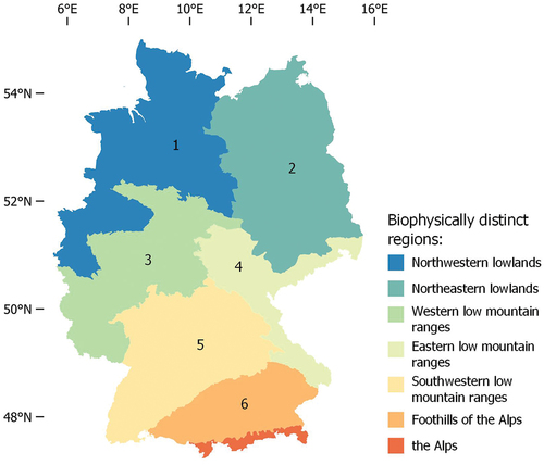
Figure A2. Scatter plots depict official yield statistics mapped against estimated yields aggregated at district level derived from majority voting (VM), shown by year (rows) and crop (columns). WW: winter wheat, WB: winter barley, WR: winter rapeseed. Dashed diagonals represent identity lines.

Figure A3. Relationship between longitude and reference crop yields for WW (A). Bavaria (BV), Brandenburg (BB), Hesse (HE), Lower Saxony (LS), North Rhine-Westphalia (NRW), and Schleswig-Holstein (SH).

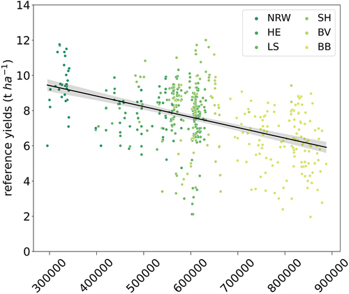
Table A1. Origin of reference data used for model training shown by year. Abbreviations of federal states: Bavaria (BV), Brandenburg (BB), Hesse (HE), Lower Saxony (LS), North Rhine-Westphalia (NRW), and Schleswig-Holstein (SH).

Crop		Years
	Federal state	2018	2019	2020	2021	2022
WW	BB	–	–	63	69	43
	BV	13	12	9	13	10
	HE	16	15	15	13	14
	LS	21	36	30	55	28
	NRW	1	1	13	23	14
	SH	13	10	17	25	38
WB	BB	–	–	48	57	37
	BV	–	2	4	7	5
	HE	–	–	14	12	12
	LS	3	9	47	48	48
	NRW	–	–	10	12	9
	SH	–	1	11	21	26
WR	BB	–	–	52	62	47
	BV	11	9	10	7	7
	HE	12	9	11	5	5
	LS	15	11	28	41	45
	NRW	–	–	3	2	6
	SH	9	9	49	39	52

Appendix B.

Model evaluation metrics

(B1) $\mathit{RMSE}=\sqrt{\frac{{\sum }_{i=1}^n{(y_i-x_i)}^2}{\mathit{n}}},$(B1)

(B2) $\mathit{nRMSE}=\frac{\mathit{RMSE}}{\bar{x}}\times 100,$(B2)

(B3) $\mathit{RSQ}=1-\frac{{\sum }_{i=1}^n{(x_i-y_i)}^2}{{\sum }_{i=1}^n{(x_i-\bar{x})}^2},$(B3)

(B4) $\mathit{rBIAS}=\frac{{\sum }_{i=1}^n\frac{(y_i-x_i)}{\bar{x}}\times 100}{\mathit{n}}$(B4)

where $x_i$ corresponds to observed crop yield obtained from reference data or official crop yield reports; $\bar{x}$ symbolizes mean observed crop yields; $y_i$ indicates model estimated crop yield; and $\mathit{n}$ represents the number of observations.

References

- Arnold, J., P. Brandt, and H. Gerighausen. 2021. “Testing of Satellite-Based Yield Estimation for Agricultural Statistics - the SatAgrarstat Project.” WISTA 6:1–29. Accessed June 12, 2023. https://www.destatis.de/DE/Methoden/WISTA-Wirtschaft-und-Statistik/2021/06/erprobung-satellitengestuetzte-ertragsschaetzung-062021.pdf?__blob=publicationFile.
- Bauer-Marschallinger, B., and S. Massart. 2023. Copernicus Global Land Operations “Vegetation and Energy, CGLOPS-1”. Quality Assessment Report. Update 2022. Soil Water Index Collection 1km. Version 1.0. Technical Report I1.00. TU Wien. https://land.copernicus.eu/global/sites/cgls.vito.be/files/products/CGLOPS1_QAR2022_SWI1km_V1_I1.00.pdf.
- Bauer-Marschallinger, B., C. Paulik, S. Hochstöger, T. Mistelbauer, S. Modanesi, L. Ciabatta, C. Massari, L. Brocca, and W. Wagner. 2018. “Soil Moisture from Fusion of Scatterometer and SAR: Closing the Scale Gap with Temporal Filtering.” Remote Sensing 10 (7): 1030. Accessed December 7, 2022. https://doi.org/10.3390/rs10071030.
- Baumann, P. 2021. “A General Conceptual Framework for Multi-Dimensional Spatio-Temporal Data Sets.” Environmental Modelling & Software 143:105096. Accessed October 19, 2023. https://doi.org/10.1016/j.envsoft.2021.105096.
- Bergstra, J., B. Komer, C. Eliasmith, D. Yamins, and D. D. Cox. 2015. “Hyperopt: A Python Library for Model Selection and Hyperparameter Optimization.” Computational Science & Discovery 8 (1): 014008. Accessed November 22, 2022. https://iopscience.iop.org/article/10.1088/1749-4699/8/1/014008/meta.
- Beyer, F., P. Brandt, M. Schmidt, U. Stahl, B. Golla, H. Gerighausen, and M. Möller. 2023. “A Paradigm Shift Towards Decentralized Cloud-Integrated Spatial Data Infrastructures: Lessons Learned and Solutions Provided for Public Authorities.” Accessed October 19, 2023. https://eartharxiv.org/repository/view/5494/.
- BfN. 2023. “Maps and Data.” Accessed October 10, 2023. https://geodienste.bfn.de/ogc/wfs/gliederungen.
- Bognár, P., A. Kern, S. Pásztor, P. Steinbach, and J. Lichtenberger. 2022. “Testing the Robust Yield Estimation Method for Winter Wheat, Corn, Rapeseed, and Sunflower with Different Vegetation Indices and Meteorological Data.” Remote Sensing 14 (12): 2860. Accessed April 14, 2023. https://doi.org/10.3390/rs14122860.
- Bojanowski, J. S., S. Sikora, J. P. Musiał, E. Woźniak, K. Dabrowska-Zielińska, P. Slesiński, T. Milewski, and A. Łaczyński. 2022. “Integration of Sentinel-3 and MODIS Vegetation Indices with ERA-5 Agro-Meteorological Indicators for Operational Crop Yield Forecasting.” Remote Sensing 14 (5): 1238. Accessed April 14, 2023. https://doi.org/10.3390/rs14051238.
- Borrmann, P., P. Brandt, and H. Gerighausen. 2023. “MISPEL: A Multi-Crop Spectral Library for Statistical Crop Trait Retrieval and Agricultural Monitoring.” Remote Sensing 15 (14): 3664. Accessed July 25, 2023. https://doi.org/10.3390/rs15143664.
- Breiman, L. 2001. “Random Forests.” Machine Learning 45 (1): 5–32. Accessed May 2, 2023. https://doi.org/10.1023/A:1010933404324.
- Bucheli, J., T. Dalhaus, and R. Finger. 2022. “Temperature Effects on Crop Yields in Heat Index Insurance.” Food Policy 107:102214. Accessed October 19, 2023. https://doi.org/10.1016/j.foodpol.2021.102214.
- Chaudhary, A., S. Pfister, and S. Hellweg. 2016. “Spatially Explicit Analysis of Biodiversity Loss Due to Global Agriculture, Pasture and Forest Land Use from a Producer and Consumer Perspective.” Environmental Science & Technology 50 (7): 3928–3936. Accessed September 21, 2023. https://doi.org/10.1021/acs.est.5b06153.
- Cheng, M., X. Jiao, L. Shi, J. Penuelas, L. Kumar, C. Nie, T. Wu, K. Liu, W. Wu, and X. Jin. 2022. “High-Resolution Crop Yield and Water Productivity Dataset Generated Using Random Forest and Remote Sensing.” Scientific Data 9 (1): 641. Number: 1 Publisher: Nature Publishing Group. Accessed January 14, 2024. https://www.nature.com/articles/s41597-022-01761-0.
- Chen, T., and C. Guestrin. 2016. “XGBoost: A Scalable Tree Boosting System.” Proceedings of the 22nd ACM SIGKDD International Conference on Knowledge Discovery and Data Mining, 785–794. Accessed December 2, 2022. http://arxiv.org/abs/1603.02754.
- Conradt, T. 2022. “Choosing Multiple Linear Regressions for Weather-Based Crop Yield Prediction with ABSOLUT V1.2 Applied to the Districts of Germany.” International Journal of Biometeorology 66 (11): 2287–2300. Accessed July 18, 2023. https://doi.org/10.1007/s00484-022-02356-5.
- Croci, M., G. Impollonia, M. Meroni, and S. Amaducci. 2023. “Dynamic Maize Yield Predictions Using Machine Learning on Multi-Source Data.” Remote Sensing 15 (1): 100. Accessed May 25, 2023. https://www.mdpi.com/2072-4292/15/1/100.
- Deines, J. M., R. Patel, S.-Z. Liang, W. Dado, and D. B. Lobell. 2021. “A Million Kernels of Truth: Insights into Scalable Satellite Maize Yield Mapping and Yield Gap Analysis from an Extensive Ground Dataset in the US Corn Belt.” Remote Sensing of Environment 253:112174. Accessed May 11, 2023. https://doi.org/10.1016/j.rse.2020.112174.
- Destatis. 2022. Besondere Ernte- und Qualitätsermittlung (BEE). Qualitätsbericht. Destatis. https://www.destatis.de/DE/Methoden/Qualitaet/Qualitaetsberichte/Land-Forstwirtschaft-Fischerei/ernte-qualitaet-bee.html.
- Destatis. 2023a. “Flächenerhebung nach Art der tatsächlichen Nutzung (GENESIS V5.0.0).” Accessed November 9, 2023. https://www-genesis.destatis.de/genesis/online?sequenz=statistikTabellenselectionname=33111#abreadcrumb.
- Destatis. 2023b. “Land- und Forstwirtschaft, Fischerei. Wachstum und Ernte - Feldfrüchte 2022.” Technical Report Fachserie 3. Destatis. https://www.destatis.de/DE/Themen/Branchen-Unternehmen/Landwirtschaft-Forstwirtschaft-Fischerei/Feldfruechte-Gruenland/Publikationen/Downloads-Feldfruechte/feldfruechte-jahr-2030321227164.pdf.
- Destatis. 2023c. “Regional Statistics Atlas.” Accessed June 23, 2023. https://agraratlas.statistikportal.de/.
- Destatis and state offices for statistics. 2023. “Regional Statistics Database - Germany (GENESIS V4.4.3).” Accessed October 19, 2023. https://www.regionalstatistik.de/genesis/online/.
- Dhillon, M. S., T. Dahms, C. Kuebert-Flock, T. Rummler, J. Arnault, I. Steffan-Dewenter, and T. Ullmann. 2023. “Integrating Random Forest and Crop Modeling Improves the Crop Yield Prediction of Winter Wheat and Oil Seed Rape.” Frontiers in Remote Sensing 3:3. Accessed June 7, 2023. https://doi.org/10.3389/frsen.2022.1010978.
- Directorate-General for Environment of the European Commission, DLO-Alterra, DLO-Plant research International, Institute of Technology and Life Sciences (ITP), Swedish Institute of Agricultural and Environmental Engineering (JTI), and NEIKER. 2011. Recommendations for Establishing Action Programmes Under Directive 91/676/EEC Concerning the Protection of Waters Against Pollution Caused by Nitrates from Agricultural Sources. Final Report. Part A, Review and Further Differentiation of Pedo-Climatic Zones in Europe. Technical Report. Alterra, Wageningen-UR. https://op.europa.eu/en/publication-detail/-/publication/e1d06bc3-58c4-43a3-b2bc-6ad6d53d7953/language-en/format-PDF/source-search.
- Dorogush, A. V., V. Ershov, and A. Gulin. 2018. “CatBoost: Gradient Boosting with Categorical Features Support.” Accessed December 2, 2022. http://arxiv.org/abs/1810.11363.
- DWD. 2023a. “DWD Climate Data Center (CDC).” Accessed April 25, 2023. https://opendata.dwd.de/climate_environment/CDC/.
- DWD. 2023b. “German Wether Station Precipition Data for Reference Period: 1991–2020.” Accessed April 21, 2023. https://www.dwd.de/DE/leistungen/klimadatendeutschland/mittelwerte/nieder_9120_fest_html.html?view=nasPublication.
- EPSG (European Petroleum Survey Group Geodesy). 2020. “WGS 84/UTM Zone 32N - EPSG: 32632.” Accessed October 19, 2023. https://epsg.io/32632.
- Estévez, J., K. Berger, J. Vicent, J. Pablo Rivera-Caicedo, M. Wocher, and J. Verrelst. 2021. “Top-Of-Atmosphere Retrieval of Multiple Crop Traits Using Variational Heteroscedastic Gaussian Processes within a Hybrid Workflow.” Remote Sensing 13 (8): 1589. Accessed April 24, 2023. https://doi.org/10.3390/rs13081589.
- Eurostat. 2015. “Strategy for Agricultural Statistics for 2020 and Beyond.” Technical Report. European Comission. Accessed November 10, 2022. https://ec.europa.eu/eurostat/documents/749240/749310/Strategy+on+agricultural+statistics+Final+version+for+publication.pdf/9c7787ca-0e00-f676-7a64-7f56e74ec813.
- Eurostat. 2022. Statistical Regions in the European Union and Partner Countries: NUTS and Statistical Regions 2021: 2022 Edition. Publications Office. Accessed January 14, 2024. https://data.europa.eu/doi/10.2785/321792.
- FAO. 2023. “FAOSTAT.” Accessed April 19, 2023. https://www.fao.org/faostat.
- Federal Agency for Cartography and Geodesy. 2022. “Administrative Areas of Germany 1: 250 000.” Accessed August 12, 2022. https://gdz.bkg.bund.de/index.php/default/wfs-verwaltungsgebiete-1-250-000-stand-01-01-wfs-vg250.html.
- Federal Agency for Cartography and Geodesy. 2023. “Digital Orthophotos - Spatial Resolution of 20 X 20 Cm.” Accessed February 12, 2023. https://gdz.bkg.bund.de/index.php/default/digitale-geodaten/digitale-orthophotos/digitale-orthophotos-bodenauflosung-20-cm-dop20.html.
- Federal Institute for Geosciences and Natural Resources. 2014. “Soil Quality Rating for Cropland in Germany.” Accessed July 28, 2023. https://www.bgr.bund.de/DE/Themen/Boden/Ressourcenbewertung/Ertragspotential/Ertragspotential_node.html.
- Federal Institute for Geosciences and Natural Resources. 2020. “Soil map of Germany (Bodenübersichtskarte, BÜK) 1: 200 000.” Accessed May 25, 2022. https://www.bgr.bund.de/DE/Themen/Boden/Projekte/Informationsgrundlagen-laufend/BUEK200/BUEK200.html.
- Fei, S., M. Adeel Hassan, Z. He, Z. Chen, M. Shu, J. Wang, C. Li, and Y. Xiao. 2021. “Assessment of Ensemble Learning to Predict Wheat Grain Yield Based on UAV-Multispectral Reflectance.” Remote Sensing 13 (12): 2338. Accessed July 28, 2023. https://doi.org/10.3390/rs13122338.
- Frantz, D. 2019. “FORCE–Landsat + Sentinel-2 Analysis Ready Data and Beyond.” Remote Sensing 11 (9): 1124. Accessed June 9, 2023. https://www.mdpi.com/2072-4292/11/9/1124.
- Gallego, J., E. Carfagna, and B. Baruth. 2010. “Accuracy, Objectivity and Efficiency of Remote Sensing for Agricultural Statistics.” In Agricultural Survey Methods, 193–211. John Wiley & Sons, Ltd. Accessed July 6, 2023. https://onlinelibrary.wiley.com/doi/abs/10.1002/9780470665480.ch12.
- Gao, F., and X. Zhang. 2021. “Mapping Crop Phenology in Near Real-Time Using Satellite Remote Sensing: Challenges and Opportunities.” Journal of Remote Sensing. Accessed October 19, 2023. https://spj.science.org/doi/full/10.34133/2021/8379391.
- German Aerospace Center. 2019. “Sentinel-2 MSI - Level 3A (MAJA/WASP Tiles) - Germany.” Accessed July 20, 2023. https://geoservice.dlr.de/data-assets/4hcq6dgkj648.html.
- Ghosh, P., D. Mandal, S. Wilfling, J. Hollberg, D. Bargiel, and A. Bhattacharya. 2022. “Synergy of Optical and Synthetic Aperture Radar Data for Early-Stage Crop Yield Estimation: A Case Study Over a State of Germany.” Geocarto International 37 (25): 10743–10766. Accessed April 14, 2023. https://doi.org/10.1080/10106049.2022.2039306.
- Gillies, S. 2013. “Rasterio: Geospatial Raster I/O for Python Programmers.” https://github.com/rasterio/rasterio.
- Graf, R., V. Michel, D. Roßberg, and R. Neukampf. 2009. “Definition pflanzenartspezifischer Anbaugebiete für ein regionalisiertes Versuchswesen im Pflanzenbau.” Journal für Kulturpflanzen 61 (7): 247–253. Accessed May 24, 2023. https://www.openagrar.de/receive/openagrar_mods_00007745.
- He, X., L. Estes, M. Konar, D. Tian, D. Anghileri, K. Baylis, T. P. Evans, and J. Sheffield. 2019. “Integrated Approaches to Understanding and Reducing Drought Impact on Food Security Across Scales.” Current Opinion in Environmental Sustainability 40:43–54. Accessed September 22, 2023. https://doi.org/10.1016/j.cosust.2019.09.006.
- Hlaváčová, M., K. Klem, B. Rapantová, K. Novotná, O. Urban, P. Hlavinka, P. Smutná, et al. 2018. “Interactive Effects of High Temperature and Drought Stress During Stem Elongation, Anthesis and Early Grain Filling on the Yield Formation and Photosynthesis of Winter Wheat.” Field Crops Research 221:182–195. Accessed June 22, 2023. https://doi.org/10.1016/j.fcr.2018.02.022.
- Hosseini, M., H. McNairn, S. Mitchell, L. Dingle Robertson, A. Davidson, and S. Homayouni. 2019. “Synthetic Aperture Radar and Optical Satellite Data for Estimating the Biomass of Corn.” International Journal of Applied Earth Observation and Geoinformation 83:101933. Accessed April 17, 2023. https://doi.org/10.1016/j.jag.2019.101933.
- Huete, A. R. 1988. “A soil-adjusted vegetation index (SAVI).” Remote Sensing of Environment 25 (3): 295–309. Accessed April 25, 2023. https://doi.org/10.1016/0034-4257(88)90106-X.
- Johnson, D. M. 2016. “A Comprehensive Assessment of the Correlations Between Field Crop Yields and Commonly Used MODIS Products.” International Journal of Applied Earth Observation and Geoinformation 52:65–81. Accessed January 20, 2024. https://doi.org/10.1016/j.jag.2016.05.010.
- Jongman, R. H. G., R. G. H. Bunce, M. J. Metzger, C. A. Mücher, D. C. Howard, and V. L. Mateus. 2006. “Objectives and Applications of a Statistical Environmental Stratification of Europe.” Landscape Ecology 21 (3): 409–419. Accessed May 25, 2023. https://doi.org/10.1007/s10980-005-6428-0.
- Jordahl, K., J. Van Den Bossche, M. Fleischmann, J. Wasserman, J. McBride, J. Gerard, J. Tratner, et al. 2020. “geopandas/geopandas: v0.8.1.” Accessed October 19, 2023. https://zenodo.org/record/3946761.
- Ke, G., Q. Meng, T. Finley, T. Wang, W. Chen, W. Ma, Q. Ye, and T.-Y. Liu. 2017. “LightGBM: A Highly Efficient Gradient Boosting Decision Tree.” Advances in Neural Information Processing Systems 30:1–9. Curran Associates, Inc. Accessed December 2, 2022. https://papers.nips.cc/paper/2017/hash/6449f44a102fde848669bdd9eb6b76fa-Abstract.html.
- Kerner, H. R., R. Sahajpal, D. B. Pai, S. Skakun, E. Puricelli, M. Hosseini, S. Meyer, and I. Becker-Reshef. 2022. “Phenological Normalization Can Improve In-Season Classification of Maize and Soybean: A Case Study in the Central US Corn Belt.” Science of Remote Sensing 6:100059. Accessed April 17, 2023. https://doi.org/10.1016/j.srs.2022.100059.
- Khaki, S., L. Wang, and S. V. Archontoulis. 2020. “A CNN-RNN Framework for Crop Yield Prediction.” Frontiers in Plant Science 10:10. Accessed June 1, 2023. https://www.frontiersin.org/articles/10.3389/fpls.2019.01750.
- Kim, K.-H., Y. Doi, N. Ramankutty, and T. Iizumi. 2021. “A Review of Global Gridded Cropping System Data Products.” Environmental Research Letters 16 (9): 093005. Accessed June 12, 2023. https://doi.org/10.1088/1748-9326/ac20f4.
- Korobov, M., and K. Lopuhin. 2021. “ELI5.” Accessed May 2, 2023. https://eli5.readthedocs.io/en/latest/overview.html.
- Leukel, J., T. Zimpel, and C. Stumpe. 2023. “Machine Learning Technology for Early Prediction of Grain Yield at the Field Scale: A Systematic Review.” Computers and Electronics in Agriculture 207:107721. Accessed July 9, 2023. https://doi.org/10.1016/j.compag.2023.107721.
- Li, Q.-C., S.-W. Xu, J.-Y. Zhuang, J.-J. Liu, Y. Zhou, and Z.-X. Zhang. 2023. “Ensemble Learning Prediction of Soybean Yields in China Based on Meteorological Data.” Journal of Integrative Agriculture 22 (6): 1909–1927. Accessed July 28, 2023. https://doi.org/10.1016/j.jia.2023.02.011.
- Marshall, M., M. Belgiu, M. Boschetti, M. Pepe, A. Stein, and A. Nelson. 2022. “Field-Level Crop Yield Estimation with PRISMA and Sentinel-2.” ISPRS Journal of Photogrammetry and Remote Sensing 187:191–210. Accessed May 24, 2023. https://doi.org/10.1016/j.isprsjprs.2022.03.008.
- Martínez-Ferrer, L., M. Piles, and G. Camps-Valls. 2021. “Crop Yield Estimation and Interpretability with Gaussian Processes.” IEEE Geoscience and Remote Sensing Letters 18 (12): 2043–2047. https://doi.org/10.1109/LGRS.2020.3016140.
- Mateo-Sanchis, A., M. Piles, J. Amorós-López, J. Muñoz Mar, J. E. Adsuara, Á. Moreno-Martnez, and G. Camps-Valls. 2021. “Learning Main Drivers of Crop Progress and Failure in Europe with Interpretable Machine Learning.” International Journal of Applied Earth Observation and Geoinformation 104:102574. Accessed April 14, 2023. https://www.sciencedirect.com/science/article/pii/S0303243421002816.
- Meitner, J., J. Balek, M. Bláhová, D. Semerádová, P. Hlavinka, V. Lukas, F. Jurečka, et al. 2023. “Estimating Drought-Induced Crop Yield Losses at the Cadastral Area Level in the Czech Republic.” Agronomy 13 (7): 1669. Accessed June 23, 2023. https://doi.org/10.3390/agronomy13071669.
- Meschede, M. 2015. Geologie Deutschlands: Ein prozessorientierter Ansatz. Berlin, Heidelberg: Springer. Accessed November 7, 2023. https://doi.org/10.1007/978-3-662-45298-1.
- Misra, G., F. Cawkwell, and A. Wingler. 2020. “Status of Phenological Research Using Sentinel-2 Data: A Review.” Remote Sensing 12 (17): 2760. Accessed October 19, 2023. https://doi.org/10.3390/rs12172760.
- Möller, M., L. Boutarfa, and J. Strassemeyer. 2020. “PhenoWin – an R Shiny Application for Visualization and Extraction of Phenological Windows in Germany.” Computers and Electronics in Agriculture 175:105534. Accessed October 19, 2023. https://doi.org/10.1016/j.compag.2020.105534.
- Möller, M., J. Doms, H. Gerstmann, and T. Feike. 2019. “A Framework for Standardized Calculation of Weather Indices in Germany.” Theoretical and Applied Climatology 136 (1–2): 377–390. Accessed October 19, 2023. https://doi.org/10.1007/s00704-018-2473-x.
- Nagy, A., A. Szabó, O. David Adeniyi, and J. Tamás. 2021. “Wheat Yield Forecasting for the Tisza River Catchment Using Landsat 8 NDVI and SAVI Time Series and Reported Crop Statistics.” Agronomy 11 (4): 652. Accessed September 20, 2023. https://doi.org/10.3390/agronomy11040652.
- Ozaki, V. A., S. K. Ghosh, B. K. Goodwin, and R. Shirota. 2008. “Spatio-Temporal Modeling of Agricultural Yield Data with an Application to Pricing Crop Insurance Contracts.” American Journal of Agricultural Economics 90 (4): 951–961. Accessed September 22, 2023. https://doi.org/10.1111/j.1467-8276.2008.01153.x.
- The pandas development team. 2023. “pandas-dev/pandas: Pandas.” https://doi.org/10.5281/zenodo.7549438.
- Paudel, D., H. Boogaard, A. de Wit, M. van der Velde, M. Claverie, L. Nisini, S. Janssen, S. Osinga, and I. N. Athanasiadis. 2022. “Machine Learning for Regional Crop Yield Forecasting in Europe.” Field Crops Research 276:108377. Accessed June 23, 2023. https://www.sciencedirect.com/science/article/pii/S0378429021003233.
- Paudel, D., A. de Wit, H. Boogaard, D. Marcos, S. Osinga, and I. N. Athanasiadis. 2023. “Interpretability of Deep Learning Models for Crop Yield Forecasting.” Computers and Electronics in Agriculture 206:107663. Accessed May 24, 2023. https://www.sciencedirect.com/science/article/pii/S0168169923000510.
- Paudel, D., D. Marcos, A. de Wit, H. Boogaard, and I. N. Athanasiadis. 2023. “A Weakly Supervised Framework for High-Resolution Crop Yield Forecasts.” Environmental Research Letters 18 (9): 094062. Publisher: IOP Publishing. Accessed January 14, 2024. https://doi.org/10.1088/1748-9326/acf50e.
- Pedregosa, F., G. Varoquaux, A. Gramfort, V. Michel, B. Thirion, O. Grisel, M. Blondel, et al. 2011. “Scikit-Learn: Machine Learning in Python.” Journal of Machine Learning Research 12 (85): 2825–2830. Accessed December 2, 2022. http://jmlr.org/papers/v12/pedregosa11a.html.
- Perich, G., M. Ozgur Turkoglu, L. Valentin Graf, J. Dirk Wegner, H. Aasen, A. Walter, and F. Liebisch. 2023. “Pixel-Based Yield Mapping and Prediction from Sentinel-2 Using Spectral Indices and Neural Networks.” Field Crops Research 292:108824. Accessed April 14, 2023. https://doi.org/10.1016/j.fcr.2023.108824.
- Perry, M. 2023. “rasterstats.” Accessed September 19, 2023. https://github.com/perrygeo/python-rasterstats.
- Piikki, K., J. Wetterlind, M. Söderström, and B. Stenberg. 2021. “Perspectives on Validation in Digital Soil Mapping of Continuous Attributes–A Review.” Soil Use and Management 37 (1): 7–21. Accessed July 26, 2023. https://onlinelibrary.wiley.com/doi/abs/10.1111/sum.12694.
- Poggio, L., L. M. de Sousa, N. H. Batjes, G. B. M. Heuvelink, B. Kempen, E. Ribeiro, and D. Rossiter. 2021. “SoilGrids 2.0: Producing Soil Information for the Globe with Quantified Spatial Uncertainty.” SOIL 7 (1): 217–240. Accessed November 21, 2022. https://doi.org/10.5194/soil-7-217-2021.
- Prestele, R., and P. H. Verburg. 2020. “The Overlooked Spatial Dimension of Climate-Smart Agriculture.” Global Change Biology 26 (3): 1045–1054. Accessed September 21, 2023. https://onlinelibrary.wiley.com/doi/abs/10.1111/gcb.14940.
- Rattalino, E., I. Juan, J. F. Andrade, K. G. Cassman, M. K. van Ittersum, M. P. van Loon, and P. Grassini. 2021. “Spatial Frameworks for Robust Estimation of Yield Gaps.” Nature Food 2 (10): 773–779. Number: 10 Publisher: Nature Publishing Group. Accessed January 13, 2024. https://www.nature.com/articles/s43016-021-00365-y.
- Riedesel, L., M. Möller, P. Horney, B. Golla, H.-P. Piepho, T. Kautz, T. Feike, and M. M. Hamed. 2023. “Timing and Intensity of Heat and Drought Stress Determine Wheat Yield Losses in Germany.” PLOS ONE 18 (7): e0288202. Accessed September 19, 2023. https://doi.org/10.1371/journal.pone.0288202.
- Riedesel, L., M. Möller, H.-P. Piepho, D. Rentel, C. Lichthardt, B. Golla, T. Kautz, and T. Feike. 2024. “Site Conditions Determine Heat and Drought Induced Yield Losses in Wheat and Rye in Germany.” Environmental Research Letters 19 (3): 034024. Accessed February 21, 2024. https://doi.org/10.1088/1748-9326/ad24d0.
- Sagi, O., and L. Rokach. 2018. “Ensemble Learning: A Survey.” WIREs Data Mining and Knowledge Discovery 8 (4): e1249. Accessed July 27, 2023. https://doi.org/10.1002/widm.1249.
- Savitzky, A., and M. J. E. Golay. 1964. “Smoothing and Differentiation of Data by Simplified Least Squares Procedures.” Analytical Chemistry 36 (8): 1627–1639. Accessed April 25, 2023. https://doi.org/10.1021/ac60214a047.
- See, L., S. Fritz, L. You, N. Ramankutty, M. Herrero, C. Justice, I. Becker-Reshef, et al. 2015. “Improved Global Cropland Data As an Essential Ingredient for Food Security.” Global Food Security 4:37–45. Accessed June 12, 2023. https://doi.org/10.1016/j.gfs.2014.10.004.
- Segarra, J., M. Luisa Buchaillot, J. Luis Araus, and S. C. Kefauver. 2020. “Remote Sensing for Precision Agriculture: Sentinel-2 Improved Features and Applications.” Agronomy 10 (5): 641. Accessed June 8, 2023. https://www.mdpi.com/2073-4395/10/5/641.
- Senaratne, H., A. Mobasheri, A. Loai Ali, C. Capineri, and M. (. Haklay. 2017. “A Review of Volunteered Geographic Information Quality Assessment Methods.” International Journal of Geographical Information Science 31 (1): 139–167. Accessed November 9, 2023. https://doi.org/10.1080/13658816.2016.1189556.
- Seshadri, R. 2023. “Featurewiz.” Accessed May 2, 2023. https://github.com/AutoViML/featurewiz#license.
- Shahhosseini, M., G. Hu, I. Huber, and S. V. Archontoulis. 2021. “Coupling Machine Learning and Crop Modeling Improves Crop Yield Prediction in the US Corn Belt.” Scientific Reports 11 (1): 1606. Accessed July 27, 2023. https://www.nature.com/articles/s41598-020-80820-1.
- Shook, J., T. Gangopadhyay, L. Wu, B. Ganapathysubramanian, S. Sarkar, A. K. Singh, and A. Troccoli. 2021. “Crop Yield Prediction Integrating Genotype and Weather Variables Using Deep Learning.” PLOS ONE 16 (6): e0252402. Accessed June 1, 2023. https://journals.plos.org/plosone/article?id=10.1371/journal.pone.0252402.
- Skakun, S., E. Vermote, B. Franch, J.-C. Roger, N. Kussul, J. Ju, and J. Masek. 2019. “Winter Wheat Yield Assessment from Landsat 8 and Sentinel-2 Data: Incorporating Surface Reflectance, Through Phenological Fitting, into Regression Yield Models.” Remote Sensing 11 (15): 1768. Accessed April 17, 2023. https://doi.org/10.3390/rs11151768.
- Srivastava, A. K., N. Safaei, S. Khaki, G. Lopez, W. Zeng, F. Ewert, T. Gaiser, and J. Rahimi. 2022. “Winter Wheat Yield Prediction Using Convolutional Neural Networks from Environmental and Phenological Data.” Scientific Reports 12 (1): 3215. Accessed April 24, 2023. https://doi.org/10.1038/s41598-022-06249-w.
- State Ministry of Food and Agriculture Lower Saxony. 2022. “LEA-Portal.” Accessed October 7, 2022. https://sla.niedersachsen.de/landentwicklung/LEA/.
- State Ministry of the Interior Brandenburg. 2022. “GEOBROKER.” Accessed October 7, 2022. https://geobroker.geobasis-bb.de.
- Symank, A. 1994. “Neue Anforderungen im europäischen Naturschutz: Das Schutzgebietssystem Natura 2000 und die FFH - Richtlinie der EU.” Natur und Landschaft 69 (9): 395–406.
- Thales Alenia Space. 2021. Sentinel-2 Products Specification Document (PSD). Technical Report. European Space Agency (ESA). Accessed October 19, 2023. https://copernicus.eu/document-library/latest-documents/-/asset_publisher/EgUy8pfXboLO/content/sentinel-2-level-1-to-level-1c-product-specifications;jsessionid=8BE6EE17FECEE9CDECD948BD1F6A8522.jvm2.
- Uribeetxebarria, A., A. Castellón, and A. Aizpurua. 2023. “Optimizing Wheat Yield Prediction Integrating Data from Sentinel-1 and Sentinel-2 with CatBoost Algorithm.” Remote Sensing 15 (6): 1640. Accessed April 14, 2023. https://doi.org/10.3390/rs15061640.
- van Bussel Lenny, G., P. Patricio Grassini, J. Van Wart, J. Wolf, L. Claessens, H. Yang, H. Boogaard, et al. 2015. “From Field to Atlas: Upscaling of Location-Specific Yield Gap Estimates.” Field Crops Research 177:98–108. Accessed January 19, 2024. https://www.sciencedirect.com/science/article/pii/S0378429015000878.
- VanRossum, G., and F. L. Drake. 2009. Python 3 Reference Manual. Scotts Valley, CA: CreateSpace.
- Veloso, A., S. Mermoz, A. Bouvet, T. Le Toan, M. Planells, J.-F. Dejoux, and E. Ceschia. 2017. “Understanding the Temporal Behavior of Crops Using Sentinel-1 and Sentinel-2-Like Data for Agricultural Applications.” Remote Sensing of Environment 199:415–426. Accessed October 19, 2023. https://doi.org/10.1016/j.rse.2017.07.015.
- Virtanen, P., R. Gommers, T. E. Oliphant, M. Haberland, T. Reddy, D. Cournapeau, E. Burovski, et al. 2020. “SciPy 1.0: Fundamental Algorithms for Scientific Computing in Python.” Nature Methods 17 (3): 261–272. https://doi.org/10.1038/s41592-019-0686-2.
- Wagemann, J., O. Clements, R. Marco Figuera, A. Pio Rossi, and S. Mantovani. 2018. “Geospatial Web Services Pave New Ways for Server-Based On-Demand Access and Processing of Big Earth Data.” International Journal of Digital Earth 11 (1): 7–25. Accessed September 21, 2023. https://doi.org/10.1080/17538947.2017.1351583.
- Whetton, R. L., Y. Zhao, S. Nawar, and A. M. Mouazen. 2021. “Modelling the Influence of Soil Properties on Crop Yields Using a Non-Linear NFIR Model and Laboratory Data.” Soil Systems 5 (1): 12. Accessed April 25, 2023. https://doi.org/10.3390/soilsystems5010012.
- Zhang, Y., J. Liu, and W. Shen. 2022. “A Review of Ensemble Learning Algorithms Used in Remote Sensing Applications.” Applied Sciences 12 (17): 8654. Accessed April 17, 2023. https://doi.org/10.3390/app12178654.
- Zhu, X., R. Guo, T. Liu, and K. Xu. 2021. “Crop Yield Prediction Based on Agrometeorological Indexes and Remote Sensing Data.” Remote Sensing 13 (10): 2016. Accessed June 8, 2023. https://doi.org/10.3390/rs13102016.