Autophagy profiling in single cells with open source CellProfiler-based image analysis

ABSTRACT

Single cell-based analysis of macroautophagy/autophagy is largely achieved through the use of fluorescence microscopy to detect autophagy-related proteins that associate with autophagic membranes and therefore can be quantified as fluorescent puncta. In this context, an automated analysis of the number and size of recognized puncta is preferable to a manual count, because more reliable results can be generated in a short time. Here we present a method for open source CellProfiler software-based analysis for quantitative autophagy assessments using GFP-tagged WIPI1 (WD repeat domain, phosphoinositide interacting 1) images acquired with Airyscan or confocal laser-scanning microscopy. The CellProfiler protocol is provided as a ready-to-use software pipeline, and the creation of this pipeline is detailed in both text and video formats. In addition, we provide CellProfiler pipelines for endogenous SQSTM1/p62 (sequestosome 1) or intracellular lipid droplet (LD) analysis, suitable to assess forms of selective autophagy. All protocols and software pipelines can be quickly and easily adapted for the use of alternative autophagy markers or cell types, and can also be used for high-throughput purposes.Abbreviations: AF Alexa Fluor ATG autophagy related BafA1 bafilomycin A1 BSA bovine serum albumin DAPI 4,6-diamidino-2-phenylindole DMEM Dulbecco’s modified Eagle’s medium DMSO dimethyl sulfoxide EDTA ethylenediaminetetraacetic acid EBSS Earle’s balanced salt solution FBS fetal bovine serum GFP green fluorescent protein LD lipid droplet LSM laser scanning microscope MAP1LC3B microtubule associated protein 1 light chain 3 beta MTOR mechanistic target of rapamycin kinase PBS phosphate-buffered saline PIK3C3/VPS34 phosphatidylinositol 3-kinase catalytic subunit type 3 SQSTM1 sequestosome 1 TIFF tagged image file format U2OS U-2 OS cell line WIPI WD repeat domain, phosphoinositide interacting

KEYWORDS:

• Airyscan microscopy
• autophagy
• CellProfiler
• lipid droplets
• SQSTM1/p62
• WIPI1

Introduction

Macroautophagy (hereafter referred to as autophagy) is a lysosomal pathway of degradation and is characterized by the formation of a double-membrane vesicle, called an autophagosome, that sequesters cytoplasmic material in a stochastic or selective manner [1]. Due to the fact that the autophagosome is formed de novo and quickly comes into contact with the lysosomal compartment [2,3], the dynamics of this process make its analysis difficult, especially in human diseases models characterized by improper autophagy [4–6]. Therefore, it is recommended to use a variety of different autophagy assessments that qualify for robust quantifications [7]. In this context, fluorescence-based detection of autophagic membranes and the determination of their abundance is one of the most widely used method for assessing autophagy [7].

Depending on the stage of the autophagy pathway, autophagic membranes are decorated with specific combinations of autophagy related (ATG) proteins [1] that can be used to identify autophagic membranes in single cells [7]. To achieve this goal, endogenous ATG proteins are detected by indirect immunofluorescence using fixed cells, or alternatively, overexpressed ATG protein fusions with fluorescent proteins such as the green fluorescent protein (GFP) are used to detect autophagic membranes in both fixed and living cells or tissues [7,8,9]. In addition, the detection of autophagy receptors, such as SQSTM1 [10,11], or the specific cargo itself that is recognized by autophagy receptors, such as lipid droplets (LDs) during lipophagy [12,13], is used to assess forms of selective autophagy [14–16].

We have established a fluorescence-based autophagy assay [17–19] using human WIPI (WD repeat domain, phosphoinositide interacting) β-propellers that we previously identified [20,21]. There are four human WIPI β-propellers (WIPI1, WIPI2, WDR45B/WIPI3, and WDR45/WIPI4) that function as phosphatidylinositol-3-phosphate effectors at the nascent autophagosome [4,20–24]. Due to their phosphatidylinositol-3-phosphate dependent binding to autophagic membranes, endogenous or GFP-tagged overexpressed WIPI β-propellers are used to make autophagic membranes visible and appear as fluorescent puncta under the light microscope [7,17,18,19]. The automated or manual counting of, for example, GFP-WIPI1 puncta in single cells is one of the recommended methods for the quantitative analysis of autophagy [7].

Here, we share a method of using CellProfiler [25–35], an open-source modular analysis software for versatile image analysis, to automatically count GFP-WIPI1 puncta using images acquired with Airyscan microscopy [36]. This procedure can also be performed using more traditional confocal and widefield fluorescence microscopy methods, or with other ATG proteins such as MAP1LC3B/LC3 (microtubule associated protein 1 light chain 3 beta) 8] for both detection and assessment of autophagic membranes. We offer a detailed protocol in both text and video formats, as well as ready-to-use CellProfiler software pipelines that can be uploaded and used directly to evaluate GFP-WIPI1, endogenous SQSTM1 or intracellular LDs image files.

Materials

Cell culture

1. U2OS cell line: Human U-2 OS (osteosarcoma) cell line (ATCC, HTB-96) cultured in Dulbecco’s modified Eagle medium (DMEM) GlutaMAX (Life Technologies, 31966) supplemented with 10% fetal bovine serum (FBS) (Gibco, 10270106) and 100 U ml⁻¹ penicillin, 100 µg ml⁻¹ streptomycin (Gibco, 15140) at 37°C, 5% CO₂. This culture medium is hereafter referred to as DMEM-FBS-PS, and when antibiotics were omitted as DMEM-FBS.

2. U2OS-GFP-WIPI1 monoclonal cell line [22,37]: U-2 OS cell line stably expressing GFP-WIPI1 cultured in DMEM GlutaMAX (Gibco, 31966) supplemented with 10% FBS (Gibco, 10270106), 100 U ml⁻¹ penicillin/100 µg ml⁻¹ streptomycin (Gibco, 15140) and 0.6 mg/ml Geneticin^TM Selective Antibiotic (G418 sulfate; Gibco, 11811). This culture medium is hereafter referred to as DMEM-FBS-PS-G418.

3. Cell washing: Dulbecco’s phosphate-buffered saline (DPBS; Gibco, 14190).

4. Cell detachment: Trypsin-EDTA (0.05%) phenol-red (Gibco, 25300).

5. Starvation medium: Earle’s balanced salt solution (EBSS; Gibco, 24010).

6. Lysosomal inhibition: Prepare a 100 mM bafilomycin A₁ (BafA1; Sigma-Aldrich, 196000) stock solution with dimethyl sulfoxide (DMSO) and store at −20°C. The BafA1 working solution is 100 nM (1:1000 dilution in cell culture medium).

7. MTOR inhibition: Prepare a 250 μM torin 1 (Selleckchem, S2827) stock solution with DMSO and store aliquots at −80°C. The torin 1 working solution is 250 nM (1:1000 dilution in cell culture medium).

8. PIK3C3/VPS34 inhibition: Prepare a 10 mM SAR405 (Selleckchem, S7682) stock solution with DMSO and store aliquots at −80°C. The SAR405 working solution is 10 µM (1:1000 dilution in cell culture medium).

9. LD formation: For immediate use, dilute oleic acid (Sigma-Aldrich, O3008) in cell culture medium to obtain a working solution of 400 μM.

Sample preparation

1. 10x PBS buffer: Reconstitute PBS powder (10x Dulbecco’s; AppliChem, A0965) with double distilled water and autoclave. Store at room temperature.

2. PBS buffer: Dilute 10x PBS buffer to a final working concentration of 1x PBS using autoclaved double distilled water. Store at room temperature.

3. 10% Tween 20 stock solution: Prepare a 10% (v:v) Tween 20 (AppliChem, A4974) solution with double distilled water. Store aliquots at 4°C.

4. 10% Bovine serum albumin (BSA) solution: Prepare a 10% (w:v) BSA (Albumin [BSA] Fraction V [pH 7.0]; AppliChem, A1391) stock solution with double distilled water and filter sterilize (0.45-mm filter). Store aliquots at 4°C.

5. Washing buffer (PBS-Tween): Prepare a PBS-Tween solution using 10x PBS buffer, 10% Tween 20 solution and double distilled water. The final working concentration of Tween 20 is 0.1% and the final working concentration of PBS is 1x. Make PBS-Tween fresh and use the same day.

6. Blocking buffer (PBS-BSA-Tween): Prepare a PBS-BSA-Tween solution using 10x PBS buffer, 10% BSA, 10% Tween 20 solution and double distilled water. The final working concentration of BSA is 1%, of Tween 20 is 0.1% and the final working concentration of PBS is 1x. Make PBS-BSA-Tween fresh and use the same day.

7. Fixing solution (3.7% formaldehyde): Dissolve paraformaldehyde (Sigma-Aldrich, 441244) in warm 1x PBS to make a 3.7% solution (w:v) and adjust the pH to 7.4 with NaOH. Filter sterilize (0.45-μm filter) and store aliquots at −20°C.

8. Mounting medium: ProLong Gold Antifade Mountant (Invitrogen, P36930).

9. Sealing cover slips onto glass slides: CoverGrip Coverslip Sealant (Biotium, 23005).

Antibodies and dyes

1. Primary antibody for detecting endogenous SQSTM1 by indirect immunofluorescence: Anti-SQSTM1/p62 polyclonal antibody (MBL, PM045). Use 1:500 diluted in PBS-Tween and incubate at 4°C for 16 h (overnight).

2. Secondary antibody for primary antibodies raised in rabbits: Alexa Fluor 488 goat anti-rabbit antibody (Molecular Probes, A-11008). Use 1:200 diluted in PBS-Tween and incubate at 4°C for 1 h.

3. Fluorescent lipid stain to detect LDs: 1000x HCS LipidTOX Green Neutral Lipid Stain (Molecular Probes, H34475) is aliquoted and stored at −20°C. The final working concentration of LipidTOX is 5x (dilution in PBS).

4. DAPI staining to detect cell nuclei: Prepare a 2 mg/ml DAPI stock solution with 4,6-diamidino-2-phenylindole (DAPI; AppliChem, A4099) dissolved in autoclaved double distilled water, and store aliquots at −20°C. The final working concentration of DAPI is 5 µg/ml (dilution in PBS).

Equipment and software

1. Epifluorescence microscope system: ZEISS Cell Observer including Axiovert 200 M inverted microscope, Objective EC Plan Neofluar 40 × 1.30 Oil, and EXFO X-Cite Series 120 illumination system, and operated by the Axiovision software version V.4.5.0.0. (Carl Zeiss Microscopy Deutschland GmbH).

2. Inverted confocal laser scanning microscope system LSM 800 with Airyscan: Axio Observer.Z1 ACR LSM 800 equipped with the laser module URGB with diode lasers 405 nm (5 mW), 488 nm (10 mW), 561 nm (10 mW) and 640 nm (5 mW); the GaAsP-PMT and Airyscan 63x detectors; the objectives PApo 10 × 0.45, EC Plan-NEOFLUAR 20 × 0.5, C-Apochromat 40 × 1.2 W Korr. FBS, objective C PApo 40 × 1.3 Oil DIC UV-IR, Plan-APOCHROMAT 63 × 1.4 Oil DIC; and the software ZEISS ZEN system 3.0 blue edition (Carl Zeiss Microscopy Deutschland GmbH).

3. Open-source ZEISS software to work with acquired images (CZI files): ZEISS ZEN lite. Free of charge software download upon registration via the website https://www.zeiss.com/microscopy/int/products/microscope-software/zen-lite.html.

4. Open-source image analysis software: CellProfiler 4.2.1, free of charge software download via the website https://cellprofiler.org/previous-releases.

5. The CellProfiler pipelines described and used in this study can be downloaded from supplementary material.

6. Open-source image analysis software: ImageJ version 2.3.051.

7. Spreadsheets: Microsoft Office Plus 365, Microsoft Excel Version 16.50.

8. Inferential statistics: Microsoft Excel 16.50, IBM SPSS Statistics Premium 27.0.

9. Video preparation: Screen recording with QuickTime Player Version 10.5 (1110.4.21).

10. Video editing with VSDC Video Editor ® Free Edition V6.7.5.302.

Methods

Autophagy assays

1. Detach cells from an 80% confluent dish by trypsinization and seed 6 × 10⁴ U2OS cells (or U2OS-derived cells, such as U2OS-GFP-WIPI1) in DMEM-FBS in each well of a 24-well plate equipped with sterile coverslips.

2. Grow the cells for 16 h at 37°C and 5% CO₂.

3. Wash the cells three times with sterile DPBS.

4. Treat the cells with either full medium (DMEM-FBS, fed conditions) or EBSS (starved conditions) for 3 h at 37°C and 5% CO₂.

5. To induce autophagy in other ways than starvation, use e.g., SAR405 (10 µM) to inhibit PIK3C3/VPS34 or torin 1 (250 nM) to inhibit MTOR.

6. To assess the autophagic flux employ the lysosomal inhibitor BafA1 (100 nM) for additional treatments (e.g. DMEM-FBS + BafA1).

7. To induce LD formation, incubate the cells with oleic acid (400 μM) for 24 h.

Sample preparation for direct fluorescence microcopy

1. Wash the cells three times with PBS.

2. Fix the cells using 3.7% formaldehyde for 20 min at room temperature in the dark, and subsequently wash the cells three times with PBS.

3. Stain cell nuclei using DAPI solution for 20 min at 4°C in the dark, and wash the cells again three times with PBS.

4. Mount the coverslips with the cells onto glass slides using ProLong Gold Antifade Mountant and dry overnight at room temperature in the dark.

5. Apply CoverGrip Coverslip Sealant to the sides of the coverslips the next day and store the samples at 4°C until imaging.

Sample preparation for indirect fluorescence microcopy

1. Wash the cells three times with PBS.

2. Fix the cells using 3.7% formaldehyde for 20 min at room temperature in the dark, and subsequently wash the cells three times with PBS.

3. Block and permeabilize the cells using PBS-BSA-Tween for a minimum of 1 h (up to a maximum of 2 days) at 4°C in the dark and wash the cells three times with PBS-Tween.

4. Incubate the cells with the primary antibody, diluted in PBS-Tween, overnight at 4°C in the dark, and wash the cells three times with PBS-Tween.

5. Incubate the cells with the secondary antibody, diluted in PBS-Tween, for 1 h at 4°C in the dark, and wash the cells three times with PBS-Tween.

6. Stain the LDs using HCS LipidTOX Green Neutral for 45 min at 4°C and wash the cells three times with PBS.

7. Stain cell nuclei using DAPI solution for 20 min at 4°C in the dark, and wash the cells again three times with PBS.

8. Mount the coverslips with the cells onto glass slides using ProLong Gold Antifade Mountant and dry overnight at room temperature in the dark.

9. Apply CoverGrip Coverslip Sealant to the sides of the coverslips the next day and store the samples at 4°C until imaging.

Counting the numbers of GFP-WIPI1 puncta-positive cells using fluorescence microscopy [17,18,19].

1. Use epifluorescence microscopy to visualize U2OS-GFP-WIPI1 cells.

2. Define GFP-WIPI1 puncta-positive cells as cells generally with at least 2–3 puncta per cell. If you are unsure whether a cell counts as puncta-positive cell or not, count that cell as puncta negative.

3. Score the number of GFP-WIPI1 puncta-positive cells by counting at least 50–100 cells per coverslip, and group the cells into GFP-WIPI1 puncta-positive or puncta-negative categories.

4. Express the results as percentage of GFP-WIPI1 puncta-positive cells.

Image acquisition using Airyscan [36] or confocal laser-scanning microscopy with the ZEISS LSM 800.

1. Visualize the cells and optimize the microscopy settings (laser intensity, gain, offset). The goal is to achieve a balance between fluorescence intensities and background noise by using the GaAsP-PMT/Airyscan detector in conjunction with the Range Indicator and Fluorescence Intensity Profile tools.

2. For Airyscan microscopy, acquire single-plane images in the 16-bit format using the 40x objective, or series of 20 image sections with a 63x objective, an optical zoom setting of 1.3 and image frame resolution of 3208 px x 3208 px in the xy-plane, and a distance of 0.14 μm along the z-axis. The Airyscan microscopy settings used in this study to visualize GFP-WIPI1 together with cell nuclei (DAPI) are listed in Table S1 (for stack imaging) and Table S2 (for single-plane imaging).

3. For confocal LSM, acquire single-plane images in the 8-bit format using the 63x objective, an optical zoom setting of 1.0 and image frame resolution of 1437 px x 1437 px in the xy-plane. The confocal LSM microscopy settings used in this study are provided in Table S3 (for single-plane imaging of GFP-WIPI1 and cell nuclei), Table S4 (for single-plane imaging of p62/AF488 and cell nuclei) and Table S5 (for single-plane imaging of LDs and cell nuclei).

4. Of note, the number of image sections that are acquired along z-axis varies depending on the cell type. Adjust according to your experimental setting.

5. Save images in a CZI file format to keep all metadata.

Processing and exporting Airyscan or confocal laser-scanning microscopy images using the ZEISS ZEN software

1. Process raw images acquired by Airyscan microscopy with the “Auto” setting in ZEISS ZEN, which adds deconvolution with adaptive noise Wiener filtering.

2. Export Airyscan or confocal laser-scanning microscopy images by converting CZI files to single-channel TIFFs as well as merged-channel TIFFs, and using the batch export function of the ZEISS ZEN software.

3. Under the category “Processing” and “Batch”, select the “Batch method” option and select “Image export”.

4. Add all CZI files to the file list using drag & drop.

5. Select the first image file to define “Method parameters” as follows.

6. In the “Method parameters” category, select the “Tagged Image File Format (TIFF)” from the “File type” drop-down list. Here, Airyscan images were acquired in 16-bit format, which offers the highest range of color, but to save storage space, confocal images were acquired in 8-bit format.

7. Activate the option “Apply Display Settings and Channel Color” to export images with applied image settings (e.g., contrast), and activate the checkboxes “Merged Channels Image” and “Individual Channels Image” to export merged and single-channel TIFFs. If you use the exported images for the subsequent CellProfiler analysis, deactivate the “Burn-in Graphics” option as the graphics (e.g., scale bars) would interfere with CellProfiler-based image structure detection.

8. Select “Use Full Set of Dimensions” to export all images of individual channels.

9. Do not activate the “Create folder” checkbox. If the “Create folder” is activated, each acquisition data set (single planes of a z-stack, individual channel images, merged channel images) is saved in a separate folder. However, because a large number of different acquisitions is used for subsequent CellProfiler analysis, we recommend that you save all acquisition data sets together in one folder.

10. To apply the same “Method parameters” (see above (6-9)) to every CZI file in the drag & drop list (see above (4)), activate the “Copy Parameters” button, select all CZI files and activate the “Paste Parameters” button.

11. Select an output folder and activate the “Apply” button to export all TIFFs. This will add a default suffix to each filename.

12. The standard suffix corresponds to the image export number (e.g., “-Image Export-1”). The following acquisition information is added after an underscore: Variables and values for timepoint “t”, z-position “z”, channel “c”, x-position “x” and y-position “y”.

13. For example, one of the “-Image Export-1_t0z0c0x0-3208y0-3208” suffixes created here contains the following information: (i) The image export number, (ii) acquisition of a single-plane image, therefore “t” and “z” values are 0, (iii) “c” defines the selected channel, e.g., c0 for GFP, (iv) because the single-plane image was not cropped, “x” and “y” values start with 0 and end at the maximum pixel value (e.g. 3208, see section Image acquisition using Airyscan or confocal laser-scanning microscopy with the ZEISS LSM 800, step (2)).see section Image acquisition using Airyscan or confocal laser-scanning microscopy with the ZEISS LSM 800, step

Manual image analysis using imageJ

1. Here, we used ImageJ for manual calculations of puncta numbers and sizes in single cells in order to the results obtained with automated CellProfiler-based evaluations. In the following we introduce the procedure one can use for this purpose.

2. To start, open the ImageJ program and load respective single and the corresponding merged channel TIF by selecting “File” and “Open”.

3. Select the option “Freehand selections” in the toolbar and circle the puncta in single-channel TIFs.

4. Add the freehand selection to the “ROI (Region of interest) Manager” by selecting “Edit”, “Selection” and “Add to Manager”.

5. To measure the size of the selected puncta, chose “Analyze” and then “Measure”. As a result, the TIF name combined with the ROI coordinates and the corresponding size will be displayed.

6. Repeat steps (3) and (4) for all puncta you want to include in your analysis.

7. Import the data into Microsoft Excel and SPSS for further processing. Compile the numbers of puncta per cell and calculate the mean size of puncta per cell.

Automated image analysis using CellProfiler [25,26-34,35].

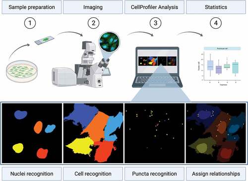
1. We provide the CellProfiler pipelines in which the CellProfiler-based detection of individual cells is based on the nucleus recognition based on the DAPI staining (Figure 1, Nuclei recognition), combined with the entire intracellular GFP (or AF488) fluorescence (Figure 1, Cell recognition). The detection of puncta (GFP-WIPI1, SQSTM1 or LDs) is based on the criteria size and fluorescence intensity over background (Figure 1, Puncta recognition), and recognized puncta are assigned to the corresponding cells (Figure 1, Assign relationships).

2. The CellProfiler pipeline “WIPI1_Airyscan.cpproj” was created for the analysis of GFP-WIPI1 puncta using Airyscan images and pipeline generation is summarized in Table S6.

3. The CellProfiler pipeline “WIPI1_LSM.cpproj” was created for analyzing single-plane image files (GFP-WIPI1, DAPI) obtained by confocal LSM. The generation of this pipeline is summarized in Table S7.

4. The CellProfiler pipeline “p62.cpproj” was prepared to analyze single-plane image files obtained by confocal LSM of endogenous SQSTM1 (AF488). The generation of this pipeline is summarized in Table S8.

5. The CellProfiler pipeline “LipidDroplets.cpproj” was prepared for the analysis of single-plane image files obtained by confocal LSM of endogenous SQSTM1 (AF488). The generation of this pipeline is summarized in Table S9.

6. These CellProfiler pipelines provided can be used as templates for analyzing your own image files. Alternatively, a new pipeline can be designed from scratch.

7. As a guide, the following describes how the CellProfiler pipeline “WIPI1_LSM.cpproj” was generated. Please refer to both Table S7 and in the corresponding Movie S1 for further detail.

8. Go to https://cellprofiler.org/releases and install the CellProfiler software for either Mac or Windows systems.

9. Download the provided CellProfiler pipeline “WIPI1_LSM.cpproj”.

10. To start, open the CellProfiler program and load the “WIPI1_LSM.cpproj” file by selecting “File”, “Open Project” from the dropdown menu. Select the “WIPI1_LSM.cpproj” file and click on “Open”. Confirm the loading of the pipeline by selecting the value “Yes” in the dialogue box.

11. Open the CellProfiler preferences and specify a default output folder in which your output files should be saved.

12. Before you adapt the “WIPI1_LSM.cpproj” pipeline for your analysis, upload your image files (or folder) to the “Image” module of CellProfiler using drag & drop.

13. Next, start adapting the “WIPI1_LSM.cpproj” pipeline so that CellProfiler can use this pipeline to recognize your images.

14. Rename the following using the “NamesAndTypes” module and refer to Table S7, steps 7 and 8. In step 7, replace “c1” with your file name or an abbreviation that contains enough information for the software to recognize all of the GFP single-channel image files that you want to analyze. In step 8, replace “WIPI1” if you want to analyze other punctate structures, e.g., “LC3”. Likewise, in step 13, replace “c2” with your file name or an abbreviation that contains enough information for the software to recognize all of the DAPI single-channel image files that you want to analyze. Then, refer to the Table S7, “Text input” column, and replace “WIPI1” with e.g., “LC3”. Then, always select e.g., “LC3” from all drop-down options. Also, tick e.g., “RelatedLC3puncta” in the “MeasureObjectSizeShape” module.

15. Depending on the content and structures of your images, use the pipeline settings “WIPI1_LSM.cpproj” as a template and optimize the numerical entries for the modules “IdentifyPrimaryObjects” and “IdentifySecondaryObjects”.

16. For adjustment purposes load a representative image into the “Images” module. Activate the “Test Mode” option by first pressing the “Start Test Mode” button and then the “Step” button. CellProfiler will now start analyzing the DAPI channel image using the first DAPI file in the list and the “IdentifyPrimaryObjects” module, and will preview the results in a pop-up window.

17. The pop-up window shows the original input image, the nuclei (in colors) CellProfiler detected in that particular image, the nuclei outlines applied to the original image, and the resulting values for that particular image. Importantly, xy-axis scaling is applied to each image based on the pixel size.

18. Nuclei outlines are coded as follows: green for accepted objects, magenta for discarded objects based on the diameter range, orange for discarded objects that touch the border of the image. Please note that cell nuclei are discarded in the pipelines provided if they are not fully represented in the original image. Corresponding cell parts are then filtered out.

19. Correct for inappropriate nuclei detection by changing the typical diameter range (Table S7, step 24, values in pixel) with reference to the xy-axis applied. We suggest starting with the following setting: (i) the range 50–500 for images with low resolution (e.g. 512 × 512 pixels), (ii) the range 300–1000 for images with high resolution (e.g. 3208 × 3208 pixels).

20. If necessary, also adjust here the “Threshold correction factor” (Table S7, step 31) to a lower value in order to make the threshold more lenient if too few nuclei are detected. Or choose a higher value to make the nuclei detection more stringent. We suggest starting with values within in the following ranges: (i) 0.4–1.0 for images with low resolution (e.g. 512 × 512 pixels), (ii) 0.285–0.5 for images with high resolution (e.g. 3208 × 3208 pixels).

21. After every value change introduced, press the “Step” button to rerun the “IdentifyPrimaryObjects” module again.

22. As soon as the adaptations that enable suitable nuclei detection have been made and no further changes are required, the “IdentifySecondaryObjects” module which recognizes the cell boundaries, is executed by pressing the “Step” button. Preview results are shown in an additional pop-up window.

23. The pop-up window now shows the original input image, the entire cell area (in colors) that CellProfiler has recognized, both outlines of the cell and the nuclei, as well as the result values. The outlines of the cell and nuclei are coded as follows: green for nuclei, magenta for cell boundaries.

24. Check the appropriate cell boundary detection. If necessary, adjust the “Threshold correction factor” value (Table S7, step 46). We suggest starting with the following setting ranges: (i) the range 0.1–0.8 for images with low resolution (e.g., 512 × 512 pixels), (ii) the range 0.2–0.6 for images with high resolution (e.g., 3208 × 3208 pixels).

25. As soon as the adjustments that enable suitable detection of cell boundaries have been made and no further changes are required, the “IdentifyPrimaryObjects” module, which recognizes GFP-WIPI1 puncta, is executed by pressing the “Step” button. Preview results are shown in an additional pop-up window.

26. The pop-up window shows the original input image, the puncta (in colors) recognized by CellProfiler in this particular image, the puncta outlines applied, and the result values for this particular image.

27. Puncta outlines are coded as follows: green for accepted objects, magenta for discarded objects based on the diameter range, orange for discarded objects that touch the border of the image.

28. Check adequate puncta recognition. If required, adjust the “Typical diameter of the objects” (Table S7, step 56). We suggest starting with the following setting ranges: (i) the range 2–170 for images with low resolution (e.g. 512 × 512 pixels), (ii) the range 4–100 for images with high resolution (e.g. 3208 × 3208 pixels). It should be noted that this range varies greatly depending on the resolution and marker structure used.

29. For the “Threshold correction factor” (Table S7, step 63) additional value changes may be required. Here, we suggest first to set the “lower bound on threshold” to 0 (Tab. S7, step 64) and starting with the following threshold correction factor setting ranges: (i) the range 1.0–3.2 for images with low resolution (e.g., 512 × 512 pixels), (ii) the range 1.6–3.3 for images with high resolution (e.g., 3208 × 3208 pixels).

30. Also set the “Size of adaptive window” value (Tab. S7, step 65) to a value greater than your maximum puncta diameter value. We suggest starting with the following setting ranges: (i) the range 5–250 for images with low resolution (e.g., 512 × 512 pixels), (ii) the range 45–120 for images with high resolution (e.g., 3208 × 3208 pixels). A good starting point here is to multiply the maximum puncta diameter value by 1.5 and use this value for the “Size of adaptive window”.

31. Next, starting over from step (15), use additional representative image files and also optimize the value for the “Lower bound on threshold” (Table S7, step 64), by using a lower value to exclude structures with weak fluorescence that may have been inappropriately recognized, and a higher value to exclude structures with strong fluorescence that have been inappropriately recognized as puncta. Here, we suggest starting with the following setting ranges: (i) the range 0.03–0.65 for images with low resolution (e.g., 512 × 512 pixels), (ii) the range 0.125–0.25 for images with high resolution (e.g., 3208 × 3208 pixels).

32. Finally, if puncta that are close to each are inappropriately recognized as an aggregate instead of being adequately separated, use the “Method to distinguish clumped objects” (Table S7, step 67). This was not the case for our applications, so this method was not used and the corresponding setting was set to “None” (Table S7, step 67). By instead selecting “Intensity” (Table S7, step 67) and choosing the “Yes” option for “Automatically calculate the size of smoothing filter for declumping”, a suitable puncta separation can be improved.

33. Now, all critical parameters for appropriate detection of nuclei, cell boundaries and puncta have been applied and adjusted so that CellProfiler can carry out the analysis using all image files and provide the output of interest (puncta per single cell and mean puncta area per single cell).

34. A difficult part, however, is to select an adaptation that enables puncta detection when such puncta change in both size and intensity due to different, e.g., compound, treatments. We therefore recommend adapting the pipeline based on further sample images obtained from different treatments.

35. After the pipeline has been optimized for your experiment, you can exit the test mode to run the CellProfiler analysis with the customized “WIPI1_LSM.cpproj” pipeline, by pressing the “Exit Test Mode” button and then the “Analyze Images” button to analyze all files.

36. During the analysis runs, the results appear in various pop-up windows. Finally, a folder called “PunctaCellsOverlay” is generated that contains image overlays and an additional folder called “PunctaCellsOverlayNumbers” is generated that contains image overlays with numbered cells. Further, the results are saved in separate tabular text files in the folder “CellProfilerResults”.

37. When the last CellProfiler run is complete, compare your original images with the image overlays applied by CellProfiler and assess the accuracy of nuclei, cell and puncta recognition. Depending on the accuracy of the recognition, add additional numerical changes if necessary.

Figure 1. Procedure for fluorescence-based GFP-WIPI1 image acquisition and analysis using CellProfiler. U2OS GFP-WIPI1 cells are prepared for fluorescence microscopy (Step 1, Sample preparation). Subsequently, images are acquired using fluorescence microscopy (Step 2, Imaging). Acquired image files are imported using the CellProfiler software (Step 3, CellProfiler Analysis), nuclei (Nuclei recognition), cell boundaries (Cell recognition) and GFP-WIPI1 puncta (Puncta recognition) detected and the corresponding puncta assigned to appropriate cells (Assign relationships). Finally, data are subjected to statistical analysis (Step 4, Statistics, generic bar graph displayed). This figure was created using BioRender.com with an imported U2OS GFP-WIPI1 Airyscan image as well as the associated CellProfiler-based detection of nuclei, cells and GFP-WIPI1 puncta.

Data processing

1. In the following we explain tabular text files that are derived from the CellProfiler GFP-WIPI1 puncta analysis using the pipeline provided here. If this pipeline is arranged or named differently, the following tabular text files change accordingly.

2. The tabular text files in our example are labeled as follows: “CellProfilerOutputImage”, “Cell Profiler Output Cells”, “CellProfiler Output Related WIPI1puncta”, “Cell Profiler Output Experiment”.

3. The tabular text file “CellProfilerOutputImage” contains information and data regarding the readouts per image given by CellProfiler, including number of cells per image (column header: “Count_Cells”), number of nuclei per image (column header: “Count_Nuclei”), number of related WIPI1 puncta per image (column header: “Count_RelatedWIPI1puncta”), the number of total WIPI1 puncta per image (column header: “Count_WIPI1puncta”), original file name given followed by an underscore and DAPI (column header: “FileName_DAPI”) and the image number assigned by CellProfiler (column header: “Image Number”).

4. The tabular text file “CellProfilerOutputCells” lists the following: image number given by CellProfiler (column header: “ImageNumber”), cell numbers whereby single cells are given a consecutive number (column header: “ObjectNumber”), the original file and path names (column headers: “FileName_DAPI”, “FileName_WIPI1”, “PathName_DAPI”, “PathName_WIPI1”), the number of puncta per cell (column header: “Children Related WIPI1puncta_Count”), the mean puncta area per cell (column header: “Mean_Related WIPI1 puncta _AreaShape_Area”), a duplicate of the values found in column Object Number (column header: “Number _Object_Number”).

5. The tabular text file “CellProfiler Output Related WIPI1puncta” contains image numbers given by CellProfiler (column header: “ImageNumber”), puncta numbers whereby single puncta are given a consecutive number (column header: “Object Number”), the original file and path names (column headers: “File Name _DAPI”, “File Name_WIPI1”, “PathName_DAPI”, “PathName_WIPI1”), the individual puncta area in pixels (column header: “Area Shape_Area”), a duplicate of the values found in column ObjectNumber (column header: “Number_Object_Number”), cell numbers whereby single cells are given a consecutive number (column header: “Parent_Cells”).

6. The tabular text file “CellProfilerOutputExperiment” contains the two columns Key and Value harboring the following keys “CellProfiler_Version”, “Channel Type_DAPI”, “Channel Type_WIPI1”, “Image Set_Zip_ Dictionary”, “Metadata_Tags”, “Pipeline _Pipeline”, “Run_Timestamp” with their respective values next to it.

7. These tabular text files (TXT files) derived from the CellProfiler analysis can be opened with Microsoft Excel and saved as XLSX files.

8. In the file “CellProfilerOutputCells”, the mean puncta area per cell in pixel was converted into the unit µm², based on the pixel size of the corresponding microscopy images.

9. For subsequent statistical calculations of puncta numbers and mean puncta area in single cells, the corresponding columns “Children Related WIPI1 puncta_Count” and “Mean_Related WIPI1 puncta _AreaShape_Area” are imported from the “Cell Profiler OutputCells” file into SPSS for subsequent data visualization and statistical analysis.

Inferential statistics

1. Using Microsoft Excel, the number of GFP-WIPI1 puncta-positive cells was expressed as mean percentages ± standard deviation and analyzed by two-tailed heteroscedastic Student’s t-testing. The data was displayed as bar graphs.

2. SPSS was used to apply non-parametric statistical methods in the analysis of single-cell data obtained with CellProfiler. The Shapiro-Wilk test was perfomed to test for normal distribution, and Kruskal-Wallis test with paired post hoc Dunn test and Bonferroni correction was used.

3. Briefly, to test for normal distribution, Shapiro-Wilk testing was carried out by selecting the options “Analyze”, “Descriptive Statistics” and “Explore … ”. A new window will open in which you can change the default settings as follows.

4. Select the list of the numbers of puncta per single cell as the “Dependent List” and the treatment (e.g., BafA1) as the “Factor List”. Switch to the “Plots … ” tab, deactivate the “Stem-and-leaf” option and activate the “Normality plots with tests” option. Save the settings by clicking the “Continue” and “OK” buttons one after the other.

5. An output file opens. In this outputfile, under “Tests of Normality” check whether the significance for the Shapiro-Wilk testing was <0.05 for all treatments. If so, data can be considered to be not normally distributed. Kruskal-Wallis tests with sequential Dunn-Bonferroni can be performed to test for significance by selecting the options “Analyze”, “Nonparametric Tests” and “Independent Samples … ”. Here, too, a new window opens in which you can change the default settings as follows.

6. Change to the tab “Fields” in the popup and select the list of counted puncta per cell as the “Test Fields” and the treatment (e.g., BafA1) as “Groups”. Change to the tab “Settings” and select “Customize tests”, “Kruskal-Wallis 1-way ANOVA (k samples)” and choose “All pairwise”. Accept the settings by closing the popup clicking on “Run” and check in the Output file whether the null hypothesis is accepted or rejected. Data were displayed as box plots with overlaid scatter plots.

7. P values <0.05 were taken to be statistically significant: *P < 0.05, **P < 0.01, ***P < 0.001.

Results and discussion

The phenotypic quantification of the fluorescent GFP-WIPI1 puncta numbers in single cells was carried out using the CellProfiler [25,26–34,35] model-based approach [38], with parameters that led to suitable image segmentation being adjusted manually.

In general, nuclei, cells and puncta were identified on the basis of characteristics based on shape size and fluorescence intensity (Figure 1). After segmentation of nuclei, cells and puncta, all of which are referred to as objects in CellProfiler, the objects were related to one another, which provided the number of puncta identified in single cells (Figure 1). Briefly, using the (1) “IdentifyPrimaryObjects” module of CellProfiler, cell nuclei were detected based on DAPI fluorescence by global Otsu thresholding, (2) based on the overall GFP fluorescence single cells were then detected with the “IdentifySecondaryObjects” module using using the “Watershed-Image method” with minimum cross-entropy thresholding, and (3) the “IdentifyPrimaryObjects” module with adaptive Otsu thresholding detected fluorescent puncta as foreground object based on pixel values (Figure 1, Table S7, Movie S1). Then, with the help of the “RelateObjects” module puncta were assigned to the corresponding cell, whereby identified cells were designated as parent and identified puncta as child objects (Table S7, Movie S1). Using a “MeasureObjectSizeShape” module, the puncta size was measured (Table S7, Movie S1). To visualize CellProfiler results, identified cells, nuclei and puncta were sketched with the “OverlayOutlines” and “DisplayDataOnImage” modules (Table S7 – S9, Movie S1, Fig. 2–4). CellProfiler data was then exported to spreadsheets for statistical analysis using Microsoft Excel or SPSS (Fig. 2–4).

Figure 2. GFP-WIPI1 puncta analysis by manual counting and CellProfiler-based detection. U2OS GFP-WIPI1 cells were either fed or starved and prepared for direct fluorescence microscopy (n = 3). (A) Stack image acquisition was conducted using Airyscan microscopy with the ZEISS LSM 800 and a representative image of U2OS GFP-WIPI1 cells in starved conditions is shown, displaying merged channels and z-projections (left panel: DAPI, GFP-WIPI1) or GFP-WIPI1 only (middle panel). 3D reconstruction of Airyscan acquired stack images was conducted, and typical GFP-WIPI1 puncta are shown in magnification (boxed in white) in the right panel. Scale bar: 10 µm. (B) Single-plane image acquisition of U2OS GFP-WIPI1 cells was conducted using Airyscan microscopy with the ZEISS LSM 800 and a representative image of U2OS GFP-WIPI1 cells in starved conditions is shown (left panel: DAPI, GFP-WIPI1), as well as subsequent CellProfiler analysis (middle panel: CellProfiler (CP) overlay). Magnified sections (1, 1’, 2, 2’) are shown in the right panels. Scale bar: 20 µm. (C) Using fluorescence microscopy, the number of GFP-WIPI1 puncta-positive cells was determined by manual counting (left panel: n = 3, 1539 fed cells, 1512 starved cells; two-tailed heteroscedastic Student’s t-testing, p-value: <0.001: ***). Next, based on the acquired single-plane Airyscan images the numbers of GFP-WIPI1 puncta in single cells was determined by manual counting (middle panel: n = 3; 147 fed cells, 198 starved cells). In comparison, acquired single-plane Airyscan images were subjected to CellProfiler analysis (right panel: n = 3; 131 fed cells, 231 starved cells). (D) Instead of Airyscan microscopy, single-plane image acquisition of U2OS GFP-WIPI1 cells in fed and starved conditions was also conducted using confocal LSM with the ZEISS LSM 800. Acquired confocal LSM images (left panel, DAPI, GFP-WIPI1) were subjected to CellProfiler analysis, and CellProfiler (CP) overlays are shown (middle panel) along with magnified sections (right panels; 1, 1’, 2, 2’). Scale bar: 20 µm. (E) Based on the acquired confocal LSM images the numbers (left panel) and sizes (right panel) of GFP-WIPI1 puncta in single cells was determined by manual counting (n = 4; 123 fed cells, 222 starved cells). (F) For comparison, CellProfiler-based analysis of the numbers (left panel) and sizes (right panel) of GFP-WIPI1 puncta in single cells is provided (n = 4; 89 fed cells, 221 starved cells). Statistics: Kruskal-Wallis with paired Dunn-Bonferroni correction, p-values: <0.001: ***.

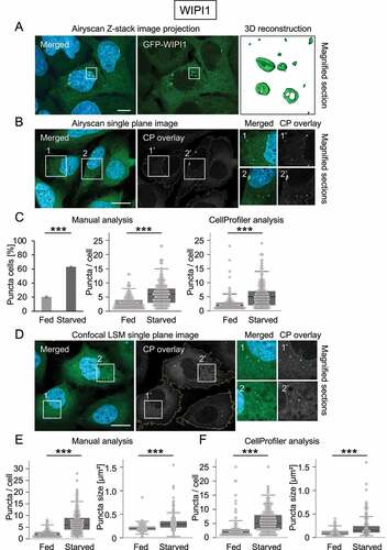
Figure 3. CellProfiler-based detection of endogenous SQSTM1 in U2OS cells. U2OS cells were either fed or starved, or treated with SAR405, BafA1 or torin 1, stained for nuclei (DAPI) and endogenous SQSTM1 (AF488, green), and single-plane images acquired using confocal LSM with the ZEISS LSM 800 (n = 4). Subsequently, a small-scale analysis of fed and starved cells was performed to compare manual versus CellProfiler-based assessments (A–C), or a larger analysis was conducted including all treatment conditions for CellProfiler-based assessments (D, E). (A) A representative image derived from starved conditions is shown (left panel, DAPI, SQSTM1), as well as the CellProfiler (CP) overlay (middle panel) along with magnified sections (right panels; 1, 1’, 2, 2’). Scale bar: 20 µm. (B, C) In the course of the small-scale analysis (n = 4; 26 fed cells, 28 starved cells), a subset of images derived from fed and starved conditions were analyzed with regard to the numbers (left panels) or sizes (right panels) of SQSTM1 puncta using manual counting (B) versus CellProfiler-based analysis (C). (D) Representative, magnified image sections of all treatments are provided (upper panels: merged image sections (DAPI, SQSTM1), lower panels: corresponding CellProfiler (CP) overlays). Scale bar: 10 µm. (E) Larger scale analysis of numbers (left panel) and sizes (right panel) of SQSTM1 puncta for all treatments was determined by CellProfiler-based analysis (n = 4; fed: 196 cells, starved: 215 cells, SAR405: 205 cells, BafA1: 212 cells, torin 1: 240 cells). Statistics: Kruskal-Wallis with paired Dunn-Bonferroni correction, p-values: <0.001: ***.

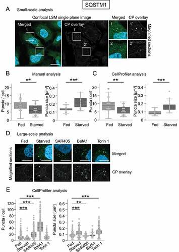
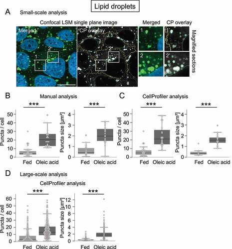
Figure 4. CellProfiler-based detection of LDs in U2OS cells. U2OS cells were either fed or treated with oleic acid, stained for nuclei (DAPI) and lipid droplets (LD) (LipidTOX Green), and single-plane images acquired using confocal LSM with the ZEISS LSM 800 (n = 4). Subsequently, a small-scale analysis was performed to compare manual versus CellProfiler-based assessments (A, B, C), or a larger analysis was conducted for CellProfiler-based assessments (D). (A) A representative image derived from oleic acid treatment is shown (left panel, DAPI, LDs), as well as the CellProfiler (CP) overlay (middle panel) along with magnified sections (right panels; 1, 1’, 2, 2’). Scale bar: 20 µm. (B, C) In the course of the small-scale analysis, a subset of images derived from fed and oleic acid conditions were analyzed with regard to the numbers (left panels) or sizes (right panels) of LipidTOX Green puncta using manual counting (B: n = 4, 30 fed cells, 22 cells treated with oleic acid) versus CellProfiler-based analysis (C: n = 4, 27 fed cells, 24 cells treated with oleic acid). Large-scale analysis including numbers (left panel) and sizes (right panel) of LipidTOX Green puncta was determined by CellProfiler-based analysis (n = 4; 267 fed cells, 426 cells treated with oleic acid). Statistics: Kruskal-Wallis with paired Dunn-Bonferroni correction, p-values: <0.001: ***.

Specifically, we have used the GFP-WIPI1 puncta formation assay [7,17,18,19] for confocal laser-scanning and Airyscan microscopy [36] and automated image analysis with CellProfiler (Figure 1, Figure 2, Movie S2) and provide a step-by-step protocol for creating the CellProfiler pipeline (Table S7, Movie S1). This CellProfiler pipeline can be employed as a template for ready-to-use analog analysis.

Despite the ease of use of the pipeline, there are a few caveats to be aware of. A high image quality is a prerequisite for the automated CellProfiler analysis and the first pipeline setups should be accompanied by an exemplary comparison of a small-scale analysis (e.g. 30 cells from n = 3) with CellProfiler and a manual image analysis (here with ImageJ, Fig. 2–4). Such setup procedure should then be extended to a larger analysis with more cells (here with appr. 100–300 cells from n = 3, Fig. 2–4). Once reliable CellProfiler results are available, it is recommended that several additional methods of analyzing autophagy and the autophagic flux, such as quantitative western blotting along with qPCR, be included to consider potential compensatory mechanisms [7].

As an example for such a procedure, we here first confirmed that GFP-WIPI1 stably expressed in a monoclonal U2OS cell line (U2OS-GFP-WIPI1) localized on autophagic membranes, visible as fluorescent puncta (Figure 2A, 2B, Movie S2), as previously described [7,17,18,19,21,22]. GFP-WIPI1 puncta were detectable in approximately 20% of cells in fed conditions, and in starvation-induced autophagy the number of GFP-WIPI1 puncta-positive cells significantly increased (Figure 2C, left panel). Hence experimental settings confirmed previous reports of the use of GFP-WIPI1 as a suitable marker for autophagy [7,17,18,19,21,22]. Next, we acquired Airyscan images of U2OS-GFP-WIPI1 cells and, using the identical set of images, we assessed the number of GFP-WIPI1 puncta per single cell manually (Figure 2C, middle panel) or alternatively using an automated CellProfiler-based analysis (Figure 2C, right panel). We extended this approach by using confocal LSM (Figure 2D), followed by comparative manual and automated analysis of both the number and the mean size of GFP-WIPI1 puncta per single cell (Figure 2E, 2F) Satisfactorily comparable results were obtained which confirmed a significant increase of autophagic puncta both in number and size under starvation conditions [7,39,40].

We also show that the CellProfiler pipelines created here for analogous evaluations of the autophagy receptor SQSTM1 or LDs lead to appropriate image segmentation under different treatment conditions (Fig. 3, 4). In this context, manual and CellProfiler-based assessments provided comparable results (Fig. 3, 4), and supported the notion that the number of SQSTM1 puncta decreases as their size increases under starvation (Figure 3), and that LDs increase both in number and size in the presence of oleic acid [41] (Figure 4). While employing further compounds for SQSTM1 puncta assessments in a larger CellProfiler-based analysis including 100–200 cells, we further confirmed that (i) due to inhibition of PIK3C3/VPS34 with SAR405 [42], SQSTM1 puncta numbers increased while their size decreased, (ii) due to BafA1-mediated inhibition of lysosomal acidification [43,44], SQSTM1 puncta numbers increased due to a block in the autophagic flux, and (iii) SQSTM1 puncta size increased upon autophagy stimulation with torin 1 [45]-mediated MTOR inhibition (Figure 3E). It is noteworthy that the exemplary analysis shown here for protocol purposes requires a further quantitative extension, such as the implementation of automated imaging in a multi-well format, e.g., with the LSM 800 used in this study or automated imaging stations [19] as part of hypothesis-driven approaches.

In summary, we show that CellProfiler-based subcellular recognition of GFP-WIPI1 is a reliable autophagy method for automated and unbiased approaches, and that this approach can easily be adapted for analog procedures, e.g., for the use of images with puncta referring to labeled SQSTM1 [46] or LDs [47]. The CellProfiler pipelines provided here can be downloaded and used directly, or used as a guide to design alternative or new pipelines for CellProfiler-based autophagy assessments [48,49].

Acknowledgments

T.P.-C. is funded by the Deutsche Forschungsgemeinschaft (DFG, German Research Foundation) under Germany’s Excellence Strategy Project-ID 390900677 – EXC 2180 (project 10076-1), the DFG Project-ID 314905040 – TRR 209 (project B02), the DFG Project-ID 323732846 – FOR 2625 (project 1), the DFG Project-ID 259130777 – SFB 1177 (project E03), the DFG Project-ID 327043846 – GRK 2364 (project 11), and by the DRIVE consortium, which is supported Marie Skłodowska-Curie ETN grant under the European Union’s Horizon 2020 Research and Innovation Programme (Grant Agreement No 765912).

Disclosure statement

No potential conflicts of interest was reported by the authors.

Supplementary material

Supplemental data for this article can be accessed online at https://doi.org/10.1080/15548627.2022.2065617

Additional information

Funding

This work was supported by the H2020 Marie Skłodowska-Curie Actions 765912 - ESR8 [765912]; DFG [EXC 2180 – 390900677]; DFG [314905040]; DFG [323732846]; DFG [259130777]; DFG [327043846].

References

- Ohsumi Y. Historical landmarks of autophagy research. Cell Res. 2014;24(1):9–23.
- Gomez-Sanchez R, Tooze SA, Reggiori F. Membrane supply and remodeling during autophagosome biogenesis. Curr Opin Cell Biol. 2021;71:112–119.
- Melia TJ, Lystad AH, Simonsen A. Autophagosome biogenesis: from membrane growth to closure. J Cell Biol. 2020;219(6):e202002085.
- Dikic I, Elazar Z. Mechanism and medical implications of mammalian autophagy. Nat Rev Mol Cell Biol. 2018;19(6):349–364.
- Mizushima N, Levine B. Autophagy In Human Diseases. N Engl J Med. 2020;383(16):1564–1576.
- Mizushima N, Murphy LO. Autophagy assays for biological discovery and therapeutic development. Trends Biochem Sci. 2020;45(12):1080–1093.
- Klionsky DJ, Abdel-Aziz AK, Abdelfatah S, et al. Guidelines for the use and interpretation of assays for monitoring autophagy. 4th edition)(1). Autophagy. 2021;17(1): 1–382
- Kabeya Y, Mizushima N, Ueno T et al. LC3, a mammalian homologue of yeast Apg8p, is localized in autophagosome membranes after processing. EMBO J. 2007;19(21):5720–5728.
- Kimura S, Noda T, Yoshimori T Dissection of the autophagosome maturation process by a novel reporter protein, tandem fluorescent-tagged LC3. Autophagy. 2007;3(5):452–460. DOI:10.4161/auto.4451
- Lamark T, Svenning S, Johansen T. Regulation of selective autophagy: the p62/SQSTM1 paradigm. Essays Biochem. 2017;61(6):609–624.
- Pankiv S, Clausen TH, Lamark T, et al. p62/SQSTM1 binds directly to Atg8/LC3 to facilitate degradation of ubiquitinated protein aggregates by autophagy. J Biol Chem. 2007;282(33):24131–24145.
- Roberts MA, Olzmann JA. Protein quality control and lipid droplet metabolism. Annu Rev Cell Dev Biol. 2020;36:115–139.
- Schepers J, Behl C. Lipid droplets and autophagy-links and regulations from yeast to humans. J Cell Biochem. 2021;122(6):602–611.
- Kirkin V. History of the selective autophagy research: how did it begin and where does it stand today? J Mol Biol. 2020;432(1):3–27.
- Lamark T, Johansen T. Mechanisms of selective autophagy. Annu Rev Cell Dev Biol. 2021;37:143–169.
- Stolz A, Ernst A, Dikic I. Cargo recognition and trafficking in selective autophagy. Nat Cell Biol. 2014;16(6):495–501.
- Mueller AJ, Proikas-Cezanne T. Automated detection of autophagy response using single cell-based microscopy assays. Methods Mol Biol. 2019;1880:429–445.
- Proikas-Cezanne T, Ruckerbauer S, Stierhof YD, et al. Human WIPI-1 puncta-formation: a novel assay to assess mammalian autophagy. FEBS Lett. 2007;581(18):3396–3404.
- Thost AK, Donnes P, Kohlbacher O, et al. Fluorescence-based imaging of autophagy progression by human WIPI protein detection. Methods. 2015;75:69–78.
- Proikas-Cezanne T, Takacs Z, Donnes P, et al. WIPI proteins: essential PtdIns3P effectors at the nascent autophagosome. J Cell Sci. 2015;128(2):207–217.
- Proikas-Cezanne T, Waddell S, Gaugel A, et al. WIPI-1alpha (WIPI49), a member of the novel 7-bladed WIPI protein family, is aberrantly expressed in human cancer and is linked to starvation-induced autophagy. Oncogene. 2004;23(58):9314–9325.
- Bakula D, Muller AJ, Zuleger T, et al. WIPI3 and WIPI4 beta-propellers are scaffolds for LKB1-AMPK-TSC signalling circuits in the control of autophagy. Nat Commun. 2017;8:15637.
- Dooley HC, Wilson MI, Tooze SA. WIPI2B links PtdIns3P to LC3 lipidation through binding ATG16L1. Autophagy. 2015;11(1):190–191.
- Dooley HC, Razi M, Polson HE, et al. WIPI2 links LC3 conjugation with PI3P, autophagosome formation, and pathogen clearance by recruiting Atg12-5-16L1. Mol Cell. 2014;55(2):238–252.
- Dobson ETA, Cimini B, Klemm AH, et al. ImageJ and CellProfiler: complements in open-source bioimage analysis. Curr Protoc. 2021;1(5): e89
- McQuin C, Goodman A, Chernyshev V, et al. CellProfiler 3.0: next-generation image processing for biology. PLoS Biol. 2018;16(7):e2005970.
- Dao D, Fraser AN, Hung J, et al. CellProfiler analyst: interactive data exploration, analysis and classification of large biological image sets. Bioinformatics. 2016;32(20):3210–3212.
- Bray MA, Carpenter AE. CellProfiler tracer: exploring and validating high-throughput, time-lapse microscopy image data. BMC Bioinformatics. 2015;16:368.
- Stoter M, Niederlein A, Barsacchi R, et al. CellProfiler and KNIME: open source tools for high content screening. Methods Mol Biol. 2013;986:105–122.
- Kamentsky L, Jones TR, Fraser A, et al. Improved structure, function and compatibility for CellProfiler: modular high-throughput image analysis software. Bioinformatics. 2011;27(8):1179–1180.
- Vokes MS, Carpenter AE. Using CellProfiler for automatic identification and measurement of biological objects in images. Curr Protoc Mol Biol. 2008;Chapter 14:Unit 14.17.
- Jones TR, Kang IH, Wheeler DB, et al. CellProfiler analyst: data exploration and analysis software for complex image-based screens. BMC Bioinformatics. 2008;9:482.
- Lamprecht MR, Sabatini DM, Carpenter AE. CellProfiler: free, versatile software for automated biological image analysis. Biotechniques. 2007;42(1):71–75.
- Carpenter AE, Jones TR, Lamprecht MR, et al. CellProfiler: image analysis software for identifying and quantifying cell phenotypes. Genome Biol. 2006;7(10):R100.
- Stoter M, Janosch A, Barsacchi R, et al. CellProfiler and KNIME: open-source tools for high-content screening. Methods Mol Biol. 2019;1953:43–60.
- Scipioni L, Lanzano L, Diaspro A, et al. Comprehensive correlation analysis for super-resolution dynamic fingerprinting of cellular compartments using the zeiss airyscan detector. Nat Commun. 2018;9(1):5120.
- Grotemeier A, Alers S, Pfisterer SG, et al. AMPK-independent induction of autophagy by cytosolic Ca2+ increase. Cell Signal. 2010;22(6):914–925.
- Caicedo JC, Cooper S, Heigwer F, et al. Data-analysis strategies for image-based cell profiling. Nat Methods. 2017;14(9):849–863.
- Jin M, Klionsky DJ. Regulation of autophagy: modulation of the size and number of autophagosomes. FEBS Lett. 2014;588(15):2457–2463.
- Munafo DB, Colombo MI. A novel assay to study autophagy: regulation of autophagosome vacuole size by amino acid deprivation. J Cell Sci. 2001;114(Pt 20):3619–3629.
- Pol A, Luetterforst R, Lindsay M, et al. A caveolin dominant negative mutant associates with lipid bodies and induces intracellular cholesterol imbalance. J Cell Biol. 2001;152(5):1057–1070.
- Ronan B, Flamand O, Vescovi L, et al. A highly potent and selective Vps34 inhibitor alters vesicle trafficking and autophagy. Nat Chem Biol. 2014;10(12):1013–1019.
- Klionsky DJ, Elazar Z, Seglen PO, et al. Does bafilomycin A1 block the fusion of autophagosomes with lysosomes? Autophagy. 2008;4(7):849–850.
- Yamamoto A, Tagawa Y, Yoshimori T, et al. Bafilomycin A1 prevents maturation of autophagic vacuoles by inhibiting fusion between autophagosomes and lysosomes in rat hepatoma cell line, H-4-II-E cells. Cell Struct Funct. 1998;23(1):33–42.
- Liu Q, Chang JW, Wang J, et al. Discovery of 1-(4-(4-propionylpiperazin-1-yl)-3-(trifluoromethyl)phenyl)-9-(quinolin-3-yl)benz o[h][1,6]naphthyridin-2(1H)-one as a highly potent, selective mammalian target of rapamycin (mTOR) inhibitor for the treatment of cancer. J Med Chem. 2010;53(19):7146–7155.
- Muralidharan C, Conteh AM, Marasco MR, et al. Pancreatic beta cell autophagy is impaired in type 1 diabetes. Diabetologia. 2021;64(4):865–877.
- Adomshick V, Pu Y, Veiga-Lopez A. Automated lipid droplet quantification system for phenotypic analysis of adipocytes using CellProfiler. Toxicol Mech Methods. 2020;30(5):378–387.
- Arias-Fuenzalida J, Jarazo J, Walter J, et al. Automated high-throughput high-content autophagy and mitophagy analysis platform. Sci Rep. 2019;9(1):9455
- Kolla L, Heo DS, Rosenberg DP, et al. High content screen for identifying small-molecule LC3B-localization modulators in a renal cancer cell line. Sci Data. 2018;5:180116