Performance of data-based models for early detection of damage in concrete dams

Abstract

A failure of a massive concrete dam could cause catastrophic consequences. The purpose of monitoring is to detect anomalies and damage at an early stage to prevent failure. Data-based models for anomaly detection are based on the hypothesis that the behaviour of an undamaged dam will follow an expected pattern, and deviation from this pattern is an indication of damage. In this study, simulations were used to create time series for an undamaged dam and three different damage scenarios at three different locations in the dam body. Three common data-based models were used to predict a dams crest displacements, both on the generated artificial data and the corresponding measurements from the dam. Prediction bands for future measurements were created, and the ten time-series were used to test the ability to detect damage. All models could detect instantaneous damage but struggle to detect progressive damage; the Neural network outperforms the two regression models. The choice of the mathematically optimal threshold limit leads to a large number of false alerts. Requiring three consecutive values outside the threshold before an alert is issued, increases the possibility to receive an early alert compared to the standard approach where observations are classified individually.

Keywords:

• Dam safety
• concrete dam
• data analysis
• monitoring
• statistical models
• anomaly detection
• false alarms

1. Introduction

A failure of a massive concrete dam could cause catastrophic consequences. Luckily, dam failures are rare, and the statistics of dam failure indicate that dam failure is a decreasing problem (Nordström, Malm, Johansson, Ligier, & Øyvind, 2015). The risk of failure is most significant for newly built dams. Of the failed dams, 25% failed as a result of the first impoundment and another 25% within the first five years (Nordström et al., 2015). The reduced cost and advances in sensor technology have meant that an increasing number of dams are monitored, and more sensors are placed on a typical individual dam. However, the collected data must be analyzed and evaluated from a dam safety perspective. There are examples of dams with automatic monitoring systems; whose failure was not preceded with a warning (Mata, Schclar Leitão, Tavares De Castro, & Sá Da Costa, 2014). The purpose of dam monitoring is to detect anomalies and damage at an early stage so that appropriate measures can be taken. In ICOLD’s bulletin on dam monitoring, the terms alarm and alert are used, where alarms are linked to a detected dangerous behaviour and alerts to unexpected behaviour (ICOLD’s Committee on Dam Surveillance, 2016). Therefore, an alarm implies an immediate risk of a dam breach and should be followed by direct action. An alert instead indicates damage and can usually be managed on a longer-term.

The detection of damage requires knowledge of the failure mechanism and the corresponding behaviour of the dam, and is thus, limited to the engineer’s ability to identify potential failure scenarios. Due to the rare occurrence, the exact failure-progression for a concrete dam is not well-documented. The early-age failures likely differ from the failure caused by wear-out, expected for technical components approaching its technical life span. There are indications that wear-out failure occurs progressively due to progressive deterioration and damage (Hariri-Ardebili & Saouma, 2015; Krounis, Johansson, & Larsson, 2015; Mata et al., 2014; Oliveira & Faria, 2006). An alternative approach is based on a hypothesis that the behaviour of an undamaged dam will follow an expected pattern, and a deviation from this pattern is an indication of damage. With this approach, each new measurement point is categorized as expected or unexpected. In order to do this classification, a suitable criterion must be defined. As each dam is more or less a unique structure, the behaviour of a dam must be determined on a case to case basis. This has led to the emergence of data-based models that are trained on previous measurements to predict the future behaviour of a dam.

The purpose of these types of models is to detect anomalies and damage already at an early stage. However, this feature of the models is seldom studied. The most common approach is to define warning limits using a prediction interval for future measurement values. In words, such an interval has the boundaries, prediction ± factor * standard error. This approach is recommended by SwissCOLD (2003) and ICOLD’s Committee on Dam Surveillance (2016) and used by for example by (Cheng & Zheng, 2013; Gamse & Oberguggenberger, 2016; Kao & Loh, 2013; Li, Wang, & Liu, 2013, Li et al., 2019; Loh, Chen, & Hsu, 2011; Salazar, Toledo, González, & Oñate, 2017). With this approach, each new observation is evaluated individually, and if the value is outside the prediction interval, an alert is issued. An example of more advanced categorizations is presented by Nguyen and Goulet (2018). One reason why the ability to categorize is rarely examined may be the lack of data with a clear distinction between damaged and undamaged. For natural reasons, such data with a distinct time point for damage initiation is difficult to obtain from measurements on real dams. To overcome this, simulations can be used to create data from a damaged and undamaged dam (Jung, Berges, Garrett, & Poczos, 2015; Mata et al., 2014; Salazar, Toledo, et al., 2017; Sevieri, Andreini, De Falco, & Matthies, 2019; Tatin, Briffaut, Dufour, Simon, & Fabre, 2015).

In this article, data-based methods are evaluated based on their performance to detect damage. Finite element (FE) simulations are used to created time-series data of the crest displacement of a concrete dam with and without damage. Two regression models; Hydrostatic seasonal time (HST) and Hydrostatic thermal time (HTT); and neural network are trained on the data. The trained models were tasked with classifying the time-series data as undamaged and damaged. Receiver operating characteristic (ROC) curves are used to evaluate their performance as classifiers.

2. Data and data creation

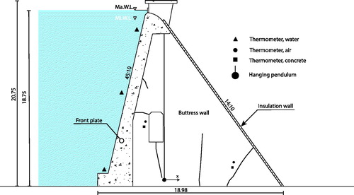
The research in this article was performed as a case study, where a 20 m high buttress dam in northern Sweden was used as the studied object. The dimension of the monolith and the position of all sensors are shown in Figure 1, also showing the main cracks in the monolith. This crack pattern includes three of the four crack types typically observed on buttress dams in Sweden; inclined cracks from the front plate that have propagated in the buttress toward the foundation; inclined cracks that have propagated from the inspection passage toward the front plate; and vertical cracks originating from the foundation, see Malm (2009) and Malm and Ansell (2011).

Figure 1. Sketch of the buttress dam used as a case study, and the location of sensors.

2.1. Measurements from the dam

The monitoring sensors that were installed on the dam in 2012 include; crack width measurements, hanging pendulum, extensometers, and temperature gauges. The hanging pendulum is recorded automatically with a laser of type Geokon BGK 6850A (Geokon, 2015). The top of the pendulum is attached under the bridge on the dam, and the laser is positioned 3.5 meters under the floor of the gallery. The bottom of the pendulum consists of a weight immersed in a container of liquid, that damps out small oscillations. The pendulum measures the crest displacements of the dam in two directions. In this study, data in the x-direction is used where positive and negative changes correspond to a movement of the crest in the upstream and downstream direction, respectively. The temperature is measured at seven positions at the monolith with sensors of the type Geosense Multipoint thermistor string (Geosense, 2017) with the following thermometers:

• One thermometer measures the air temperature outside the dam.

• Two thermometers measure the air temperature in the dam enclosed area between the front plate and the insulating wall

• Two thermometers are placed in the dam body and measures the concrete temperature.

• Three thermometers measure the water temperature at the depth 3, 13 and 23 m under the maximum water level.

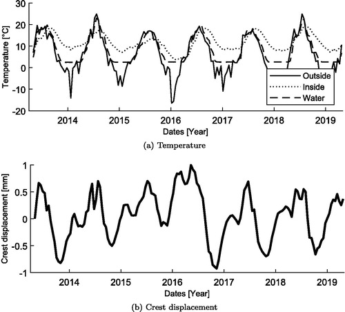
Within this project, measurement data from May 2012 to April 2019 have been used. The data was sampled hourly and was in this study downsampled to two-week intervals using the average value. Measured temperatures and crest displacements are shown in Figure 2.

Figure 2. Water and air temperatures and crest displacement from the studied dam. (a) Temperature., (b) Crest displacement.

2.2. Creation of data of crest displacements

The generation of data corresponding to the dam was done using simulations of the dams seasonal behaviour. The behaviour of the dam was simulated using temperature data measured at the dam for the period 2012–2019. Results from this simulation were used to compare the performance of the data-based models on measurements and simulations from the same period. Artificial data was created from using temperature data for the period between 1995 and 2013. First, the behaviour of the undamaged dam was simulated, and after that, nine simulations were performed with different types of damage initiated in the models. The simulations were performed as an uncoupled thermal-structural simulation where, in the first step, the temperature distribution in the concrete was calculated. The resulting temperature field was used as input to the mechanical model, and the strains and corresponding displacements from temperature variation were calculated. To mimic the measurement data, displacements corresponding to the hanging pendulum was extracted from the results. The model used for the simulations includes the dam and part of the surrounding rock, see Figure 3.

Figure 3. The FE-model and discretization used for the simulations. The three locations of damage, Front plate, Buttress, and Cracks are highlighted, and the application of the inside, T_I, outside, T_A and water T_W temperatures; and the insulation (i), air (a), and water (w), Robin boundaries are marked.

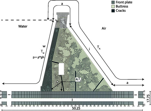
All numerical analyses were performed with Abaqus (Dassault Systemes, 2017), version 2017 with the standard implicit solver. One buttress with rock is modelled in 3D with 8-node linear brick elements with reduced integration and hourglass control (element DC3D8 and C3D8R in Abaqus). The average element size is 0.3 m for the dam. The rock was included in the model with the length 50.25 m in the upstream–downstream direction, the width 8 m in the direction perpendicular to the cross-section of the dam, and the height 17.75 m. The elements for the rock matches the dam at the contact surface from where the size gradually increases towards the boundary of the model. The simulation was performed in two steps, for temperature and static equilibrium, with a one-way coupling where the temperature was applied as a field in the static model.

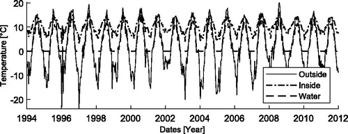
In the temperature model, an adiabatic boundary condition was applied to all rock surfaces except for the top. The top of the rock and the dam was divided into four surfaces; outside, inside, water and insulation. Figure 2(a) shows the temperatures used for simulation of the period 2012–2019. The measurements in the reservoir have shown that the water temperature is more or less constant over the depth and just above freezing temperature during the winter. Therefore, the water temperature has been assumed to be constant over the depth, and the measurements from the thermometer located 3 m under the water surface were used as the temperature for all surfaces in contact with water. For the period 1995–2012, hourly recordings of air temperature from the Swedish meteorological and hydrological institute (SMHI, 2019), taken at a weather station located approximately 20 km south-east of the dam (in the downstream direction) was used. The data of air temperature was used to create an approximation of the water temperature and the temperature in the enclosed area between the dam and insulation wall. For each time, the water temperature was taken as the greatest value of 0 °C and 80% of air temperature. The temperature inside the insulation wall was assumed to follow the air temperatures seasonal behaviour with the mean value 10 °C and amplitude of 30% of the air temperature. Figure 4 shows the three temperature time series. On each surface, the corresponding temperature was applied as a Robin boundary condition, as shown in Figure 3. A transient temperature simulation was performed for an 18 year-long period, starting from January 1995, using a two-week-long time-step. The length of the time step was chosen based on recommendations from Bühlmann, Vetsch, and Boes (2015) and Svensen (2016).

Figure 4. Air temperature outside and in the enclosure between the dam and the insulation wall, and water temperature.

In the static model, the boundary condition was applied to the rock by prohibiting displacements perpendicular to each side at all outer boundaries of the rock, except the top surface, see Figure 3. Based on previous studies from the same dam (Hellgren, Malm, & Nordström, 2019), a tie constraint was used in the interface between the dam and the foundation. For the concrete and the rock, linear material models were used, with the properties for the simulations presented in Table 1. The material properties used are based on previous reports were the elastic modulus, and the expansion coefficient of the concrete was calibrated to increase the agreement between the FE-model and the measurements (Hellgren, Malm, & Nordström, 2019), and the values used for the heat transfer coefficients are identical as those used by Malm, Hassanzadeh, and Hellgren (2017). The static simulations were performed in four steps, in the first step the dead load was applied, after that the hydrostatic pressure corresponding to the maximum water level was applied on the upstream part of the rock and dam, that water level was held constant during the succeeding steps. No uplift pressure in the dam-rock interface was included. Before the start of the full simulation, the first year of temperature variation was simulated three times to set the initial conditions in the dam.

Table 1. Material properties used for the simulations.

	Concrete	Rock	Unit
Density	2300	2300	kg/m^3
Elastic modulus	21.7	30.0	GPa
Poisson s ratio	0.2	0.2	–
Conductivity	1.7	1.7	W/mK
Specific heat	1000	1000	J/K
Expansion	10.6	8.3	$*{10}^6$ 1/K
Reference temperature	0	0	${}^{°}$ C
filmCoeff water	500	500	W/m^2/K
filmCoeff air	13	13	W/m^2/K
filmCoeff insulation	1	–	W/m^2/K

2.2.1. Damage

To simulate damage, three locations of damage in the dam and three scenarios were used, similar to Salazar, Toledo, et al. (2017). The first two locations were to introduce damage in either the whole front plate or the whole buttress. The third location was to introduce damage only in cracks corresponding to the crack pattern, as shown in Figure 3. 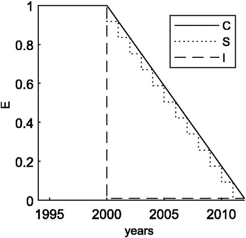The degradation was initiated as a reduction of elastic modulus, so that (1) $$E_d=d{E}_0$$(1) where d is a damage parameter, E₀ the initial elastic modulus and E_d the elastic modulus for the damaged part. The reduction in elastic modulus represents a decrease in stiffness for the structural part. For this, three simple damage time histories were used

• Scenario 1 – Continuous decrease

• Scenario 2 – Instantaneous decrease

• Scenario 3 – Seasonal decrease

In the continuous decrease scenario, the damage starts at a certain time and then the stiffness decrease linearly. This could represent a case where the damage may be caused by ageing or degradation mechanisms. For the instantaneous reduction scenario, all damage happens at one time. This could be the case if the dam is subjected to an accidental load or in other ways over-stressed so that significant damage occurs. The seasonal decline scenario is a mix between the other two approaches where the damage increases at distinct points every year. This is a fairly common type of scenario for this type of dam, where the damage successively increases each winter, see Malm and Ansell (2011). An illustration of the three approaches is shown in Figure 5.

Figure 5. The three used damage scenarios, C = Continuous, S = seasonal, and I = Instantaneous.

To generate pendulum data of the damaged dam, the three different scenarios were used for all three locations, resulting in a total of nine-time series with different types of damage. The final reduction of the E-modulus of the damaged part of the concrete was assumed to 50% in case the damage was defined the whole front plate or the whole buttress. This corresponds to induced micro-cracking in the elements, which is common in FE analyses of reinforced concrete when the crack spacing is smaller than the element length, see Malm (2009). When the damage was initiated in discrete cracks, a smeared approach was used where the E-modulus was reduced with 99% in the element with cracks. This corresponds to a fully developed macro-crack, see Malm (2016). Table 2 summarize the nine time-series of damage.

Table 2. Summary of the nine time-series of artificial data with different damaged scenarios.

Name	Structural part	Damage type	Max damage (%)
Bu-I	Buttress	Instantaneous	50
Bu-C	Buttress	Continuous	50
Bu-S	Buttress	Seasonal	50
Cr-I	Cracks	Instantaneous	99
Cr-C	Cracks	Continuous	99
Cr-S	Cracks	Seasonal	99
FP-I	Front plate	Instantaneous	50
FP-C	Front plate	Continuous	50
FP-S	Front plate	Seasonal	50

2.3. Simulation results

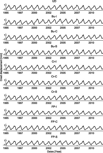
The results of the simulation are shown in Figure 6, and the data for the ten time-series and the temperatures are available for download (Hellgren, Malm, & Ansell, 2019). Both when individual time series are studied individually and when shown next to each other, it is difficult to observe any differences between damaged or undamaged cases.

Figure 6. Crest displacement measured at the studied dam. The first notation is the location of the damage (FP = Front plate, Bu = Buttress, and Cr = Cracks), and the second notation is the damage scenario (C = Continuous, S = seasonal, I = Instantaneous).

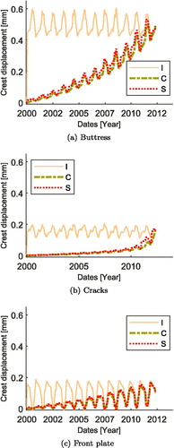
The difference between the undamaged and damaged data is shown in Figure 7(a–c). The approach with general damage in the buttress creates the largest difference, where the maximum difference is approximately 0.6 mm, 0.2 and 0.1 mm for the damage locations buttress, cracks and front plate, respectively.

Figure 7. Difference between the crest displacement for the undamaged and damaged dam. (C = Continuous, S = seasonal, I = Instantaneous). (a) Buttress, (b) Cracks, (c) Front plate.

3. Methods

3.1. Prediction models

There are many types of data-based models that can be used for dam behaviour analysis. Based on the review by Salazar, Morán, Toledo, and Oñate (2017), it is clear that different types of multilinear regression models, including HST, HTT, and neural networks, are the most frequently used model types. For this reason, HST, HTT and NN were selected. Below, a description of the implementation of these models is given.

3.1.1. Hydrostatic, seasonal, time

The HST model was first introduced by Willm and Beaujoint (1967) and has thereafter been a commonly used method for dam behaviour analysis for arch dams (Chouinard, Bennett, & Feknous, 1995; Fabre & Hueber, 2009; Tatin et al., 2018, 2015) roller-compacted concrete gravity dams (Dai, Gu, Zhao, & Qin, 2018), Earth fill dams (Fabre & Hueber, 2009; Zou, Bui, Xiao, & Doan, 2018), gravity dams (Léger & Seydou, 2009; Nedushan, 2002; Tatin et al., 2015) and buttress dams (De Sortis & Paoliani, 2007; Nedushan, 2002). HST is a multilinear regression model, where the variation in behavior of a dam is assumed to be a function of three parts according to Equation (2)(2) $$y_{\mathit{HST}}=F(H)+F(S)+F(t)$$(2) . (2) $$y_{\mathit{HST}}=F(H)+F(S)+F(t)$$(2)

Here H is the influence of hydrostatic pressure, S is a variable for the seasonal variation, and t is the irreversible changes that may occur over time. The model thus includes a function for each phenomenon that is considered to affect the global behaviour of the dam and is based on the hypothesis that these three variables are sufficient to explain the variation in the behaviour of a dam. Furthermore, the three variables are also assumed to be independent of each other, and the structural properties of the dam are assumed to remain constant over time. Usually, the hydrostatic pressure is modelled with a third- or fourth-degree polynomial. However, for the dam in this case study, where the water level only varies 0.5 m, a simple linear relation is assumed, (3) $$F(H)={\beta }_0+{\beta }_{1}h.$$(3)

Here, h is the relative water level related to the dam height H_dam and the reservoir level, WL, according to: (4) $$h=\frac{WL-BL}{H_{\mathit{dam}}},$$(4) where BL is the bottom level.

In HST, the temperature effects are modelled as a seasonal variation with the first terms in a periodic Fourier series, according to (5) $$F(S)={\beta }_5\hspace{0.17em}\text{sin}\hspace{0.17em}\left(\frac{2\pi t}{L}\right)+{\beta }_6\hspace{0.17em}\text{cos}\hspace{0.17em}\left(\frac{2\pi t}{L}\right)+{\beta }_7\hspace{0.17em}\text{sin}\hspace{0.17em}\left(\frac{5\pi t}{L}\right)+{\beta }_8\hspace{0.17em}\text{cos}\hspace{0.17em}\left(\frac{4\pi t}{L}\right)$$(5) where L = 52.18 if the time variable t has the unit weeks. This type of function neglects the actual temperature and predicts that it follows a seasonal pattern consisting of a full-year period and a half-year period. Some authors has successfully omitted the half year period for gravity dams in Nordic regions (Léger & Seydou, 2009), but since the response spectra of the measurements of the dam crest has a peak the half-year period (Hellgren, Malm, & Nordström, 2019), all terms where included in this study. The last effect is the irreversible changes over time. Here, the simplest form has been used where the relationship is assumed as completely linear, according to Equation (6)(6) $$F(t)={\beta }_{9}t$$(6) (6) $$F(t)={\beta }_{9}t$$(6)

3.1.2. Hydrostatic, thermal, time

In HTT, the seasonal behavior is replaced with a function that takes the actual temperature into account, (7) $$y_{\mathit{HTT}}=F(H)+F(T)+F(t)$$(7)

In this study, the outside air temperature T_A; inside air temperature T_I; and water temperature T_W was used. (8) $$F(T)={\beta }_5{T}_A+{\beta }_6{T}_I+{\beta }_7{T}_W$$(8)

3.1.3. Neural network

Neural networks (NN) are a group of algorithms that are based on the function of biological networks such as the human brain (Bowerman, O’Connell, & Koehler, 2005). Neural networks models are popular for dam behaviour analyses. In the review by Salazar, Morán, et al. (2017), 13 out of the 57 used models were NN. In short, a neural network consists of elements or nodes structured in several layers with connections between them. The typical neural network consists of three parts; input, core (hidden) and outputs. The nodes consist of two parts, a summing part, and an activation or transfer function. The summation part is the input to the node, where the weighted input from the signals to the nodes are summed. From there, the sum is sent to the transformation function and then out from the node. For a more comprehensive description, see for example Bowerman et al. (2005) or Hastie, Tibshirani, and Friedman (2009).

In this study, the training approach was adopted from Salazar, Toledo, Oñate, and Morán (2015), which is based on a combination of the works by Mata (2011) and Hastie et al. (2009). The training was performed using Matlabs’ statistical toolbox (The MathWorks Inc., 2018). For the training process, the Levenberg-Marquardt backpropagation learning rule algorithm was used (Marquardt, 1963). A three-layer NN was used with a hyperbolic transformation function, and the input variables were; water level, air and water temperature; time; season ($\text{sin}\hspace{0.17em}(2\pi t/L)$ and $\text{cos}\hspace{0.17em}(2\pi t/L)$). 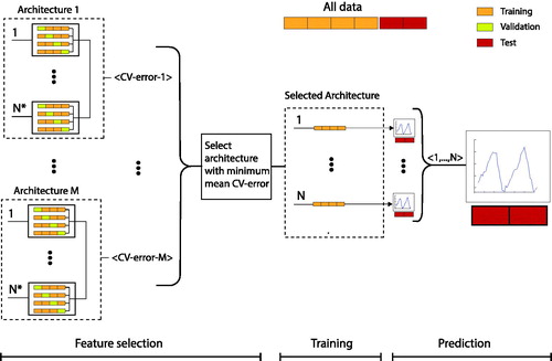The following sizes were used for the hidden layer, 3, 12, and 25. For each size of the network, three regularisation parameters were used, 0.1, 0.01, and 0.001. The training approach is illustrated in Figure 8. For each combination of parameters, 15 different random initiations of weights were tested. The combination with the lowest cross-validation mean square error was chosen as the final design. After that, the network with the chosen design was trained on the whole training set for 20 different initiations. The model was then assessed using the average of the predictions from the 20 models as the final prediction.

Figure 8. Illustration of the training approach where M = 9 designs (all combinations of 3, 12, and 25 nodes in the hidden layer and regularisation parameter 0.1, 0.01, and 0.001) were trained with N*=15 different random initiations of weights. The combination with the lowest cross-validation error was chosen. The chosen design was re-trained on the whole training set for N = 20 different initiations. The final prediction for the test set was the average of the predictions from the 20 models.

3.1.4. Measures of accuracy

As the measures of prediction accuracy, the determination coefficient R² and the normalized mean absolute average, NMAE was used. Here, the error is normalized with regards to the total amplitude of each series, $\max (y)-\min (y),$ so that the accuracy can be compared between measurements and simulations. (9) $$\text{NMAE}=\frac{\sum _{n=1}^N\left|y_n-{\widehat{y}}_n\right|}{\max (y)-\min (y)}$$(9) where ${\widehat{y}}_n,$ is a prediction of the response variable y_n at observation n of the total N observations. The determination coefficient R² is interpreted as the fraction of the variance in the dependent variable explained by the model: (10) $$R^2=1-\frac{\sum _{n=1}^N{\left(y_n-{\widehat{y}}_n\right)}^2}{\sum _{t=1}^N{\left(y_n-\overline{y}\right)}^2}$$(10) where $\overline{y}$ is the mean of y.

3.2. Alert

3.2.1. Setting alert limits

As mentioned in the introduction, the most common approach is to create warning limits using a prediction interval for future measurement values. In words, such an interval has the boundaries, prediction ± factor * standard error. This approach was also used in this article. The standard deviation of the residual on the test set, s, was used as an estimate for the standard error (11) $$s=\sqrt{\frac{1}{N-1}\sum _{n=1}^N{\left(y_n-{\widehat{y}}_n\right)}^2}$$(11)

The upper and lower limits of the prediction interval are calculated (12) $$\left[\widehat{y_n}+Ks,\widehat{y_n}-Ks\right]$$(12) where K is a factor often set as chosen quantile for a standard normal distribution. If a measured value falls outside these limits, the behaviour of the dam is categorised as unexpected, and an alert is issued. In addition to the standard approach, a method where three consecutive observations are outside the prediction interval before an alert is issued was tested.

3.3. Assessing alert limits

There are four possible outcomes for the classification, true-positive TP, false-positive FP, true-negative TN, and false-negative FN. A positive means that models indicate damage and a TP means that the model issues a warning and that damage has occurred on the dam. In this study, the following definitions were used.

TP – an alert is issued when evaluating a data point from the damaged time-series

FP – an alert is issued when evaluating a data point from the undamaged time-series

FN – no alert is issued when evaluating a data point from the damaged time-series

TN – no alert is issued when evaluating a data point from the undamaged time-series

The receiver operating characteristic (ROC) curve was used to evaluate the classification performance. In a ROC-curve, the true positive rate (TPR): (13) $$\text{TPR}=\frac{\text{TP}}{\text{TP}+\text{FN}},$$(13) is plotted against the false positive rate (FPR): (14) $$\text{FPR}=1-\text{TNR}=\frac{\text{FP}}{\text{FP}+\text{TN}}$$(14)

The threshold for an alert was varied by altering the factor K in Equation (12)(12) $$\left[\widehat{y_n}+Ks,\widehat{y_n}-Ks\right]$$(12) from 0 to 5 in steps of 0.1. The FPR was calculated on the undamaged data and the TPR for the nine time-series with damaged data. C-Statistic was calculated for each model for the nine series of data. The C-Statistic is also known as the area under the curve (AUC) for the ROC and is a measure of goodness of fit for binary outcomes Hastie et al. (2009). A C-Statistic of 0.5 indicates a poor model where the model adds no predictive value compared to a random chance. In contrast, a C-Statistic value of 1.0 means that the model perfectly classifies the data. The Youden Index J was used to determine an optimal threshold. The Youden Index J is calculated as (15) $$J=\text{TPR}-\text{FPR},$$(15) and is a measure of the vertical distance from a point on the ROC-curve and the chance line. The index is defined for all points of a ROC-curve, and the maximum value of the index was used as a criterion for selecting the optimal threshold.

3.4. Outline of analysis and data division

For models fitted to data, the risk of overfitting is always present. It is therefore essential to assess the performance of a model on the data not used in the fitting process. The data should be divided into a training and a test set. The training set is used to train the model and update its properties while the performance of the model is assessed on the test set. Hence, the test set serves as independent data, that does not affect the models’ properties. Further, for selection between several models or several properties of one model, the training data should be divided into a training set a validation set. The validation set is, as the test set, a set of data not used directly for training. The training data set is used to train the models, the choices between different model parameters, and when to stop training are based on the models’ performance on the validation set.

Two sets of analysis were performed

1. Comparison of the prediction models performance on real measurement data and artificial data.

2. Evaluation of the performance of the categorisation of the dam as undamaged or damaged.

Figure 9 shows the data division used in this article for the comparison between the prediction models performance on simulation. For the first set of analysis when the models’ performance on real measurement data and artificial data, the training set length was four years, and the test set two years. To test the sensitivity of the predictive accuracy on the simulation, a random error was added as white noise to the crest displacement from the simulation. Three levels of error were used, 0.1 mm, which is the measurement error for the hanging pendulum (Geokon, 2015), and five and ten per cent of the maximum amplitude.

Figure 9. Division of the data in training, validation, test and evaluation test.

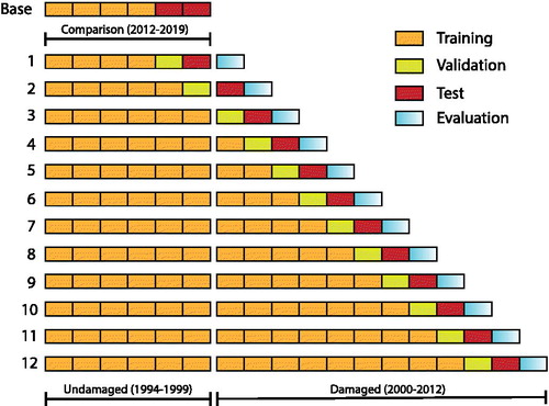
For the evaluation of the performance of the categorisation, the data was divided into four parts. The NN model was trained on the training set until the error on the validation set was minimised. The HST and HTT model was fitted using ordinary least squares on the data in the training set and validation set. Hence, since the linear regression models are fitted, the use of a validation set is obsolete and more data can be used for training. After that, the trained models were used to predict the data in the test set. The standard error of the residuals in the test set was calculated. This standard error was used to create the prediction interval for the evaluation set. The categorisation ability was thereafter assessed on the evaluation set. After that, a new year was added as the new evaluation set, and the process was repeated.

4. Results

4.1. Prediction accuracy on measurements and simulations

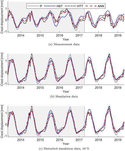
Figure 10 shows the three series of crest displacements from measurement, simulation and disturbed simulation together with the prediction from the models. The first four years are the training data, and the last two years are the test data. For the measurement data, all three models show good agreement with the measurement data, but NN and HTT outperform the HST model. This is obvious during year three, which was a cold year where the two models that include the temperature has significantly better accuracy than HST. For the two series of simulation, the HTT does not describe the behaviour of the dam. It is mainly the behaviour during the winters when the water temperature is zero that are incorrectly predicted. This is due to higher multicollinearity between the temperatures used in the simulation than the measured temperatures.

Figure 10. Crest displacement and prediction for training (year 0–4) and test (year 4–6). (a) Measurement data, (b) Simulation data, (c) Disturbed simulation data, 10%.

The best design for the NN was 3 neurons and regularization parameter 0.1 for the measurement and all simulations. Table 3 presents a comparison between the prediction results for the measurement data and the artificial data. The comparison shows that for all models, the use of simulation data leads to an overestimation of the prediction accuracy of the model compared to the prediction results for the data from the measurements. The table also shows the prediction performance for the simulated data with an introduced random error. For an error with the size of the measurement accuracy, the difference is small, and such an error has a small effect on the accuracy.

Table 3. Comparison of prediction accuracy for HST, HTT and NN for the measurements and simulations. The first row presents the performance of the models on data from the measurement. The second row shows the performance on data from the simulation, and row three to five presents the performance on data from the simulation with added white noise.

	Training, N = 104						Test, N = 53
	HST		HTT		NN		HST		HTT		NN
	R^2	NMEA	R^2	NMAE	R^2	NMAE	R^2	NMAE	R^2	NMAE	R^2	NMAE
Measurement	0.65	0.17	0.91	0.07	0.92	0.07	0.83	0.09	0.86	0.07	0.95	0.05
Simulation	0.94	0.06	0.92	0.07	0.96	0.06	0.97	0.04	0.93	0.07	0.97	0.05
Disturbed 1 mm	0.94	0.06	0.92	0.07	0.96	0.06	0.97	0.05	0.93	0.07	0.97	0.06
Disturbed 5%	0.93	0.06	0.91	0.07	0.95	0.06	0.97	0.05	0.93	0.07	0.97	0.05
Disturbed 10%	0.92	0.07	0.91	0.07	0.95	0.06	0.96	0.05	0.92	0.07	0.96	0.06

4.2. Length of data

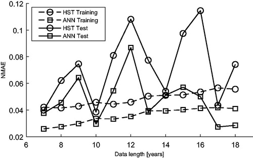
Figure 11 shows how the test and training NMAE evolves as the length of the data increases. As outlined in Figure 8, the test length is kept constant at one year while the extra data is added to the training set. Due to the problems with multicollinearity on the simulations for HTT, the model was excluded from further analysis. For all models, the difference between the standard error for the test set and training set differs significantly. In general, the two models have higher test error than training error. The training error continuously increases with additional data length while the test error behaves more randomly. For NN, there is a trend towards a reduced test error with increased data length, and the last two errors are lower than the corresponding training error. However, the test error fluctuates and sometimes increases as additional data is added.

Figure 11. Training and test error as a function of data length.

4.3. Alert limits

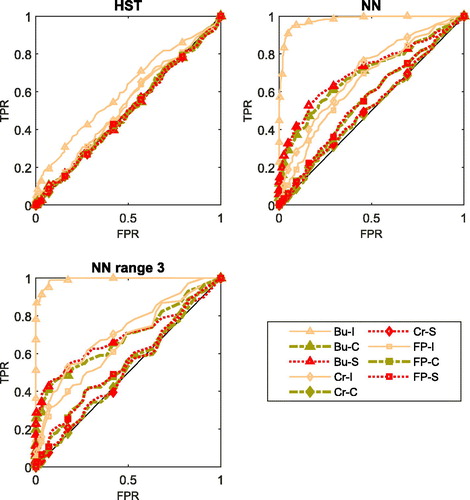
Figure 12 shows the ROC-curves for the categorisations of the different studied models. It is clear that the neural network performs better than HST.

Figure 12. ROC-curve for the four prediction models. The first notation is the location of the damage (FP = Front plate, Bu = Buttress, and Cr = Cracks), and the second notation is the damage scenario (C = Continuous, S = seasonal I = Instantaneous).

Table 4 presents the C-statistic and the threshold that has the maximum Youden index for the nine sets of simulated damage. Here it is seen that further improvement is achieved by requiring three values in a row outside the threshold before an alert is issued increases the performance further. There is a considerable variation between the various damage locations in how good the models are at alerting for damage. Best of all models in the time series perform with general damage to the wall with an instantaneous accident. The result shows that the models can detect instantaneous damage in the buttress to a greater extent compared to the others. On this series, the neural network performs very well, with C statistics of 0.98 and 0.99 for one and three observations, respectively. Overall, all models can detect that both instantaneous and progressive damage in the buttress has changed the dam behaviour. For damage in the front plate or due to cracks, it is only for the instantaneous damage that the models add predictive value. For slow progressive damage, the classification performs equally as chance. The table also shows the optimal K value, selected as the highest Youden index and the FPR for that value. The optimal K varies greatly between the different models and types of damage. For a majority of cases, K is below the 2.0, which is approximately equal to a 95% prediction band. When the K value is selected by the Youden index, the number of false positives is high. The lowest value of 8% is given by NN3 for instantaneous damage in the buttress, while the HST model for an instantaneous damage initiation in the front plate has a FPR of 59% and is even worse for the two progressive scenarios.

Table 4. Performance for the three models on the nine time-series. AUC, the K-factor with highest Young index and FPR for that factor. The first notation is the location of the damage (FP = Front plate, Bu = Buttress, and Cr = Cracks), and the second notation is the damage scenario (C = Continuous, S = Seasonal, I = Instantaneous).

	HST			NN			NN3
	AUC	K	FPR	AUC	K	FPR	AUC	K	FPR
Bu-I	0.61	1.85	0.20	0.98	2.18	0.07	0.99	1.09	0.08
Bu-C	0.50	2.50	0.05	0.70	1.17	0.30	0.69	1.01	0.09
Bu-S	0.50	2.30	0.08	0.71	1.41	0.21	0.69	1.01	0.09
Cr-I	0.52	0.77	0.59	0.70	0.85	0.43	0.72	0.77	0.18
Cr-C	0.50	0.48	0.73	0.51	1.41	0.21	0.52	0.08	0.82
Cr-S	0.49	1.65	0.25	0.52	1.61	0.16	0.52	0.08	0.82
FP-I	0.53	0.77	0.59	0.65	0.81	0.46	0.66	1.05	0.08
FP-C	0.50	0.52	0.69	0.55	0.77	0.47	0.55	0.56	0.28
FP-S	0.50	0.52	0.69	0.56	1.01	0.36	0.56	0.60	0.26

Table 5 shows the number of days it takes from the initiation of damage until the first alert if K is selected so that the number of permitted false alerts per year is 0, 1 and 2. The value 0 means that no false alerts are given during the entire period. The first rows show $K*,$ the values of K that fulfils that this. Compared to the optimal values presented in Table 4, these values of K are higher. A more generous acceptance for false alerts means that narrower intervals can be selected and that damage can be detected more quickly. This is seen in the number of weeks from damage initiation to the first alert. For the requirement of no false alert, the first true positive will be detected after a long time or never. If instead one false alert per year is permitted, that time is reduced significantly. For permission of maximum of two false alerts per year, all models correctly warn for damage within two years regardless of the rate of damage initiation and damage location. In cases of instantaneous damage in the buttress, all models issue an alert at the first possible instance. The NN model with three consecutive points outside the threshold also issues an alert within at the first possible instance for the cases with damage localisation through cracks in the monolith. However, it should be noted that the analysis here is based on bi-weekly values; so the first possible instance is two and six weeks for one and six weeks, respectively. For the case with instantaneous damage in the front plate, this model issues an alert within ten weeks.

Table 5. The first row shows the maximum allowed false-positive per year and the second row shows the corresponding value of K. The other rows show the number of weeks from the initial damage initiation until the first alert is issued for each damage scenario and location. The first notation is the location of the damage (FP = Front plate, Bu = Buttress, and Cr = Cracks), and the second notation is the damage scenario (C = Continuous, S = seasonal I = Instantaneous).

	HST			NN			NN range 3
	0
Max FP	3.79	1	2	0	1	2	0	1	2
$K*$	Weeks to first alert	2.62	2.38	3.71	2.54	2.18	2.18	1.41	1.05
Bu-I	18	2	2	18	2	2	6	6	6
Bu-C	230	88	88	230	88	88	268	28	28
Bu-S	230	88	88	230	88	18	266	28	28
Cr-I	Inf	18	18	230	18	18	28	20	10
Cr-C	230	88	88	Inf	88	78	278	120	28
Cr-S	230	88	88	Inf	88	78	278	120	28
FP-I	20	18	18	230	18	18	266	10	6
FP-C	Inf	88	88	230	88	78	268	120	28
FP-S	Inf	88	88	230	88	78	268	120	28

5. Discussion

Table 3 present R² for the prediction of measurements and simulations with HST, HTT and NN. These results can be compared to De Sortis and Paoliani (2007) who used a HST model on a total of thirteen monoliths from three buttress dams (Ancipa (15 years data), $R^2=0.98,0.95,0.96,0.97,0.97$); Sabbione (5 years) $R^2=0.96,0.96,0.95$); and Malga Bissina (9 years) $R^2=0.88,0.91,0.92,0.92,0.90$); Nedushan (2002) who predicted the crest displacement of a buttress dam with HST ($R^2=0.95$) and HTT ($R^2=0.96$). Compared to previous studies, the prediction in this study is in line with or slightly better than comparison from the literature. Hence, prediction accuracy should not be a limitation compared to other studies for the models used in this article.

Since its difficult to get data with from real dams with a clear division between undamaged and damage, it is common to evaluate these types of models on data created by simulations (Jung et al., 2015; Mata et al., 2014; Salazar, Toledo, et al., 2017; Tatin et al., 2015). This study shows some difference between the artificial and the real data. It is therefore unclear how applicable evaluation of models on artificial data is to judge their performance on real cases. The disadvantage of using artificial data compared to measured is that the reality is more complex than normally can be accounted for in a model. The studied dam is located in a cold climate, thereby factors such as ice, snow and solar radiation may also affect the dam’s behaviour. In addition, measurement errors are also a potential source of error. However, the simulation with added measurement error in the present study indicated that measuring accuracy shows only a small influence on the models’ accuracy. The performance on artificially generated data should be considered as an upper bound on the performance, and it difficult to evaluate how good a model is at detecting damage for a real dam. In cases where simulations are used to generate damage, theses simulations are also limited by the accuracy for simulation of damage and how well the types of damage that occur on a dam can be predicted. Despite the idealized simulation used in this study, most of the model show low ability to alert for progressive damage while instantaneous damage in larger areas is more easily detected. Hence, the results show that further development is needed especially to be able to capture progressive damage evolution which is expected to occur due to ageing and wear.

Salazar, Morán, et al. (2017) reviewed 57 studies from 41 articles presented at conferences and in scientific journals about dam behaviour models. Of the 41 articles, most studies use small validation sets. Although it is common knowledge that data should be divided into training and test sets to avoid overfitting and that the model’s performance should be evaluated on unseen data. In total, 20 out of 41 articles have completely omitted to divide the data and performed the training and evaluation on the complete data. The results clearly show that the test error, in general, is higher than the training error, and when models are evaluated and compared, this should be done on unseen data. Both the required length of data and the sampling frequency varies between different types of models, and it is difficult to establish any general guidelines. For dam behaviour analysis, this length has not been established. In the literature, the used data length varies from 1.5 to 25.5 years (Salazar, Morán, et al., 2017). Two recommendations are to use at least three (ICOLD’s Committee on Dam Surveillance, 2016), or five annual cycles (SwissCOLD, 2003). However, there are examples of when a data length of 10 years was required before the models were stable (De Sortis & Paoliani, 2007; Lombardi, Amberg, & Darbre, 2008). In the present study, no clear improvement in the NMAE is achieved when the data length increases from six to fourteen year. Instead, the error varies from year to year, and for the HST model, there is a trend towards an increased error as the data length increases. Hence, the results in this study do not support a distinct cutoff point, for which a sufficient data amount is achieved. The indications are instead that more data is better, but that the accuracy can decline during a single year due to random effects in the data. Similar results are presented by, for example, Salazar et al. (2015).

Although the primary purpose prediction models are to provide early indications of damage, few tests of that ability are presented in the literature, see for instance Cheng and Zheng (2013); Gamse and Oberguggenberger (2016); Kao and Loh (2013); Li et al. (2013, 2019); Loh et al. (2011); Salazar, Toledo, et al. (2017). One reason for this is that it is difficult to obtain data with a clear delimitation between a damaged and an undamaged dam. This study shows that although the models perform well, only certain types of damage occur where the models add classification value. This shows the benefit of continued research in the area, where even small improvements in prediction ability (R² and NMAE) can increase the ability to classify damaged compared to undamaged. Furthermore, it should be pointed out that although the most serious damage looks major in Figure 12 when compared to the undamaged dam, it is something that a human eye would find difficult to discern as damage, see Figure 6. Although the HST model has an almost equivalent prediction performance as the Neural network, it performed significantly worse as a classifier. This indicates that for models used with the purpose of setting alert thresholds, prediction accuracy is important, and it worth to lose some interpretability as a trade-off for extra predictability. Other machine learning models such as support vector machine and boosted regression trees may be better suited for this dam and perform even better the NN. However, the prediction ability is not the main bottleneck for the categorization. The novel approach of requiring three consecutive observations outside the prediction interval before an alert is issued improves the categorization. This is an indication of the usual method, where each measurement is evaluated one by one could be improved if a series of observations are categorized together. Here, more advanced categorization approaches from the field of change detection and concept drift should be tested.

In this article, the performance of data-based models is investigated. In reality, the data-based model in specific, and monitoring in general, should be a part of a broader condition assessment program that also includes, risk assessments, qualitative assessment of the condition and behaviour of the dam, checking and testing, and visual inspections. The results show the need to include several data points in the categorization. Other authors have demonstrated success in using methods that combines information from several sensors, for example, via a principal component analysis (PCA) (Chouinard et al., 1995; Jung et al., 2015; Mata et al., 2014; Yu, Wu, Bao, & Zhang, 2010). Such combination can be performed by combining information from several sensors of the same type, or by combining information from several types of global and local sensors such as relative displacements, movement of cracks and joints, rotations, the volume of seepage under the dam, water pressures in one analysis. Regardless of whether several subsequent observations or several measurements at the same time are included, the results in this article indicate that such methods could reduce the number of false alarms.

The Youden index weights all errors equally and does not considers that there may be different consequences for a false-negative or a false-positive. It is not only the trade-off between sensitivity and specificity that must be considered when setting the threshold value. The probability of the occurrence of damage must also be considered. If the appearance of positive events is rare, the model will mainly classify negative events. Hence, the prevalence of false-positive will be magnitudes greater than the prevalence of true positive events. As an example, a model with 100% sensitivity and 99% specificity that will categorize an observation every week during 20 years, a total of 1560 observations. During that period, a damage event will occur, and a TP will be registered. At the same time, and that about 15 FP alerts will be sent and that the probability of a real event occurring when an alert goes off is thus only 1/16 (6%). If the sensibility is decreased to 95%, the number of false-positive will increase to 78, meaning that the probability of real damage when a warning is issued is then decreased to 1/78 (1.4%). For a dam owner, it is therefore important to not set too narrow alert limits as that results in an unmanageable amount of false alert. On the other hand, zero-tolerance against false alerts delays the detection of real damage. The acceptance for false alerts is higher compared to false alarms, considering that an alarm indicates an immediate risk of a dam breach, and is typically followed by direct action. However, it is important that the number of false alerts is kept low, considering that there is a higher risk of negligence with an increasing number of false alerts. In the present study, the ability to detect damage has been studied using a typical Swedish buttress dam as a case study. The generality of these results is not known, and further studies should continue to test the data-based models performance on detecting damage in other dam-types, such as gravity dams, RCC gravity dams, and arch dams, etc.

6. Conclusions

Three prediction models have been used to predict crest movements of a Swedish concrete dam. For predictive ability, NN performs best, although the simpler regression models have adequate prediction ability. Comparison between measurement and artificial data shows that the models generally perform better on artificial data but that there are exceptions. All models have a better capability to detect instantaneous compared to progressive damage. However, the NN method shows some capability to detect progressive damage, at least if it occurs in rather large areas such as the whole buttress. Further research in this area is vital considering that for existing dams, ageing or wear cause progressive damage evolution rather than instantaneous.

Requiring three consecutive values outside the threshold before an alert is issued, increases the possibility to receive an early alert compared to the standard approach where observations are classified individually. This is an indication that more advanced categorization approaches based on the evolution of the time-series, using methods from the field of change detection and concept drift, should be tested in the future.

In general, the optimal threshold determined as the maximum Youden index is below the commonly used 2.0. However, the choice of the mathematically optimal limits leads to a large number of false alerts. If the limits are set so that false alerts are completely avoided, the detection of damage is significantly delayed. A more generous acceptance for false alerts means that narrower intervals can be selected and that damage can be detected more quickly.

Acknowledgements

The research presented was carried out as a part of” Swedish Hydropower Centre – SVC”. SVC has been established by the Swedish Energy Agency, Elforsk and Svenska Kraftnät together with Luleå University of Technology, KTH Royal Institute of Technology, Chalmers University of Technology and Uppsala University. www.svc.nu.

Disclosure statement

No potential conflict of interest was reported by the authors.

References

- Bowerman, B. L., O’Connell, R. T., & Koehler, A. B. (2005). Forecasting, time series, and regression: An applied approach, vol. 4. South-Western Pub.
- Bühlmann, M., Vetsch, D. F., & Boes, R. M. (2015). Influence of measuring intervals on goodness of fit of dam behaviour analysis models. In 13th ICOLD Benchmark Workshop on the Numerical Analysis of Dams (pp. 317–325). Switzerland: Lausanne.
- Cheng, L., & Zheng, D. (2013). Two online dam safety monitoring models based on the process of extracting environmental effect. Advances in Engineering Software, 57, 48–56.
- Chouinard, L. E., Bennett, D. W., & Feknous, N. (1995). Statistical analysis of monitoring data for concrete arch dams. Journal of Performance of Constructed Facilities, 9(4), 286–301. doi:10.1061/(ASCE)0887-3828(1995)9:4(286)
- Dai, B., Gu, C., Zhao, E., & Qin, X. (2018). Statistical model optimized random forest regression model for concrete dam deformation monitoring. Structural Control and Health Monitoring, (6), 25. doi:10.1002/stc.2170
- Dassault Systemes. (2017). Abaqus Online documentation.
- De Sortis, A., & Paoliani, P. (2007). Statistical analysis and structural identification in concrete dam monitoring. Engineering Structures, 29(1), 110–120. doi:10.1016/j.engstruct.2006.04.022
- Fabre, J. P., & Hueber, R. (2009). Exploitation of monitoring result to adapt the operation of dams to their behaviour. In Long term behaviour of dams (pp. 347–352). Austria: Graz.
- Gamse, S., & Oberguggenberger, M. (2016). Assessment of long-term coordinate time series using hydrostatic-season-time model for rock-fill embankment dam. Structural Control and Health Monitoring, 24(1), 1–18. doi:10.1002/stc.1859
- Geokon (2015). Pendulum readout: Model 6850. Technical Report, Geokon, Lebanon, USA.
- Geosense (2017). Thermistors: Datasheet. Technical report, Geosense Ltd, Suffolk, England.
- Hariri-Ardebili, M. A., & Saouma, V. (2015). Quantitative failure metric for gravity dams. Earthquake Engineering & Structural Dynamics, 44(3), 461–480. doi:10.1002/eqe.2481
- Hastie, T., Tibshirani, R., & Friedman, J. (2009). The elements of statistical learning: data mining, inference and prediction (2nd ed.). Springer,.
- Hellgren, R., Malm, R., & Ansell, A. (2019). Data for: Performance of data-based models for early detection of damage in concrete dams.
- Hellgren, R., Malm, R., & Nordström, E. (2019). Modeller för övervakning av betongdammar [Models for monitoring of concrete dams]. Technical report, Energiforsk, Stockholm, Sweden.
- ICOLD’s Committee on Dam Surveillance. (2016). Dam surveillance guide, bulletin 158. Technical report, International Commission on Large Dams (ICOLD), Paris.
- Jung, I. S., Berges, M., Garrett, J. H., & Poczos, B. (2015). Exploration and evaluation of AR, MPCA and KL anomaly detection techniques to embankment dam piezometer data. Advanced Engineering Informatics, 29(4), 902–917. doi:10.1016/j.aei.2015.10.002
- Kao, C. Y., & Loh, C. H. (2013). Monitoring of long-term static deformation data of Fei-Tsui arch dam using artificial neural network-based approaches. Structural Control and Health Monitoring, 20(3), 282–303. doi:10.1002/stc.492
- Krounis, A., Johansson, F., & Larsson, S. (2015). Effects of spatial variation in cohesion over the concrete-rock interface on dam sliding stability. Journal of Rock Mechanics and Geotechnical Engineering, 7(6), 659–667. doi:10.1016/j.jrmge.2015.08.005
- Léger, P., & Seydou, S. S. (2009). Seasonal thermal displacements of gravity dams located in northern regions. Journal of Performance of Constructed Facilities, 23(3), 166–174. doi:10.1061/(ASCE)0887-3828(2009)23:3(166)
- Li, F., Wang, Z., & Liu, G. (2013). Towards an error correction model for dam monitoring data analysis based on cointegration theory. Structural Safety, 43, 12–20.
- Li, X., Li, Y., Lu, X., Wang, Y., Zhang, H., & Zhang, P. (2019). An online anomaly recognition and early warning model for dam safety monitoring data. Structural Health Monitoring, 1–14. pages doi:10.1177/1475921719864265
- Loh, C. H., Chen, C. H., & Hsu, T. Y. (2011). Application of advanced statistical methods for extracting long-term trends in static monitoring data from an arch dam. Structural Health Monitoring: An International Journal, 10(6), 587–601. doi:10.1177/1475921710395807
- Lombardi, G., Amberg, F., & Darbre, G. R. (2008). Algorithm for the prediction of functional delays in the behaviour of concrete dams. International Journal on Hydropower and Dams, 15(3), 111–116.
- Malm, R. (2009). Predicting shear type crack initiation and growth in concrete with non-linear finite element method (Doctoral dissertation) KTH, Structural Design and Bridges.
- Malm, R. (2016). Guideline for FE analyses of concrete dams. Technical report, Energiforsk, Stockholm, Sweden.
- Malm, R., & Ansell, A. (2011). Cracking of concrete buttress dam due to seasonal temperature variation. ACI Structural Journal, 108(1), 13–22.
- Malm, R., Hassanzadeh, M., & Hellgren, R. (2017). Proceedings of the 14th ICOLD International Benchmark Workshop on Numerical Analysis of Dams. TRITA-ABE-RPT-1802001, pp. 720. Stockholm, Sweden. KTH, Concrete Structures, KTH.
- Marquardt, D. W. (1963). An algorithm for least-squares estimation of nonlinear parameters. Journal of the Society for Industrial and Applied Mathematics, 11(2), 431–441. doi:10.1137/0111030
- Mata, J. (2011). Interpretation of concrete dam behaviour with artificial neural network and multiple linear regression models. Engineering Structures, 33(3), 903–910. doi:10.1016/j.engstruct.2010.12.011
- Mata, J., Schclar Leitão, N., Tavares De Castro, A., & Sá Da Costa, J. (2014). Construction of decision rules for early detection of a developing concrete arch dam failure scenario. A discriminant approach. Computers & Structures, 142, 45–53. doi:10.1016/j.compstruc.2014.07.002
- Nedushan, B. A. (2002). Multivariate statistical analysis of monitoring data for concrete dams (Doctoral dissertation). McGill University.
- Nguyen, L. H., & Goulet, J. A. (2018). Anomaly detection with the Switching Kalman Filter for structural health monitoring. Structural Control and Health Monitoring, (4), 25. doi:10.1002/stc.2136
- Nordström, E., Malm, R., Johansson, F., Ligier, P.-L., & Øyvind, L. (2015). Betongdammars brottförlopp Energiforsk rapport 2015:122 [Failure of concrete dams-literature reviw and potential for development]. Technical report, Energiforsk, Stockholm, Sweden.
- Oliveira, S., & Faria, R. (2006). Numerical simulation of collapse scenarios in reduced scale tests of arch dams. Engineering Structures, 28(10), 1430–1439. doi:10.1016/j.engstruct.2006.01.012
- Salazar, F., Morán, R., Toledo, M., & Oñate, E. (2017). Data-based models for the prediction of dam behaviour: A review and some methodological considerations. Archives of Computational Methods in Engineering, 24(1), 1–21. doi:10.1007/s11831-015-9157-9
- Salazar, F., Toledo, M. Á., González, J. M., & Oñate, E. (2017). Early detection of anomalies in dam performance: A methodology based on boosted regression trees. Structural Control and Health Monitoring, 24(11), e2012–16. doi:10.1002/stc.2012
- Salazar, F., Toledo, M. A., Oñate, E., & Morán, R. (2015). An empirical comparison of machine learning techniques for dam behaviour modelling. Structural Safety, 56, 9–17. doi:10.1016/j.strusafe.2015.05.001
- Sevieri, G., Andreini, M., De Falco, A., & Matthies, H. G. (2019). Concrete gravity dams model parameters updating using static measurements. Engineering Structures, 196, 109231. doi:10.1016/j.engstruct.2019.05.072
- SMHI. (2019). Swedish Meteorological and Hydrological Institute open data.
- Svensen, D. (2016). Numerical analyses of concrete buttress dams to design dam monitoring (Master dissertation). KTH Royal Institute of Technology.
- SwissCOLD (2003). Methods of analysis for the prediction and the verification of dam behaviour. Technical report, SwissCOLD, Baden, Switzerland.
- Tatin, M., Briffau, M., Dufour, F., Simon, A., Fabre, J.-P P., Briffaut, M., … Fabre, J.-P P. (2018). Statistical modelling of thermal displacements for concrete dams: Influence of water temperature profile and dam thickness profile. Engineering Structures, 165, 63–75. doi:10.1016/j.engstruct.2018.03.010
- Tatin, M., Briffaut, M., Dufour, F., Simon, A., & Fabre, J.-P. (2015). Thermal displacements of concrete dams: Accounting for water temperature in statistical models. Engineering Structures, 91, 26–39. doi:10.1016/j.engstruct.2015.01.047
- The MathWorks Inc. (2018). MATLAB 2018b.
- Willm, G., & Beaujoint, N. (1967). Les méthodes de surveillance des barrages au service de la production hydraulique d’Electricité de France, problèmes anciens et solutions nouvelles. In IXth international congress on large dams (pp. 529–550). Istanbul, Turkey: ICOLD.
- Yu, H., Wu, Z. R., Bao, T. F., & Zhang, L. (2010). Multivariate analysis in dam monitoring data with PCA. Science China Technological Sciences, 53(4), 1088–1097. doi:10.1007/s11431-010-0060-1
- Zou, J., Bui, K. T. T., Xiao, Y., & Doan, C. V. (2018). Dam deformation analysis based on BPNN merging models. Geo-Spatial Information Science, 21(2), 149–157. doi:10.1080/10095020.2017.1386848