‘The Equator–Pole grid system’: an overset grid system for the sphere, with an optimal uniformity property

Abstract

This article proposes a new grid system for the sphere, which consists of three orthogonal and almost uniform grids. The basic one is a latitude-longitude grid covering an annular band around the equator. For the rest of the sphere this grid is complemented by two grids covering the polar regions, and based on suitably modified stereographic coordinates. The rectangular structure of the grids makes highly efficient implementation on massively parallel computer systems possible. Numerical experiments with the new grid system are carried out for two advection examples, namely smooth deformational flow and rotation of the Cosine bell, and for the test problems 2, 3, and 6 from Williamson et al., concerning the non-linear shallow water equations. For problem 6, the Rossby–Haurwitz wave, we study conservation properties for mass and energy. The computational results compare favourably with results for other grids. Our focus is the definition of the grid system together with the connection between grids by overlapping and the use of centred interpolation formulas. The method of centred finite differences is used for the spatial discretisation of the differential equations, because it is well-known and easy to implement.

Keywords:

• spherical overset grid system
• optimal uniformity
• strict overlapping
• shallow water equations
• AMS Subject Classification: 35L45
• 65M06

1. Introduction

In this article, we consider numerical methods for the shallow water equations on the sphere. Our particular approach is based on a system of three grids, together covering the entire sphere, which we call the Equator–Pole (E-P) grid system and which is required to have an optimal uniformity property. The basic grid is an ordinary spherical latitude-longitude grid placed in an annular band around the equator, $-45°\le \text{latitude}\le 45°$, which constitutes about 71% of the sphere. This equatorial grid is complemented by two other grids in the polar regions, obtained by using suitably modified stereographic coordinates. The grids are orthogonal and also almost uniform, by which we mean that for a net rectangle the maximal ratio of its side-lengths, the deviation factor, is only slightly greater than 1, for our grid system always less than 1.19. The connection between the grids is achieved by overlapping and the use of centred interpolation formulas. Overlapping techniques, sometimes called overset or Chimera grid systems, appeared originally in Starius (1977a, 1980), Volkov (1968) and later for instance in Browning et al. (1989) and Henshaw and Schwendeman (2006). We focus on keeping the overlapping to a minimum so that the cost for the connections will only be a small fraction $O(1/N)$ of the total computing time, where N is the number of gridpoints on the equator.

Our proposed E-P grid system is based on a family of grid systems depending on two parameters and is chosen to minimise the maximal deviation factor mentioned above over these two parameters. A simplified overview of the E-P grid system can be seen in Figs. 1 and 2. Our grid system shows similarity with Phillips (1959).

Fig. 1. The grid system for a hemisphere, with N= 40 points around the equator, and without overlapping.

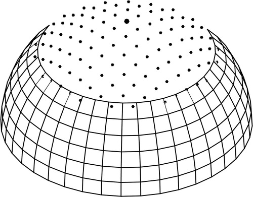
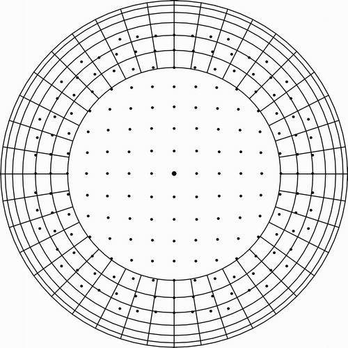
Fig. 2. Orthogonally projected grid system on the equatorial plane, with overlapping corresponding to the centred 4th order method, and with N= 40.

We will now briefly comment on some other methods considered in the literature. Our main sources are the two overview papers Staniforth and Thuburn (2012) and Williamson (2007). Let us first note that according to Staniforth and Thuburn (2012), most operational global NWP models are based on full latitude-longitude grids and semi-Lagrangian schemes (Robert, 1982; Lauritzen et al., 2010). By replacing a full latitude–longitude grid with our E-P grid system, the so called pole problem disappears and the number of gridpoints would be reduced by a factor of about two-thirds $(2/\pi )$.

There are many other grids and grid systems for the sphere, among the most popular are the cubed sphere and the icosahedral grids. Cubed sphere grids (Ronchi et al., 1996; Sadourny, 1972) consist of quadrilaterals and have been used for finite volume (Putman and Lin, 2007; Ullrich et al., 2010), discontinuous Galerkin (Bao et al., 2014; Nair et al., 2005), and finite difference methods (Ronchi et al., 1996). Some drawbacks of this grid system are lack of orthogonality, and deviation from uniformity. At eight points on the sphere, corresponding to the corner-points of the cube, there are angles up to 120° instead of the ideal 90°. Icosahedral grids (Williamson, 1968) are generally triangular and have been used for finite volume (Chen et al., 2014; Li and Xiao, 2010), and discontinuous Galerkin methods (Giraldo, 2006; Läuter et al., 2008). At 12 points there are angles up to 72° instead of the ideal 60°. We see no reason here to consider in detail the implications of these irregularities, consult (e.g. Peixoto and Barros, 2013). In Pudykiewics (2011), it is reported (in the Section 1) how important it can be to perform some kind of suitable grid regularisation, in order to improve the convergence rate of various quantities.

The great importance of the polar axis for the dynamics of the weather is indisputable, therefore we should require that grid systems have good symmetric properties relative this axis, as in Fig. 2. In Staniforth and Thuburn (2012), Section 3.5.2 is a grid system the authors call modified Yin–Yang, that at first glance bears resemblance to our E-P grid. It consists of an ordinary lat(θ)–lon(λ) grid, with $-45°\le \theta \le 45°$ and $0°\le \lambda \le 360$, and two polar grids, which can be obtained by moving the spherical quadrilateral ql of the equatorial grid corresponding to $-45°\le \theta \le 45°$ and $0°\le \lambda \le 90$ to the north and to the south by $90°$, respectively. The ql is not equilateral, the ratio between the longest and shortest edges is $\sqrt{2}$, which is also reflected in the shapes of the mesh rectangles. We refer to Figure 8(b) in Staniforth and Thuburn (2012), where the lack of symmetry relative the polar axis is obvious. For a three grid system these polar grids should not be used, since there are much better alternatives, cf. Section 2.3 and Fig. 1.

We also want to mention the interesting, overset Yin-Yang grid system (Kageyama and Sato, 2004; Qaddouri and Lee, 2011), developed in 2004. In a future paper, we plan to compare this with our E-P grid system. For the latter we will also experiment with letting the equatorial grid be a suitably reduced grid (cf. Gates and Riegel, 1963; Kurihara, 1965), in order to make it broader and to increase the uniformity. We admit that our E-P grid system does not quite share the classical and philosophical elegance of the Yin–Yang grid, but considering the above it might be more functional.

The article is organized as follows. In Section 2, we first express the shallow water equations in spherical and later in modified stereographic coordinates. Further, some centred difference approximations for first order derivatives are given.

In Section 3, the E-P grid system is defined and details concerning the underlying minimax problem are given. Further, overlapping and interpolation between grids with minimal overlapping are considered, depending on what we call strict overlapping, cf. Section 3.4.

Section 4 is devoted to numerical experiments. To evaluate our grid system we only consider the well-known high order centred difference methods, because of their low complexity. We present two groups of experiments, namely advection problems and problems for the non-linear shallow water equations. In the first group, we consider smooth deformational flow, and solid body rotations of the Cosine bell. The second group contains test problems 2, 3, and 6 from Williamson et al. (1992). For problems 2 and 3 we investigate whether any harmful grid imprinting occurs, and the answer is no. For problem 6, we study conservation properties for mass and energy.

The development of new methods generally involves many people and research publications. Thus, we will not state that our E-P grid systems is superior to, for example, the cubed sphere grid for NWP. However, the following list of advantages might be of interest: (i) Orthogonality and better uniformity, (ii) 3 grids instead of 6, (iii) the ideal latitude–longitude grid is used for a major part of the sphere, (iv) no harmful grid imprinting, cf. the test problems 2 and 3 in Section 4, (v) in Table 5, the Rossby–Haurwitz wave, the total mass is correct to about seven decimal digits, which is obviously much more than needed for NWP, (vi) possibility to let the equatorial grid be a reduced grid to increase the uniformity and by connecting to the polar grids sufficiently close to the poles, scalability problems can be avoided, and (vii) the computational results for the E-P grid system compare favourably with other alternatives, cf. Section 4.

Table 5. The Rossby–Haurwitz wave: Relative changes of the total mass and energy.

$re{l}_{\mathit{\text{mass}}}(1:7)$	1.27e − 7	2.43e − 7	2.59e − 7	2.94e − 7	1.55e − 7	−1.01e − 7	−3.31e − 7
$re{l}_{\mathit{\text{mass}}}(8:14)$	−3.59e − 7	−2.92e − 7	−1.35e − 7	2.13e − 8	9.88e − 8	1.32e − 8	−1.81e − 7
$re{l}_{\mathit{\text{energy}}}(1:7)$	4.24e − 4	1.70e − 3	3.32e − 3	4.47e − 3	5.01e − 3	5.46e − 3	5.70e − 3
$re{l}_{\mathit{\text{energy}}}(8:14)$	5.67e − 3	5.70e − 3	5.56e − 3	5.16e − 3	5.12e − 3	5.34e − 3	5.15e − 3

N = 360, 2p = 4, s = 2, c = 1.7e − 5, $\Delta t=120$s, Time =14 days.

Efficient parallel implementation of global methods for NWP are of course very important and are mostly performed by experts in HPC. The standard decomposition of the three grids in our E-P system is straight forward. The scalability considerations for the E-P and the Yin–Yang grid systems are very similar. In Kageyama and Sato (2004), the latter is used for mantle and geodynamo simulations on a parallel computer of distributive memory type, with 5120 vector-type processors. The conclusion of the authors in Kageyama and Sato (2004) is: ‘The Yin–Yang grid is suitable for massively parallel computers’. In this article, only the simplest version of an E-P grid system is considered in detail. However, the generalisation mentioned in (vi) above is probably more interesting and can completely avoid scalability problems in relation to the overlapping. Some additional aspects of implementation are given at the beginning of Section 4.

2 Coordinate systems, governing equations and some basic discrete formulas

Throughout this article, we assume that the solutions, with the velocity components appropriately expressed, are smooth on the entire sphere, in local Cartesian coordinates.

2.1. Spherical coordinates

The transformation between Cartesian and spherical coordinates is (1) $$\{\begin{array}{c}x=a\hspace{0.17em}\text{cos}\hspace{0.17em}\theta \hspace{0.17em}\text{cos}\hspace{0.17em}\lambda ,\hfill \\ y=a\hspace{0.17em}\text{cos}\hspace{0.17em}\theta \hspace{0.17em}\text{sin}\hspace{0.17em}\lambda ,0\le \lambda <2\pi ,-\frac{\pi }{2}\le \theta \le \frac{\pi }{2},\hfill \\ z=a\hspace{0.17em}\text{sin}\hspace{0.17em}\theta ,\hfill \end{array}$$(1) where a is the radius of the sphere, λ the longitude, and θ the latitude. The advective form of the shallow water equations in spherical coordinates is given by (2) $$\begin{array}{l}{u}_t=-{(a\hspace{0.17em}\text{cos}\hspace{0.17em}\theta )}^{-1}(u{u}_{\lambda }+{\Psi }_{\lambda })-a^{-1}v{u}_{\theta }+(f+a^{-1}u\hspace{0.17em}\text{tan}\hspace{0.17em}\theta )v,\\ v_t=-{(a\hspace{0.17em}\text{cos}\hspace{0.17em}\theta )}^{-1}u{v}_{\lambda }-a^{-1}(v{v}_{\theta }+{\Psi }_{\theta })-(f+a^{-1}u\hspace{0.17em}\text{tan}\hspace{0.17em}\theta )u,\\ {\Psi }_t=-{(a\hspace{0.17em}\text{cos}\hspace{0.17em}\theta )}^{-1}(u_{\lambda }\Psi +u{\Psi }_{\lambda })-a^{-1}{(v\Psi )}_{\theta }+a^{-1}v\Psi \hspace{0.17em}\text{tan}\hspace{0.17em}\theta ,\end{array}$$(2) where $\Psi$ is the geopotential, $f=2\Omega \hspace{0.17em}\text{sin}\hspace{0.17em}\theta$ the Coriolis parameter, Ω the rotation rate of the sphere, and finally, u and v the eastward and the northward velocity components, respectively. The system (2) will only be used in a band around the equator.

2.2. Stereographic coordinates

In our numerical experiments the polar regions $-\pi /2\le \theta \le -\pi /4$ and $\pi /4\le \theta \le \pi /2$, will be covered with grids corresponding to somewhat modified stereographic coordinates, considered in detail in Section 2.3 below. Let us first look at the standard stereographic coordinates, for which many formulas can be found in, for example Lanser et al. (2000). We express the relation between the two systems of coordinates as (3) $$\{\begin{array}{c}{x}_{st}=a q(\theta )\hspace{0.17em}\text{cos}\hspace{0.17em}\lambda ,\hfill \\ y_{st}=a q(\theta )\hspace{0.17em}\text{sin}\hspace{0.17em}\lambda ,\hfill \end{array}$$(3) where $q(\theta )=2\hspace{0.17em}\text{tan}(\phi /2)$, with the colatitude $\phi$ equal to $\frac{1}{2}\pi -\theta$ and $\frac{1}{2}\pi +\theta$, on the northern and southern hemisphere, respectively. We also need the map factor $m_f(\theta )=2/(1+\alpha \hspace{0.17em}\text{sin}\hspace{0.17em}\theta )$, where α = 1 on the northern and –n on the southern hemisphere.

Since the velocities in spherical coordinates, $u=a \hspace{0.17em}\text{cos}\hspace{0.17em}\theta d\lambda /dt$, $v=a d\theta /dt$, are not uniquely defined at the poles, we use instead the stereographic velocities $U=-d{x}_{st}/dt,V=d{y}_{st}/dt$. Observe the insertion of the minus sign in the definition of U, intended to get nicer formulas, namely (4) $$\left(\begin{array}{c}u\\ v\end{array}\right)=A\left(\begin{array}{c}U\\ V\end{array}\right)\text{and}\left(\begin{array}{c}u\\ -v\end{array}\right)=A\left(\begin{array}{c}U\\ V\end{array}\right),\text{where}A=\left(\begin{array}{cc}\hspace{0.17em}\text{sin}\hspace{0.17em}\lambda & \hspace{0.17em}\text{cos}\hspace{0.17em}\lambda \\ \hspace{0.17em}\text{cos}\hspace{0.17em}\lambda & -\hspace{0.17em}\text{sin}\hspace{0.17em}\lambda \end{array}\right),$$(4) on the northern and southern polar regions, respectively. Note that in Equation (4)(4) $$\left(\begin{array}{c}u\\ v\end{array}\right)=A\left(\begin{array}{c}U\\ V\end{array}\right)\text{and}\left(\begin{array}{c}u\\ -v\end{array}\right)=A\left(\begin{array}{c}U\\ V\end{array}\right),\text{where}A=\left(\begin{array}{cc}\hspace{0.17em}\text{sin}\hspace{0.17em}\lambda & \hspace{0.17em}\text{cos}\hspace{0.17em}\lambda \\ \hspace{0.17em}\text{cos}\hspace{0.17em}\lambda & -\hspace{0.17em}\text{sin}\hspace{0.17em}\lambda \end{array}\right),$$(4) , U and V have been scaled by the factor $1/m_f(\theta )$, for details see Lanser et al. (2000). The mapping (4) is also used in Starius (2014), but derived in a different way.

2.3. Modified stereographic coordinates

For stereographic coordinates the distances between consecutive gridpoints are decreasing, when we move towards the equator along a meridian, and the reduction factor from a pole to a parallel with latitude θ is $1/m_f(\theta )$. From the pole to the equator the distances between pairs of neighbouring gridpoints decrease by 50%. Stereographic projection is only suitable for grid generation when used quite locally. We therefore recommend a modification of (3) so that the spherical (1) and our new modified stereographic gridpoints will coincide for $\lambda =0,\frac{1}{2}\pi ,\pi$, and $\frac{3}{2}\pi$. This leads to more uniformity for the polar grids and will also simplify the connection between the equatorial and the modified stereographic grids. Since these will have common gridpoints on the meridians referred to above, it will be easy to define overlapping quantitatively. Further, the number of gridpoints in the polar regions will decrease and the amount of interpolation between grids can be somewhat reduced.

Let us introduce new coordinates $(x\prime ,y\prime )$, instead of $(x_{st},y_{st})$, by (5) $$x_{st}=\rho (x\prime )\text{and}{y}_{st}=\rho (y\prime ),\rho \left(0\right)=0,$$(5) where the function ρ is to be defined. For λ = 0, the case we consider here, we have y_st = 0 and from (3) by squaring and adding we get $$x_{st}=2a \hspace{0.17em}\text{tan}(\phi /2),\text{for}{y}_{st}=0.$$

By choosing $x\prime =\phi$ in the formula above and making a similar choice for y_st, we arrive at (6) $$\{\begin{array}{c}{x}_{st}=2a \hspace{0.17em}\text{tan}(x\prime /2),\hfill \\ y_{st}=2a \hspace{0.17em}\text{tan}(y\prime /2).\hfill \end{array}$$(6)

We now turn to the shallow water equations expressed in the coordinates defined in (3) and (6) and the stereographic velocities U and V, given in (4). From the shallow water equations in stereographic coordinates, cf. Lanser et al. (2000) or Browning et al. (1989), we easily obtain the equations in our modified coordinates (7) $$\begin{array}{c}{\left(\begin{array}{c}U\\ V\end{array}\right)}_t=\frac{m_f}{a}\left[ {\hspace{0.17em}\text{cos}\hspace{0.17em}}^2\frac{x\prime }{2} U{\left(\begin{array}{c}U\\ V\end{array}\right)}_{x\prime }-{\hspace{0.17em}\text{cos}\hspace{0.17em}}^2\frac{y\prime }{2} V{\left(\begin{array}{c}U\\ V\end{array}\right)}_{y\prime }+\left(\begin{array}{c}{\hspace{0.17em}\text{cos}\hspace{0.17em}}^2\frac{x\prime }{2} {\Psi }_{x\prime }\\ {\hspace{0.17em}\text{cos}\hspace{0.17em}}^2\frac{y\prime }{2} {\Psi }_{y\prime }\end{array}\right) \right]+[ \alpha f-\frac{1}{a}( \hspace{0.17em}\text{tan}\hspace{0.17em}\frac{x\prime }{2} V+\hspace{0.17em}\text{tan}\hspace{0.17em}\frac{y\prime }{2} U ) ]\left(\begin{array}{c}-V\\ U\end{array}\right),{\Psi }_t=\frac{m_f}{a}[ \hspace{0.17em}{\text{cos}}^2\frac{x\prime }{2} {(U\Psi )}_{x\prime }-\hspace{0.17em}{\text{cos}}^2\frac{y\prime }{2} {(V\Psi )}_{y\prime } ]-\frac{1}{a}[ \hspace{0.17em}\text{tan}\hspace{0.17em}\frac{x\prime }{2} U-\hspace{0.17em}\text{tan}\hspace{0.17em}\frac{y\prime }{2} V ]\Psi ,\end{array}$$(7) where the map factor m_f can be expressed as $$m_f=1+{\hspace{0.17em}\text{tan}\hspace{0.17em}}^2\frac{x\prime }{2}+{\hspace{0.17em}\text{tan}\hspace{0.17em}}^2\frac{y\prime }{2}.$$

As earlier α = 1 on the northern hemisphere and −1 on the southern.

2.4. Spatial discretisations

In our numerical experiments, given in Section 4, the following discretisations will be used. Replace first order derivatives by centred equidistant difference approximations of the wanted order 2p, say, in (2) and (7).

With $x_j=jh$, for some meshlength h, and $f_j=f(x_j)$, we write down a couple of approximations, for first order derivatives, with error terms (8) $$\begin{array}{c}hf\prime \left(x_j\right)=\frac{2}{3}(f_{j+1}-f_{j-1})-\frac{1}{12}(f_{j+2}-f_{j-2})+\frac{1}{30}{h}^5{f}^{\left(5\right)}\left({\xi }_2\right),\hfill \\ hf\prime \left(x_j\right)=\frac{3}{4}(f_{j+1}-f_{j-1})-\frac{3}{20}(f_{j+2}-f_{j-2})+\frac{1}{60}(f_{j+3}-f_{j-3})-\frac{1}{140}{h}^7{f}^{\left(7\right)}\left({\xi }_3\right),\hfill \\ hf\prime \left(x_j\right)=\frac{4}{5}(f_{j+1}-f_{j-1})-\frac{1}{5}(f_{j+2}-f_{j-2})+\frac{4}{105}(f_{j+3}-f_{j-3})-\frac{1}{280}(f_{j+4}-f_{j-4})+\frac{1}{630}{h}^9{f}^{\left(9\right)}\left({\xi }_4\right),\hfill \end{array}$$(8) where $x_{j-p}<{\xi }_p<x_{j+p}$, for p = 2, 3, 4.

3. Description of the grids and their connections by interpolation

We assume that the same physical meshlength is suitable everywhere, and that thus the grids should be as uniform as possible.

In the following the three grids in the E-P system will be referred to as: (i) The equatorial grid, (ii) the northern polar grid, and (iii) the southern polar grid. We will often consider only the northern hemisphere, because of symmetry with respect to the equator. Further, quadrilaterals on the sphere with right angles will be called rectangles or squares.

The E-P system will be uniquely determined by specifying the number of gridpoints, N say, on circles of parallel in the equatorial grid. We define $\Delta \lambda =2\pi /N$ and assume, because of symmetry, that 4 is a divisor of N. Further, denote the latitudinal meshlength by $\Delta \theta$, and let θ₀ be the latitude on the northern hemispheres, where the grids meet. In the present section $\Delta \theta$ and θ₀ will be determined by minimising the maximal deviation factor, defined in detail in Section 3.1, for the E-P system.

3.1. The equatorial grid with optimal uniformity

On a parallel with latitude θ, the distance between two consecutive gridpoints is $\Delta \lambda \hspace{0.17em}\text{cos}\hspace{0.17em}\theta$, provided the radius of the earth is used as the unit of length. In the λ and θ directions, the distances from a gridpoint to its closest neighbours should have a ratio as close to 1 as possible. For this reason we define the deviation factor for latitude θ as (9) $$d(\theta )=\max \left(\frac{\Delta \lambda \hspace{0.17em}\text{cos}\hspace{0.17em}\theta }{\Delta \theta },\frac{\Delta \theta }{\Delta \lambda \hspace{0.17em}\text{cos}\hspace{0.17em}\theta }\right)=\max (\sigma \hspace{0.17em}\text{cos}\hspace{0.17em}\theta ,{(\sigma \hspace{0.17em}\text{cos}\hspace{0.17em}\theta )}^{-1}),\text{where}\sigma =\Delta \lambda /\Delta \theta .$$(9)

We require σ to be greater than 1, since this will lead to a smaller maximal deviation factor, see Fig. 1. An immediate consequence is that $d(0)=\sigma$.

Let us now in detail consider the equatorial grid covering the region $|\theta |\le {\theta }_0$, where the value of θ₀ will be chosen later. Because of monotonicity we have (10) $$d_{max}=\underset{0\le \theta \le {\theta }_0}{\max }d(\theta )=\max (\sigma ,{(\sigma \hspace{0.17em}\text{cos}\hspace{0.17em}{\theta }_0)}^{-1}),$$(10) and again because of monotonicity, the minimum of the right hand side is obtained for σ satisfying the equation $\sigma ={(\sigma \hspace{0.17em}\text{cos}\hspace{0.17em}{\theta }_0)}^{-1}$, with solution $\sigma =1/\sqrt{\hspace{0.17em}\text{cos}\hspace{0.17em}{\theta }_0}$. Thus we have (11) $$d_{\mathit{\text{minmax}}}=\underset{\sigma }{\min }\max (\sigma ,{(\sigma \hspace{0.17em}\text{cos}\hspace{0.17em}{\theta }_0)}^{-1})=1/\sqrt{\hspace{0.17em}\text{cos}\hspace{0.17em}{\theta }_0},\text{for}\sigma =1/\sqrt{\hspace{0.17em}\text{cos}\hspace{0.17em}{\theta }_0}.$$(11)

3.2. The Equator–Pole grid system with minimal maximal deviation factor

Let us first define ϱ as the quotient $\ge 1$ of the areas of two net rectangles and ${\varrho }_{max}$ as its maximal value in a grid. Further let us again consider stereographic projection, which is a conformal mapping. The latter can be expressed for instance by saying that the mapping is locally a similarity transformation, or that the Jacobian of the transformation is an orthogonal matrix, multiplied by a scalar. This implies that the deviation factors are close to 1, but the value of ${\varrho }_{max}$ can be considerable, e.g. ${\varrho }_{max}=4$ for a hemisphere. Conformal mappings are often too inflexible for grid generation (cf. Starius, 1977b). In our modified stereographic coordinates the orthogonality is preserved and the uniformity properties are improved, in the sense that the values of ϱ become smaller. We do not actually use ϱ in the design of the E-P grid system.

For an orthogonal net only the deviation factors and the quotients ϱ are needed to measure uniformity. In our equatorial net the meshlength $\Delta \theta$ is kept constant, which implies that ${\varrho }_{max}=d_{\mathit{\text{minmax}}}^2$. Thus it suffices to minimise the maximal deviation factor in our equatorial net.

For the modified stereographic coordinates in Section 2.3, we choose $\Delta x\prime =\Delta y\prime =\Delta \theta .$ On the meridians $\lambda =0,\frac{1}{2}\pi ,\pi$, and $\frac{3}{2}\pi$, this will give equidistant gridpoints with distance $\Delta \theta$. The distance in the orthogonal direction will then be about $\Delta \theta /m_f(\theta )$, because for $y\prime$ of order $\Delta y\prime$, the stereographic y_st will differ only slightly from $y\prime$, cf. (6). At meridians $\pi /4+k\pi /2,k=0,1,2,3$ the net rectangles in the modified grid are almost squares and the deviation factors on a circle of parallel are maximal for $k\pi /2,k=0,1,2,3$. Thus, the maximal deviation factor in the northern polar grid is (12) $$\frac{\Delta \theta }{\Delta \theta /m_f\left({\theta }_0\right)}=m_f\left({\theta }_0\right)=\frac{2}{1+\hspace{0.17em}\text{sin}\hspace{0.17em}{\theta }_0}.$$(12)

The optimal value of θ₀ can therefore be determined by the equation, cf. Equations (11)(11) $$d_{\mathit{\text{minmax}}}=\underset{\sigma }{\min }\max (\sigma ,{(\sigma \hspace{0.17em}\text{cos}\hspace{0.17em}{\theta }_0)}^{-1})=1/\sqrt{\hspace{0.17em}\text{cos}\hspace{0.17em}{\theta }_0},\text{for}\sigma =1/\sqrt{\hspace{0.17em}\text{cos}\hspace{0.17em}{\theta }_0}.$$(11) and (12)(12) $$\frac{\Delta \theta }{\Delta \theta /m_f\left({\theta }_0\right)}=m_f\left({\theta }_0\right)=\frac{2}{1+\hspace{0.17em}\text{sin}\hspace{0.17em}{\theta }_0}.$$(12) , $$\frac{1}{\sqrt{\hspace{0.17em}\text{cos}\hspace{0.17em}{\theta }_0}}=\frac{2}{1+\hspace{0.17em}\text{sin}\hspace{0.17em}{\theta }_0},$$ with solution $180 {\theta }_0/\pi \approx 44.0603°$ corresponding to $d_{\mathit{\text{minmax}}}\approx 1.1797$. In all experiments in Section 4, we have used ${\theta }_0=\pi /4$, with $d_{\mathit{\text{minmax}}}\approx 1.1892$. Now when θ₀ and $\sigma =1/\sqrt{\hspace{0.17em}\text{cos}\hspace{0.17em}{\theta }_0}$ are known, we can evaluate $\Delta \theta =\Delta \lambda /\sigma$. Of practical reasons this value is modified by defining m₀ to be ${\theta }_0\sigma /\Delta \lambda$, rounded to the nearest integer and then defining a new $\Delta \theta ={\theta }_0/m_0$.

Let us briefly mention the frequently used ratio of maximum to minimum gridlength as a measure of uniformity. For our E-P grid system this ratio is minimised by using the equation $1/\hspace{0.17em}\text{cos}\hspace{0.17em}{\theta }_0=2/(1+\hspace{0.17em}\text{sin}\hspace{0.17em}{\theta }_0)$ with solution $\text{cos}({\theta }_0)=0.8$, $180 {\theta }_0/\pi \approx 36.87°$. The ratio is 1.25, which is small compared to other grids, cf. Section 3.3 in Staniforth and Thuburn (2012). For orthogonal meshes we prefer our own deviation factor (9), partly because it leads to smaller polar grids.

3.3. Extensions of the grids leading to overlapping

We require that the overlapping will make it possible to connect the different grids by centred interpolation formulas. The equatorial grid will be extended towards the poles by gridpoints on one or a few parallels, depending on the order of the scheme, and the polar grids will be extended towards the equator. We recall that on the meridian λ = 0, the step is $\Delta \theta$ in both grids, and further that they have one gridpoint in common, with latitude θ₀. We extend the equatorial grid so that it will cover the region $|\theta |\le {\theta }_1$, with $${\theta }_1={\theta }_0+s_1\Delta \theta =(m_0+s_1)\Delta \theta ,$$ where the non-negative integer s₁, chosen later, will be referred to as the overlapping number for the equatorial grid. In Section 3.4, we will extend the northern polar grid by using the latitude $${\theta }_2={\theta }_0-s_2\Delta \theta =(m_0-s_2)\Delta \theta ,$$ where the non-negative integer s₂, chosen later, is the overlapping number for the polar grids. The number $s=s_1+s_2$ is called the overlapping number for the grid system. How s can be chosen is given at the end of Section 3.4. With s given, we choose s₁ = s₂, for s even, and $s_1=(s+1)/2$ and $s_2=(s-1)/2$, for s odd.

In Fig. 2, the E-P system, for N= 40 and with the overlapping included, is orthogonaly projected on the equatorial plane. We notice, for example, that for N= 1000 the overlapping zone would hardly be visible.

3.4. Centred interpolation between grids and minimal overlapping

When we discretise on the grids by using one of the formulas in (8), values for the dependent variables are needed at some points outside the grid, but belonging to the stencil used. These points will be called interpolation points because the corresponding values will be determined by interpolation. In this article, we use centred bi-variate Lagrangian interpolation of order $2p+1$, where p is given by the order 2p for our centred discretisation. Points for which discretisations of the differential equations are used, will be called discretisation points.

The interpolation points for the equatorial grid are gridpoints on the parallels with latitude ${\theta }_1+k\Delta \theta ,k=1,\dots ,p$. The southern hemisphere is treated analogously. On the northern polar grid we proceed as follows. We approximate the circle of parallel corresponding to $\theta ={\theta }_2-\Delta \theta$ by a closed polygon having its corners at gridpoints of the northern polar grid, and with interior $\text{angles}\ge 3\pi /4$. This can be done in a step wise manner, in which each step consists of choosing among three appropriate grid points the one closest to the parallel. The points chosen will be interpolation points whose interior gridpoints are defined to be the discretisation points. By using the latter together with the stencil for our discretisation, the rest of the interpolation points on the northern polar grid can be determined. This procedure gives us good control over where the interpolation points of the northern polar grid will be placed in the equatorial grid, which is important when we want to minimise the overlapping. Because of symmetry with respect to the equator, no preparations concerning connections and interpolation formulas are needed for the southern polar grid.

We say that the overlapping is strict if the interpolation formulas only use discretisation points in other grids. A strict overlapping is called minimal if its overlapping number s is minimal.

Section 4.3.1 includes an example of an unstable scheme, using the E-P grid system, which violates the requirements of strict overlapping. We therefore recommend the use of strict overlapping for the kind of connections used in this article. This concept was introduced already in Starius (1980), but differently formulated and without a name.

Using our computer program we found that for our fourth and sixth order methods, minimal overlapping requires s= 2 and s= 3, respectively. Greater overlapping numbers s are of course possible. However, more than minimal overlapping can be meaningless, as we will see in Section 4.2.2.

4. Numerical experiments

In this section, we try to numerically evaluate the E-P grid system by considering a number of test examples, most of which are taken from Williamson et al. (1992). The spatial discretisations are given in Section 2.4, and for the time integration the classical explicit fourth order Runge–Kutta method is used, for which interpolations between grids are needed for each of the four stages. It is assume that the errors caused by each time integration below, not only ours, are small enough to be negligible in our comparisons between different methods for the SWE.

Methods for NWP must be able to use many thousands of processors in an efficient way, which favours the use of explicit time integration, since parallelisation can be considerably better and more easily implemented than for semi-implicit methods. Further, it might be desirable to resolve gravitational waves, which would make both ordinary explicit and exponential time integration methods (Clancy and Pudykiewics, 2013; Gaudreault and Pudykiewicz, 2016) more interesting.

Some further comments about the implementation. The variables U, V, and $\Psi$ on the southern and northern polar grids are represented by square matrices, corresponding to squares enclosing the polar circular regions. Gridpoints in the squares but not in the polar circular regions can be ‘enion in the computations, if this is considered to simplify the programming. By representing factors in Equation (7)(7) $$\begin{array}{c}{\left(\begin{array}{c}U\\ V\end{array}\right)}_t=\frac{m_f}{a}\left[ {\hspace{0.17em}\text{cos}\hspace{0.17em}}^2\frac{x\prime }{2} U{\left(\begin{array}{c}U\\ V\end{array}\right)}_{x\prime }-{\hspace{0.17em}\text{cos}\hspace{0.17em}}^2\frac{y\prime }{2} V{\left(\begin{array}{c}U\\ V\end{array}\right)}_{y\prime }+\left(\begin{array}{c}{\hspace{0.17em}\text{cos}\hspace{0.17em}}^2\frac{x\prime }{2} {\Psi }_{x\prime }\\ {\hspace{0.17em}\text{cos}\hspace{0.17em}}^2\frac{y\prime }{2} {\Psi }_{y\prime }\end{array}\right) \right]+[ \alpha f-\frac{1}{a}( \hspace{0.17em}\text{tan}\hspace{0.17em}\frac{x\prime }{2} V+\hspace{0.17em}\text{tan}\hspace{0.17em}\frac{y\prime }{2} U ) ]\left(\begin{array}{c}-V\\ U\end{array}\right),{\Psi }_t=\frac{m_f}{a}[ \hspace{0.17em}{\text{cos}}^2\frac{x\prime }{2} {(U\Psi )}_{x\prime }-\hspace{0.17em}{\text{cos}}^2\frac{y\prime }{2} {(V\Psi )}_{y\prime } ]-\frac{1}{a}[ \hspace{0.17em}\text{tan}\hspace{0.17em}\frac{x\prime }{2} U-\hspace{0.17em}\text{tan}\hspace{0.17em}\frac{y\prime }{2} V ]\Psi ,\end{array}$$(7) such as $$\frac{m_f}{a}{\hspace{0.17em}\text{cos}\hspace{0.17em}}^2\frac{x\prime }{2}\text{and}\frac{m_f}{a}{\hspace{0.17em}\text{cos}\hspace{0.17em}}^2\frac{y\prime }{2},\text{where}{m}_f=1+{\hspace{0.17em}\text{tan}\hspace{0.17em}}^2\frac{x\prime }{2}+{\hspace{0.17em}\text{tan}\hspace{0.17em}}^2\frac{y\prime }{2},$$ by the appropriate square matrices, element-wise multiplication can be applied with advantage. This means that the extra cost resulting from our modified stereographic coordinates will reduce to some negligible preprocessing.

In all the tables below, 2p is the order of approximation of the discretisations for (2) and (7). The order of the interpolation formulas connecting the grids is $2p+1$. The overlapping number for the grid system is denoted by s, as in Section 3.3. Modified stereographic coordinates are always used, except in Table 3.

Table 3. Normalized errors for steady state geostrophic flow.

α	${10}^8·c$	2p	s	stc, ${\ell }_{\infty }(\Psi )$	stc,  ${\ell }_2(\Psi )$	${10}^8·c$	mstc,  ${\ell }_{\infty }(\Psi )$	mstc,  ${\ell }_2(\Psi )$
0	2.5	4	2	7.4896e − 8	2.7333e − 8	2.0	2.3393e − 8	1.4434e − 8
45	94.5	4	2	4.5811e − 6	7.1803e − 7	15.0	9.8324e − 7	1.3341e − 7
90	3.5	4	2	3.3136e − 7	1.4239e − 7	3.5	3.3416e − 7	1.5007e − 7
0	0	6	3	3.2131e − 10	1.0983e − 10	0	1.7475e − 11	8.0196e − 12
45	0	6	3	4.9529e − 8	2.4985e − 9	0	3.7105e − 10	1.0249e − 10
90	0	6	3	5.7385e − 10	2.2245e − 10	0	4.1246e − 10	2.0270e − 10

N = 240, $\Delta t=300$s, Time =5 days, stc: = stereographic coord. and mstc: = modified stereographic coord.

The geopotential $\Psi =gH$, where g is the acceleration of gravity and H the height of the fluid. The relative error norms ${\ell }_2(H)$ and ${\ell }_{\infty }(H)$, introduced in Williamson et al. (1992), will be used.

4.1. Smoothing

Smoothing is essential for the centred finite difference methods to work properly and will be achieved by adding a so called hyper-diffusion term to each equation in (2) and (7). Since hyper-diffusion has no known physical meaning, we consider our smoothing a purely numerical process, used for carefully stabilizing the scheme. We do not aim at making our centred scheme less oscillatory by smoothing. Actually, the oscillatory behaviour decreases in the order of the centred scheme, cf. Table 2.

Table 2. Normalized errors for solid rotation of the Cosine bell.

α	${10}^8·c$	2p	s	$\min H$	$\max H$	${\ell }_{\infty }(H)$	${\ell }_2(H)$
90	98.5	4	2	−7.4455	9.9906e + 2	7.4455e − 3	6.5382e − 3
87	101.5	4	2	−7.4175	9.9904e + 2	7.4175e − 3	6.5323e − 3
45	43.0	4	2	−6.2911	9.9758e + 2	6.2919e − 3	7.2938e − 3
90	98.5	4	3	−7.4441	9.9907e + 2	7.4452e − 3	6.5374e − 3
87	102.0	4	3	−7.4151	9.9904e + 2	7.4169e − 3	6.5313e − 3
90	14.5	6	3	−2.7415	9.9958e + 2	2.7466e − 3	2.3972e − 3
87	12.0	6	3	−2.7398	9.9956e + 2	2.7844e − 3	2.5172e − 3
87	12.0	8	4	−1.6730	1.0000e + 3	1.6995e − 3	2.2057e − 3

N = 360, $\Delta t=600$s, Time =12 days, $\min {\ell }_{\infty }(H)$.

Let L_h be the five-point operator for the Cartesian form of the Laplacian, that is $$L_h{u}_{i,j}=-4u_{i,j}+u_{i+1,j}+u_{i,j+1}+u_{i-1,j}+u_{i,j-1}.$$

To the first, the second, and the third system in Equation (2)(2) $$\begin{array}{l}{u}_t=-{(a\hspace{0.17em}\text{cos}\hspace{0.17em}\theta )}^{-1}(u{u}_{\lambda }+{\Psi }_{\lambda })-a^{-1}v{u}_{\theta }+(f+a^{-1}u\hspace{0.17em}\text{tan}\hspace{0.17em}\theta )v,\\ v_t=-{(a\hspace{0.17em}\text{cos}\hspace{0.17em}\theta )}^{-1}u{v}_{\lambda }-a^{-1}(v{v}_{\theta }+{\Psi }_{\theta })-(f+a^{-1}u\hspace{0.17em}\text{tan}\hspace{0.17em}\theta )u,\\ {\Psi }_t=-{(a\hspace{0.17em}\text{cos}\hspace{0.17em}\theta )}^{-1}(u_{\lambda }\Psi +u{\Psi }_{\lambda })-a^{-1}{(v\Psi )}_{\theta }+a^{-1}v\Psi \hspace{0.17em}\text{tan}\hspace{0.17em}\theta ,\end{array}$$(2) , we add the terms $-c{L}_h^{2}u,-c{L}_h^{2}v$, and $-c{L}_h^2\Psi$, respectively. In (7), U and V are used instead of u and v. We observe that $L_h^2\Psi =O(\Delta {\theta }^4)$, for any smooth function $\Psi$. Note that in the discretisations the smoothing terms will be multiplied by $\Delta t$. The smoothing constant $c\ge 0$ is approximately determined by numerically minimising ${\ell }_2(H)$. In Section 4.2.2 ${\ell }_{\infty }(H)$ is minimised instead. We have used the MATLAB^® routine fminbnd.

We have also tried to let L_h correspond to a five-point difference approximation to the Laplacian in spherical coordinates. Not surprisingly, this did not improve the results, which seems natural since our grids are almost uniform.

4.2. Advection test problems

We recall that the advective equation $dH/dt=0$ is linear, generally with variable coefficients, and describes conservation of mass.

4.2.1. Smooth deformational flow, stationary vortex

In this first example two vortices will be created during the time integration and their positions can be given by a parameter, which makes it possible to place their centres in our overlapping zones. The details can be found in Nair and Jablonowski (2008). We give a short summary here, partly because we are going to use some of the formulas in this section also in Section 4.3.2.

Let $(\lambda \prime ,\theta \prime )$ be a rotated spherical coordinate system whose North pole, $(\lambda \prime ,\pi /2)$, is located at $({\lambda }_p,{\theta }_p)$ in another spherical system $(\lambda ,\theta )$. By Nair and Jablonowski (2008), the transformation between the two spherical coordinate systems can be written (13) $$\begin{array}{c}\hspace{0.17em}\text{tan}\hspace{0.17em}\lambda \prime (\lambda ,\theta )=\frac{\hspace{0.17em}\text{cos}\hspace{0.17em}\theta \hspace{0.17em}\text{sin}(\lambda -{\lambda }_p)}{\hspace{0.17em}\text{cos}\hspace{0.17em}\theta \hspace{0.17em}\text{sin}\hspace{0.17em}{\theta }_p\hspace{0.17em}\text{cos}(\lambda -{\lambda }_p)-\hspace{0.17em}\text{cos}\hspace{0.17em}{\theta }_p\hspace{0.17em}\text{sin}\hspace{0.17em}\theta }\\ \hspace{0.17em}\text{sin}\hspace{0.17em}\theta \prime (\lambda ,\theta )=\hspace{0.17em}\text{sin}\hspace{0.17em}\theta \hspace{0.17em}\text{sin}\hspace{0.17em}{\theta }_p+\hspace{0.17em}\text{cos}\hspace{0.17em}\theta \hspace{0.17em}\text{cos}\hspace{0.17em}{\theta }_p\hspace{0.17em}\text{cos}(\lambda -{\lambda }_p).\end{array}$$(13)

The vortices will be created with centres at the poles of the system $(\lambda \prime ,\theta \prime )$ and will later be transformed to the system $(\lambda ,\theta )$. The normalized tangential velocity of the vortex is defined to be $V=v_0\frac{3\sqrt{3}}{2}\frac{\tanh (\rho )}{{\cosh }^2(\rho )}$, where $\rho ={\rho }_0\hspace{0.17em}\text{cos}(\theta \prime )$ is the radial distance of the vortex, and ${\rho }_0=3$. In the initial condition (cf. Nair and Jablonowski, 2008), γ = 5, and the velocity $v_0=2\pi a/T$, where T is the total time of the simulation, set to be 12 days. For this deforming vortex case the angular velocity ω varies and is defined to be $\omega (\theta \prime )=V(\rho )/(a\rho )$, and we let ω = 0, for $\theta \prime =\pm \pi /2$.

In Nair and Jablonowski (2008), the zonal and meriodinal velocities are given, in the system $(\lambda ,\theta )$, by (14) $$\begin{array}{c}u=a\omega (\theta \prime )[\text{sin}\hspace{0.17em}{\theta }_p\hspace{0.17em}\text{cos}\hspace{0.17em}\theta -\hspace{0.17em}\text{cos}\hspace{0.17em}{\theta }_p\hspace{0.17em}\text{cos}(\lambda -{\lambda }_p)\hspace{0.17em}\text{sin}\hspace{0.17em}\theta ],\\ v=a\omega (\theta \prime )\hspace{0.17em}\text{cos}\hspace{0.17em}{\theta }_p\hspace{0.17em}\text{sin}(\lambda -{\lambda }_p).\end{array}$$(14)

Further set ${\lambda }_p=\pi$ and $\alpha =\pi /2-{\theta }_p$, where the parameter α is the opening angle between the North poles of the two spherical systems, seen from their common origin. We mention that in the system $(\lambda ,\theta )$ the case α = 0 means that the centres of the vortices are at the poles and the flow is along circles of parallel, and $\alpha =90°$ means that the centres are on the equator. Since our grids are connected at latitudes $\theta =\pm \pi /4$, the value $\alpha ={45}^o$ is of particular interest to us, because the centres of the vortices will be located on parallels corresponding to these latitudes, cf. Fig. 3.

Fig. 3. Contour curves for smooth deformational flow: $\alpha ={45}^o$, N = 240, 2p = 4 and Time=12 days.

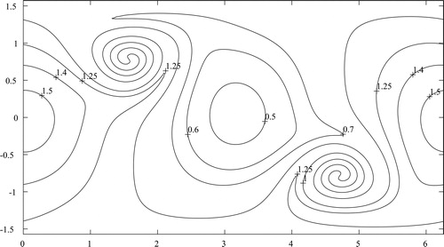
In Table 1 the ${\ell }_2(\Psi )$ errors, the ones we have minimised, are actually smallest for $\alpha =45°$, which indicates that the connections between grids work quite well.

Table 1. Normalized errors for smooth deformational flow, stationary vortex.

α	${10}^8·c$	2p	s	$\min \Psi$	$\max \Psi$	${\ell }_{\infty }(\Psi )$	${\ell }_2(\Psi )$
0	1.0	4	2	0.46295	1.5370	4.9954e − 3	6.4872e − 4
45	3.5	4	2	0.46299	1.5370	4.9587e − 3	5.6236e − 4
90	1.6	4	2	0.46297	1.5370	7.5553e − 3	1.0074e − 3
0	0.25	6	3	0.46295	1.5370	1.1315e − 3	1.2714e − 4
45	0.35	6	3	0.46299	1.5370	1.1612e − 3	1.0952e − 4
90	0.45	6	3	0.46297	1.5370	2.1246e − 3	2.4623e − 4

N = 240, $\Delta t=400$s, Time =12 days.

We conclude by some convergence results for $\alpha =45°$ and use (2p, N, $\Delta t,{10}^{8}c,{\ell }_2(\Psi )$) for the corresponding computation. From (4, 240, 300, 1.1, 2.1457e − 5), (4, 360, 200, 0.7, 4.3405e − 6) we get the order 3.94(4) and (6, 240, 150, 0.080, 1.4892e − 6), (6, 360, 100, 0.030, 1.4129e − 7) give the computed order 5.81(6). The above computed orders of approximation are a bit too small, which probably depends on lack of smoothness or resolution at the centers of the vortices.

4.2.2 Rotation of the cosine bell

In this example, we consider a solid body rotation of the Cosine bell, according to test problem no. 1 in Williamson et al. (1992). The advecting wind is given by $$u=u_0(\text{cos}\hspace{0.17em}\theta \hspace{0.17em}\text{cos}\hspace{0.17em}\alpha +\hspace{0.17em}\text{sin}\hspace{0.17em}\theta \hspace{0.17em}\text{cos}\hspace{0.17em}\lambda \hspace{0.17em}\text{sin}\hspace{0.17em}\alpha ),v=-u_0\hspace{0.17em}\text{sin}\hspace{0.17em}\lambda \hspace{0.17em}\text{sin}\hspace{0.17em}\alpha ,$$ where α is the angle between the axis of the solid body rotation and the polar axis, and $u_0=2\pi a/12$ m/day. Only cases when the bell passes the parallels $\theta =\pm \pi /4$ will be considered in Table 2. In this example, we have minimised ${\ell }_{\infty }(H)$ instead of ${\ell }_2(H)$, in order to be able to make some comparisons at the end of this section.

In rows 4 and 5 of Table 2, we have used more overlapping, s = 3, than was needed, which led to no real increase in accuracy. This is one of the reasons we recommend minimal overlapping.

In Ronchi et al. (1996), an interesting gridding technique is introduced by combining the cubed sphere decomposition with overlapping grids. For the present problem their spatial discretisation is a centred fourth order difference scheme, used with N = 360 and $\Delta t=600$s. The main difference compared to our method, is in the choice of the grid system. For $\alpha ={45}^o$ corner points of the cube are inside the support of the bell during about one-third of a revolution. Unfortunately, for this case cancellations of errors occur, which distorts our comparison between the methods. We mention that the $1000·{\ell }_{\infty }(H)$ error in Ronchi et al. (1996) is 7.33 and ours is 6.29.

For $\alpha =90°$ the $1000·{\ell }_{\infty }(H)$ error in Ronchi et al. (1996) is 10.17 and ours is 7.45. For given resolution, the error in Ronchi et al. (1996) can only be marginally decreased, by our or other grid systems, since the track of their Cosine bell is along a meridian passing through the midpoints on four edges, cf. figures in Staniforth and Thuburn (2012) and Williamson (2007), and thus displays the best uniformity possible, for the Cubed sphere grid. The mesh covering this track is almost uniform.

We conclude this example by some convergence results. Despite the solutions are only in $C^1(\mathit{\text{sphere}})$ the errors, ${\ell }_{\infty }(H)$ in Table 2, are decreasing fairly rapidly in the formal orders of approximation. As usual, lower bounds for the errors are settled by the continuous problem and the used grid and its resolution. We have minimised $c\to {\ell }_2(H)$, with N = 240, $\Delta t=900$s and later with N = 360, $\Delta t=600$s and got the computed orders 2.17, 2.19 and 2.33, corresponding to the formal orders 4, 6 and 8, respectively.

4.3. Non-linear shallow water test problems

In the present section, we study the time integration of the complete inviscid shallow water equations.

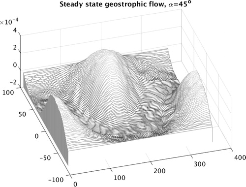
4.3.1. Steady state geostrophic flow

We now consider test problem no. 2 from Williamson et al. (1992), which constitutes a steady state solution to the shallow water equations. The advecting wind is the same as for the Cosine bell. The parameter α is the angle between the North poles of the systems $(\lambda ,\theta )$ and $(\lambda \prime ,\theta \prime )$, both having the centre of the earth as their origin. For the latter system the pole $(\lambda \prime ,\pi /2)$ coincides with the North pole of the earth. The solution corresponds to solid body rotation and zonal flow in the system $(\lambda \prime ,\theta \prime )$. To express the Coriolis parameter f and the geopotential $\Psi$ in the coordinates $(\lambda ,\theta )$, the relation $\text{sin}\hspace{0.17em}\theta \prime =\hspace{0.17em}\text{sin}\hspace{0.17em}\theta \hspace{0.17em}\text{cos}\hspace{0.17em}\alpha -\hspace{0.17em}\text{cos}\hspace{0.17em}\theta \hspace{0.17em}\text{cos}\hspace{0.17em}\lambda \hspace{0.17em}\text{sin}\hspace{0.17em}\alpha$ is useful. We have $f=2\Omega \hspace{0.17em}\text{sin}\hspace{0.17em}\theta \prime$ and $\Psi ={\Psi }_0-(a\Omega u_0+u_0^2/2){\hspace{0.17em}\text{sin}\hspace{0.17em}}^2\theta \prime$, where ${\Psi }_0=2.94·{10}^4$ and $u_0=2\pi a/12$ m/day.

Numerical results are presented in Table 3, both for stereographic and modified stereographic coordinates. For $\alpha ={45}^o$ there are significant differences. This case is more sensitive than the other two, with $\alpha =0^o\text{and}{90}^o$, for which the wind fields are along parallels and mainly along meridians, respectively. For $\alpha =45°$ the directions of the wind often form an angle of about $45°$ with parallels. The superiority of the modified stereographic grid, in particularly for the order 6, must be caused by the better uniformity. From now on we restrict ourselves to these coordinates, for which the errors in Table 3 are fairly the same for $\alpha =45°$ and $\alpha =90°$. For $\alpha =0°$ the solutions are much simpler than for the other cases, which explains the higher accuracy.

In an additional experiment, not presented in a table, we replaced s= 2 with s= 1 in the third row of Table 3, which implied that a lot of points used in interpolation formulas were interpolation points from another grid, so that the requirement of strict overlapping was violated. The scheme was unstable ($\min \Psi <8·{10}^3$ before 10 days), up to about c= 70 and then stabilized. The minimal ${\ell }_2$ error, occurring for $c\sim 1000$, was about 900 times larger than for the case s= 2 in Table 3. This shows that strict overlapping should be used for the kind of connections considered here.

In Ullrich et al. (2010), a fourth order finite volume method on a cubed sphere grid, having 25 points in its stencil, is used for $\alpha =45°$, and with N = 160 and N= 320 gridpoints on the equator. We compare it with our 6th order method, having only 13 points in its stencil. The ${\ell }_2$ errors in Ullrich et al. (2010) are about 90 and 520 times larger than ours for N= 160 and N= 320, respectively. We could have used the 4th order difference method instead, with only 9 points in its stencil, but the corresponding comparisons would be too unbalanced, since the amount of computational work per gridpoint is also important, not only the order of approximation. Unfortunately, the above is not a clear-cut comparison between grid systems.

We now consider some convergence results, for $\alpha =45°$, and use the same notation as in our first example. From (4, 240, 300, 15.0, 1.3341e − 7), (4, 360, 200, 12.5, 2.5275e − 08) we get the computed order 4.10(4). Similarly from (6, 240, 200, 0, 1.0253e − 10), (6, 360, 200, 0, 9.0908e − 12) we arrive at the computed order 5.98(6).

In Fig. 4, we have visualised the error ${\Psi }_{\mathit{\text{computed}}}-\Psi$ as function of latitude and longitude. The true solution $\Psi$ has two minimum points per period, namely $\theta =45°,\lambda =180°$ and $\theta =-45°,\lambda =0°$ or $360°$. In the vicinities of these points the curvature is much greater than elsewhere, which leads to much larger errors in these vicinities. Everything in the figure can easily be explained by the solution $\Psi$, thus there is no harmful grid imprinting.

Fig. 4. Absolute errors as function of lat–lon, with 2p = 6, N = 240 and $\Delta t=300$.

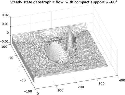
4.3.2 Steady state geostrophic flow with compact support

We now continue with test problem no. 3 from Williamson et al. (1992). The spherical coordinate systems $(\lambda \prime ,\theta \prime )$ and $(\lambda ,\theta )$ are the same as in Section 4.2.1 and the problem is formulated in the former system. For the velocity components $(u\prime ,v\prime )$, in the system $(\lambda \prime ,\theta \prime )$ we have $v\prime =0$ and $u\prime$ depends only on $\theta \prime$ and has compact support (cf. Williamson et al., 1992). The geopotential $\Psi$ is determined by an ordinary differential equation. Transformation to the rotated system $(\lambda ,\theta )$ leads to the same expression for the Coriolis parameter as in Section 4.3.1 and initial conditions were obtained by using Equations (13)(13) $$\begin{array}{c}\hspace{0.17em}\text{tan}\hspace{0.17em}\lambda \prime (\lambda ,\theta )=\frac{\hspace{0.17em}\text{cos}\hspace{0.17em}\theta \hspace{0.17em}\text{sin}(\lambda -{\lambda }_p)}{\hspace{0.17em}\text{cos}\hspace{0.17em}\theta \hspace{0.17em}\text{sin}\hspace{0.17em}{\theta }_p\hspace{0.17em}\text{cos}(\lambda -{\lambda }_p)-\hspace{0.17em}\text{cos}\hspace{0.17em}{\theta }_p\hspace{0.17em}\text{sin}\hspace{0.17em}\theta }\\ \hspace{0.17em}\text{sin}\hspace{0.17em}\theta \prime (\lambda ,\theta )=\hspace{0.17em}\text{sin}\hspace{0.17em}\theta \hspace{0.17em}\text{sin}\hspace{0.17em}{\theta }_p+\hspace{0.17em}\text{cos}\hspace{0.17em}\theta \hspace{0.17em}\text{cos}\hspace{0.17em}{\theta }_p\hspace{0.17em}\text{cos}(\lambda -{\lambda }_p).\end{array}$$(13) and (14)(14) $$\begin{array}{c}u=a\omega (\theta \prime )[\text{sin}\hspace{0.17em}{\theta }_p\hspace{0.17em}\text{cos}\hspace{0.17em}\theta -\hspace{0.17em}\text{cos}\hspace{0.17em}{\theta }_p\hspace{0.17em}\text{cos}(\lambda -{\lambda }_p)\hspace{0.17em}\text{sin}\hspace{0.17em}\theta ],\\ v=a\omega (\theta \prime )\hspace{0.17em}\text{cos}\hspace{0.17em}{\theta }_p\hspace{0.17em}\text{sin}(\lambda -{\lambda }_p).\end{array}$$(14) . In the last set of formulas $a\omega (\theta \prime )$ should be replaced by $u\prime /\hspace{0.17em}\text{cos}\hspace{0.17em}\theta \prime$. The results are presented in Fig. 5 and Table 4.

Fig. 5. Geostrophic flow with compact support, with $\alpha =60°$ and N= 240.

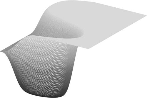
Table 4. Normalized errors for geostrophic flow with compact support.

α	${10}^8·c$	2p	s	$\min \Psi$	$\max \Psi$	${\ell }_{\infty }(\Psi )$	${\ell }_2(\Psi )$
0	7.0	4	2	2.0572e + 4	2.9401e + 4	4.4288e − 6	1.1233e − 6
60	10.5	4	2	2.0572e + 4	2.9401e + 4	2.0841e − 5	4.0558e − 6
0	0	6	3	2.0572e + 4	2.9401e + 4	7.5006e − 8	1.3479e − 8
60	0	6	3	2.0572e + 4	2.9401e + 4	2.8129e − 7	5.3725e − 8

N = 240, $\Delta t=300$s, Time =5 days.

In Browning et al. (1989), two overlapping stereographic grids are used together with a centred difference method of order 6. The resolution compares well to our N= 240. Only the case α = 0 was considered and the ${\ell }_2$ error was $6.6·{10}^{-5}$, which is about $4.9\times {10}^3$ times larger than our error. The grid system in Browning et al. (1989) is different from ours, with much less uniformity. Nevertheless, the difference in accuracy seems surprisingly high.

The order of approximation will now be estimated experimentally, according to Williamson et al. (1992), for $\alpha =60°$ and for our method of formal order 4. The resolutions are determined by N = 160, $N=1.5\times 160=240$, and $N=1.5\times 240=360$, all with $\Delta t=150$s. With smoothing parameter ${10}^{8}c=10$, in all three cases, we find the ${\ell }_2$ errors $2.4309\times {10}^{-5},4.0756\times {10}^{-6}$, and $7.8697\times {10}^{-7}$. By using the first two and the last two errors, we found the approximate orders 4.404 and 4.056, respectively. By optimising each case, we found the ${10}^{8}c$ values 21, 11.5, and 8.5, and the ${\ell }_2$ errors $2.1458\times {10}^{-5},4.0715\times {10}^{-6}$, and $7.8630\times {10}^{-7}$, and the corresponding orders 4.099 and 4.056.

The general features of Fig. 6 can be explained by using Fig. 5 and comments similar to those made for Fig. 4. We conclude that there is no harmful grid imprinting in this case either.

Fig. 6. Absolute errors as function of lat–lon, with 2p = 6, N = 240 and $\Delta t=300$.

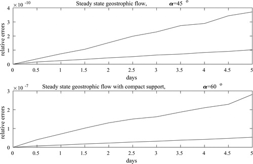
In Fig. 7, we give time traces of normalised errors, for the two geostrophic flow problems in Williamson et al. (1992). The ${\ell }_2(\Psi )$ errors, the ones that were minimised over c at the endpoint five days, grow linearly in time with no visible deviation.

Fig. 7. Test problems no. 2 and 3 from Williamson et al. (1992). In each panel the lower curve correspond to ${\ell }_2(\Psi )$ and the upper to ${\ell }_{\infty }(\Psi )$. In all cases 2p = 6, N = 240 and $\Delta t=300$.

4.3.3 Conservation properties of mass and energy for the Rossby–Haurwitz wave

We will use test problem no. 6 from Williamson et al. (1992) in order to study the global conservation properties for mass and energy. This test example was already used in Phillips (1959) and with a numerical procedure in some aspects related to our E-P based method. The integral formulas for mass and energy can be found in, for example Starius (2014). All dependent variables were interpolated to a full latitude–longitude grid before the numerical integration. The sum of squares of the relative errors for the total mass after each day, $\left|\right|re{l}_{\mathit{\text{mass}}}(1:14)|{|}_2$, was minimised over c.

In Table 5, we have used exactly the same numerical method as described earlier, without any corrections or fixers of any kind. The schemes does not explicitly conserve mass, but nevertheless the accuracy in the total mass over time is considerable, probably because of cancellation of errors. This situation is not new to us (cf. Starius, 1977a, 1977b). About seven significant decimal digits in the total mass is obviously sufficient for NWP. The relative changes in the total energy seem to be satisfactory, but are much larger than for the total mass. This is probably because, for non-linear problems, energy can move between different wave numbers.

5. Summary

We have introduced a new grid system for the sphere, called E-P, consisting of one equatorial and two polar grids. The former is an ordinary spherical latitude–longitude grid and the latter ones correspond to suitably modified stereographic coordinates. All grids are orthogonal and almost uniform and are connected by minimal overlapping and centred interpolation formulas, for dependent variables.

The superiority of the modified stereographic coordinates compared to the standard ones is most apparent in Table 3, for the two cases with $\alpha =45°$.

The uniformity is optimised in Section 3 by using so called deviation factors, cf. (9) and (12), for the whole grid system. The comparisons made between different grid systems, in Sections 4.2.2, 4.3.1 and 4.3.2, clearly indicate the usefulness of uniformity, which would probably be more pronounced for more typical wave propagation problems. In a forthcoming paper, we plan to return to this point in connection with a comparison between the well-known overset Yin–Yang and our E-P grid systems. Also, a generalisation of the E-P system will be considered by letting the equatorial grid be a suitable reduced grid (cf. Gates and Riegel, 1963; Kurihara, 1965). This will improve the uniformity and increase the area covered by the equatorial grid considerably, and decrease the total number of gridpoints, and be important for wave propagation problems. Further, the circular polar grids, used in this article, will be compared to the use of square polar grids. They are, at the least, somewhat easier to implement, but there might be other differences as well.

In this short article, all focus is on our overset E-P grid system, which can be looked upon as a way to concentrate the unavoidable non-uniformity to narrow bands, where it is handled by overlapping and accurate centred interpolation formulas.

Disclosure statement

No potential conflict of interest was reported by the author.

References

- Bao, L., Nair, R. D. and Tufo, H. M. 2014. A mass and momentum flux-form higher-order discontinuous Galerkin shallow water model on the cubed-sphere. J. Comput. Phys. 271, 224–243. doi:10.1016/j.jcp.2013.11.033.
- Browning, B. L., Hack, J. J. and Swarztrauber, P. N. 1989. A comparison of three numerical methods for solving differential equations on the sphere. Mon. Wea. Rev. 117, 1058–1075. doi:10.1175/1520-0493(1989)117<1058:ACOTNM>2.0.CO;2.
- Chen, C., Li, X., Shen, X. and Xiao, F. 2014. Global shallow water models based on multi-moment constrained finite volume method and three quasi-uniform spherical grids. J. Comput. Phys. 271, 191–223. doi:10.1016/j.jcp.2013.10.026.
- Clancy, C. and Pudykiewics, J. A. 2013. On the use of exponential time integration methods in atmospheric models. Tellus A 65, 20898. doi:10.3402/tellusa.v65i0.20898.
- Gates, W. L. and Riegel, A. 1963. A study of numerical errors in the integration of barotropic flow on a spherical grid. JGR 67, 406–423.
- Gaudreault, S. and Pudykiewicz, J. A. 2016. An efficient exponential time integration method for the numerical solution if the shallow water equations on the sphere. J. Comput. Phys. 322, 827–848. doi:10.1016/j.jcp.2016.07.012.
- Giraldo, F. X. 2006. High-order triangle-based discontinuous Galerkin methods for hyperbolic equations on a rotating sphere. J. Comput. Phys. 214, 447–465. doi:10.1016/j.jcp.2005.09.029.
- Henshaw, W. D. and Schwendeman, D. W. 2006. Moving overlapping grids with adaptive mesh refinement for high-speed reactive and non-reactive flow. J. Comput. Phys. 216, 744–779. doi:10.1016/j.jcp.2006.01.005.
- Ii, S. and Xiao, F. 2010. A global shallow water model using high order constrained finite volume method and icosahedral grid. J. Comput. Phys. 229, 1774–1796. doi:10.1016/j.jcp.2009.11.008.
- Kageyama, A. and Sato, T. 2004. The Yin-Yang grid: An overset grid in spherical geometry. Geochem. Geophys. Geosyst. 5, Q09005.
- Kurihara, Y. 1965. Integration of the primitive equations on a spherical grid. Mon. Wea. Rev. 93, 399–415. doi:10.1175/1520-0493(1965)093<0399:NIOTPE>2.3.CO;2.
- Lanser, D., Blom, J. G. and Verwer, J. G. 2000. Spatial discretisation of the shallow water equations in spherical geometry using Osher’s scheme. J. Comput. Phys. 165, 542–565. doi:10.1006/jcph.2000.6632.
- Lauritzen, P. H., Nair, R. D. and Ullrich, P. A. 2010. A conservative semi-Lagrangian multi-tracer scheme (CSLAM) on a cubed-sphere grid. J. Comput. Phys. 229, 1401–1424. doi:10.1016/j.jcp.2009.10.036.
- Läuter, M., Giraldo, F. X., Handorf, D. and Dethloff, K. 2008. A discontinuous Galerkin method for the shallow water equations using spherical triangular coordinates. J. Comput. Phys. 227, 10226–10243. doi:10.1016/j.jcp.2008.08.019.
- Nair, R. D. and Jablonowski, C. 2008. Moving vortices on the sphere: A test case for horizontal advection problems. Mon. Wea. Rev. 136, 699–711. doi:10.1175/2007MWR2105.1.
- Nair, R. D., Thomas, S. J. and Loft, R. D. 2005. A discontinuous Galerkin transport scheme on the cubed sphere. Mon. Wea. Rev. 133, 814–828. doi:10.1175/MWR2890.1.
- Peixoto, P. S. and Barros, S. R. M. 2013. Analysis of grid imprinting on geodesic spherical icosahedral grids. J. Comput. Phys. 237, 61–78. doi:10.1016/j.jcp.2012.11.041.
- Phillips, N. A. 1959. Numerical integration of the primitive equations on the hemisphere. Mon. Wea. Rev. 87, 333–345. doi:10.1175/1520-0493(1959)087<0333:NIOTPE>2.0.CO;2.
- Pudykiewics, J. A. 2011. On numerical solution of the shallow water equations with chemical reactions on icoshedral geodesic grid. J. Comput. Phys. 230, 1956–1991. doi:10.1016/j.jcp.2010.11.045.
- Putman, W. M. and Lin, S.-J. 2007. Finite-volume transport on various cubed-sphere grids. J. Comput. Phys. 227, 55–78. doi:10.1016/j.jcp.2007.07.022.
- Qaddouri, A. and Lee, V. 2011. The Canadian global environmental multiscale model on the Yin-Yang grid system. Qjr. Meteorol. Soc. 137, 1913–1926. doi:10.1002/qj.873.
- Robert, A. 1982. A semi-Lagrangian and semi-implicit numerical integration scheme for the primitive meteorological equations. J. Meteorol. Soc. Jpn. 60, 319–325. doi:10.2151/jmsj1965.60.1_319.
- Ronchi, C., Iacono, R. and Paolucci, P. S. 1996. The cubed sphere: A new method for the solution of partial differential equations in spherical geometry. J. Comput. Phys. 124, 93–114. doi:10.1006/jcph.1996.0047.
- Sadourny, R. 1972. Conservative finite-differencing of the primitive equations on quasi-uniform spherical grids. Mon. Wea. Rev. 100, 136–144. doi:10.1175/1520-0493(1972)100<0136:CFAOTP>2.3.CO;2.
- Staniforth, A. and Thuburn, J. 2012. Horizontal grids for global weather and climate prediction models: a review. Qjr. Meteorol. Soc. 138, 1–26. doi:10.1002/qj.958.
- Starius, G. 1977a. Composite mesh difference methods for elliptic boundary value problems. Numer. Math. 28, 243–258. doi:10.1007/BF01394455.
- Starius, G. 1977b. Constructing orthogonal curvilinear meshes by solving initial value problems. Numer. Math. 28, 25–48. doi:10.1007/BF01403855.
- Starius, G. 1980. On composite mesh difference methods for hyperbolic differential equations. Numer. Math. 35, 241–255. doi:10.1007/BF01396411.
- Starius, G. 2014. A solution to the pole problem for the shallow water equations on a sphere. TWMS JPAM. 5, 152–170.
- Ullrich, P. A., Jablonowski, C. and van Leer, B. 2010. High-order finite-volume methods for the shallow-water equations on the sphere. J. Comput. Phys. 229, 6104–6134. doi:10.1016/j.jcp.2010.04.044.
- Volkov, E. A. 1968. The method of composite meshes for finite and infinite regions with piecewise smooth boundaries. Proc. Steklov Inst. Math. 96, 145–185.
- Williamson, D. L. 1968. Integration of the barotropic vorticity equation on a spherical geodesic grid. Tellus. 20, 642–653.
- Williamson, D. L. 2007. The evolution of dynamical cores for global atmospheric model. JMSJ. 85B, 241–269. doi:10.2151/jmsj.85B.241.
- Williamson, D. L., Drake, J. B., Hack, J. J., Jakob, R. and Swarztrauber, P. N. 1992. A standard test set for numerical approximation to the shallow water equations in spherical geometry. J. Comput. Phys. 102, 211–224. doi:10.1016/S0021-9991(05)80016-6.