Evolution of observed ozone, trace gases, and meteorological variables over Arrival Heights, Antarctica (77.8°S, 166.7°E) during the 2019 Antarctic stratospheric sudden warming

Abstract

We use ground-based spectroscopic remote sensing measurements of the stratospheric trace gases O₃, HCl, ClO, BrO, HNO₃, NO₂, OClO, ClONO₂, N₂O and HF, along with radiosonde profiles of temperature to track the springtime development of the 2019 ozone hole over Arrival Heights (77.8°S, 166.7°E, AHTS), Antarctica, during, and after, the 2019 stratospheric sudden warming (SSW) event. Both measurements and model simulations show that the 2019 SSW caused an extraordinarily warm stratosphere within the polar vortex, resulting in record low ozone depletion over AHTS. We also contrast the evolution of the 2019 ozone hole to that in 2002, which also had a major springtime SSW event.

The SSW event started around 28^th August. By ∼17^th September, stratospheric temperatures inside the polar vortex over AHTS were ∼45 K higher than the climatological average. The SSW did not cause an en masse displacement of mid-latitude air over AHTS as in the 2002 SSW event. However, the increased temperatures did cause an unusually early reduction in polar stratospheric clouds, halting the denitrification early and leading to increased gas-phase HNO₃ and record high levels of NO₂ (‘renoxification’). This caused the earliest observed deactivation of chlorine, returning all active chlorine into the chlorine reservoir species, HCl and ClONO₂. The deactivation rate into HCl remained relatively unaffected by the SSW, whilst there was a dramatic increase in ClONO₂ formation. This chlorine deactivation pathway via ClONO₂ is typical of the Arctic and atypical for the Antarctic.

At AHTS, record high levels of springtime ozone were observed. The measured ozone total column did not drop below 220 DU. Record high stratospheric temperatures persisted until 7^th October over AHTS. By 22^nd October, AHTS was not beneath the polar vortex. The polar vortex break-up date on 9^th November was one of the earliest observed.

Keywords:

• Arrival Heights
• Antarctica
• stratospheric sudden warming
• polar heterogeneous ozone depletion chemistry

1. Introduction

Major stratospheric sudden warmings in the northern hemisphere (NH) are defined by a wind reversal (westerlies to easterlies) at 60°N and 10 hPa (Charlton and Polvani, 2007; Baldwin et al., 2021). From mid-late August through to mid-September 2019 the mean zonal wind at 10 hPa inside the Antarctic polar vortex slowed from ∼90 ms⁻¹ to ∼10 ms⁻¹, causing anomalously rapid and large warming (∼40 K over 3 days) of the upper stratosphere (10 hPa) (Newman et al., 2020; Wargan et al., 2020).

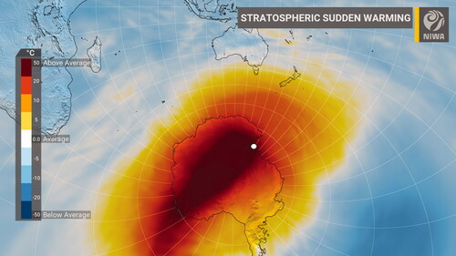
By the NH definition, Antarctic SSWs are rare. The last major SSW event occurring in 2002 (Shepherd et al., 2005), and prior to that, 1988 (Kanzawa and Kawaguchi, 1990). The 2019 Antarctic SSW was forecast and attributed to a persistent strong stationary (zonal wavenumber 1) upward propagating planetary wave (Lim et al., 2020; Rao et al., 2020; Shen et al., 2020; Yamazaki et al., 2020). The 2019 SSW caused record high stratospheric temperatures within the polar vortex, up to 50 K warmer (at 10 hPa) than the climatological mean (Fig. 1). Because it lacked a wind reversal, it is considered a minor SSW.”

Fig. 1. ERA5 reanalysis 10 hPa temperature at local midnight 12^th September 2019 compared to the 1981-2010 climatology. The 12^th September 2019 being the approximate date of peak temperature anomaly (Yamazaki et al., 2020). Arrival Heights (77.8°S, 166.7°E) is shown as a white dot. MERRA2 temperature anomaly is like that of ERA5.

Polar ozone depletion driven by heterogeneous chemistry is now a well-known and well-documented phenomenon (Solomon, 1999; Brasseur and Solomon, 2005; von Clarmann and Johansson, 2018). Heterogeneous chemical reactions occur on liquid or solid ice particles whose presence depends strongly on temperature. The reactions convert halogen reservoir species, such as HCl and ClONO₂, into Cl₂, which is converted to active chlorine forms (e.g. Cl, HOCl, ClO) under sunlight conditions. The radicals participate in catalytic ozone loss cycles responsible for ozone depletion. Observational studies such as Newman et al. (2006) and Strahan et al. (2014) illustrate the effect of temperature and halogen abundance on Antarctic ozone hole area.

The impacts of SSWs on stratospheric ozone depletion have previously been observed in the Antarctic during 1988, 2002 and 2010 (e.g. Kanzawa and Kawaguchi, 1990; Hoppel, et al. 2003; Frieß et al., 2005; Ricaud et al., 2005; de Laat and van Weele, 2011), and during numerous Arctic SSW events (e.g. von Clarmann and Johansson, 2018). Under such circumstances, the warming of the polar stratosphere during the critical winter and spring seasons reduces the overall ozone depletion by limiting polar stratospheric cloud (PSC) formation, which in turn reduces denitrification, and returns active chlorine to reservoir species, resulting in higher than usual HCl and ClONO2 abundances. Additionally, renitrification increases gas phase HNO₃ assisting chlorine deactivation through formation of ClONO₂ (Douglass et al., 1995; Santee et al., 1995; Solomon et al., 2015; von Clarmann and Johansson, 2018). Readers are directed towards Douglass et al. (1995) and Nakajima et al. (2020) for succinct summaries of polar middle atmosphere chemistry.

During 2002 there was a series of austral winter and spring wave events beginning in May and culminating in a SSW on 22^nd September (Newman and Nash, 2005). The timing of the 2002 waves were important; the largest in late-September (Stolarski et al., 2005) caused polar vortex displacement, dilution and eventual (and unprecedented) splitting of the vortex (Glatthor et al., 2005). The displacement and dilution caused warming of the stratosphere accelerating chlorine deactivation (Grooß et al., 2005) and entrainment of mid-latitude ozone-rich airmasses to higher latitudes (Frieß et al., 2005). Overall, the 2002 SSW caused one of the smallest and least persistent ozone holes recorded; thus, we expect the 2019 SSW to have a similar effect on the 2019 ozone hole.

In this study we use radiosonde temperature soundings and ground based remote sensing of ozone and trace gases over AHTS, Antarctica, Modern Era Reanalysis for Research and Applications 2 (MERRA2) meteorological reanalysis products, and the Global Modelling Initiative chemical transport model (GMI CTM) to observe and simulate the temporal evolution of the 2019 ozone hole and the influence of the 2019 SSW on ozone depletion. We contrast this to the development of the 2002 ozone hole. In both years, we will show that despite the dynamical differences, the chemical pathways that deactivated reactive chlorine were about the same because warming leads to renitrification and conversion of ClO to ClONO2, which is typical of the Arctic and atypical of the Antarctic.

The following section (2) details the measurements, model and meteorological fields used in this study. In section 3 we investigate the development of the 2019 stratospheric temperatures and polar vortex dynamics over AHTS. Stratospheric long-lived tracer species N₂O and HF are discussed in section 4. In section 5 we display and comment on the temporal evolution of eight stratospheric trace gases: HNO₃, NO₂, HCl, ClONO₂, ClO, OClO, BrO and O₃; each playing a part of polar heterogeneous ozone chemistry. Finally, we provide a summary in section 6.

2. Measurements, model and meteorological fields

Ground based measurements of stratospheric trace gases and radiosonde soundings are made at three sites on Hut Point Peninsula, Ross Island. Scott Base, McMurdo Station and AHTS are located within a ∼5 km radius of each other. Both McMurdo Station and Scott Base are at sea level whereas the altitude at AHTS is 184 metres. For convenience we will collectively refer to the location of these three sites as ‘Arrival Heights’ and use the longitude and latitude of AHTS as the proxy coordinates for all three sites (77.8°S, 166.7°E).

At a latitude of 77.8°S, polar night (last sunset to first sunrise) extends 24^th April to 21^st August (non-leap years). From 21^st August onwards, the presence of late winter sunlight and extremely low temperatures allow heterogeneous ozone depletion to occur over AHTS. The vortex typically confined within the area bounded by 60°-90°S. Thus AHTS is often quite deep in the vortex and in most years the polar vortex remains intact until late October (Kreher et al., 1996; Wood et al., 2004; Frieß et al., 2005). However, when the polar vortex dynamics (shape, displacement and rotation) is unusual, AHTS can also reside underneath, on the edge, or outside of the polar vortex changing on a near-daily basis.

2.1. Remote sensing of trace gases

Stratospheric trace gas composition measurements started on Ross Island in 1982 (McKenzie and Johnston, 1984) and with campaigns at McMurdo in the 1980s (De Zafra et al., 1987; Farmer et al., 1987; Solomon et al., 1987). Such measurements provided trace gas measurements critical to the development of polar heterogeneous ozone chemistry theories (Solomon, 1999). The long-term availability of ground-based measurements to monitor the chemical composition of the stratosphere was the driving force behind the establishment of the Network for the Detection of Stratospheric Change (NDSC), now called the Network for the Detection of Atmospheric Composition Change, (NDACC), (Kurylo, 1991; De Mazière et al., 2018). All three Antarctic sites were founding stations of NDSC, and measurements continue to this day with an expanded range of instrumentation. The multitude of measurements at AHTS provides a unique long term combined observational dataset for chemical model and satellite comparisons and validation. Table 1 details the current instrumentation and measurements used in this study.

Table 1. Details of instrumentation and measurements used in this study.

Instrument	Location	Measurement type	Dataset length	Species	Reference
ADAS2	Arrival Heights	UV/Vis zenith-sky Czerny Turner grating spectrometer (UV 345 − 384 nm VIS 402 − 440 nm)	2002-2019	BrO, NO2, O3, OClO	Frieß et al. (2005)
Bruker120m and 125HR	Arrival Heights	Direct-sun mid infrared Fourier transform interferometer (800–4200 cm^-1)	1996-2019	ClONO2, HCl, HF, HNO3, N2O	Kohlhepp et al. (2012) Ronsmans et al. (2016) Vigouroux et al. (2007)
ChlOE1	Scott Base	Microwave radiometer (278.63 GHz)	1996-2019	ClO	Nedoluha et al. (2016)
Dobson	Arrival Heights	UV spectrophotometer (300–350 nm)	1988-2019	O3	Nichol (2018)
Radiosonde	McMurdo	RS92 and RS41-SGP in-situ soundings, twice daily (0, 12 UTC)	2016-2019	Pressure, Temperature	Dirksen et al. (2020)

The Dobson spectrophotometer, ADAS2 UV/Vis spectrometer and mid-infrared Fourier transform interferometer (FTIR) require sunlight. The ADAS2 zenith-sky measurements start on 19^th August and even earlier if higher SZA’s (e.g. up to 93° SZA) are used. In contrast, direct sun FTIR and Dobson measurements can start on 30^th August and 9^th September respectively. In 2019 the solar-based measurements at AHTS started a week before the onset of the observed SSW (∼28^th August, see section 3).

The Chlorine Oxide Experiment (ChlOE1) ground-based millimetre wave spectrometer at Scott Base is not reliant on sunlight, but instead monitors the weak molecular rotational emission lines of ClO, thus allowing measurements throughout the polar night before sunrise (Nedoluha et al., 2016). ClO has a strong diurnal cycle. There is little ClO at night, and by subtracting the night-time spectra from the daytime spectra we can minimize systematic instrumental artefacts in this demanding measurement. For the microwave measurements we have defined day as the period from 3 h after sunrise to 1 h before sunset, and night as the period from 4 h after sunset to 1 h before sunrise.

All observations continued over the 2019-2020 austral spring and summer seasons. Combinations of such simultaneous remote sensing trace gas measurements allows us to track the chemical development of springtime ozone depletion (e.g. Mellqvist et al., 2002; Adams et al., 2013 and Nakajima et al., 2020). The FTIR, Dobson and ChlOE1 datasets are available at the NDACC public repository: http://ftp.cpc.ncep.noaa.gov/ndacc/station/.

2.2. Radiosonde soundings at McMurdo

Radiosonde soundings of pressure, temperature, relative humidity and winds have been conducted twice daily since 1956 as part of operational weather forecasting for the McMurdo airfields. Operational sonde data are archived by the Antarctic Meteorological Research Center, USA (Stearns and Young, 1994) and available at http://ftp://amrc.ssec.wisc.edu/pub/mcmurdo/radiosonde. Being an operational product, data harmonization for long term trend analysis is not a priority, thus differences (biases) are expected when sonde make/model, pre-launch checks and data processing are changed. The large stratospheric temperature changes due to the SSW are easily detected, but to achieve a better level of consistency we only analyse data from February 2016 onwards which are all received and processed using common software (Vaisala DigiCORA® Sounding System MW41 2.3.0). The sondes routinely reach a height of 50 hPa in springtime. Radiosonde balloon burst height is typically between 30 to 50 hPa due to the cold conditions. The benefit of a harmonized McMurdo radiosonde dataset was recognised by the Global Climate Observing System (GCOS) Reference Upper-Air Network (GRUAN). Along with ground-based measurements made at Scott Base and AHTS, a Ross Island distributed GRUAN site is currently under certification review (Dirksen et al., 2020).

2.3. The global modelling initiative chemical transport model and meteorological reanalysis fields

Simulations of polar ozone depletion from the Global Modelling Initiative chemical transport model (GMI) (Strahan et al., 2007) are used in this study. GMI has complete gas-phase and heterogeneous chemistry schemes (Duncan et al., 2007), allowing comparison with, and added interpretation of, the ground-based measurements. GMI model simulations have previously been used to diagnose the effect of SSWs on ozone in the Arctic (Strahan et al., 2016). GMI is driven by global meteorological fields from the Modern Era Retrospective-Analysis for Research and Applications reanalysis product (MERRA2) (Gelaro et al., 2017). The GMI-MERRA2 MR2V3 data sets used in this study are stored in the public NDACC repository (http://ftp.cpc.ncep.noaa.gov/ndacc/gmi_model_data/). The data consists of yearly NetCDF files of daily data, for each NDACC FTIR site (including AHTS) on a 72-level pressure grid (surface level pressure to 0.01 hPa). GMI chemical species used in this study are HNO₃, NO₂, HCl, ClONO₂ and O₃.

Since ClO is not included in the standard publicly available GMI NDACC site datasets. ClO simulations for 2002 and 2019 (at 0 and 12Z) were additionally extracted from the GMI simulations for this study. To provide comparable model output to the ClO microwave radiometer, daily ClO day-night differences (0Z - 12Z) were computed. The ClO microwave radiometer at Scott Base has a fixed viewing direction looking south, with a line-of-sight elevation of ∼5° (85° SZA). This gives the 20 km tangent height ∼200 km south of AHTS (∼79.6°S, compared to 77.8°S) with sunrise approximately 3 days later than at AHTS. GMI ClO was in better agreement with measurements when this higher latitude data were used.

Potential vorticity over AHTS and the Southern Hemisphere polar vortex edge are extracted from MERRA2 analysis and used to diagnose when AHTS is underneath the polar vortex and to estimate the approximate date of the polar vortex break up. National Center for Environmental Prediction (NCEP) daily temperature profile data are used as a priori information for the FTIR retrievals (Gelman et al., 1994). Comparison of NCEP and MERRA2 temperature fields show near identical agreement.

3. Polar vortex evolution and stratospheric temperatures above AHTS

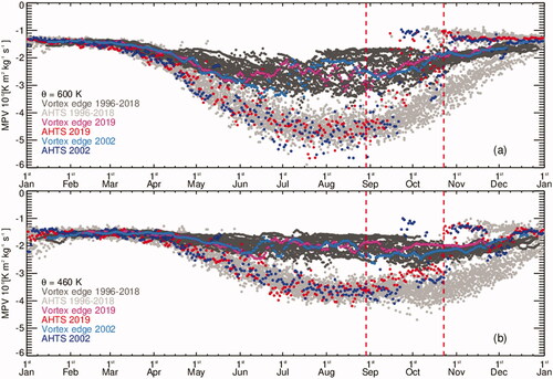
We use isentropic modified potential vorticity (MPV) (Lait, 1994) over AHTS and of the southern hemisphere polar vortex edge as a diagnostic of air mass origin. By comparing AHTS MPV to that of the vortex edge, we can infer if airmasses above AHTS are inside the vortex, outside the vortex or on the edge. An AHTS MPV value less than the vortex edge MPV indicates the airmass measured is inside the vortex. Although not being a definitive binary diagnostic, the difference in values does provide some indication of the proximity of AHTS to the vortex edge. Such a diagnostic has been used in prior studies using AHTS measurements (Kreher et al., 1996; Wood et al., 2004; Frieß et al., 2005; Schofield et al., 2006). Two isentropic MPV levels were chosen: 460 K and 600 K. For these theta levels, approximate altitudes over AHTS in late winter are 19 and 23 km respectively (and 17 and 21 km by late September). 460 K goes from ∼45 to 70 hPa (late August to late September) while 600 K goes from ∼20 to 38 hPa. The range includes altitudes of significant ozone depletion every year. Whilst the selected levels are relatively close together, the MPV on each surface exhibit slightly different dynamic behaviour relevant to interpreting the remotely sensed trace gas measurements and changes in lower-middle stratospheric temperature over AHTS.

The temporal development of lower-middle stratospheric temperature over AHTS at 30 hPa and 50 hPa is illustrated in Fig. 2. Both NCEP and sonde temperatures are well above climatological averages over the period 28^th August to 22^nd October. The reported onset of the 2019 SSW varies from 25^th August to 29^th August (Lim et al., 2020; Rao et al., 2020; Safieddine et al., 2020). Over AHTS on ∼8^th August NCEP 30 hPa and 50 hPa temperatures are below average, and below the Nitric Acid Trihydrate (NAT) PSC formation temperatures, ∼192 K and ∼195 K at each pressure respectively (Pitts et al., 2013) (Fig. 2). Temperatures start to increase thereafter and by 28^th August they are at or above the maximum temperatures since year 2000 but still cold enough to support PSCs. The 600 K and 460 K MPV levels indicate that the polar vortex is still over AHTS (Figs. 3a and b, respectively).

Fig. 2. 30 hPa and 50 hPa temperatures over AHTS from NCEP (panels A and B). McMurdo sonde 50 hPa temperature (panel C). Years with significant SSW events (2002 and 2019) are highlighted. The two vertical dashed red lines at 28^th August and 22^nd October indicate the onset on the 2019 SSW at AHTS and the last day AHTS is located beneath the polar vortex before vortex breakup. The black horizontal perforated line indicates the approximate formation temperature of NAT PSCs (∼192 K at 30 hPa and ∼195 K at 50 hPa). Supercooled ternary solution (STS) and water ice (ICE) PSCs form at temperatures lower than NAT formation temperatures.

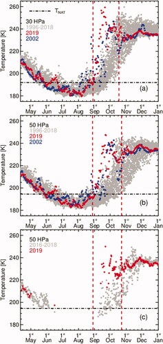
Fig. 3. MERRA2 MPV at AHTS and the SH polar vortex edge at (a) 600 K and (b) 460 K isentropic levels over the years 1996 to 2019. Years 2002 and 2019 are highlighted.

From 28^th August to 7^th September there is a rapid temperature increase at 30 hPa (from 192 K to 210 K) and at 50 hPa (from 193 K to 203 K) that exceeds PSC formation temperatures at both levels (Fig. 2). We define the onset of the 2019 SSW observed at AHTS as the 28^th August, coinciding with an unprecedented 35 K temperature increase at 10 hPa (not shown). From 28^th August to 7^th September, 600 K and 460 K MPV shows that AHTS remains under the vortex at both levels (Fig. 3).

From 7^th September to 27^th September there is an extraordinary increase in temperature of 30 K at both pressure levels (peaking at a 45 K increase at 50 hPa). 460 K MPV still remains less than the vortex edge MPV. Unlike 460 K, MPV at 600 K begins to exceed climatological values in early September and exceeds vortex edge values on many days between mid-September and mid-October, indicating that airmasses above AHTS oscillate between air inside, outside and on the edge of the vortex The observed high variability over AHTS occurs because the vortex has rotated and been displaced over the South American sector of Antarctica (Safieddine et al., 2020; Wargan et al., 2020). At ∼22^nd September AHTS 600 K MPV decreases (∼ −3 MPV units) along with a decrease in temperature (-15 K) indicating vortex rotation back over AHTS. This is a short interlude, with rotation quickly taking AHTS out from underneath the vortex in a matter of days. The large dynamical variability at 600 K is not seen on the 460 K isentropic level. The 460 K MPV shows that AHTS remains inside the vortex from 7^th September through to 12^th October.

From 12^th October to 22^nd October temperatures remain higher than average but are back within climatological norms with overall less variability. On the 22^nd October there is a rapid increase in temperatures at 50 hPa, and a steep increase in AHTS MPV at both 460 K and 600 K levels. From the 22^nd October onwards, AHTS is not underneath the polar vortex at either level. The vortex remains intact but displaced towards the South American side of Antarctica with eventual dissolution on 9^th November. The 2019 vortex break-up is one of the earliest vortex break ups on record (Bodeker and Kremser, 2020; Wargan et al., 2020).

The most significant dynamical differences between the 2002 and 2019 SSWs are in the waves causing the vortex disturbance (wave 1 displacement in 2019 versus a wave 2 split in 2002) and in the timing (Figs. 2 and 3). The 2002 ozone hole has been well characterised in general (e.g. Hoppel et al., 2003; Ricaud et al., 2005) and specifically, over AHTS (Frieß et al., 2005). In 2019 the 10 hPa zonal mean winds did not reverse, as in 2002, and the first significant warming events started around 25^th August 30 days earlier than 2002. While stratospheric temperature and heat flux anomalies were comparable between the years, the 2019 vortex remained intact and did not split as in 2002. On 24^th September 2002, at AHTS, temperatures increased along with MPV. Unlike 2019, 2002 AHTS 460 K MPV exceeded vortex edge MPV, this lasted until ∼7^th October, when the remaining fraction of the vortex was above AHTS until 22^nd October (coincidentally the same day as 2019). From 22^nd October until breakdown the vortex was not above AHTS. The 2002 vortex split caused a large movement of mid-latitude airmasses over AHTS at both 600 K and 460 K levels. In sections 4 and 5, we compare the evolution of long-lived gases over AHTS in 2002 and 2019.

4. Using HF and N₂O as tracers of polar vortex dynamics

Both long-lived species HF and N₂O have been used extensively as tracers of polar vortex stratospheric dynamics (e.g. Toon et al., 1999; Strahan et al., 2015 and Ricaud et al., 2005). At high latitudes, the two tracers can be used to measure diabatic descent (subsidence) and tropopause height changes within the polar vortex (Mellqvist et al., 2002). Both HF and O₃ increase with altitude in the lower stratosphere where most of their mass resides, hence vertical motions have similar effects on their column abundances. Subsidence causes HF inside the polar vortex to be of greater abundance than outside the vortex. Contrary to HF, N₂O abundance decreases with altitude. Hence subsidence causes stratospheric vortex air to have less N₂O than outside the vortex. N₂O isopleths have been used to define vortex edge in prior studies (e.g. Ricaud et al., 2005). Both HF and N₂O have been shown to have a high correlation with potential vorticity as shown in studies by Mellqvist et al. (2002), and Müller and Günther (2003) respectively. These two tracers can be used to aid us in diagnosing the origin of stratospheric airmasses over AHTS.

The evolution of HF and N₂O is consistent with the dynamics indicated by MPV and temperature in the previous section. Figure 4 displays HF (total) and N₂O (lower-middle stratospheric) columns measured at AHTS along with GMI N₂O partial columns (HF is not a simulated species). In 2019, both HF and N₂O measurements remain relatively constant throughout the SSW event and then up to 22nd October. There is no sudden decrease in HF or increase in N₂O measurements between 7th and 27th September, where temperatures increased by up to ∼30 K due to the SSW. Like the measurements, GMI N₂O partial column shows no rapid change in abundance from 7th to 27th September when rapid changes in temperature are observed. The lack of change in HF and N₂O indicates there is no major poleward movement of mid-latitude airmasses over AHTS, which would alter chemical composition and temperature of the stratosphere. Using N₂O tracer simulations, Wargan et al. (2020) also demonstrates that mixing below 600 K has a relatively small role in 2019. On 22nd October, measurements show a stepwise N₂O increase of ∼60% and HF decrease of ∼20%. There is also the expected abrupt steep in GMI N₂O on 22nd October. At the same time, the temperature and MPV increase rapidly on both levels shown, as noted in section 3. After 27th October, in all years, N₂O becomes more variable.

Fig. 4. (a) N₂O lower to mid stratosphere partial column (12–28 km) measured at AHTS. (b) GMI N₂O partial column (150 to 13 hPa, ∼12.5–28km) over AHTS. (c) HF total column measured at AHTS.

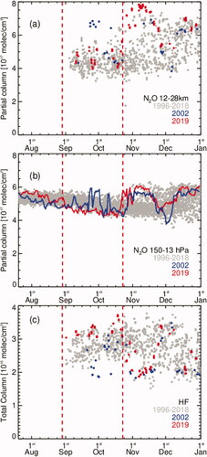
The 2002 HF and N₂O measurements, along with GMI simulations of N₂O (highlighted as blue in Fig. 4), provide an interesting contrast to that in 2019. In 2002 when the vortex split a mid-latitude airmass moved over AHTS from day ∼24^th September to 7^th October (Frieß, 2005). Over this period elevated levels of N₂O along with relatively low levels of HF were present, again correlating with AHTS MPV changes.

From the MPV diagnostics along with temperature and long-lived tracers, we conclude that in 2019 the polar vortex remained largely intact over AHTS until 22^nd October. At the 600 K level, the MPV diagnostics does show that vortex edge air was present over AHTS, and at the 460 K level the AHTS MPV is above climatological norms but still within the vortex. Nevertheless, the N₂O and HF tracers indicate that the effect of such air mass entrainment was minimal. The 2019 measured and modelled trace gas composition in the lower stratosphere over AHTS from late August through mid-October shows that it was predominantly affected by temperature changes and descent within the vortex rather than mixing processes across the vortex edge as occurred in 2002.

5. Temporal evolution of key ozone depleting species

This section presents the development during September and October of ozone and seven odd nitrogen or halogen-containing species involved in heterogeneous ozone depleting reactions. They are HNO₃, NO₂, HCl, ClONO₂, ClO, OClO, BrO, and ozone.

5.1. Nitric acid (HNO₃)

Stratospheric HNO₃ is a key component in the formation of PSCs and its reduced gas phase abundance during polar winter indicates PSC activity (Solomon et al., 2014). PSC formation requires very low stratospheric temperatures. NAT and STS PSC formation reduces the abundances of gas phase HNO₃ and H₂O, while the subsequent sedimentation of large PSCs (e.g. ice particles) causes denitrification and dehydration of the polar lower stratosphere. The warmer temperatures observed during a SSW event causes PSCs to evaporate, returning HNO₃ to the gas-phase (renitrification).

There are currently no ground-based PSC measurements on Ross Island. A 532 nm Rayleigh polarization lidar capable of PSC detection and classification operated at McMurdo station over the period 1991-2010 under the auspices of NDACC (Adriani et al., 2004). Analysis of the McMurdo lidar data over the period 2006-2010 by Snels et al. (2019) show that NAT PSCs account for the majority of PSC composition over the altitude range 15-25 km. Analysis of solar and lunar FTS HNO₃ measurements at AHTS by Wood et al. (2004) over the period 1998 to 2003 showed the expected correlations between stratospheric temperature, PSCs and gas phase HNO₃. Stratospheric water vapour is currently not measured at AHTS by remote-sensing or in situ soundings.

Measurements of HNO₃ and GMI HNO₃ simulations are shown in Fig. 5a and b respectively. In spring 2019 the first HNO₃ measurements were made on 30^th August. This single day of measurements shows the expected low levels of HNO₃. The 30 hPa and 50 hPa temperatures on this day are above the climatological average but below NAT formation temperatures (see Fig. 2). Together, the low abundances of HNO₃ and temperature data indicate the likely presence of PSCs. The measurements taken on 7^th September show a large increase in HNO₃ from ∼1.0 × 10¹⁸ to 1.8 × 10¹⁸ molec/cm², consistent with the sudden rise in observed temperature that exceeded the NAT formation temperature. This shows there was a temporary sequestration of gas-phase HNO₃ to NAT PSCs, not permanent denitrification via sedimentation.

Fig. 5. (a) HNO₃ total column measurement at AHTS. (b) GMI HNO₃ total column simulations over AHTS. (c) Scatter plot of measured HNO₃ partial columns (18–22 km) against NCEP 50 hPA temperature from 28^th August (the start of the SSW) until the end of September. NAT formation temperature is ∼195 K at 50 hPa.

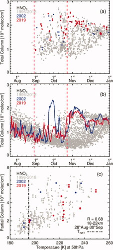
From 7^th September to 22^nd October HNO₃ measurements are variable but correlated with temperature. Figure 3 shows that the 460 K surface above AHTS remained inside the vortex. From this we infer PSCs are not present in large abundances over AHTS from 7^th September onwards. The reduction in PSCs and increased gas phase HNO₃ caused by the SSW were also observed over the Dumont D'Urville station (66.7°S, 139.8°E, 202 AMSL, ∼1500 km NW of AHTS) by Safieddine et al. (2020).

GMI HNO₃ inside the Antarctic winter vortex (Fig. 5b) is biased low in all years with less variability than the measurements. In this region and season its abundance is controlled by the PSC parameterization (Considine et al., 2000), which is tuned to approximate the denitrification and dehydration necessary to produce realistic levels of reactive chlorine, and thus may not agree with gas phase observations. On 7^th September HNO₃ increases and like the measurements, is variable and above average albeit by not as much. By 22^nd October HNO₃ has the expected steep increase. The large movement of mid-latitude airmass in 2002 is evident in the simulation. Figure 5c shows an expected positive correlation (R = 0.68) between NCEP temperature at 50 hPa (∼20 km) and HNO₃ 18-22 km partial column measurements. HNO₃ in 2002 also shows a clear correlation between temperature and abundance.

Overall, in 2019 the elevated levels of measured and modelled gas phase HNO₃ are due to the very warm stratosphere caused by the SSW. The lack of PSC’s will reduce the magnitude of heterogeneous chemical reactions by reducing chlorine activation from reservoir species. Additionally, with the returning sunlight in spring NO₂ is produced from HNO₃ photolysis (Douglass et al., 1995). With increased gas-phase HNO₃ due to renitrification we expect increased levels of reactive nitrogen (e.g. NO₂) to increase ClONO₂. We expect under such circumstances that the rate of chlorine deactivation will be greater than activation with the overall effect of reducing the rate of ozone depletion (Douglass et al., 1995; Solomon et al., 2015). In sections 5.2 and 5.3 we look at the effect of the SSW on NO₂ and the chlorine reservoirs HCl and ClONO₂.

5.2. Nitrogen dioxide (NO₂)

The usual NO₂ diurnal photochemical cycle seen at mid-latitudes becomes a seasonal cycle at the highest latitudes. With the return of spring-time sunlight NOx concentrations are initially low while most NOy resides in reservoir species HNO₃ and N₂O₅. Increasing sunlight hours towards summer lead to increased daytime NO₂. Figure 6a shows a general increase in NO₂ as daylight hours increase due to the relatively slow photolysis of N₂O₅ (Frieß et al., 2005), resulting in higher NO₂ in sunset measurements (PM 90° SZA) than in sunrise measurements (AM 90° SZA). The difference between PM and AM vertical total column NO₂ measurements are shown in Fig. 6b. These figures show a large day-night difference in 2002 and 2019. NO₂ abundances are greater at warmer temperatures in sunlit conditions (Frieß et al., 2005), compounded with increased HNO₃ abundances (Douglass et al., 1995). This is seen in Fig. 6c, where both 2002 and 2019 PM-AM differences in September (days 240-273) were anomalously high and correlated with higher than usual stratospheric temperatures. On 30^th August 2019 NO₂ PM -AM differences increase, with a large increase on 7^th September correlating directly with an associated large temperature increase. The greatest PM-AM difference, of 2.5 × 10¹⁵ molec/cm², occurs just before 17^th September coinciding with high abundances of HNO₃ and high temperatures (∼232 K). This sudden increase in NO₂ is also simulated by GMI starting on 7^th September (Fig. 6d). On 22^nd September there is a short duration (5 − 7 days) decrease in measured and modelled NO₂ correlating with a ∼20-25 K temperature decrease. A larger than normal NO₂ PM-AM difference around 17^th September was also measured at the Marambio Antarctic station (64.24°S, 56.62°W, 196 AMSL, Antarctic Peninsula) from ground-based measurements (Yela et al., 2020).

Fig. 6. (a) NO₂ total column zenith sky measurement at AHTS. Measurements are segregated into sunrise (AM) and sunset (PM). Overlaid is sunlight hours per day defined as sunrise to sunset viewed from a 20 km tangent altitude. (b) Difference between the PM and AM measurements in springtime. (c) Difference between the PM and AM measurements correlated to temperature at 50 hPA, over the period 28^th August to 30^th September (d) GMI total column NO₂ over AHTS at 1200 local time (NZST).

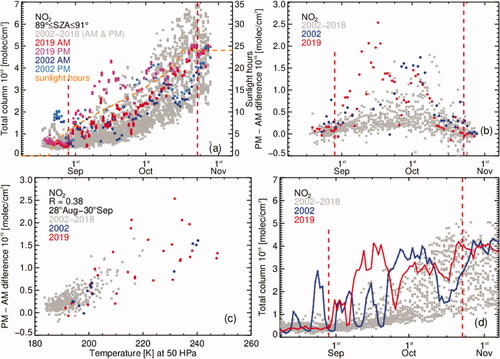
There is a rapid increase in AM NO₂ on 30^th August (red dots in Fig. 6a) from ∼0.4 × 10¹⁵ to 1.0 × 10¹⁵ molec/cm² that remains above previous years (except in 2002). This indicates not only NO_y repartitioning in favour of NO₂, but an overall increase in NO_y (renoxification) due to the increased levels of gas-phase HNO₃. Renoxification also occurred in 2002 for the same reasons along with additional mid-latitude air mixing. This has been extensively investigated by Frieß et al, 2005. High levels of reactive nitrogen will reduce heterogeneous chlorine activation as a denitrified stratosphere is a key prerequisite for chlorine activation.

5.3. Hydrogen chloride (HCl) and chlorine nitrate (ClONO₂)

HCl and ClONO₂ are chlorine reservoir species. Heterogeneous reactions convert these reservoirs to reactive species that cause large scale ozone depletion. In late winter and early spring, HCl is converted to active forms, and as the season progresses deactivation occurs and HCl starts to increase (Douglass et al., 1995; Solomon, 1999; Müller et al., 2018).

Figure 7 (a and b) shows HCl measurements and model output. In 2019, prior to 7^th September, the GMI HCl progresses within climatological norms. HCl starts increasing around 28^th August and, by the time of the first measurements (7^th September) the measured and modelled HCl are both higher than in prior years; ∼2.0-2.5 × 10¹⁵ molec/cm² compared to a mean of ∼1.5 × 10¹⁵ molec/cm².

Fig. 7. (a) HCl total column measured at AHTS. (b) GMI total column HCl over AHTS. (c) ClONO₂ total column measured at AHTS. (d) GMI total column ClONO₂ over AHTS.

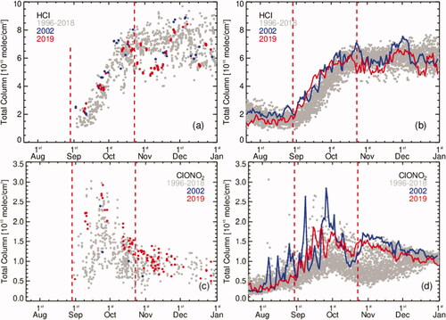
The average rate of HCl increase over the period 28^th August to 22^nd October each year (1996-2018) was 0.14 × 10¹⁵ +/- 0.03 × 10¹⁵ molec/cm²/day. In each year, the rate of increase is approximately linear. Even in 2019, with the sudden abrupt changes in stratospheric temperatures the increase was still close to linear, at a rate of 0.13 × 10¹⁵ molec/cm²/day which is within 1-sigma of the average mean rate of increase. Thus, the SSW does not seem to have significantly affected total reactive chlorine deactivation into the HCl reservoir. Under the denitrified and ozone depleted conditions typically found in late September in the Antarctic, the HCl reformation rate is controlled by Cl abundance (Douglass et al., 1995) with increased reformation rates at very low ozone mixing ratios (Grooss et al., 1997). We do not see the opposite of this, i.e. slower reformation rates at higher temperatures and ozone amounts.

The vortex edge has higher ClONO₂ concentrations compared to the vortex core due to greater concentrations and availability of reactive nitrogen species and higher temperatures (Von Clarmann, 2013), thus we expect to see more variability at AHTS since it is located close to, and underneath the vortex edge. Each year there is a seasonal spike in ClONO₂ over the period ∼7^th September to 7^th October (Fig. 7c and d). This is related to the short period in which the stratosphere is cold enough to keep chlorine activated, whilst increased sunlight hours and elevated temperatures lead to increased NO₂ abundances. ClONO₂ is rapidly formed under such conditions (Douglass et al., 1995; von Clarmann and Johansson, 2018).

Although GMI simulates the seasonal abundances well it substantially underestimates the observed late September short-lived ClONO₂ maximum. In 2019 prior to 28^th August, the GMI ClONO₂ simulations show temporal evolution as in prior years (see Fig. 7d). On the 28^th August GMI ClONO₂ increases and by 12^th September has the highest concentrations coupled with increased variability. The same is also seen in the measurements. Around 28^th August, with both chlorine reservoirs low, ClO has increased from virtually zero around 8^th August to 1.3 × 10¹⁵ molec/cm² (Fig. 8a). A single measurement on 30^th August indicates that ClONO₂ is within the climatological range (∼0.5-1.0 × 10¹⁵ molec/cm²). Eight days later (7^th September) there is large and very rapid increase in measured ClONO₂ up to 2 × 10¹⁵ from 0.5 × 10¹⁵ molec/cm². This coincides with a rapid increase in vortex temperature at 30 and 50 hPa and increased NO₂ abundances.

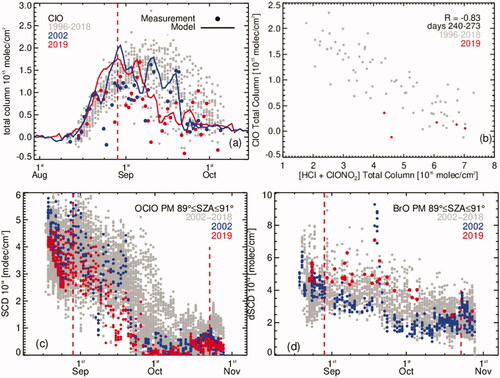
Fig. 8. (a) ClO total column (day minus night) measurements and model simulations over AHTS. (b) Scatter plot of combined HCl and ClONO2 total columns against ClO total column for the period 28^th August to 30^th September, within the polar vortex. In 2002 there is no such coincidence datasets within the vortex. (c) OClO slant column densities measured over AHTS. (d) BrO differential slant column densities measured over AHTS.

Over the period 17^th to 27^th September ClONO₂ abundances peak, corresponding with extraordinarily high temperatures and record-high levels of NO₂ a few days later. The rising temperatures release gas-phase HNO₃ from the condensed phase particles and then photolysis of HNO3 produces NO₂. This renoxification allows the reaction of ClO with NO₂ to form ClONO₂. Continuing high temperatures in the Antarctic stratosphere prohibited PSC formation, allowing higher than normal levels of ClONO₂ and NO₂ to persist up to 22^nd October. The elevated levels of ClONO₂ observed in October 2019 are not seen in 2002. ClONO₂ then slowly declines as chlorine is shifted into the longer-lived HCl reservoir (Santee et al., 2008).

Deactivation of active chlorine into ClONO₂ has not been at the observable expense of HCl reformation rate (in both 2002 and 2019). Such fast premature deactivation of active chlorine into ClONO₂ early in the Antarctic season is more akin to that seen in the warmer, and less denitrified, Arctic spring stratosphere (Douglass et al., 1995; Santee et al., 1995; Rex et al., 1997; Von Clarmann, 2013). As we will see in section 5.4 the rapid rise in ClONO₂ early in the springtime correlates with an equally fast deactivation of ClO and synchronized with an increase in temperature and NO₂.

5.4. Chlorine monoxide (ClO) and chlorine dioxide (OClO)

The ‘smoking gun’ of heterogeneous ozone depletion is ClO due to the voracious ozone destroying catalytic ClO dimer cycle (Solomon, 1999; Brasseur and Solomon, 2005). Direct measurements of ClO offer the best indicator of chlorine activation, although measurements of OClO are a good proxy (Miller et al., 1999). Measurements of ClO at Scott Base confirm the predicted strong correlations between temperature, ClO and ozone (Nedoluha et al., 2016). Seasonally, measurements and GMI simulations of ClO at AHTS peak in early September as shown in Fig. 8a. There is chlorine activation in late winter/early spring, followed by deactivation from mid spring onwards (Solomon, 1999; Nedoluha et al., 2016).

In 2019 we see ClO activation progress as in prior years up to ∼28^th August. From 28^th August to 7^th September ClO plateaus and then suddenly decreases around 7^th September. This rapid decline in ClO of ∼0.5-1.0 × 10¹⁵ molec/cm² corresponds to a similar increase in ClONO₂ abundance. From 7^th September through to 2^nd October ClO remains at record low levels, but highly variable. From 17^th September to 30^th September there is an increase in ClO correlating with decreased NO₂ and temperature. Unfortunately, there were no ClONO₂ measurements taken over this period. GMI ClONO₂ abundances show a small brief reduction over this time frame. GMI ClO peaks around 28^th August and shows a rapid decline starting around 7^th September, in line with the observed rapid decrease. In 2002 measurements and modelled ClO abundances persist longer, with a rapid decline in mid-late September coinciding with increased MPV and temperature. Observations confirm the expected strong inverse relationship (R = −0.83) between ClO and the combined chlorine reservoirs HCl and ClONO₂, as illustrated in Fig. 8b.

OClO is primarily produced through the reaction of BrO and ClO. Since the variability of reactive bromine is small compared to reactive chlorine variability, ClO is the limiting factor in OClO formation. Hence OClO can be used as an indicator of stratospheric chlorine activation (Miller et al., 1999; Wagner et al., 2001; Frieß et al., 2005) . AHTS OClO measurements are shown in Fig. 8c. These slant column density measurements show a late winter decline of OClO caused by increased sunlight since OClO is produced at night via the BrO + ClO reaction, while OClO loss occurs by photolysis. In 2019, a rapid decrease in OClO appears on 7^th September causing unseasonably low abundances coinciding with the observed decrease in ClO. There is another rapid decrease around 12^th September, followed by a short increase in OClO from 14^th September, this lasts 10 days, and is correlated with a similar short-term increase in ClO. OClO continues to decrease to near zero (or below instrument detection limits) around 27^th September. On 27^th September OClO measurements are the lowest on record for this time of year. In 2002, there is a sharp decline in OClO in mid-late September correlated with the decline in modelled and measured ClO.

There is no associated decrease in BrO (Fig. 8d) on 7^th September indicating the rapid decline of OClO is due to a reduction in ClO, not a reduction in BrO. Measured BrO remains relatively unaffected by the rapid SSW temperature and MPV changes. BrO concentrations are expected to be similar inside and outside the polar vortex (Schofield et al., 2006). BrO in 2019 is relatively high but was not duly affected by rapid temperature changes. In 2002 there is an eye-catching spike in BrO on 17^th September. Interpretation of this must be taken with care. As investigated in Frieß et al. (2005) total column BrO will be affected by tropospheric BrO plumes (aka BrO explosions, Wennberg, 1999), not related to stratospheric heterogeneous chemistry. A similar spike in BrO measurements in 2019 (coincidentally) on the 17^th September can be attributed to such a tropospheric BrO explosion event.

5.5. Ozone (O₃)

Figure 9 displays total column ozone measurements from both the ADAS2 and Dobson instruments and the GMI model. ADAS2 zenith sky measurements started earlier in the season (∼18^th August) than Dobson measurements (∼12^th September). Dobson lunar measurements are more irregular and limited to a few cloudless days each side of full moon but offer an insight to ozone concentrations during the polar night. In 2019 lunar Dobson measurements were made around 19^th July and a few over the period 8^th to 18^th September. These late winter measurements show that up to 28^th August ozone abundances are high, but within the variability seen in past years. GMI O₃ also shows this.

Fig. 9. (a) ADAS2 zenith sky total column ozone measurements over AHTS. (b) Dobson total column ozone measurements over AHTS. (c) GMI total column ozone over AHTS.

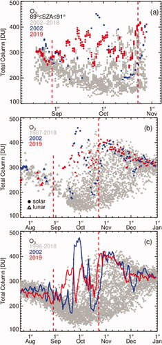
Between 28^th August and 7^th September ozone observed by ADAS2 is greater than any prior measurements made at this time of year. Higher than average ozone amounts are also simulated by GMI. Measured and modelled ozone is already above climatological levels showing the effect the SSW has even at this early stage. On 28^th August HNO₃, ClONO₂, NO₂ and ClO are also within climatological limits.

By 7^th September ozone amounts are well above seasonal averages and continue to increase, and by 12^th September ozone is above 300 DU (the seasonal mean is usually between 200 to 220 DU). By 7^th September HNO₃, NO₂ and ClONO₂ are at elevated levels along with an associated decrease in ClO and OClO.

Around 17^th September ozone levels are at an unprecedented high of 380-400 DU for springtime polar vortex air over AHTS and virtually all active chlorine has been deactivated. The only time such ozone readings were exceeded was in 2002 when there was a movement of ozone-rich mid-latitude airmasses over AHTS. Both measurements and model recorded a steep 150 DU decrease in ozone (and subsequent rebound) over the period 20^th to 30^th September 2019, correlated with a short decline and rebound in temperature (Fig. 2). This is associated with a small drop in MPV caused by the polar vortex rotating over AHTS. By 12^th October ozone levels are back within seasonal norms, at a highly variable time of year. Overall, from 28^th August through to 22^nd October ozone levels remained remarkably high. By definition, there was no ozone hole (i.e. total column ozone did not fall below 220 DU) observed at AHTS in 2019. The 2019 ozone hole was anomalously small. 2019 ozone hole metrics presented in Bodeker and Kremser (2020), shows it more akin in size, duration and severity to ozone holes observed in the 1980s.

6. Summary

We have studied the effects of the 2002 and 2019 Antarctic SSWs had on the temporal evolution of the chemical composition of the stratosphere and on ozone depletion from Arrival Heights, Antarctica. This was accomplished by using ground-based trace gas remote sensing measurements from AHTS and Scott Base along with radiosonde soundings of stratospheric temperatures from operational weather balloons launched from McMurdo Station. Serendipitously, the beginning of the 2019 SSW coincided with the arrival of the spring-time sunlight upon which the Dobson, ADAS2 and FTIR measurements depend. NCEP meteorological data and GMI chemical simulations were also used in the interpretation of the measurements.

The 2019 SSW in late winter/early spring caused an unprecedented warming of the polar vortex stratosphere. Due to the early timing of the SSW, and the fact that the warming was caused by a zonal wavenumber-1 planetary wave, the polar vortex did not split as in 2002. The vortex was displaced towards the Antarctic Peninsula until the breakup of the vortex. The end of season vortex breakup was one of the earliest on record. Unlike in 2002, the 2019 SSW caused minimal movement of mid-latitude airmasses over AHTS, this was shown by comparing the calculated MPV at AHTS and that of the vortex edge and by analysing the stratospheric tracer species HF and N₂O. These diagnostics indicate that in 2019 the evolution of reactive trace gases is explained by the stratospheric warming that affected heterogeneous chemistry, and not by dynamical mixing of mid-latitude air as in 2002.

At AHTS, the stratospheric composition remained as usual up 28^th August. By 7^th September, unusually high stratospheric temperatures exceeded the PSC formation temperature threshold and, as expected, gas-phase HNO₃ increased due to PSC sublimation. Both measurements and model results show a lack of denitrification of the stratosphere. Without permanent denitrification by sedimentation, higher temperatures allowed renoxification, as evidenced by the very large abundances of NO₂. On 28^th August we observed higher than usual HCl concentrations with ClONO₂ and ClO concentrations still within climatological norms. Up to 28^th August activation proceeded as expected as seen in the ClO levels. By 7^th September, as temperatures increased rapidly, accelerated chlorine deactivation occurred; this is seen in the decline of ClO and in OClO and an increase in ClONO₂. The decline in ClO was matched by an equal increase in ClONO₂. As stated in section 5.3, such fast premature deactivation of active chlorine into ClONO₂ early in the Antarctic season is more akin to that seen in the warmer Arctic spring stratosphere. Even though the observed chlorine deactivation pathways in 2002 and 2019 at AHTS were similar (i.e. warming leading to renitrification and increased conversion of ClO to ClONO₂) vortex dynamics were different. In 2002 the SSW brought mid-latitude air over AHTS, while in 2019 caused an increase in polar vortex air temperature.

By 17^th September chlorine deactivation was virtually complete, a record early date. From 12^th September to 12^th October there was vortex displacement away from AHTS, towards the Antarctic Peninsula while the vortex core rotated closer over AHTS during the period 22^nd to 27^th September. The effects of this were easily seen; from 12^th September to 12^th October temperatures remained extraordinarily high with large variability in gases involved in ozone depletion. Ozone levels never dropped below 220 DU at AHTS. By 12^th October, with the vortex more centred over AHTS it is too late in season for ozone depletion to restart (too warm) and from 22^nd October onwards AHTS is not underneath the vortex.

GMI simulates the observed high level of ozone over AHTS in 2019 and 2002. The movement of mid-latitude air mass over AHTS in 2002 is also captured in the simulations. GMI HNO₃ has a low bias in all years and it also does not capture the seasonal ClONO₂ maximum between 7^th and 17^th September 2019. Renoxification in 2019 and 2002 is well modelled, as seen in the elevated levels of NO₂. In 2019, GMI simulates the rapid reduction in ClO around 7^th September. Analysis, and comparison of, additional ClO data from other years is a planned activity, which will help in assessing model performance.

With the likely decrease in future satellite measurements of the stratosphere (Fussen et al., 2019; Hegglin et al., 2020), the unique long-term suite of measurements at AHTS will become increasingly critical to our monitoring of the Antarctic stratosphere. The measurement suite on Ross Island can be expanded and improved. A harmonized time series of the radiosonde temperature dataset would allow robust decadal trend analysis and traceability. Such an activity is underway through GRUAN. To tell a clearer story, PSC and stratospheric water vapour measurements are needed. A Fe-Boltzmann Rayleigh lidar (Chu et al., 2011) was installed at AHTS in 2010 and it has the potential to detect PSCs (Dr Xinzhao Chu, personal communication, July 30, 2019). Additionally, UV/Vis zenith sky measurements have the potential to detect PSCs (Sarkissian et al., 1991) and we plan to investigate the possibility of applying this technique to ADAS2 spectra. A handful of GRUAN compliant frost point hygrometer soundings (Vömel et al., 2007; Müller et al., 2016) to measure stratospheric water vapour are planned at Scott Base in the 2021-2022 summer season to see if monthly flights are logistically feasible in the long term.

Acknowledgements

We would like to thank NIWA meteorologists Ben Noll and Nava Fedaeff for suppling Fig. 1 along with discussions concerning the meteorology of the 2019 SSW event, Antarctica New Zealand for providing logistical support for the measurements at Arrival Heights and Scott Base, and the McMurdo USAP weather forecasting team.

We appreciate the support of the University of Wisconsin-Madison and Madison College AMRDC for the use of the radiosonde data set, NSF grant numbers 1924730 (UW) and 1951603 (MATC).

Disclosure statement

The authors declare that there are no conflicts of interest regarding the publication of this article.

Additional information

Funding

Measurements at Arrival Heights and Scott Base are core‐funded by NIWA through New Zealand's Ministry of Business, Innovation and Employment Strategic Science Investment Fund. The ClO measurements at Scott Base are supported by the NASA Upper Atmosphere Research Program