A review on restoration of seismic wavefields based on regularization and compressive sensing

Abstract

Restoration of seismic data as an ill-posed inverse problem means to recover the complete wavefields from sub-sampled data. Since seismic data are typically sparse in the curvelet domain, this problem can be solved based on the compressive sensing theory. Meanwhile three major problems are modelling, sampling and solving methods. We first construct l₀ and l₁ minimization models and then develop fast projected gradient methods to solve the restoration problem. For seismic data interpolation/restoration, the regular sub-sampled data will generate coherence aliasing in the frequency domain, while the random sub-sampling cannot control the largest sampling gap. Therefore, we consider a new sampling technique in this article which is based on the controlled piecewise random sub-sampling scheme. Numerical simulations are made and compared with the iterative soft thresholding method and the spectral gradient-projection method. It reveals that the proposed algorithms have the advantages of high precision, robustness and fast calculation.

Keywords:

• wavefield recovery
• curvelet transform
• compressive sensing
• inverse problems
• ill-posedness
• projected gradient method

AMS Subject Classifications::

• 65J22
• 86A22

1. Introduction

In exploration seismology, the process of acquisition records the continuous wave field which is generated by the source. In order to restore the seismic data correctly, the acquisition should satisfy the Nyquist/Shannon sampling theorem, i.e. the sampling frequency should at least be twice the maximum frequency of original signal. In seismic acquisition, because of the influence of obstacles at land surface, rivers, bad receivers, noise, acquisition aperture, restriction of topography and investment, the obtained data usually does not satisfy the sampling theorem. A direct effect of the limitations of acquisition is that the sub-sampled data will generate aliasing in the frequency domain; therefore, it may affect the subsequent processing such as filtering, de-noising, AVO (amplitude versus offset) analysis, multiple eliminating and migration imaging. In order to remove the influence of sub-sampled data, the seismic data restoration/interpolation technique is often used. On the other hand, seismic data interpolation can generate high-resolution data which will save the cost and improve the imaging results. In summary, seismic data restoration is an important research direction in exploration seismology 1,2.

Many seismic data restoration methods have been developed in the past few years. Mostafa and Sacchi 3, classify the methods for seismic wavefield recovery into two kinds: wave-equation-based methods and signal processing methods. According to our knowledge these methods can be classified into four classes. The first class is the prediction error filter methods. Seismic data can be obtained by finding a convolution filter that predicts the data in such a way that the error is white noise. The well-known f–x predictive method in 4,5 can restore the spatially aliased regularly sub-sampled data. The low-frequency data components are utilized to recover the high-frequency data. A modified projective prediction error filter method was proposed in 6. However, these methods are applicable only if the original data is regularly sampled in space and will cost a lot in computation. Similar methods in the f–k domain 7 for band-limited signals use the Fourier transform to predict the complete wave field. The interpolation method that rely on the t–x domain predictive filters were introduced in 8–10, which first estimate the dip in a sliding time window and then interpolate along the dip direction in each time window. All the above-mentioned methods are based on the assumption of linear events; the restoration will deteriorate for cross events. The second kind of method is based on the wave equation. These methods utilize the physical properties of wave propagation to restore seismic data. An integral with a continuous operator is often used to obtain the complete wave field 11,12. Some information of velocity distribution in the interior of earth is needed for these methods. The third class is the mathematical interpolation in the time domain. These methods include sinc interpolation after alias reduction via NMO (normal movement) correction 13, most coherent dip interpolation 14, interpolation using event attributes and power diversity slant--stack interpolation. The sinc interpolation methods are not appropriate for far offset data, while the most coherent dip interpolation is only suitable for data consisting of linear events. The last kind of method is based on the Fourier analysis. Some a priori knowledge such as the seismic signals being band-limited or sparseness of seismic data is needed. The seismic data are decomposed through a transform. These methods are robust for noisy data. Methods based on Fourier transform 15–19 can be applied to seismic signals with spatially band-limited property. The methods based on linear Radon transform 20 and parabolic Radon transform 21 can focus the energy of signals in the transformed domain. The curvelet transform was introduced in seismic restoration in 22,23, and was proved to be the most sparse one for seismic data.

The model of seismic acquisition can be written as (1) where A ∈ ℝ^l×m is the sampling operator, x ∈ ℝ^m is the reflectivity model, and b ∈ ℝ^l denotes the sampled data. The restoration problem is to solve x from A and b, thus it is an inverse problem. A problem is called well-posed if the solution of (1) exists, is unique and continuous. If any one of these conditions is violated, the problem is ill-posed. Equation (1) can be solved by finding a least squares solution, i.e. solving the problem (2) where ‖ · ‖₂ is the Euclidean norm of a vector. It is equivalent to solving the normal equation (3) where A^T is the transpose of A. However, the direct inversion of (3) produces an unstable solution. In order to obtain a stable solution, regularization is necessary.

A popular method for solving ill-posed problems is the Tikhonov regularization, which refers to solving a regularized functional (4) where Ω(·) is the so-called Tikhonov stabilizer and α > 0 is the regularization parameter. We often choose , where D is a positive semi-definite and bounded operator. Then, the minimizer of J_α(x) is given by (5)

For solving Equation (5), several methods such as LU decomposition, singular value decomposition and QR decomposition can be used 24. However, any direct method should be avoided and iterative solvers are preferred for geophysical inversion problems. The commonly used iterative methods involve conjugate gradient-type methods, Newton-type methods and statistical methods based on Bayesian inference 24. However, these methods may be time consuming and other methods which possess fast convergence and stability are desirable for large-scale seismic data restoration problems.

For seismic interpolation problem, let us denote by x the original seismic wave field, b the sampled data and A the sampling operator, the expression again can be written as (1). Our purpose is to restore x from the sampled data b. Since b is usually incomplete, A is an under-determined operator. This indicates that there are infinite solutions satisfying the seismic interpolation Equation (1). Hence, seismic data interpolation is an ill-posed inverse problem.

The compressive sensing in information theory could be used to recover the original data from insufficient sampling, which breaks the limitations of the Nyquist/Shannon sampling theorem. This theory has been applied in many application fields. Theoretically, if the seismic data is sparse under a transform, then we can restore the complete data from sub-sampled data according to the compressive sensing. Another potential application of the compressive sensing theory in seismology is the design of new sampling methods in seismic acquisition. As we all know, seismic acquisition expends a lot of time and money. The number of sources and receivers can be reduced greatly based on compressive sensing, which will save the acquisition cost. At the same time, the complete wave field can still be recovered from partial sampled data.

Finding the sparse solution of an under-determined system is also a crucial issue in seismic processing. Due to huge storage of the data volume and the specific sampling, methods for solving general problems cannot be used in seismic data restoration directly. So far, developed methods include the iterative soft thresholding method 25,26, the spectral projection-gradient method 27 and the iterative re-weighted least squares method 28. However, these methods do not converge very fast which may lead to deficient usage.

It is well-known that the best model for finding a sparse solution of an under-determined system is the solution in l_q space with q → 0. Therefore, to meet the above requirements of applying compressive sensing to seismology, we consider the smoothing l₀ method and develop two fast and robust algorithms for solving the sparse restoration problem. As far as we know, the methods we consider have not been addressed in the literature for restoration of seismic wavefields.

The outline of this article is as follows. We give a short review of the concept of compressive sensing in Section 2.

In Section 3, we introduce the sparse transform. In particular, the popular curvelet transform is introduced. As a multi-scale, multidirectional, anisotropic and local transform, it has great advantages over the Fourier transform, Radon transform and the wavelet transform for seismic data processing. Therefore, it can be used in seismic data recovery.

Our recently developed sampling scheme 2 for seismic restoration is introduced in Section 4. Random sub-sampling cannot control the largest sampling gap which is unfavourable for curvelet-based wave field restoration 25, and the regularly sub-sampled data will generate aliasing in the frequency domain. Our sampling technique can both control the sampling gap and reduce the aliasing in the frequency domain. It is worthwhile to mention that a lot of sampling methods were proposed in different applications, but they cannot be introduced directly to solve seismic restoration because of the specialty of seismic acquisition.

In Section 5, we first give a brief review of the classical methods, and then we devote ourselves to build the l_q model with q = 0 and q = 1 and develop two fast and robust methods for solving the sparse restoration problem.

Numerical simulations are given in Section 6. In Section 6.1, we show that our controlled sampling method can greatly improve the restoration; its performance is comparable with the jittered sampling 22. In Sections 6.2 and 6.3, we show that our proposed methods based on l_q model with q = 0 and q = 1 along with our sampling technique are fast and robust in sparse restoration of seismic wavefield. In Section 6.4, a field data example is presented. The performance of different methods for the practical data are compared. Some remarks on classical matching pursuit and orthogonal matching pursuit methods are addressed in Section 6.5. Finally in Section 7, we discuss the potential usage of the compressive sensing and other interesting study fields.

2. The basics of compressive sensing

The Nyquist/Shannon sampling theorem as the foundation of digital signal and image processing is widely used in many areas. But it takes a lot of time in computation and storage since the amount of sampled data is huge. Because of the restriction of sampling time and sampling numbers in applications, the sampled data usually disobey this theorem. Therefore, it is necessary to find new sampling methods to break the restriction.

If the sampling process is linear, then it can be written as (6) where f ∈ ℝ^N is the original signal, b ∈ ℝ^M is the sampled data and Φ ∈ ℝ^M×N is the sampling matrix. If the sampled data is incomplete, i.e. M < N, then Equation (6) is under-determined. This indicates that inversion of (6) is ill-posed.

The recently posed compressive sensing theory can restore the original data from the sub-sampled data. However, this theory is based on two basic conditions. First, the original signal f must be sparse under some transform, i.e. f can be expressed as f = Ψs, where s has a few non-zero entries. The Fourier transform is commonly used in signal processing, and signals are usually decomposed in the frequency domain. The discrete cosine transform and wavelet transform are two famous transforms for signal/image processing. The wavelet transform can also be used to restore a medical image using magnetic resonance imaging (MRI) 29. For seismic data processing, the commonly used transforms include the Fourier transform 17,18, the linear Radon transform 20, the parabolic Radon transform 21 and the Gabor transform. If there exists a transform Ψ such that s = Ψ^Tf is sparse, then Equation (6) can be changed into (7) where A = ΦΨ. Another condition for compressive sensing is that A must satisfy the restricted isometry property (RIP) 30,31. If Φ is the Gaussian random matrix, the partial Fourier matrix, the uniform spherical matrix, the binary random matrix, the partial Hadamard matrix or the Toeplitz matrix, then A satisfies the RIP. If K < C · M/log(N/M), the sparse solution can be solved, where C is a universal constant and K the number of non-zero elements of s 31.

If the above two conditions are satisfied, we can find s by solving Equation (7), which is actually an optimization problem (8) where ‖·‖₀ denotes the number of non-zero entries. As a combinatorial optimization, solving this problem essentially requires exhaustive searches over all subsets of columns of A 30,32.

3. Sparse transforms

3.1. Transform classification

Sparse transform is an important part of compressive sensing. If the coefficients in the transform domain are very sparse, then only small sampling numbers are enough. In the seismic processing, the most commonly used transforms are the Fourier transform, the linear Radon transform, the parabolic Radon transform and the curvelet transform. The linear Radon transform can focus the energy of linear events; the parabolic Radon transform can compress events with parabolic shapes. Although applications of wavelets have become increasingly popular in scientific and engineering fields, traditional wavelets perform well only at those points which possess singularities, and the geometric properties, e.g. waveforms of wave fronts in seismic data are not utilized. The ridgelet transform can deal with the linear events, but fail with curve events. Curvelet transform as a multi-scale ridgelet transform, and is multi-scale, multi-directional, anisotropic and local 33. Curves are approximated by piecewise line segments in the curvelet domain; therefore, seismic signals can sparsely be compressed.

3.2. The curvelet transform

Similar to the wavelet and ridgelet transforms, curvelet transform can be represented by inner product of the curvelet functions ϕ and the signal f(x) (9) where f ∈ L²(ℝ²), ϕ_j,l,k denotes curvelet function and is the conjugate of ϕ, which is indexed by three parameters: a scale parameter 2^−j, j ∈ ℕ₀ (ℕ₀ is the positive integer set), a sequence of rotation angles θ_j,l = 2πl · 2^−⌊j/2⌋, 0 ≤ l ≤ 2^−⌊j/2⌋ − 1 and a position (ℤ denotes the integer set), where is the rotation matrix with angle θ_j,l. Curvelets consist of directional entries ϕ_j,l,k(x) in fine scales and isotropic entries in coarse scales. In fine scales, the curvelet function can be written as (10) while in coarse scales, the curvelet function can be denoted as , which indicates that the curvelets are isotropic in the coarse scale. The function ϕ_j(x) is the waveform by means of its Fourier transform , which serves as a ‘mother’ curvelet in the sense that all curvelets at scale 2^−j are obtained by rotations and translations of ϕ_j. Numerical implementations of curvelet transform can be outlined in three steps: applying 2D FFT, product with frequency windows and applying 2D inverse FFT for each window. Through the curvelet transform, the original signals are decomposed into various scales and angles. Its discrete form can be written as c = Sf, where c is a vector denoting the discrete set of curvelet coefficients, f is the discrete form of the data and S = W_FF₂ is the curvelet transform matrix, where F₂ is the 2D Fourier transform matrix and W_F denotes the windowing operator followed by 2D inverse Fourier transform in each scale and in each direction. The computational cost of the forward and inverse curvelet transform is 𝒪(N² log N) for an N × N data. We refer to 34,35 for details of the implementation of the curvelet transform by involving FFT and IFFT. The inverse curvelet transform can be written as f = S*c, where S* denotes the adjoint operator of S. Since seismic data are sparse under the curvelet transform, we use it as the sparse transform in this article.

4. Sampling

The sampling technique is important for compressive sensing. It is closely related to the quality of restoration, e.g. correct sampling in MRI and radar imaging 29 can improve the quality of restoration. In seismology, because the receivers can only receive the signals on the ground, traditional sampling methods cannot be employed in seismic exploration directly. There are mainly two sub-sampling methods: the regular sub-sampling and the random sub-sampling. In the former, the receivers are located at equal distance, but they may not satisfy the Nyquist/Shannon theorem. A direct consequence of the regular sub-sampling is the coherent aliasing which is not straightforward for transform-based restoration and is difficult to remove. In the random sub-sampling, the receivers are placed randomly on the survey line. The aliasing caused by random sub-sampling in the frequency domain can be seen as random noise, thus the restoration problem can be treated as a de-noising problem 25. If the gap size of random sampling is large, the recovered data will lose some information. Therefore, a sampling method which can control the gap size and preserve the randomness is necessary for seismic restoration.

The jittered sub-sampling proposed in 22 can both control the gap size and preserve the randomness, so it is better than the random sampling. However, this method is not flexible. In view of these sampling methods, a piecewise random sampling method, developed by us recentley, will be utilized. This sampling technique can both control the gap size and keep the randomness and is flexible. For the random sampling, the probability of been sampled is the same for each position. If the Nyquist sampling number is N, and the actual chosen number is K, then the largest gap may be N − K. If the gap size is larger than the scale of the curvelet, then some information cannot be restored. Instead, if the N positions are first divided into M pieces, the length of each piece is N/M, and random sampling with the ratio of K/N is in each piece, then the largest gap size is 2(N/M)(1 − K/N), therefore, the gap size is controlled. And at the same time, the randomness is also retained.

The piecewise sampling method can be described as follows: (i) divide the N positions into M pieces, where the length of each piece N/M should be less than a scale of the curvelet; (ii) randomly choose K/M positions at each piece, thus the total sampling number is K. If the number of pieces being divided is large enough, then the gap size is small. Thus, it will improve the quality of restoration.

It deserves attention that in a recent work, Naghizadeh and Saachi 23 succeed in reconstructing regularly decimated aliased seismic data based on choosing a special mask function. This method relies on choosing a user-defined threshold or a nearest neighbour operator. Although additional effort is added, it is a promising sampling method.

5. Methods of solution

5.1. Classical methods

Finding the sparse solution of under-determined problems has been studied in many areas, meanwhile the commonly used methods are based on the l₁ norm optimization. These methods find the sparse solution by solving (11) where ‖ · ‖₁ denotes the l₁ norm. This problem can be changed into linear programming, and then solved by interior point methods 1,36–38. Suppose that the sampling process has additive noise n, we obtain b = As + n; therefore, the corresponding problem becomes (12) where ε is a nonnegative real parameter which controls the noise level in the data. This problem can be solved as a second-order cone program. Problems (11) and (12) are closely related to the following two problems: (13) and (14) where λ is the Lagrange multiplier. With appropriate parameter choices of ε, λ and δ, the solutions of (12), (13) and (14) coincide, and these problems are in some sense equivalent.

A lot of methods can be used to solve problems (11–14). The homotopy method was originally designed for solving noisy over-determined l₁-penalized least squares problems 39. It was also used to solve under-determined problems in 40. This method for the model problems (11–14) has been considered in 41,42. The least angle regression method as a modification of the homotopy method, considered in 43, was investigated solving problem (14). When the solution is sufficiently sparse, these two methods are more rapid than general-purpose linear programming methods even for the high-dimensional cases. If the solution is not rigorously sparse, the homotopy method may fail to find the correct solution in certain scenarios.

Another popularly used method is the interior point method. In 1, an interior point method based on equality and inequality constraints are addressed. In 38, problems (11) and (13) are solved by first reformulating them as ‘perturbed linear programs’, then applying a standard primal-dual interior point method. The linear equations are solved by iterative methods such as LSQR or conjugate gradient method (CGM). Another interior point method given in 44 is based on changing (13) into a quadratic programming (QP) problem solved by preconditioned CGM. Problem (12) can also be solved by reconsidering it as a second-order cone programming and then applying a log-barrier method, e.g. methods developed in 36,45 are used to solve the land surface parameter retrieval problems.

Iterative soft thresholding methods were used to solve problem (13) 46. But they are sensitive to the initial values and are not always stable. In addition, many iterations are required for convergence.

Recently, the spectral gradient-projection method was developed for solving problem (12) 27. The method relies on root-finding of the parameter δ by solving the non-linear convex, monotone equation ‖As(δ) − y‖₂ = ε. This method can handle both noisy and noiseless cases. However, it is clear that the root-finding method is the famous ‘discrepancy principle’ in regularization theory for ill-posed problems 47.

Matching pursuit (MP) and orthogonal matching pursuit (OMP) 48–50 are also used for sparse inversion. This is known as a kind of greedy approach. The vector b is approximated as a linear combination of a few columns of A, where the active set of columns to be used is built in a greedy fashion. At each iteration, a new column is added to the active set. OMP includes an extra orthogonal step which is known to perform better than the standard MP. The computational cost is small if the solution is very sparse. However, only small dimensional problems are suitable for these methods. If Ax = b, with x being sparse and the columns of A being sufficiently incoherent, then OMP finds the sparsest solution. It is also robust for small levels of noise 49.

The projected gradient method developed in 51 express (13) as a nonnegative constraint quadratic programming by separating s as s = (s)₊ − (−s)₊, where (s)₊ = max{s, 0}. However, this method can only tackle real numbers, thus it is unsuitable for curvelet-based seismic data restoration. The iterative re-weighted least squares method developed in 52 changes the weights of entries of s at each iteration. A similar method was proposed in 53.

Methods based on non-convex objects are studied in 54,55. In 54, the l₀ norm is replaced by a non-convex function. However, initial values must be carefully chosen to prevent the local optimal solution. Other methods such as iterative support detection method 56 and fix point method are also developed.

As an inverse problem with a priori knowledge the above problems fall into the general l_p − l_q model 57: (15) Regularizing active set (projection) method can be applied.

These methods have extensive applications in various fields, such as image reconstruction, MRI 29, seismic images 22, model selection in regression 43 and texture/geometry separation.

5.2. Two fast methods for seismic restoration

Usually, the seismic restoration is a large-scale problem, thus fast solving methods are crucial for seismic processing. Because of the large dimension of seismic data, traditional methods such as interior methods 38, homotopy methods 40 and least angle regression methods 43 cannot be used to large-scale seismic restoration. The iterative soft thresholding (IST) method was introduced to recover the seismic data in 22. A robust spectral gradient-projection (SPGL1) method was proposed in 27 to solve problem (14). In 58, the iterative re-weighted least squares was used for interpolation. Unfortunately, these methods have slow convergence rate for large-scale problems 59, therefore, it is urgent to find fast convergent methods.

We develop two fast methods for seismic restoration in this section. They are very fast compared with the above three methods. The CPU time takes only about 1/3 of the SPGL1 method, and about 1/4 of the IST method. Numerical experiments in Section 6 verify the quick convergence of the developed methods.

5.2.1. A smooth l₀ method

The original problem for l₀ minimization is the following equality constrained optimization problem: (16) However, direct solution of (16) is hard to obtain because it is time consuming. Obviously, solving the true l₀ norm optimization is superior to the l₁ norm optimization though both methods can yield sparse solutions. We consider approximation of l₀ minimization problem. Denote f_σ(t) = 1 − exp(−t²/(2σ²)) as a function of σ and t. This function satisfies the following properties: (a) f_σ(t) is continuous and differentiable; (b) f_σ(t) tends to the l₀ norm when σ tends to 0, i.e. (17) Thus, we can construct a continuous function to approximate the l₀ quasi-norm, and then obtain the optimal solution. In this way, problem (16) is approximated by (18)

The object function J_σ(x) is differentiable and is closely related to the parameter σ: the smaller the value of σ, the closer the behaviour of J_σ(x) to the l₀ quasi-norm. For small values of σ, J_σ(x) is highly non-smooth and contains a lot of local minima, hence its minimization is not easy. On the other hand, for larger values of σ, J_σ(x) is smoother and contains fewer local minima, and its minimization is easier. Practically, we use a decreasing sequence values of σ: for minimizing J_σ(x) for each value of σ, the initial value of the minimization algorithm is the minimum of J_σ(x) from the previous value of σ. Then we apply a simple projected gradient method to solve Equation (18). Details of the procedure are given in Algorithm 1. For the convergence of a similar method for general signal processing problems, we refer to 54 for details. Below we present a similar algorithm to 54 based on the above l₀ norm approximation and use it for seismic wavefield restoration.

Algorithm 1 (Smooth l₀ method)

1.	Initialization: 1. Let be the minimum l2-norm solution of Ax = b, which can be obtained by applying the pseudo-inverse of A. 2. Choose the inner loop number L, outer loop number J and the step-length τ; set a decreasing sequence values of σ : [σ1, … , σJ].
2.	Iteration: for j = 1, … , J 1. Let σ = σj. 2. Minimize the function Jσ(x) on the feasible set 𝒮 = {x|Ax = b} using L iterations of gradient descent method. ① Let ; ② For l = 1, … , L: a. Let gσ = [∇Jσ(x1), ∇Jσ(x2), … , ∇Jσ(xn)]. b. (The gradient decent iteration): x = x + τd (τ is the step-length, d = γ(gσ)). c. (Projection): Project x on the feasible set 𝒮 = {x|Ax = b}: 3. Set , σ = σ/2.
3.	Final solution is .

We can also choose other functions to approximate the l₀ quasi-norm, e.g. the ‘truncated hyperbolic’ function: (19) and (20)

Remark 1

In Step 2 of Algorithm 1, if the gradient descent step is based on steepest descent (SD) step, i.e. γ(g_σ) = −g_σ and τ = τ^SD, then the algorithm corresponds to projected steepest descent method.

In addition, in Algorithm 1, the inner loop number L need not be too large, and according to our experience, the step-length τ should be greater than 2 to ensure fast convergence. However, it is clear that this choice of the step-length is not optimal. Usually, we need to calculate an optimal step-length τ* by line search for the one-dimensional problem τ* = argmin_τ J_σ(x + τd). One may readily see that some fast gradient methods based on non-monotone gradient descent step can be applied, e.g. the Barzilai--Borwein step used in seismic migration inversion 60, where the function γ(g_σ) is updated by the former iterative information instead of the current iterative information.

For curvelet-based restoration, because of the orthogonality of the curvelet transform, the inverse of AA^T is the identify matrix, thus the projection onto 𝒮 = {x|Ax = b} can be simply solved by x = x − A^T(Ax − b).

5.2.2. Approximations of the l₁ norm optimization

As it is well-known that the objective function based on l₁ norm is non-differentiable at the original point, most of the solvers for l₁ norm optimization are based on the interior point methods to solve a linear programming problem. In this section, we consider using smooth functions to approximate the l₁ norm. We consider the function (21) which is continuous, convex and differentiable. If ε is small enough, f_ε(t) will approximate the l₁ norm sufficiently, thus it can be used to replace the l₁ norm 24. Another similar function is (22) If θ is large enough, then f_θ will approximate the l₁ norm. This function has been used for solving non-linear and mixed complementarity problems and feature classification 61,62.

Since the object function based on f_ε(t) or f_θ(t) is an approximation of the l₁ norm, the errors are inevitable. However, the cost of computation will be much less than the IST method and SPGL1 method. At each iteration of the SPGL1 method, one needs to project the iteration point to the active set specified by the l₁ norm, which will increase the amount of computation 27; while the gradient projection for sparse reconstruction (GPSR) method cannot deal with complex numbers 51. We found that the smaller the values of ε, the better the approximation of f_ε(t) to the l₁ norm; the smaller the values of θ, the worse the approximation of f_θ(t) to the l₁ norm. Thus, we can solve the following problems to get the sparse solution: (23) or (24)

We use a projected gradient algorithm to solve these two problems. Details are outlined in Algorithm 2. In our algorithm, a projection to 𝒮 = {x|Ax = b} is also needed. However, the projection is easy to be computed. Since A is orthogonal, the initial l₂ norm solution can be obtained by x = A^Tb, and the projection can be easily calculated through . However, it is different from the smooth l₀ algorithm because it does not need the outer iteration.

Algorithm 2

(Projected gradient method for approximation of the l₁ norm optimization)

1.	Initialization: 1. Choose the maximum loop number L, set ε = 1.0e − 16 (or θ = 1000), and k = 0. 2. Let x0 be the l2 norm solution of Ax = b, which can be obtained by the pseudo-inverse of A.
2.	Iteration: 1. Let gε = ∇Fε(xk) (or gθ = ∇Fθ(xk)). 2. Perform the gradient decent iteration: (τ is the step length, d = γ(gε) or d = γ(gθ), denotes the predicted step). 3. Projection: Project on the feasible set 𝒮 = {x|Ax = b}: 4. Let xk = xk+1, k = k + 1.
3.	Final solution is x = xL.

In Step 2 of Algorithm 2, if the gradient descent step is based on steepest descent step, i.e. γ(g_ε) = −g_ε or γ(g_θ) = −g_θ and τ = τ^SD, then the algorithm corresponds to projected steepest descent method. More advanced choices of the function γ and the step-length τ are given in Remark 1.

6. Numerical examples

6.1. Piecewise sampling vs. random sampling

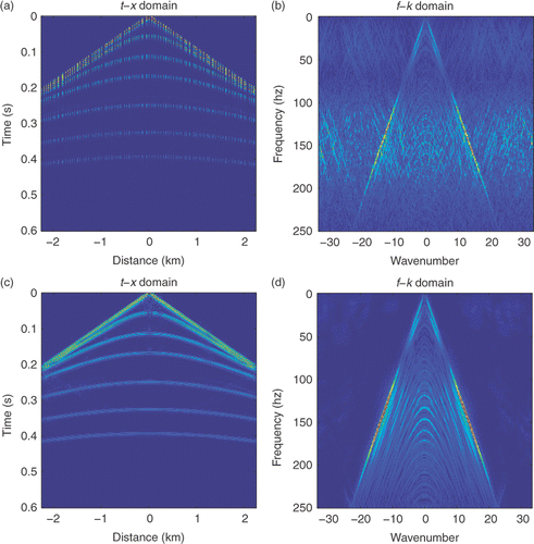
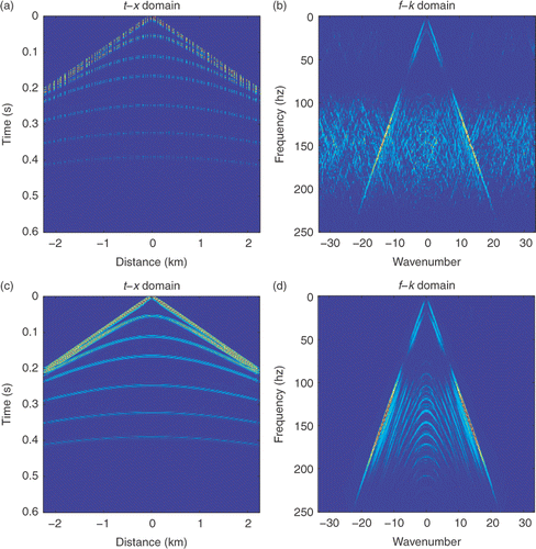
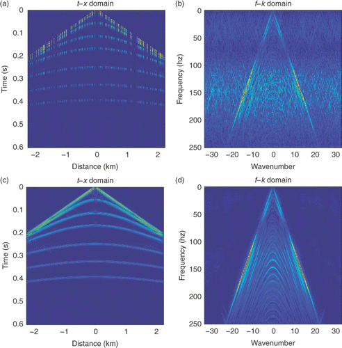
Considering a synthetic shot data of a layered earth model with six plane layers, modelled with a 15 m receiver interval, 2 × 10⁻³ s sampling interval and a source function given by a Ricker wavelet with a central-frequency of 15 Hz. The dataset contains 256 traces of seismic data with 256 time samples in each trace. The original shot gather and its frequency spectrum are shown in Figure 1(a) and (b). The resulting shot gather after regular sub-sampling and its corresponding frequency spectrum are shown in Figure 1(c) and (d). In this simulation, the sampling number is 1/3 of the Nyquist sampling number. Serious coherent aliasing can be seen in Figure 1(d). With the same number of regular sampling, the random sampling and its frequency spectrum are shown in Figure 2(a) and (b). It reveals that the aliasing in Figure 2(b) is just like random noise; the recovery results by SPGL1 and the corresponding frequency spectrum are given in Figure 2(c) and (d). To show the degree of restoring ability, we adopt the signal-to-noise ratio (SNR) defined by . The SNR using the random sampling is about 7.1606, where data_orig denotes the complete data and data_rest denotes the recovered data. With the same number of regular sampling, the jittered sampling and its frequency spectrum are shown in Figure 3(a) and (b); the restoration and the restored frequency spectrum are given in Figure 3(c) and (d). The SNR using the jittered sampling is 9.3008. We also perform our piecewise sampling simulations. The piecewise sampling and its frequency spectrum can be seen in Figure 4(a) and (b); the restoration results and the restored frequency are shown in Figure 4(c) and (d). The SNR of restoration using the piecewise sampling is 9.8417. The numerical performance indicates that the piecewise sampling can improve the restoration greatly.

Figure 1. (a) The original data and (b) its frequency; (c) the regular sub-sampling and (d) the frequency of the sub-sampled data.

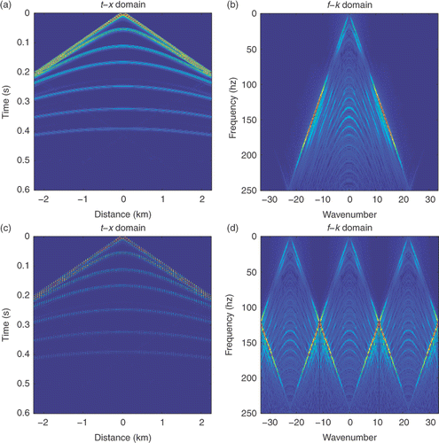
Figure 2. (a) The random sampling and (b) its frequency; (c) the restoration results and (d) the frequency of the restored data.

Figure 3. (a) The jittered sampling and (b) its frequency; (c) the restoration results and (d) the frequency of the restored data.

Figure 4. (a) The piecewise sampling and (b) its frequency; (c) the restoration results and (d) the frequency of the restored data.

6.2. Results of the smooth l₀ method

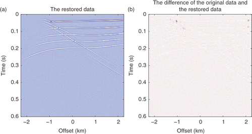
We give examples to show the superiority of the smooth l₀ method to the IST and SPGL1 methods. The synthetic data consists of 300 traces with spacing 15 m. The temporal sample interval is 2 × 10⁻³ s and the sampling number is 300. The full data and the incomplete acquisition are depicted in Figure 5(a) and (b), respectively, where the sampling number in Figure 5(b) is half of the Nyquist sampling number. The restoration results by the smooth l₀ method and the difference between the restoration and the original data are shown in Figure 6, where we choose f_σ(t) = 1 − exp(−t²/(2σ²)). The restoration results by the smooth l₀ method using the approximate function f_σ(t) = 1 − σ²/(t² + σ²) and difference between the restoration and the original data are given in Figure 7(b). Similar results of smooth l₀ method using the approximate function are shown in Figure 8. The restoration results by the IST method and the difference between the restoration and the original data are shown in Figure 9. While the results using the SPGL1 method are shown in Figure 10. Table 1 summarizes details of the SNR, the relative error and the cost of computation of these methods. The results show that the smooth l₀ method is much faster than the IST and SPGL1 methods. It uses the CPU time about 1/4 of the IST method, and about 1/3 of the SPGL1 method to yield the similar results. Thus, we conclude that the smooth l₀ method is suitable for seismic data restoration.

Figure 5. (a) The original data; (b) the sampled data with randomly removed half of the receiver positions.

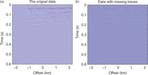
Figure 6. (a) Restoration results by the smooth l₀ method with f_σ(t) = 1 − exp(−t²/(2σ²)); (b) the difference between (a) and the original data.

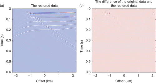
Figure 7. (a) Restoration results by the smooth l₀ method with f_σ(t) = 1 − σ²/(t² + σ²); (b) the difference between (a) and the original data.

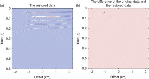
Figure 8. (a) Restoration results by smooth the l₀ method with ; (b) the difference between (a) and the original data.

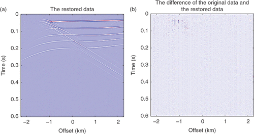
Figure 9. (a) Restoration results by the IST method; (b) the difference between (a) and the original data.

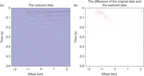
Figure 10. (a) Restoration results by the SPGL1 method; (b) the difference between (a) and the original data.

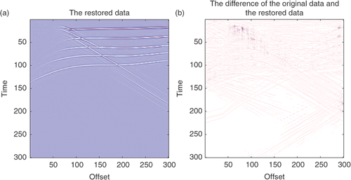
Table 1. Comparison of the smooth l₀ method, IST method and the SPGL1 method.

Algorithm		SNR	Relative error	Time (s)
Smooth	l0 with fσ(t) = 1 − exp(−t^2/(2σ^2))	25.5282	0.0529	306
Smooth	l0 with fσ(t) = 1 − σ^2/(t^2 + σ^2)	25.6524	0.0522	318
Smooth	l0 with	23.6445	0.0657	323
IST		24.8597	0.0571	1326
SPGL1		25.1210	0.0555	1069

6.3. Results of the l₁ norm optimization using projected gradient methods

We use the same full data and sampled data as in Figure 5 and perform Algorithm 2. The number of sampling is half of the Nyquist number. When the l₁ norm is replaced by F_ε(x), where ε = 1.0e − 20, then after 30 iterations, the SNR of the restored results approaches 22.8120 and the CPU time is 229 s. The restoration results and the difference between the restoration and the original data are shown in Figure 11. When F_θ(x) is used to replace the l₁ norm, where θ = 1000, then after 30 iterations, the SNR approaches 23.2334 and the CPU time is 241 s. The restoration results and the difference between the restoration and the original data are shown in Figure 12. It is evident that both the convergence rate is fast and the solution is acceptable. Though the restoration has random noise, the key information can still be restored; therefore, this method can be applied to seismic data restoration. However, to better apply this method to seismic data processing, the next major work is to remove the random noise. Some tricks may be used: (i) normalization of the original data, which will lead to small coefficients in the curvelet domain; (ii) since curvelet coefficients are focused on the first half of the vector, the latter half part of vector can be truncated to boost the SNR.

Figure 11. (a) Restoration results using F_ε(x) to replace the l₁ norm; (b) the difference between (a) and the original data.

Figure 12. (a) Restoration results using F_θ(x) to replace the l₁ norm; (b) the difference between (a) and the original data.

6.4. Field data applications

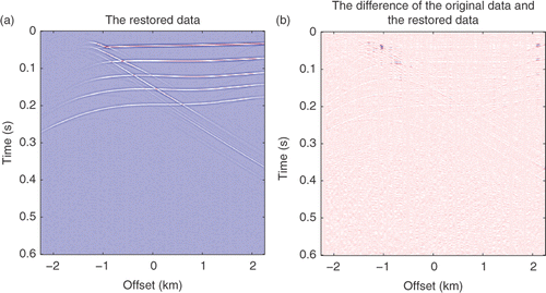
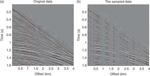
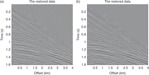
We further examine the efficiency of the new methods with field data. A marine shot gather is provided in Figure 13(a) which consists of 160 traces with spacing 25 m and 800 time samples with interval 2 × 10⁻³ s. There are damaged traces in the gather. The sub-sampled gather is shown in Figure 13(b) with half of the original traces randomly deleted. This sub-sampled gather was used to restore the original gather with different methods. The restoration using the smooth l₀ method with f_σ(t) = 1 − exp(−t²/(2σ²)) is displayed in Figure 14(a), while the restoration with f_σ(t) = 1 − σ²/(t² + σ²) is given in Figure 14(b). Meanwhile, the restoration results using the SPGL1 and IST methods are shown in Figure 15. Comparison of the SNR, relative error and computational time of these methods are shown in Table 2. These results show that the smooth l₀ method with the projected gradient algorithm is much faster than the IST and SPGL1 methods. The CPU time is about 1/3 of the IST and SPGL1 methods. In addition the damaged trace in the original gather was restored as a good trace. Thus, the new methods in this article are efficient and can reduce the amount of computational cost greatly for seismic data restoration.

Figure 13. (a) The original marine shot gather; (b) the sub-sampled gather.

Figure 14. (a) Restoration results by the smooth l₀ method with f_σ(t) = 1 − exp(−t²/(2σ²)); (b) restoration results by the smooth l₀ method with f_σ(t) = 1 − σ²/(t² + σ²).

Figure 15. (a) Restoration results by the SPGL1 method; (b) restoration results by the IST method.

Table 2. Comparison of the smooth l₀ method, IST method and the SPGL1 method for field data.

Algorithm		SNR	Relative error	Time (s)
Smooth	l0 with fσ(t) = 1 − exp(−t^2/(2σ^2))	6.1309	0.4937	83.985168
Smooth	l0 with fσ(t) = 1 − σ^2/(t^2 + σ^2)	6.1546	0.4923	91.954318
IST		6.1015	0.4954	269.382163
SPGL1		6.1426	0.4930	255.340876

6.5. Further remarks

It deserves pointing out that matching pursuit as a greedy algorithm has been widely used in time-frequency analysis. Signals in the time domain can be changed into another domain under a suitable transform. These transforms are called a dictionary. Each dictionary is a collection of waveforms. The commonly used transforms are usually over-completed, i.e. the number of atoms is greater than the length of the signals. In discrete case, this process can be written as (25) where A is a m × n transform matrix, m < n. Each column of A is called an atom, b is a signal in the time domain and x is the signal in the transformed domain. Since A is under-determined there are infinite numbers of x satisfying (25).

The matching pursuit consists of two steps in each iteration: choose a new atom and update the residual. Let a_i, i = 1, … , n denote the i-th column of A. The initial residual is r₀ = b, the initial solution is x = 0. At the k-th step, we choose the atom which has the largest correlation with the residual r_k−1 (26) which will give the new residual r_k = r_k−1 − ⟨r_k−1, a_k⟩a_k. The algorithm of matching pursuit is outlined in Algorithm 3.

Algorithm 3 (Matching pursuit algorithm)

1.	Initialization: set r = b, x = 0.
2.	Iteration: • Choose: y = ATr, k = maxi|yi|. • Update: c = ⟨r, ak⟩, x[k] = x[k] + c, r = r − cak.
3.	If the stopping criterion is satisfied, stop; otherwise, go to Step 2.

In Step 3, the stopping criterion is based on the norm of the residual r_k. If the value of ‖r_k‖ is less than a preassigned small positive number, the iterations are terminated. The algorithm is very simple, but the convergence is slow and needs a lot of iterations. Because the coefficient is not optimized an atom will still be chosen in the following iterations even if it has been selected.

The orthogonal matching pursuit algorithm can overcome this drawback by projecting x onto the subspace spanned by the selected atoms. Since the orthogonal process can remove the energy of the selected atoms, the selected atoms will not be chosen anymore. The atom selection method is the same as in matching pursuit. If x has k non-zero elements, the iteration will need k steps, but the iteration number of matching pursuit is usually larger than m.

For the synthetic example in Section 6.2, the scale of dataset is 300 × 300. The number of coefficients in the curvelet domain is 649,161. For the matching pursuit method, it takes 361 s for 50 iterations. The number of the curvelet coefficients whose absolute values are larger than 0.01 is 92,901; and the number of the curvelet coefficients whose absolute values are larger than 0.001 is 265,444. This indicates that there are many more non-zero coefficients, which conflicts the sparsity assumption. Therefore, millions of seconds will be spent to find the right solution. For the orthogonal matching pursuit method, will be ill-conditioned after 12 iterations, so the solution will be unstable, where A_k denotes the sub-matrix constituted by the selected atoms at the k-th iteration. It spends 1821 s for 30 iterations. Therefore, both methods are not quite efficient for curvelet-based restoration.

7. Conclusion

In this article we use the compressive sensing theory to solve the seismic interpolation and data restoration problem. The curvelet transform is used as the sparse transform, and a piecewise sampling was introduced to improve the quality of restoration. The piecewise sampling method can control the sampling gap and keep the randomness. Numerical results show that this sampling method is superior to the random sampling. In computation, we introduce two fast methods to solve the l₀ and l₁ minimization models. The methods we developed were proved to be much faster than the IST and SPGL1 methods.

We argue that the curvelet transform can be used for de-noising, multiple remove and migration; sampling method and sparse transform have great effect on the restoration while fast methods will improve the restoring efficiency which is quite important for seismic restoration. The three parts are major issues in compressive sensing and deserve further attention for seismic data processing.

Apart from the seismic data restoration, compressive sensing can also be used for high-resolution deconvolution. The high-resolution deconvolution problem was introduced in 63, which is also an under-determined problem, thus it can be solved based on the compressive sensing theory. We believe that the compressive sensing theory will serve wide applications in geophysics.

Acknowledgements

We are grateful to reviewers' and Daniel Lesnic's helpful comments and suggestions on this article. This work is supported by the National Natural Science Foundation of China under grant numbers 10871191, 40974075 and Knowledge Innovation Programs of Chinese Academy of Sciences KZCX2-YW-QN107.

References

- Wang, YF, Yang, CC, and Cao, JJ, 2011. On Tikhonov regularization and compressive sensing for seismic signal processing, accepted, (2011), to appear in Math. Mod. Meth. Appl. Sci.
- Wang, YF, Cao, JJ, and Yang, CC, 2011. Recovery of seismic wavefields based on compressive sensing by a l1-norm constrained trust region method and the piecewise random sub-sampling, Geophys. J. Int. (2011), submitted for publication.
- Mostafa, N, and Sacchi, DM, 2007. Multistep autoregressive reconstruction of seismic records, Geophysics 72 (2007), pp. V111–V118.
- Spitz, S, 1991. Seismic trace interpolation in the F-X domain, Geophysics 56 (1991), pp. 785–794.
- Porsani, MJ, 1999. Seismic trace interpolation using half-step prediction filters, Geophysics 64 (1999), pp. 1461–1467.
- Soubaras, R, 2004. Spatial interpolation of aliased seismic data, Soc. Expl. Geophys. (SEG) Expanded Abstract 16 (2004), pp. 1167–1170.
- Gulunay, N, 2003. Seismic interpolation in the Fourier transform domain, Geophysics 68 (2003), pp. 355–369.
- Fomel, S, 2002. Application of plane-wave destruction filters, Geophysics 67 (2002), pp. 1946–1960.
- Claerbout, J, 1992. Earth Soundings Analysis: Processing Versus Inversion. Boston: Blackwell Science; 1992.
- Crawley, S, 2000. Seismic trace interpolation with non-stationary predictionary-error filters. PhD thesis. CA: Stanford University; 2000.
- Ronen, J, 1987. Wave-equation trace interpolation, Geophysics 52 (1987), pp. 973–984.
- Stolt, RH, 2002. Seismic data mapping and reconstruction, Geophysics 67 (2002), pp. 890–908.
- Jakubowica, H, 1997. Seismic data acquisition, US Patent 5 (1997), p. 648.
- Larner, K, Gibson, B, and Rothman, D, 1981. Trace interpolation and the design of seismic surverys, Geophysics 46 (1981), pp. 407–409.
- Sacchi, MD, 1996. Estimation of the discrete Fourier transform, a linear inversion approach, Geophysics 61 (1996), pp. 1128–1136.
- Sacchi, MD, Ulrych, TJ, and Walker, CJ, 1998. Interpolation and extrapolation using a high-resolution discrete Fourier transform, IEEE Trans. Signal Process. 46 (1998), pp. 31–38.
- Duijndam, AJW, Schonewille, MA, and Hindriks, COH, 1999. Reconstruction of band-limited signals, irregularly sampled along one spatial direction, Geophysics 64 (1999), pp. 524–538.
- Xu, S, Zhang, Y, Pham, D, and Lambare, G, 2005. Antileakage Fourier transform for seismic data regularization, Geophysics 70 (2005), pp. V87–V95.
- Liu, B, 2004. Multi-dimensional reconstruction of seismic data. PhD thesis. Alberta, Canada: University of Alberta; 2004.
- Trad, DO, Ulrych, TJ, and Sacchi, MD, 2002. Accurate interpolation with high-resolution time-variant Radon transforms, Geophysics 67 (2002), pp. 644–656.
- Darche, G, Spatial interpolation using fast parabolic transform, 60th Annual Internattional Society Explaing Geophysics, San Francisco, CA, Expanded Abstracts, 1990, pp. 1647–1650.
- Hennenfent, G, and Herrmann, FJ, 2008. Simply denoise: Wavefield reconstruction via jittered undersampling, Geophysics 73 (2008), pp. V19–V28.
- Naghizadeh, M, and Sacchi, MD, 2010. Beyond alias hierarchical scale curvelet interpolation of regularly and irregularly sampled seismic data, Geophysics 75 (2010), pp. WB189–WB202.
- Wang, YF, 2007. Computational Methods for Inverse Problems and Their Applications. Beijing: Higher Education Press; 2007.
- Herrmann, FJ, and Hennenfent, G, 2008. Non-parametric seismic data recovery with curvelet frames, Geophys. J. Int. 173 (2008), pp. 233C–248.
- Herrity, KK, Gilbert, AC, and Troop, JA, 2006. "Sparse approximation via iterative thresholding". In: Proceedings of the IEEE International Conference on Acoustics, Speech and Signal Proceeding, Toulouse, France. 2006. pp. 624–627.
- Ewout, VB, and Michael, PF, 2008. Probing the pareto frontier for basis pursuit solutions, SIAM J. Sci. Comput. 31 (2008), pp. 890–912.
- Gorodnitsky, IF, and Rao, BD, 1997. Sparse signal reconstruction from limited data using FOCUSS: A re-weighted minimum norm algorithm, IEEE Trans. Signal Process. 45 (1997), pp. 600–616.
- Lustig, M, Donoho, DL, and Pauly, JM, 2007. Sparse MRI: The application of compressed sensing for rapid MR imaging, Magnetic Reson. Med. 58 (2007), pp. 1182–1195.
- Candes, E, and Tao, T, 2005. Decoding by linear programming, IEEE Trans. Inform. Theory 51 (2005), pp. 4203–4215.
- Candes, E, Romberg, J, and Tao, T, 2006. Robust uncertainty principles: Exact signal reconstruction from highly incomplete frequency information, IEEE Trans. Inform. Theory 52 (2006), pp. 489–509.
- Candes, E, 2006. "Compressive sampling". In: Proceedings of International Congress of Mathematicians. Madrid, Spain: European Mathematical Society Publishing House; 2006. pp. 33–52.
- Candes, E, and Donoho, DL, 2000. "Curvelets: A surprisingly effective non-adaptive representation for objects with edges". In: Cohen, A., Rabut, C., and Schumaker, L.L., eds. Curves and Surfaces Fitting. Nashville, TN: Vanderbilt University Press; 2000. pp. 105–120.
- Candes, E, Demanet, L, Donoho, D, and Ying, LX, 2006. Fast discrete curvelet transforms, Multiscale Model. Simul. 5 (2006), pp. 861–899.
- Candes, E, and Donoho, D, 2004. New tight frames of curvelets and optimal representations of objects with piecewise singularities, Commun. Pure Appl. Math. 57 (2004), pp. 219–266.
- Wang, YF, Ma, SQ, Yang, H, Wang, JD, and Li, XW, 2009. On the effective inversion by imposing a priori information for retrieval of land surface parameters, Sci. China D 52 (2009), pp. 540–549.
- Wang, YF, Fan, SF, and Feng, X, 2007. Retrieval of the aerosol particle size distribution function by incorporating a priori information, J. Aerosol Sci. 38 (2007), pp. 885–901.
- Chen, S, Donoho, D, and Saunders, M, 1998. Atomic decomposition by basis pursuit, SIAM J. Sci. Comput. 20 (1998), pp. 33–61.
- Osborne, MR, Presnell, B, and Turlach, BA, 2000. A new approach to variable selection in least squares problems, IMA J. Numer. Anal. 20 (2000), pp. 389–403.
- Donoho, D, and Tsaig, Y, 2006. Fast solution of l1-norm minimization problems when the solution may be sparse. CA: Technical Report, Stanford University; 2006.
- Malioutov, DM, Cetin, M, and Willsky, AS, 2005. Homotopy continuation for sparse signal representation, Proc. IEEE Int. Conf. Acoustics Speech Signal Process. 5 (2005), pp. 733–736.
- Turlach, B, 2005. "On algorithms for solving least squares problems under an L1 penalty or an L1 constraint". In: Proceedings of the American Statistical Association. Alexandria, VA: Statistical Computing Section; 2005. pp. 2572–2577.
- Efron, B, Hastie, T, Johnstone, I, and Tibshirani, R, 2004. Least angle regression, Annal. Stat. 32 (2004), pp. 407–499.
- Kim, S, Koh, K, Lustig, M, Boyd, S, and Gorinvesky, D, 2007. A method for large-scale l1-regularized least squares problems with applications in signal processing and statistics. Palo Alto, CA: Technical Report, Stanford University; 2007.
- Wang, YF, Li, XW, Ma, SQ, Nashed, Z, and Guan, YN, 2005. BRDF model inversion of multi-angular remote sensing: Ill-posedness and interior point solution method, Proc. 9th Int. Symp. Phys. Measurements Signature Remote Sens. XXXVI (2005), pp. 328–330.
- Figueiredo, MAT, and Nowak, RD, 2003. An EM algorithm for wavelet-based image restoration, IEEE Trans. Image Process. 12 (2003), pp. 906–916.
- Wang, YF, and Xiao, TY, 2001. Fast realization algorithms for determining regularization parameters in linear inverse problems, Inverse Probl. 17 (2001), pp. 281–291.
- Davis, G, Mallat, S, and Avellaneda, M, 1997. Greedy adaptive approximation, J. Constructive Approx. 12 (1997), pp. 57–98.
- Donoho, D, Elad, M, and Temlyakov, V, 2006. Stable recovery of sparse overcomplete representations in the presence of noise, IEEE Trans. Inform. Theory 52 (2006), pp. 6–18.
- Tropp, J, 2004. Greed is good: Algorithmic results for sparse approximation, IEEE Trans. Inform. Theory 50 (2004), pp. 2231–2242.
- Figueiredo, MAT, Nowak, RD, and Wright, SJ, 2007. Gradient projection for sparse reconstruction: application to compressed sensing and other inversed problems, IEEE J. Selected Topics Signal Process. 1 (2007), pp. 586–597.
- Rao, BD, and Kreutz-Delgado, K, 1999. An affine scaling methodology for best basis selection, IEEE Trans. Signal Process. 47 (1999), pp. 187–200.
- Candes, E, Wakin, MB, and Boyd, SP, 2008. Enhancing sparsity by reweighted l1 minimization, J. Fourier Anal. Appl. 14 (2008), pp. 877–905.
- Mohimani, H, Babaie-Zadeh, M, and Jutten, C, 2009. A fast approach for overcomplete sparse decomposition based on smoothed l0 norm, IEEE Trans. Signal Process. 57 (2009), pp. 289–301.
- Gasso, G, Rakotomamonjy, A, and Canu, S, 2009. Recovering sparse signals with a certain family of non-convex penalties and DC programming, IEEE Trans. Signal Process. 57 (2009), pp. 4686–4698.
- Wang, YL, and Yin, WT, 2009. Sparse signal reconstruction via iterative support detection. TX: Technical Report, Rice University; 2009.
- Wang, YF, Cao, JJ, Yuan, YX, Yang, CC, and Xiu, NH, 2009. Regularizing active set method for non-negatively constrained ill-posed multi-channel image restoration problem, Appl. Optics 48 (2009), pp. 1389–1401.
- Zwartijes, PM, and Sacchi, MD, 2007. Fourier reconstruction of nonuniformly sampled, aliased seismic data, Geophysics 52 (2007), pp. V21–V32.
- Hennenfent, G, Van den Berg, E, Friedlander, MP, and Herrmann, F, 2008. New insights into one-norm solvers from the Pareto curve, Geophysics 73 (2008), pp. A23–A26.
- Wang, YF, and Yang, CC, 2010. Accelerating migration deconvolution using a nonmonotone gradient method, Geophysics 75 (2010), pp. S131–S137.
- Chen, CH, and Mangasarian, OL, 1996. A class of smoothing functions for non-linear and mixed complementarity problems, Comput. Optim. Appl. 5 (1996), pp. 97–138.
- Schmidt, M, Fung, G, and Rosales, R, 2007. "Fast optimization methods for L1 regularization: A comparative study and two new approaches". In: Proceedings of European Conference on Machine Learning, Springer-Verlag, Heidelberg. 2007. pp. 286–297.
- Taylor, HL, Banks, S, and McCoy, J, 1979. Deconvolution with the l1 norm, Geophysics 44 (1979), pp. 39–52.