A spectral method for sizing cracks using ultrasonic arrays

Abstract

Ultrasonic phased array systems are becoming increasingly popular as tools for the inspection of safety-critical structures within the non-destructive evaluation industry. The data-sets captured by these arrays can be used to image the internal structure of individual components, allowing the location and nature of any defects to be deduced. Although there exist strict procedures for measuring defects via these imaging algorithms, sizing flaws which are smaller than two wavelengths in diameter can prove problematic and the choice of threshold at which the defect measurements are made can introduce an aspect of subjectivity. This paper puts forward a completely objective approach specific to cracks based on the Kirchhoff scattering model and the approximation of the resulting scattering matrices by Toeplitz matrices. A mathematical expression relating the crack size to the maximum eigenvalue of the associated scattering matrix is derived. Analysis of this approximation shows that the method will provide a unique crack size for a given maximum eigenvalue whilst providing a quick calculation method which avoids the need to numerically generate model scattering matrices (the computation time is up to ${10}^3$ times faster). A sensitivity analysis demonstrates that the method is most effective for sizing defects that are commensurate with or smaller than the wavelength of the ultrasonic wave. The method is applied to simulated FMC data arising from finite element calculations where the crack length to wavelength ratios range between 0.6 and 1.9. The recovered objective crack size exhibits an error of 12%.

Keywords:

• Inverse problems
• spectral analysis
• scattering
• ultrasonics
• engineering

1. Introduction

Non-destructive evaluation (NDE) is the name given to the group of techniques employed to inspect safety critical structures non-invasively. Such structures include oil rigs, nuclear power stations and aircraft [1]. The development of NDE is essential as the detection and characterization of flaws in such structures can prevent catastrophic failure. Additionally, it is a cost-effective approach as components need only be replaced when a defect occurs within them. Some common NDE technologies include industrial radiography [2], electromagnetic testing [3], laser inspection [4], liquid penetrant testing and ultrasonic testing [5]. Ultrasonic testing is the most widely applicable of these techniques as it is comparatively inexpensive, portable and it can be used for sizing internal defects of various shapes and sizes [6]. Piezoelectric transducers [7] are the most widely used and contain an active piezoelectric element which converts the electrical pulse into mechanical energy (and vice versa). The elastic wave is emitted from the transducer and travels through the component under inspection. The wave is then reflected and scattered from any obstacles within the component before being received by the transducer. In recent years there has been an increase in the use of ultrasonic arrays for NDE inspections [8–10]. An ultrasonic array is a single transducer that is comprised of a number of piezoelectric elements (typically between 64 and 256), where each element acts as both a transmitter and a receiver. There are several advantages of arrays to conventional ultrasonic probes (a device which contains only a single element); they cover a larger inspection area thus reducing the time taken to conduct an inspection and they can be used to produce a range of ultrasonic fields such as plane, focused and steered beams. The full set of time domain transmitted and received signals recorded by an ultrasonic array is referred to as the Full Matrix Capture (FMC) data [11]. This is a three-dimensional (transmitting element, receiving element and time) data block and is generated by firing an ultrasonic wave through one element and then receiving the reflected signal across the entire array. This process is repeated for each element until the entire set of signals is recorded to form the FMC data-set. Once the FMC data has been collected, post processing algorithms are applied to extract information associated with a flaw, presenting a difficult inverse scattering problem. Considerable effort has been expended in developing imaging techniques to characterize internal defects via the exploitation of these FMC data-sets (or their equivalent in other fields) [12–14]. However, even for the simplest of planar crack defects, an element of subjectivity is introduced using such imaging techniques to size objects (particularly those which measure less than two wavelengths), due to their reliance on the choice of imaging threshold at which the defect measurements are taken. Thus exploring the analytical inversion of a scattered field for the purposes of shape reconstruction [15] presents an attractive alternative as the measurements obtained are objective. Such work has previously been carried out in [16], where analysis of the solution to the direct problem of high-frequency scattering by a crack was analysed and it was shown that by application of Fourier-type inversion integrals to scattering data, the inverse problem can be solved for the case where the plane in which the crack lies is known a priori. In [17], the Kirchoff model and Geometric Theory of Diffraction models are used to compare the pulse-echo scattered signals of smooth planar cracks over a range of angles. The Kirchoff model is again exploited in [18], where it is used in conjunction with the Born approximation to develop a defect classification method, differentiating between volumetric flaws and cracks. More recent work exploits the development of ultrasonic phased arrays, which allow a wider range of incident/scattered wave angles to be interrogated systematically. The work carried out in [19–21] exploits this development in technology by using frequency domain scattering matrices to obtain objective crack length measurements.

In this paper a novel approach to crack-sizing is introduced which utilizes the spectral information contained within these scattering matrices. Despite having an interest in subwavelength flaws, which are associated with the low frequency regime, the method is based on the Kirchhoff scattering model, a high-frequency approximation to the scattering of a linear elastic wave from an ellipsoid within a homogeneous medium. This allows potential generalization of the technique to larger flaws (which are of course more structurally damaging) whilst remaining valid in our regime of interest (it is well known that high frequency approximations work well even when the high frequency assumptions are relaxed). Thus we can study the case where the flaw is commensurate with the wavelength, straddling both the low and high frequency regimes. This paper focuses on the simplest case of a single planar crack flaw as this is obviously the most important case to consider first; even this case can benefit from removing any subjectivity from the crack sizing. By restricting attention to the case where a crack (approximated by an ellipse) lies parallel to the array, the model scattering matrices can be approximated by Toeplitz matrices and an expression relating the crack size to the maximum eigenvalue of the associated scattering matrix is thus derived. Using a series of further approximations it is shown that for subwavelength flaws a linear approximation is valid. This of course allows us to uniquely determine the flaw size for a given maximum eigenvalue and provides a very efficient inversion algorithm where the need to generate model scattering matrices is replaced with the calculation of a single value (decreasing the computation time by up to a factor of ${10}^3$). The formula is analysed numerically to assess its sensitivity to the system parameters and is finally applied to simulated FMC data arising from finite element calculations.

2. The Kirchhoff model and scattering matrices

The Kirchhoff model is used to provide a high frequency approximation to the scattering of a linear elastic wave from a crack in a homogeneous medium. The signals scattered from a crack in the host material are represented in the frequency domain by scattering matrices, which are a function of the transmitted and received waves. An analytical form for the scattering amplitude can be derived by assuming that the flaw is an ellipsoid with dimensions $a_1$, $a_2$ and $a_3$. To simulate a zero volume flaw (a crack) in the $x_1=0$ plane, the ellipsoidal axis $a_1$ is set equal to zero and the ultrasonic waves emanating from the array lie in the plane $x_3=0$. The flaw is positioned so that its centre lies at the origin. An expression for the scattering amplitude of an ellipsoidal crack by a transmitted pressure wave in a homogeneous elastic medium is then given by (equation (10.168), [22])(1) $$\begin{array}{c}\hfill A_n({\mathbf{e}}_i,{\mathbf{e}}_s)=-\frac{i{a}_2{a}_3{e}_{sl}{e}_{sn}{e}_{sj}{C}_{kplj}(e_{ip}-e_{rp})n_k}{2\mathit{\rho }{c}^2|{\mathbf{e}}_i-{\mathbf{e}}_s|r_e}{J}_1(\frac{2\mathit{\pi }}{\mathit{\lambda }}|{\mathbf{e}}_i-{\mathbf{e}}_s|r_e)\end{array}$$(1)

where ${\mathbf{e}}_i$ and ${\mathbf{e}}_s$ are the unit vectors in the transmitting and receiving direction of the ultrasonic wave. It is important to note that in this paper only pressure waves are considered (it has been shown that studying only the first arriving scattered longitudinal waves is enough to obtain information pertaining to the crack length [16]). The unit vector ${\mathbf{e}}_r$ represents the direction of the specular reflection from the crack; the specular reflection is in the direction of the maximum amplitude reflected wave. The angle between the specular reflection direction and the normal to the crack is equal to that between the direction of the transmitted wave and the normal. In addition, c is the wave speed for a pressure wave, $\mathit{\rho }$ is the host material density, $\mathit{\lambda }$ is the wavelength of the transmitted pressure wave, $C_{kplj}$ is the elastic modulus tensor and $J_1$ is the Bessel function of the first kind of order 1. Letting ${\mathbf{e}}_q=({\mathbf{e}}_i-{\mathbf{e}}_s)/|{\mathbf{e}}_i-{\mathbf{e}}_s|$ and ${\mathbf{u}}_2,{\mathbf{u}}_3$ be the unit vectors along the $x_2,x_3$ axis, respectively, the effective radius of the crack, $r_e$, can be defined by(2) $$\begin{array}{c}\hfill r_e=\sqrt{a_2^2{({\mathbf{e}}_q·{\mathbf{u}}_2)}^2+a_3^2{({\mathbf{e}}_q·{\mathbf{u}}_3)}^2}=a_2|{\mathbf{e}}_q·{\mathbf{u}}_2|\end{array}$$(2)

since ${\mathbf{e}}_i$ and ${\mathbf{e}}_s$ are perpendicular to ${\mathbf{u}}_3$. In an isotropic, homogeneous medium the elastic modulus tensor in Equation (1(1) $$\begin{array}{c}\hfill A_n({\mathbf{e}}_i,{\mathbf{e}}_s)=-\frac{i{a}_2{a}_3{e}_{sl}{e}_{sn}{e}_{sj}{C}_{kplj}(e_{ip}-e_{rp})n_k}{2\mathit{\rho }{c}^2|{\mathbf{e}}_i-{\mathbf{e}}_s|r_e}{J}_1(\frac{2\mathit{\pi }}{\mathit{\lambda }}|{\mathbf{e}}_i-{\mathbf{e}}_s|r_e)\end{array}$$(1) ) reduces to $C_{kplj}=L{\mathit{\delta }}_{kp}{\mathit{\delta }}_{lj}+\mathit{\mu }({\mathit{\delta }}_{kl}{\mathit{\delta }}_{pj}+{\mathit{\delta }}_{kj}{\mathit{\delta }}_{pl})$, where L and $\mathit{\mu }$ are the Lamé co-efficients, and (1(1) $$\begin{array}{c}\hfill A_n({\mathbf{e}}_i,{\mathbf{e}}_s)=-\frac{i{a}_2{a}_3{e}_{sl}{e}_{sn}{e}_{sj}{C}_{kplj}(e_{ip}-e_{rp})n_k}{2\mathit{\rho }{c}^2|{\mathbf{e}}_i-{\mathbf{e}}_s|r_e}{J}_1(\frac{2\mathit{\pi }}{\mathit{\lambda }}|{\mathbf{e}}_i-{\mathbf{e}}_s|r_e)\end{array}$$(1) ) can be rewritten as(3) $$\begin{array}{cc}\hfill A_n({\mathbf{e}}_i,{\mathbf{e}}_s)& =-\frac{i{a}_2{e}_{sn}(L(({\mathbf{e}}_i-{\mathbf{e}}_r)·\mathbf{n})+2\mathit{\mu }(({\mathbf{e}}_i-{\mathbf{e}}_r)·{\mathbf{e}}_s)({\mathbf{e}}_s·\mathbf{n}))}{2\mathit{\rho }{c}^2|({\mathbf{e}}_i-{\mathbf{e}}_s)·{\mathbf{u}}_2|}\hfill \\ \hfill & \times J_1(\frac{2\mathit{\pi }{a}_2}{\mathit{\lambda }}|({\mathbf{e}}_i-{\mathbf{e}}_s)·{\mathbf{u}}_2|),\hfill \end{array}$$(3)

where the scale factor $a_3$ has been dropped and the scattering amplitude has been converted into a scalar value by taking the scalar product with the direction of reception, ${\mathbf{e}}_s$. The transmit and receive wave directions can be defined at a discrete set of values and if these completely surround the flaw it is called full aperture. By calculating the absolute value of the scattering amplitude given in Equation (3(3) $$\begin{array}{cc}\hfill A_n({\mathbf{e}}_i,{\mathbf{e}}_s)& =-\frac{i{a}_2{e}_{sn}(L(({\mathbf{e}}_i-{\mathbf{e}}_r)·\mathbf{n})+2\mathit{\mu }(({\mathbf{e}}_i-{\mathbf{e}}_r)·{\mathbf{e}}_s)({\mathbf{e}}_s·\mathbf{n}))}{2\mathit{\rho }{c}^2|({\mathbf{e}}_i-{\mathbf{e}}_s)·{\mathbf{u}}_2|}\hfill \\ \hfill & \times J_1(\frac{2\mathit{\pi }{a}_2}{\mathit{\lambda }}|({\mathbf{e}}_i-{\mathbf{e}}_s)·{\mathbf{u}}_2|),\hfill \end{array}$$(3) ) for every possible pair of transmitting and receiving angles (at a fixed frequency), a scattering matrix can be constructed, with the largest entries occurring close to the specular reflection.

3. Approximation to a limited aperture ultrasonic array

The Kirchhoff model provides the response from a full aperture, circular array. However, in this work the circular array is replaced by a discretized linear array (a limited aperture) as this is all that can be measured in practice. The approximation to a linear array allows the expression for the scattering matrices given by Equation (3(3) $$\begin{array}{cc}\hfill A_n({\mathbf{e}}_i,{\mathbf{e}}_s)& =-\frac{i{a}_2{e}_{sn}(L(({\mathbf{e}}_i-{\mathbf{e}}_r)·\mathbf{n})+2\mathit{\mu }(({\mathbf{e}}_i-{\mathbf{e}}_r)·{\mathbf{e}}_s)({\mathbf{e}}_s·\mathbf{n}))}{2\mathit{\rho }{c}^2|({\mathbf{e}}_i-{\mathbf{e}}_s)·{\mathbf{u}}_2|}\hfill \\ \hfill & \times J_1(\frac{2\mathit{\pi }{a}_2}{\mathit{\lambda }}|({\mathbf{e}}_i-{\mathbf{e}}_s)·{\mathbf{u}}_2|),\hfill \end{array}$$(3) ) to be parameterized. The unit vector in the receiving direction for the nth element in the ultrasound array is given by(4) $$\begin{array}{c}\hfill {\mathbf{e}}_s^{(n)}=\frac{d}{\sqrt{d^2+y_n^2}}\mathbf{i}+\frac{q_n}{\sqrt{d^2+q_n^2}}\mathbf{j}=\sqrt{1-{\widehat{q}}_n^2}\mathbf{i}+{\widehat{q}}_n\mathbf{j},\end{array}$$(4)

where d is the minimum distance between the centre of the flaw and the ultrasound array (it is assumed here that the flaw is located centrally below the array), $q_n$ dictates the element position,(5) $$\begin{array}{c}\hfill q_n=\frac{▵q}{2}(N+1-2n),\end{array}$$(5)

where N is the total number of elements in the ultrasound array and the periodicity of the array elements (the pitch) is given by(6) $$\begin{array}{c}\hfill ▵q=\frac{l}{N-1},\end{array}$$(6)

Figure 1. A schematic demonstrating the geometry of the linear array. The unit vector ${\mathbf{e}}_s^{(n)}$ is in the receiving direction for array element n on the array, ${\mathbf{e}}_i^{(1)}$ is the transmit vector from element 1 and ${\mathbf{e}}_r^{(1)}$ is the resulting specular refection (the angle $\mathit{\theta }$ between ${\mathbf{e}}_i^{(1)}$ and the normal $\mathbf{n}$ is the same as the angle between ${\mathbf{e}}_r^{(1)}$ and the normal $\mathbf{n}$). The array is of length l, the flaw is at a depth d from the array and $▵q$ gives the pitch between the array elements. The values $q_i$ on the y-axis relate to the position of element $i=1,\dots ,N$ relative to the origin at the crack centre.

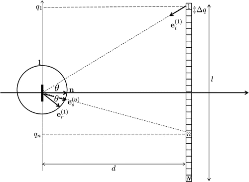
where l is the array length (aperture) as shown in Figure 1. In the analysis below, it is assumed that N is even and that the array elements are evenly spaced (that is the array pitch $\mathrm{\Delta }q$ is constant). The forthcoming analysis is simplified if ${\widehat{q}}_n$ is approximated as a linear function of n. Combining Equations (4(4) $$\begin{array}{c}\hfill {\mathbf{e}}_s^{(n)}=\frac{d}{\sqrt{d^2+y_n^2}}\mathbf{i}+\frac{q_n}{\sqrt{d^2+q_n^2}}\mathbf{j}=\sqrt{1-{\widehat{q}}_n^2}\mathbf{i}+{\widehat{q}}_n\mathbf{j},\end{array}$$(4) )–(6(6) $$\begin{array}{c}\hfill ▵q=\frac{l}{N-1},\end{array}$$(6) ) then(7) $$\begin{array}{c}\hfill {\widehat{q}}_n=\frac{l}{\sqrt{4d^2+l^2{(1-h(n))}^2}}\frac{N+1-2n}{N-1},\end{array}$$(7)

where $h(n)=2(n-1)/(N-1)$. The denominator in the expression for ${\widehat{q}}_n$ in (7(7) $$\begin{array}{c}\hfill {\widehat{q}}_n=\frac{l}{\sqrt{4d^2+l^2{(1-h(n))}^2}}\frac{N+1-2n}{N-1},\end{array}$$(7) ) is manipulated further to give(8) $$\begin{array}{c}\hfill {\widehat{q}}_n=\frac{l}{\sqrt{4d^2+l^2}}\frac{N+1-2n}{N-1}\frac{1}{\sqrt{1-\mathit{\alpha }}},\end{array}$$(8)

where $\mathit{\alpha }=l^2(2h-h^2)/(4d^2+l^2)$. Since $0\le h(n)\le 2$ for $n=1,\dots ,N$ then $0\le 2h-h^2\le 1$, and since $0<l^2/(4d^2+l^2)<1$, then $\mathit{\alpha }$ is small. A Taylor series approximation is applied to Equation (8(8) $$\begin{array}{c}\hfill {\widehat{q}}_n=\frac{l}{\sqrt{4d^2+l^2}}\frac{N+1-2n}{N-1}\frac{1}{\sqrt{1-\mathit{\alpha }}},\end{array}$$(8) ) to approximate ${\widehat{q}}_n$ by ${\widehat{q}}_n={\widehat{y}}_n+\mathcal{O}(\mathit{\alpha })$ where ${\widehat{y}}_n=\mathrm{\Delta }y(N+1-2n)/2$ and $\mathrm{\Delta }y=2l/((N-1)\sqrt{4d^2+l^2})$. Note that in the NDE regime where the quantity $l/(N-1)$ (the array pitch) is of the order ${10}^{-3}$, it holds that $\mathrm{\Delta }y<1$. Additionally, as an approximation to ${\widehat{q}}_n$, ${\widehat{y}}_n\le 1$ (these assumptions are used in the forthcoming analysis). From Equation (4(4) $$\begin{array}{c}\hfill {\mathbf{e}}_s^{(n)}=\frac{d}{\sqrt{d^2+y_n^2}}\mathbf{i}+\frac{q_n}{\sqrt{d^2+q_n^2}}\mathbf{j}=\sqrt{1-{\widehat{q}}_n^2}\mathbf{i}+{\widehat{q}}_n\mathbf{j},\end{array}$$(4) ) the transmitting (on element m) and receiving (on element n) unit vectors are therefore given by(9) $$\begin{array}{c}\hfill {\mathbf{e}}_i^{(m)}=-\sqrt{1-{\widehat{y}}_m^2}\mathbf{i}-{\widehat{y}}_m\mathbf{j},m=1,\dots ,N,\end{array}$$(9)

and(10) $$\begin{array}{c}\hfill {\mathbf{e}}_s^{(n)}=\sqrt{1-{\widehat{y}}_n^2}\mathbf{i}+{\widehat{y}}_n\mathbf{j},n=1,\dots ,N.\end{array}$$(10)

By restricting attention to the case where the flaw is orientated to lie along the $x_2$ axis (i.e. the flaw lies parallel to the ultrasonic array) the specular reflection (denoted by the subscript r) can be written as(11) $$\begin{array}{c}\hfill {\mathbf{e}}_r^{(m)}=\sqrt{1-{\widehat{y}}_m^2}\mathbf{i}-{\widehat{y}}_m\mathbf{j},m=1,\dots ,N,\end{array}$$(11)

mirroring the angle of the incident wave with respect to the crack normal. Finally, since the flaw lies on the $x_2$ axis (that is ${\mathbf{u}}_2=\mathbf{j}$ and n = i), Equation (3(3) $$\begin{array}{cc}\hfill A_n({\mathbf{e}}_i,{\mathbf{e}}_s)& =-\frac{i{a}_2{e}_{sn}(L(({\mathbf{e}}_i-{\mathbf{e}}_r)·\mathbf{n})+2\mathit{\mu }(({\mathbf{e}}_i-{\mathbf{e}}_r)·{\mathbf{e}}_s)({\mathbf{e}}_s·\mathbf{n}))}{2\mathit{\rho }{c}^2|({\mathbf{e}}_i-{\mathbf{e}}_s)·{\mathbf{u}}_2|}\hfill \\ \hfill & \times J_1(\frac{2\mathit{\pi }{a}_2}{\mathit{\lambda }}|({\mathbf{e}}_i-{\mathbf{e}}_s)·{\mathbf{u}}_2|),\hfill \end{array}$$(3) ) becomes(12) $$\begin{array}{c}\hfill A({\widehat{y}}_m,{\widehat{y}}_n)=\frac{\sqrt{1-{\widehat{y}}_m^2}}{\mathit{\rho }{c}^2|{\widehat{y}}_n+{\widehat{y}}_m|}(L+2\mathit{\mu }(1-{\widehat{y}}_n^2))J_1(2\mathit{\pi }{\widehat{a}}_2|{\widehat{y}}_n+{\widehat{y}}_m|)\end{array}$$(12)

where ${\widehat{a}}_2=a_2/\mathit{\lambda }$ is the crack radius to wavelength ratio. In the next section a crack sizing method is developed which relates the maximum eigenvalue of the scattering matrix A to the length of the crack.

4. Crack sizing using the maximum eigenvalue

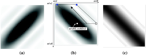
It is clear from empirical observations that there is a relationship between the size of the crack and the form of the scattering matrix [20]. It would therefore be advantageous if an analytical approach could be developed to capture this correlation. From the scattering matrix in Figure 2(a) it can be seen that the dominant values aggregate around the skew diagonal. A diagonal-constant matrix is known as a Toeplitz matrix and there is a considerable body of research concerning these special matrices [23–26]. In an effort to benefit from this body of work, the scattering matrix, A, given by Equation (12(12) $$\begin{array}{c}\hfill A({\widehat{y}}_m,{\widehat{y}}_n)=\frac{\sqrt{1-{\widehat{y}}_m^2}}{\mathit{\rho }{c}^2|{\widehat{y}}_n+{\widehat{y}}_m|}(L+2\mathit{\mu }(1-{\widehat{y}}_n^2))J_1(2\mathit{\pi }{\widehat{a}}_2|{\widehat{y}}_n+{\widehat{y}}_m|)\end{array}$$(12) ), will be approximated by a Toeplitz matrix. First, the matrix A is transformed to $A_T$ via(13) $$\begin{array}{c}\hfill A_T({\widehat{y}}_{m^{\prime }},{\widehat{y}}_n)=A({\widehat{y}}_m,{\widehat{y}}_n)\text{where}{m}^{\prime }=N-m+1\end{array}$$(13)

so that the dominant values accumulate around the main diagonal as shown in Figure 2(b) (this is equivalent to reflecting the matrix entries about a vertical axis centred on the central column). The transformed scattering matrix, $A_T$, will be approximated by a Toeplitz matrix where the row containing the maximum value of $A_T({\widehat{y}}_m,{\widehat{y}}_n)$ is used to create the approximation, ${\overline{A}}_T$. This row is highlighted by the hollow squares in the transformed matrix, $A_T$, in Figure 2(b). This right-most half row (N / 2 entries) is then used as the generator of a Toeplitz matrix. The resulting matrix is shown in Figure 2(c). To begin we observe that in Equation (12(12) $$\begin{array}{c}\hfill A({\widehat{y}}_m,{\widehat{y}}_n)=\frac{\sqrt{1-{\widehat{y}}_m^2}}{\mathit{\rho }{c}^2|{\widehat{y}}_n+{\widehat{y}}_m|}(L+2\mathit{\mu }(1-{\widehat{y}}_n^2))J_1(2\mathit{\pi }{\widehat{a}}_2|{\widehat{y}}_n+{\widehat{y}}_m|)\end{array}$$(12) ) the term(14) $$\begin{array}{c}\hfill \frac{J_1\left(2\mathit{\pi }{\widehat{a}}_2({\widehat{y}}_n+{\widehat{y}}_m)\right)}{{\widehat{y}}_n+{\widehat{y}}_m}\end{array}$$(14)

obtains its maximum when ${\widehat{y}}_n+{\widehat{y}}_m=0$. The prefactor to the Bessel function in Equation (12(12) $$\begin{array}{c}\hfill A({\widehat{y}}_m,{\widehat{y}}_n)=\frac{\sqrt{1-{\widehat{y}}_m^2}}{\mathit{\rho }{c}^2|{\widehat{y}}_n+{\widehat{y}}_m|}(L+2\mathit{\mu }(1-{\widehat{y}}_n^2))J_1(2\mathit{\pi }{\widehat{a}}_2|{\widehat{y}}_n+{\widehat{y}}_m|)\end{array}$$(12) ) is given by(15) $$\begin{array}{c}\hfill \sqrt{1-{\widehat{y}}_m^2}(L+2\mathit{\mu }(1-{\widehat{y}}_{n^{\prime }}^2)),\end{array}$$(15)

and, since $0\le {\widehat{y}}_m^2,{\widehat{y}}_n^2\le 1$ (see Section 3), is also maximized when ${\widehat{y}}_m={\widehat{y}}_n=0$. As the array is centred on the $x_1$-axis, this means that ${\widehat{y}}_m={\widehat{y}}_n=0$ corresponds to the centre of the array. If N is odd then the central element is given by $n=m=(N+1)/2$ and if N is even then the smallest value is ${\widehat{y}}_m={\widehat{y}}_n=-▵y/2$ which occurs at $n=m=N/2+1$. In what follows the focus will be on the case where N is even (the analysis is virtually identical for the case where N is odd) and so we will take this row of A (and hence $A_T$) to form our Toeplitz approximation. Substituting ${\widehat{y}}_m=-▵y/2$ into Equation (12(12) $$\begin{array}{c}\hfill A({\widehat{y}}_m,{\widehat{y}}_n)=\frac{\sqrt{1-{\widehat{y}}_m^2}}{\mathit{\rho }{c}^2|{\widehat{y}}_n+{\widehat{y}}_m|}(L+2\mathit{\mu }(1-{\widehat{y}}_n^2))J_1(2\mathit{\pi }{\widehat{a}}_2|{\widehat{y}}_n+{\widehat{y}}_m|)\end{array}$$(12) ) gives the first N / 2 entries in the first row of the Toeplitz matrix ${\overline{A}}_T$ as(16) $$\begin{array}{c}\hfill {\overline{A}}_T({\widehat{y}}_p)=\frac{2\sqrt{1-▵y^2/4}(L+2\mathit{\mu }(1-{\widehat{y}}_p^2))}{\mathit{\rho }{c}^2(2{\widehat{y}}_p-▵y)}{J}_1(2\mathit{\pi }{\widehat{a}}_2\left({\widehat{y}}_p-\frac{▵y}{2}\right)),\end{array}$$(16)

where $p=N/2+1,\dots ,N$; this row is highlighted in the scattering matrix shown in Figure 2(b). The remaining terms in the first row of ${\overline{A}}_T$ are set equal to zero (that is ${\overline{A}}_T({\widehat{y}}_j)=0,j=N/2+1,\dots ,N$, see Figure 2(c)). Note that the absolute value present in Equation (12(12) $$\begin{array}{c}\hfill A({\widehat{y}}_m,{\widehat{y}}_n)=\frac{\sqrt{1-{\widehat{y}}_m^2}}{\mathit{\rho }{c}^2|{\widehat{y}}_n+{\widehat{y}}_m|}(L+2\mathit{\mu }(1-{\widehat{y}}_n^2))J_1(2\mathit{\pi }{\widehat{a}}_2|{\widehat{y}}_n+{\widehat{y}}_m|)\end{array}$$(12) ) has been removed since ${\widehat{y}}_p-▵y/2<0$ and $-3.8317<2\mathit{\pi }{\widehat{a}}_2({\widehat{y}}_p-▵y/2)<0$ in our regime of interest and so it follows that $J_1(2\mathit{\pi }{\widehat{a}}_2({\widehat{y}}_p-▵y/2))<0$.

Figure 2. The original scattering matrix, A (Equation (12(12) $$\begin{array}{c}\hfill A({\widehat{y}}_m,{\widehat{y}}_n)=\frac{\sqrt{1-{\widehat{y}}_m^2}}{\mathit{\rho }{c}^2|{\widehat{y}}_n+{\widehat{y}}_m|}(L+2\mathit{\mu }(1-{\widehat{y}}_n^2))J_1(2\mathit{\pi }{\widehat{a}}_2|{\widehat{y}}_n+{\widehat{y}}_m|)\end{array}$$(12) ), is shown in (a). The transformed matrix $A_T$ (Equation (13(13) $$\begin{array}{c}\hfill A_T({\widehat{y}}_{m^{\prime }},{\widehat{y}}_n)=A({\widehat{y}}_m,{\widehat{y}}_n)\text{where}{m}^{\prime }=N-m+1\end{array}$$(13) )) is shown in (b) where the hollow squares highlight the section of the row which is used to construct the Toeplitz approximation. This is the row where the maximum occurs at $n=m=N/2+1$. The black lines highlight the rows which are shown to be approximately equal to the portion of the row where the maximum occurs. Matrix (c) shows the Toeplitz matrix, ${\overline{A}}_T$, constructed using the row where the maximum occurs.

4.1. An approximation for the maximum eigenvalue of the Toeplitz form of the scattering matrix

In the forthcoming section an approximation which relates the crack radius to wavelength ratio, ${\widehat{a}}_2=a_2/\mathit{\lambda }$, to the maximum eigenvalue ${\mathit{\sigma }}_{max}$ of the Toeplitz matrix used to approximate to the scattering matrix is derived. This maximum eigenvalue is approximated using an upper bound, ${\mathit{\sigma }}_B$, which is given by [27](17) $$\begin{array}{c}\hfill {\mathit{\sigma }}_B={({\overline{A}}_T)}_1·\mathbf{w}\end{array}$$(17)

where ${({\overline{A}}_T)}_1$ denotes the first row of the matrix ${({\overline{A}}_T)}_1=({({\overline{A}}_T)}_{1,1},|{({\overline{A}}_T)}_{1,2}|,\dots ,|{({\overline{A}}_T)}_{1,N}|)$, $\mathbf{w}=(1,w_2,\dots ,w_N)$ with(18) $$\begin{array}{c}\hfill w_k=2cos(\frac{\mathit{\pi }}{\lfloor \frac{N-1}{k-1}\rfloor +2}),k=2,\dots ,N,\end{array}$$(18)

and $\lfloor .\rfloor$ denotes the floor function. The first row of the Toeplitz matrix, ${\overline{A}}_T({\widehat{y}}_p)$, is given by Equation (16(16) $$\begin{array}{c}\hfill {\overline{A}}_T({\widehat{y}}_p)=\frac{2\sqrt{1-▵y^2/4}(L+2\mathit{\mu }(1-{\widehat{y}}_p^2))}{\mathit{\rho }{c}^2(2{\widehat{y}}_p-▵y)}{J}_1(2\mathit{\pi }{\widehat{a}}_2\left({\widehat{y}}_p-\frac{▵y}{2}\right)),\end{array}$$(16) ) and when substituted into Equation (17(17) $$\begin{array}{c}\hfill {\mathit{\sigma }}_B={({\overline{A}}_T)}_1·\mathbf{w}\end{array}$$(17) ) the maximum eigenvalue approximation can be written(19) $$\begin{array}{cc}\hfill {\mathit{\sigma }}_B& ={\overline{A}}_T({\widehat{y}}_{N/2+1})+\sum _{t=N/2+2}^N|A_T({\widehat{y}}_t)|w_t\hfill \\ \hfill & ={\overline{A}}_T({\widehat{y}}_{N/2+1})+\sum _{t=N/2+2}^N{F}_t({\widehat{a}}_2)\frac{J_1\left(2\mathit{\pi }{\widehat{a}}_2\left({\widehat{y}}_t-▵y/2\right)\right)}{2\mathit{\pi }{\widehat{a}}_2\left({\widehat{y}}_t-▵y/2\right)}{w}_t,\hfill \end{array}$$(19)

where(20) $$\begin{array}{c}\hfill w_t=2cos(\frac{\mathit{\pi }}{\lfloor \frac{2(N-1)}{2t-2-N}\rfloor +2}),\end{array}$$(20)

with $k=t-N/2$, and the prefactor is given by(21) $$\begin{array}{c}\hfill F_t({\widehat{a}}_2)=\frac{2\mathit{\pi }{\widehat{a}}_2\sqrt{1-{(▵y)}^2/4}}{\mathit{\rho }{c}^2}(L+2\mathit{\mu }(1-{\widehat{y}}_t^2)).\end{array}$$(21)

In order to view the explicit dependency of ${\mathit{\sigma }}_B$ on ${\widehat{a}}_2$ it is necessary to make approximations to the expression within the summation in Equation (19(19) $$\begin{array}{cc}\hfill {\mathit{\sigma }}_B& ={\overline{A}}_T({\widehat{y}}_{N/2+1})+\sum _{t=N/2+2}^N|A_T({\widehat{y}}_t)|w_t\hfill \\ \hfill & ={\overline{A}}_T({\widehat{y}}_{N/2+1})+\sum _{t=N/2+2}^N{F}_t({\widehat{a}}_2)\frac{J_1\left(2\mathit{\pi }{\widehat{a}}_2\left({\widehat{y}}_t-▵y/2\right)\right)}{2\mathit{\pi }{\widehat{a}}_2\left({\widehat{y}}_t-▵y/2\right)}{w}_t,\hfill \end{array}$$(19) ). The Bessel function within Equation (19(19) $$\begin{array}{cc}\hfill {\mathit{\sigma }}_B& ={\overline{A}}_T({\widehat{y}}_{N/2+1})+\sum _{t=N/2+2}^N|A_T({\widehat{y}}_t)|w_t\hfill \\ \hfill & ={\overline{A}}_T({\widehat{y}}_{N/2+1})+\sum _{t=N/2+2}^N{F}_t({\widehat{a}}_2)\frac{J_1\left(2\mathit{\pi }{\widehat{a}}_2\left({\widehat{y}}_t-▵y/2\right)\right)}{2\mathit{\pi }{\widehat{a}}_2\left({\widehat{y}}_t-▵y/2\right)}{w}_t,\hfill \end{array}$$(19) ) is approximated by$$\begin{array}{c}\hfill \frac{J_1\left(2\mathit{\pi }{\widehat{a}}_2\left({\widehat{y}}_t-▵y/2\right)\right)}{2\mathit{\pi }{\widehat{a}}_2\left({\widehat{y}}_t-▵y/2\right)}=\left\{\begin{array}{cc}{f}_t^{(1)}({\widehat{a}}_2)\hfill & \text{if}N/2+2\le t\le t^{\ast }\hfill \\ f_t^{(2)}({\widehat{a}}_2)\hfill & \text{if}{t}^{\ast }+1\le t\le N\hfill \end{array}\right.\end{array}$$

where the approximation for small arguments [28] is used to give(22) $$\begin{array}{c}\hfill f_t^{(1)}(t,{\widehat{a}}_2)\approx \frac{1}{2}\left(1-\frac{1}{4}{\left(\mathit{\pi }{\widehat{a}}_2\left({\widehat{y}}_t-\frac{▵y}{2}\right)\right)}^2\right),\end{array}$$(22)

and for large arguments [28](23) $$\begin{array}{cc}\hfill f_t^{(2)}(t,{\widehat{a}}_2)& \approx \frac{1}{2{\mathit{\pi }}^2}{\left({\widehat{a}}_2\left({\widehat{y}}_t-\frac{▵y}{2}\right)\right)}^{-\frac{3}{2}}cos(2\mathit{\pi }{\widehat{a}}_2\left({\widehat{y}}_t-\frac{▵y}{2}\right)-\frac{3\mathit{\pi }}{4}).\hfill \end{array}$$(23)

The index $t^{\ast }$ determines when the argument of the Bessel function converts from small values to large values (an expression for $t^{\ast }$ can be determined as a function of the system parameters and ${\widehat{a}}_2$ [29] ). Evaluating Equation (16(16) $$\begin{array}{c}\hfill {\overline{A}}_T({\widehat{y}}_p)=\frac{2\sqrt{1-▵y^2/4}(L+2\mathit{\mu }(1-{\widehat{y}}_p^2))}{\mathit{\rho }{c}^2(2{\widehat{y}}_p-▵y)}{J}_1(2\mathit{\pi }{\widehat{a}}_2\left({\widehat{y}}_p-\frac{▵y}{2}\right)),\end{array}$$(16) ) at $p=N/2+1$ gives(24) $$\begin{array}{c}\hfill {\overline{A}}_T\left(-\frac{▵y}{2}\right)=F_{N/2+1}({\widehat{a}}_2)=\frac{2{\widehat{a}}_2\mathit{\pi }\sqrt{1-{(▵y)}^2/4}\left(L+2\mathit{\mu }\left(1-{(▵y)}^2/4\right)\right)}{\mathit{\rho }{c}^2},\end{array}$$(24)

where $0<▵y<1$. The approximation to Equation (19(19) $$\begin{array}{cc}\hfill {\mathit{\sigma }}_B& ={\overline{A}}_T({\widehat{y}}_{N/2+1})+\sum _{t=N/2+2}^N|A_T({\widehat{y}}_t)|w_t\hfill \\ \hfill & ={\overline{A}}_T({\widehat{y}}_{N/2+1})+\sum _{t=N/2+2}^N{F}_t({\widehat{a}}_2)\frac{J_1\left(2\mathit{\pi }{\widehat{a}}_2\left({\widehat{y}}_t-▵y/2\right)\right)}{2\mathit{\pi }{\widehat{a}}_2\left({\widehat{y}}_t-▵y/2\right)}{w}_t,\hfill \end{array}$$(19) ) is split into two summations and is therefore given by(25) $$\begin{array}{cc}\hfill {\mathit{\sigma }}_B& \approx F_{N/2+1}({\widehat{a}}_2)+\sum _{t=N/2+1}^{t^{\ast }}{F}_t({\widehat{a}}_2)f_t^{(1)}({\widehat{a}}_2)w_t+\sum _{t=t^{\ast }+1}^N{F}_t({\widehat{a}}_2)f_t^{(2)}({\widehat{a}}_2)w_t.\hfill \end{array}$$(25)

Further approximations are applied to Equation (23(23) $$\begin{array}{cc}\hfill f_t^{(2)}(t,{\widehat{a}}_2)& \approx \frac{1}{2{\mathit{\pi }}^2}{\left({\widehat{a}}_2\left({\widehat{y}}_t-\frac{▵y}{2}\right)\right)}^{-\frac{3}{2}}cos(2\mathit{\pi }{\widehat{a}}_2\left({\widehat{y}}_t-\frac{▵y}{2}\right)-\frac{3\mathit{\pi }}{4}).\hfill \end{array}$$(23) ) to allow ${\mathit{\sigma }}_B$ to be expressed in terms of a polynomial in t. This will be useful later where the aim is to extract the parameter ${\widehat{a}}_2$ in order to obtain an explicit expression which relates ${\mathit{\sigma }}_B$ to ${\widehat{a}}_2$. Let $f_t^{(2)}({\widehat{a}}_2)=s_t^{(1)}({\widehat{a}}_2)s_t^{(2)}({\widehat{a}}_2)$ where(26) $$\begin{array}{cc}\hfill s_t^{(1)}({\widehat{a}}_2)& =\frac{1}{{\mathit{\pi }}^2}(\frac{2}{{\widehat{a}}_2▵y(N-2t)}{)}^{\frac{3}{2}}\hfill \end{array}$$(26)

and(27) $$\begin{array}{cc}\hfill s_t^{(2)}({\widehat{a}}_2)& =cos(\mathit{\pi }{\widehat{a}}_2▵y(N-2t)-\frac{3\mathit{\pi }}{4}).\hfill \end{array}$$(27)

By taking Taylor series expansions of these expressions around the point $m=(t^{\ast }+N)/2$ (the midpoint between $t^{\ast }$ and N), we yield the approximations(28) $$\begin{array}{cc}\hfill {\overline{s}}_t^{(1)}({\widehat{a}}_2,m)& =\frac{1}{2{\mathit{\pi }}^2}{\left(\frac{1}{{\widehat{a}}_2▵y(N-2m)}\right)}^{3/2}\left(1+\frac{3}{N-2m}(t-m)\right)\hfill \end{array}$$(28)

and(29) $$\begin{array}{cc}\hfill {\overline{s}}_t^{(2)}({\widehat{a}}_2,m)& =cos(\mathit{\pi }{\widehat{a}}_2▵y(N-2m)-\frac{3\mathit{\pi }}{4})(1-2({\widehat{a}}_2\mathit{\pi }▵y(t-m){)}^2)\hfill \\ \hfill & +sin(\mathit{\pi }{\widehat{a}}_2▵y(N-2m)-\frac{3\mathit{\pi }}{4})(-2{\widehat{a}}_2\mathit{\pi }▵y(t-m)+\frac{4}{3}({\widehat{a}}_2\mathit{\pi }▵y(t-m){)}^3).\hfill \end{array}$$(29)

We now approximate $f_t^{(2)}$ by(30) $$\begin{array}{cc}\hfill {\overline{f}}_t^{(2)}({\widehat{a}}_2,m)& ={\overline{s}}_t^{(1)}({\widehat{a}}_2,m){\overline{s}}_t^{(2)}({\widehat{a}}_2,m).\hfill \end{array}$$(30)

Substituting Equations (28(28) $$\begin{array}{cc}\hfill {\overline{s}}_t^{(1)}({\widehat{a}}_2,m)& =\frac{1}{2{\mathit{\pi }}^2}{\left(\frac{1}{{\widehat{a}}_2▵y(N-2m)}\right)}^{3/2}\left(1+\frac{3}{N-2m}(t-m)\right)\hfill \end{array}$$(28) ) and (29(29) $$\begin{array}{cc}\hfill {\overline{s}}_t^{(2)}({\widehat{a}}_2,m)& =cos(\mathit{\pi }{\widehat{a}}_2▵y(N-2m)-\frac{3\mathit{\pi }}{4})(1-2({\widehat{a}}_2\mathit{\pi }▵y(t-m){)}^2)\hfill \\ \hfill & +sin(\mathit{\pi }{\widehat{a}}_2▵y(N-2m)-\frac{3\mathit{\pi }}{4})(-2{\widehat{a}}_2\mathit{\pi }▵y(t-m)+\frac{4}{3}({\widehat{a}}_2\mathit{\pi }▵y(t-m){)}^3).\hfill \end{array}$$(29) ) into Equation (25(25) $$\begin{array}{cc}\hfill {\mathit{\sigma }}_B& \approx F_{N/2+1}({\widehat{a}}_2)+\sum _{t=N/2+1}^{t^{\ast }}{F}_t({\widehat{a}}_2)f_t^{(1)}({\widehat{a}}_2)w_t+\sum _{t=t^{\ast }+1}^N{F}_t({\widehat{a}}_2)f_t^{(2)}({\widehat{a}}_2)w_t.\hfill \end{array}$$(25) ) gives an approximate expression for ${\mathit{\sigma }}_B$:(31) $$\begin{array}{cc}\hfill {\mathit{\sigma }}_B& \approx F_{N/2+1}({\widehat{a}}_2)+\sum _{t=p+1}^{t^{\ast }}{F}_t({\widehat{a}}_2)f_t^{(1)}{w}_t\hfill \\ \hfill & +\sum _{t=t^{\ast }}^N{F}_t({\widehat{a}}_2){\overline{s}}_t^{(1)}({\widehat{a}}_2,m){\overline{s}}_t^{(2)}({\widehat{a}}_2,m)w_t.\hfill \end{array}$$(31)

Finally, $w_t$ given by Equation (20(20) $$\begin{array}{c}\hfill w_t=2cos(\frac{\mathit{\pi }}{\lfloor \frac{2(N-1)}{2t-2-N}\rfloor +2}),\end{array}$$(20) ) is approximated by a linear function. First the floor function within the cosine in Equation (18(18) $$\begin{array}{c}\hfill w_k=2cos(\frac{\mathit{\pi }}{\lfloor \frac{N-1}{k-1}\rfloor +2}),k=2,\dots ,N,\end{array}$$(18) ) is dropped (a justification is given in [29]) to give(32) $$\begin{array}{c}\hfill w_t=2cos\left(\frac{\mathit{\pi }(2t-2-N)}{2(2t-3)}\right).\end{array}$$(32)

The function is then approximated by a Taylor series about 3N / 4 (the midpoint in the range $t=N/2+1$ to $t=N$) to give(33) $$\begin{array}{cc}\hfill {\overline{w}}_t(N)& =2cos\left(\frac{\mathit{\pi }(N-4)}{6(N-2)}\right)-\frac{8\mathit{\pi }(N-1)\left(t-3N/4\right)}{9{(N-2)}^2}sin\left(\frac{\mathit{\pi }(N-4)}{6(N-2)}\right).\hfill \end{array}$$(33)

This is substituted into Equation (31(31) $$\begin{array}{cc}\hfill {\mathit{\sigma }}_B& \approx F_{N/2+1}({\widehat{a}}_2)+\sum _{t=p+1}^{t^{\ast }}{F}_t({\widehat{a}}_2)f_t^{(1)}{w}_t\hfill \\ \hfill & +\sum _{t=t^{\ast }}^N{F}_t({\widehat{a}}_2){\overline{s}}_t^{(1)}({\widehat{a}}_2,m){\overline{s}}_t^{(2)}({\widehat{a}}_2,m)w_t.\hfill \end{array}$$(31) ) to obtain(34) $$\begin{array}{cc}\hfill {\mathit{\sigma }}_B& =F_{N/2+1}({\widehat{a}}_2)\hfill \\ \hfill & +\sum _{t=N/2+2}^{t^{\ast }}{F}_t({\widehat{a}}_2)f_t^{(1)}{\overline{w}}_t(N)\hfill \\ \hfill & +\sum _{t=t^{\ast }}^N{F}_t({\widehat{a}}_2){\overline{s}}_t^{(1)}({\widehat{a}}_2,m){\overline{s}}_t^{(2)}({\widehat{a}}_2,m){\overline{w}}_t(N).\hfill \end{array}$$(34)

The first summation in Equation (34(34) $$\begin{array}{cc}\hfill {\mathit{\sigma }}_B& =F_{N/2+1}({\widehat{a}}_2)\hfill \\ \hfill & +\sum _{t=N/2+2}^{t^{\ast }}{F}_t({\widehat{a}}_2)f_t^{(1)}{\overline{w}}_t(N)\hfill \\ \hfill & +\sum _{t=t^{\ast }}^N{F}_t({\widehat{a}}_2){\overline{s}}_t^{(1)}({\widehat{a}}_2,m){\overline{s}}_t^{(2)}({\widehat{a}}_2,m){\overline{w}}_t(N).\hfill \end{array}$$(34) ) involves the product of three terms. Since $y_t$ is a linear function of the index t then from Equation (21(21) $$\begin{array}{c}\hfill F_t({\widehat{a}}_2)=\frac{2\mathit{\pi }{\widehat{a}}_2\sqrt{1-{(▵y)}^2/4}}{\mathit{\rho }{c}^2}(L+2\mathit{\mu }(1-{\widehat{y}}_t^2)).\end{array}$$(21) ) $F_t({\widehat{a}}_2)$ is a quadratic function in t, from Equation (22(22) $$\begin{array}{c}\hfill f_t^{(1)}(t,{\widehat{a}}_2)\approx \frac{1}{2}\left(1-\frac{1}{4}{\left(\mathit{\pi }{\widehat{a}}_2\left({\widehat{y}}_t-\frac{▵y}{2}\right)\right)}^2\right),\end{array}$$(22) ) $f_t^{(1)}$ is a quadratic function in t, and from Equation (33(33) $$\begin{array}{cc}\hfill {\overline{w}}_t(N)& =2cos\left(\frac{\mathit{\pi }(N-4)}{6(N-2)}\right)-\frac{8\mathit{\pi }(N-1)\left(t-3N/4\right)}{9{(N-2)}^2}sin\left(\frac{\mathit{\pi }(N-4)}{6(N-2)}\right).\hfill \end{array}$$(33) ) ${\overline{w}}_t(N)$ is a linear function of t. Therefore, this first summation is a fifth order polynomial in t. Similarly, the second summation in Equation (34(34) $$\begin{array}{cc}\hfill {\mathit{\sigma }}_B& =F_{N/2+1}({\widehat{a}}_2)\hfill \\ \hfill & +\sum _{t=N/2+2}^{t^{\ast }}{F}_t({\widehat{a}}_2)f_t^{(1)}{\overline{w}}_t(N)\hfill \\ \hfill & +\sum _{t=t^{\ast }}^N{F}_t({\widehat{a}}_2){\overline{s}}_t^{(1)}({\widehat{a}}_2,m){\overline{s}}_t^{(2)}({\widehat{a}}_2,m){\overline{w}}_t(N).\hfill \end{array}$$(34) ) involves the product of four terms. From Equation (28(28) $$\begin{array}{cc}\hfill {\overline{s}}_t^{(1)}({\widehat{a}}_2,m)& =\frac{1}{2{\mathit{\pi }}^2}{\left(\frac{1}{{\widehat{a}}_2▵y(N-2m)}\right)}^{3/2}\left(1+\frac{3}{N-2m}(t-m)\right)\hfill \end{array}$$(28) ) ${\overline{s}}_t^{(1)}$ is linear in t, and from Equation (29(29) $$\begin{array}{cc}\hfill {\overline{s}}_t^{(2)}({\widehat{a}}_2,m)& =cos(\mathit{\pi }{\widehat{a}}_2▵y(N-2m)-\frac{3\mathit{\pi }}{4})(1-2({\widehat{a}}_2\mathit{\pi }▵y(t-m){)}^2)\hfill \\ \hfill & +sin(\mathit{\pi }{\widehat{a}}_2▵y(N-2m)-\frac{3\mathit{\pi }}{4})(-2{\widehat{a}}_2\mathit{\pi }▵y(t-m)+\frac{4}{3}({\widehat{a}}_2\mathit{\pi }▵y(t-m){)}^3).\hfill \end{array}$$(29) ) ${\overline{s}}_t^{(2)}$ is cubic in t, and so this second summation is a seventh order polynomial in t. Hence this allows ${\mathit{\sigma }}_B$ to be expressed in the following form(35) $$\begin{array}{c}\hfill {\mathit{\sigma }}_B=\widehat{A}{\widehat{a}}_2+\sum _{l=1}^6{S}_l^{(1)}({\widehat{a}}_2)b_l({\widehat{a}}_2)+\sum _{l=1}^8{S}_l^{(2)}({\widehat{a}}_2)d_l({\widehat{a}}_2),\end{array}$$(35)

where(36) $$\begin{array}{cc}\hfill \widehat{A}& =\frac{\mathit{\pi }\sqrt{(1-▵y^2/4)}(L+2\mathit{\mu }\left(1-▵y^2/4\right))}{\mathit{\rho }{c}^2},\hfill \end{array}$$(36) (37) $$\begin{array}{cc}\hfill S_l^{(1)}({\widehat{a}}_2)& =\sum _{t=N/2+2}^{t^{\ast }}{t}^{l-1},S_l^{(2)}({\widehat{a}}_2)=\sum _{t=t^{\ast }+1}^N{t}^{l-1},\hfill \end{array}$$(37)

and $b_l$ and $d_l$ are functions of ${\widehat{a}}_2$. Since $t^{\ast }$ is a function of ${\widehat{a}}_2$ then to derive an equation where the dependency on ${\widehat{a}}_2$ is explicit, it is necessary to rewrite these summations so that $t^{\ast }$ does not appear as a limit. Using a closed form expression for the sum to n terms of $t^p$ [30] then(38) $$\begin{array}{cc}\hfill S_l^{(1)}({\widehat{a}}_2)& =\frac{{(t^{\ast }+1)}^l}{l}+\sum _{k=1}^l\frac{B_k}{l-k}\left(\begin{array}{c}l-1\\ k\end{array}\right){(t^{\ast }+1)}^{l-k}-\frac{{(N/2+2)}^l}{l}\hfill \\ \hfill & -\sum _{k=1}^l\frac{B_k}{l-k}\left(\begin{array}{c}l-1\\ k\end{array}\right){\left(\frac{N}{2}+2\right)}^{l-k}\hfill \end{array}$$(38)

and(39) $$\begin{array}{cc}\hfill S_l^{(2)}({\widehat{a}}_2)& =\frac{{(N+1)}^l}{l}+\sum _{k=1}^l\frac{B_k}{l-k}\left(\begin{array}{c}l-1\\ k\end{array}\right){(N+1)}^{l-k}-\frac{{(t^{\ast }+1)}^l}{l}\hfill \\ & -\sum _{k=1}^l\frac{B_k}{l-k}\left(\begin{array}{c}l-1\\ k\end{array}\right){\left(t^{\ast }+1\right)}^{l-k}\hfill \end{array}$$(39)

where $B_k$ is the kth Bernoulli number. The coefficients $b_l$ are expressed in terms of a polynomial function in ${\widehat{a}}_2$ as $b_l({\widehat{a}}_2)=b_l^{(1)}{\widehat{a}}_2+b_l^{(2)}{\widehat{a}}_2^3$ where $b_l^{(1)}$ and $b_l^{(2)}$ are functions of the number of elements in the array, N, $▵y$, Lamé coefficients L and $\mathit{\mu }$, wave speed c and material density $\mathit{\rho }$. The dependency on ${\widehat{a}}_2$ is extracted from the first summation in Equation (35(35) $$\begin{array}{c}\hfill {\mathit{\sigma }}_B=\widehat{A}{\widehat{a}}_2+\sum _{l=1}^6{S}_l^{(1)}({\widehat{a}}_2)b_l({\widehat{a}}_2)+\sum _{l=1}^8{S}_l^{(2)}({\widehat{a}}_2)d_l({\widehat{a}}_2),\end{array}$$(35) ) to give(40) $$\begin{array}{cc}\hfill \sum _{l=1}^6{S}_l^{(1)}({\widehat{a}}_2)b_l({\widehat{a}}_2)& =\sum _{l=1}^6{S}_l^{(1)}({\widehat{a}}_2)(b_l^{(1)}{\widehat{a}}_2+b_l^{(2)}{\widehat{a}}_2^3)\hfill \\ \hfill & ={\widehat{a}}_2{\widehat{S}}_1({\widehat{a}}_2)+{\widehat{a}}_2^3{\widehat{S}}_2({\widehat{a}}_2)\hfill \end{array}$$(40)

where(41) $$\begin{array}{c}\hfill {\widehat{S}}_1({\widehat{a}}_2)=\sum _{l=1}^6{S}_l^{(1)}({\widehat{a}}_2)b_l^{(1)}\text{and}{\widehat{S}}_2({\widehat{a}}_2)=\sum _{l=1}^6{S}_l^{(1)}({\widehat{a}}_2)b_l^{(2)}.\end{array}$$(41)

The coefficients $d_l$ are extracted from the second summation in Equation (35(35) $$\begin{array}{c}\hfill {\mathit{\sigma }}_B=\widehat{A}{\widehat{a}}_2+\sum _{l=1}^6{S}_l^{(1)}({\widehat{a}}_2)b_l({\widehat{a}}_2)+\sum _{l=1}^8{S}_l^{(2)}({\widehat{a}}_2)d_l({\widehat{a}}_2),\end{array}$$(35) ) and are of the form(42) $$\begin{array}{cc}\hfill d_l({\widehat{a}}_2)& =B({\widehat{a}}_2)(((d_l^{(0)}+d_l^{(1)}{\widehat{a}}_2+d_l^{(2)}{\widehat{a}}_2^2+d_l^{(3)}{\widehat{a}}_2^3+d_l^{(4)}{\widehat{a}}_2^4)cos(p({\widehat{a}}_2))\hfill \\ \hfill & +(d_l^{(5)}+d_l^{(6)}{\widehat{a}}_2+d_l^{(7)}{\widehat{a}}_2^2+d_l^{(8)}{\widehat{a}}_2^3+d_l^{(9)}{\widehat{a}}_2^4)sin(p({\widehat{a}}_2))),\hfill \end{array}$$(42)

where(43) $$\begin{array}{c}\hfill B({\widehat{a}}_2)={\left(\frac{1}{\mathit{\pi }{\widehat{a}}_2▵y(2N-2t^{\ast }-3)}\right)}^{5/2},\end{array}$$(43)

and(44) $$\begin{array}{c}\hfill p({\widehat{a}}_2)=\frac{\mathit{\pi }}{4}+{\widehat{a}}_2\mathit{\pi }▵y{t}^{\ast }.\end{array}$$(44)

The second summation in the expression for ${\mathit{\sigma }}_B$, Equation (35(35) $$\begin{array}{c}\hfill {\mathit{\sigma }}_B=\widehat{A}{\widehat{a}}_2+\sum _{l=1}^6{S}_l^{(1)}({\widehat{a}}_2)b_l({\widehat{a}}_2)+\sum _{l=1}^8{S}_l^{(2)}({\widehat{a}}_2)d_l({\widehat{a}}_2),\end{array}$$(35) ), can now be expressed in the form(45) $$\begin{array}{cc}\hfill \sum _{l=1}^8{S}_l^{(2)}({\widehat{a}}_2)d_l({\widehat{a}}_2)& =B\sum _{l=1}^8{S}_l^{(2)}({\widehat{a}}_2)((d_l^{(0)}+{\widehat{a}}_2{d}_l^{(1)}+{\widehat{a}}_2^2{d}_l^{(2)}+{\widehat{a}}_2^3{d}_l^{(3)}+{\widehat{a}}_2^4{d}_l^{(4)})cos(p({\widehat{a}}_2))\hfill \\ \hfill & +(d_l^{(5)}+{\widehat{a}}_2{d}_l^{(6)}+{\widehat{a}}_2^2{d}_l^{(7)}+{\widehat{a}}_2^3{d}_l^{(8)}+{\widehat{a}}_2^4{d}_l^{(9)})sin(p({\widehat{a}}_2)))\hfill \\ \hfill & ={\widehat{S}}_3({\widehat{a}}_2)cos(p({\widehat{a}}_2))+{\widehat{S}}_4({\widehat{a}}_2)sin(p({\widehat{a}}_2)),\hfill \end{array}$$(45)

with(46) $$\begin{array}{cc}\hfill {\widehat{S}}_3({\widehat{a}}_2)& =B({\widehat{a}}_2)(D_0+D_1{\widehat{a}}_2+D_2{\widehat{a}}_2^2+D_3{\widehat{a}}_2^3+D_4{\widehat{a}}_2^4)\hfill \\ \hfill & =B({\widehat{a}}_2)\sum _{k=0}^4{D}_k({\widehat{a}}_2){\widehat{a}}_2^k\hfill \end{array}$$(46)

and(47) $$\begin{array}{cc}\hfill {\widehat{S}}_4({\widehat{a}}_2)& =B({\widehat{a}}_2)(D_5+D_6{\widehat{a}}_2+D_7{\widehat{a}}_2^2+D_8{\widehat{a}}_2^3+D_9{\widehat{a}}_2^4)\hfill \\ \hfill & =B({\widehat{a}}_2)\sum _{k=5}^9{D}_k({\widehat{a}}_2){\widehat{a}}_2^{k-5},\hfill \end{array}$$(47)

where(48) $$\begin{array}{c}\hfill D_j({\widehat{a}}_2)=\sum _{l=1}^8{S}_l^{(2)}({\widehat{a}}_2)d_l^{(j)}.\end{array}$$(48)

The terms $d_l^{(i)}$ where $i=1,\dots ,10$ and $l=1,\dots ,8$ are independent of ${\widehat{a}}_2$ and again are functions of the system parameters. The expression in Equation (45(45) $$\begin{array}{cc}\hfill \sum _{l=1}^8{S}_l^{(2)}({\widehat{a}}_2)d_l({\widehat{a}}_2)& =B\sum _{l=1}^8{S}_l^{(2)}({\widehat{a}}_2)((d_l^{(0)}+{\widehat{a}}_2{d}_l^{(1)}+{\widehat{a}}_2^2{d}_l^{(2)}+{\widehat{a}}_2^3{d}_l^{(3)}+{\widehat{a}}_2^4{d}_l^{(4)})cos(p({\widehat{a}}_2))\hfill \\ \hfill & +(d_l^{(5)}+{\widehat{a}}_2{d}_l^{(6)}+{\widehat{a}}_2^2{d}_l^{(7)}+{\widehat{a}}_2^3{d}_l^{(8)}+{\widehat{a}}_2^4{d}_l^{(9)})sin(p({\widehat{a}}_2)))\hfill \\ \hfill & ={\widehat{S}}_3({\widehat{a}}_2)cos(p({\widehat{a}}_2))+{\widehat{S}}_4({\widehat{a}}_2)sin(p({\widehat{a}}_2)),\hfill \end{array}$$(45) ) can then be expressed in the form(49) $$\begin{array}{c}\hfill \sum _{l=1}^8{S}_l^{(2)}({\widehat{a}}_2)d_l({\widehat{a}}_2)=Q({\widehat{a}}_2)cos(p({\widehat{a}}_2)-\mathit{\varphi }({\widehat{a}}_2)),\end{array}$$(49)

where $\mathit{\varphi }({\widehat{a}}_2)={tan}^{-1}\left({\widehat{S}}_4({\widehat{a}}_2)/{\widehat{S}}_3({\widehat{a}}_2)\right)$ and $Q({\widehat{a}}_2)=\sqrt{{\widehat{S}}_3{({\widehat{a}}_2)}^2+\widehat{S_4}{({\widehat{a}}_2)}^2}$. Finally, the approximation to the maximum eigenvalue, ${\mathit{\sigma }}_B$, from the scattering matrix, A, defined by Equation (12(12) $$\begin{array}{c}\hfill A({\widehat{y}}_m,{\widehat{y}}_n)=\frac{\sqrt{1-{\widehat{y}}_m^2}}{\mathit{\rho }{c}^2|{\widehat{y}}_n+{\widehat{y}}_m|}(L+2\mathit{\mu }(1-{\widehat{y}}_n^2))J_1(2\mathit{\pi }{\widehat{a}}_2|{\widehat{y}}_n+{\widehat{y}}_m|)\end{array}$$(12) ), can be written(50) $$\begin{array}{cc}\hfill {\mathit{\sigma }}_B({\widehat{a}}_2)& =(\widehat{A}+{\widehat{S}}_1({\widehat{a}}_2)){\widehat{a}}_2+{\widehat{S}}_2({\widehat{a}}_2){\widehat{a}}_2^3+Q({\widehat{a}}_2)cos(p({\widehat{a}}_2)-\mathit{\varphi }({\widehat{a}}_2)),\hfill \end{array}$$(50)

after Equations (40(40) $$\begin{array}{cc}\hfill \sum _{l=1}^6{S}_l^{(1)}({\widehat{a}}_2)b_l({\widehat{a}}_2)& =\sum _{l=1}^6{S}_l^{(1)}({\widehat{a}}_2)(b_l^{(1)}{\widehat{a}}_2+b_l^{(2)}{\widehat{a}}_2^3)\hfill \\ \hfill & ={\widehat{a}}_2{\widehat{S}}_1({\widehat{a}}_2)+{\widehat{a}}_2^3{\widehat{S}}_2({\widehat{a}}_2)\hfill \end{array}$$(40) ) and (49(49) $$\begin{array}{c}\hfill \sum _{l=1}^8{S}_l^{(2)}({\widehat{a}}_2)d_l({\widehat{a}}_2)=Q({\widehat{a}}_2)cos(p({\widehat{a}}_2)-\mathit{\varphi }({\widehat{a}}_2)),\end{array}$$(49) ) are substituted into Equation (35(35) $$\begin{array}{c}\hfill {\mathit{\sigma }}_B=\widehat{A}{\widehat{a}}_2+\sum _{l=1}^6{S}_l^{(1)}({\widehat{a}}_2)b_l({\widehat{a}}_2)+\sum _{l=1}^8{S}_l^{(2)}({\widehat{a}}_2)d_l({\widehat{a}}_2),\end{array}$$(35) ). If $t^{\ast }=N$ then ${\mathit{\sigma }}_B({\widehat{a}}_2)$ is further reduced to give(51) $$\begin{array}{c}\hfill {\mathit{\sigma }}_B({\widehat{a}}_2)=(\widehat{A}+{\widehat{S}}_1){\widehat{a}}_2\end{array}$$(51)

since ${\widehat{S}}_1$ is now independent of ${\widehat{a}}_2$ in Equation (37(37) $$\begin{array}{cc}\hfill S_l^{(1)}({\widehat{a}}_2)& =\sum _{t=N/2+2}^{t^{\ast }}{t}^{l-1},S_l^{(2)}({\widehat{a}}_2)=\sum _{t=t^{\ast }+1}^N{t}^{l-1},\hfill \end{array}$$(37) ) as $t^{\ast }=N$. The maximum eigenvalue approximation (Equation (50(50) $$\begin{array}{cc}\hfill {\mathit{\sigma }}_B({\widehat{a}}_2)& =(\widehat{A}+{\widehat{S}}_1({\widehat{a}}_2)){\widehat{a}}_2+{\widehat{S}}_2({\widehat{a}}_2){\widehat{a}}_2^3+Q({\widehat{a}}_2)cos(p({\widehat{a}}_2)-\mathit{\varphi }({\widehat{a}}_2)),\hfill \end{array}$$(50) )) and its linear approximation (Equation (51(51) $$\begin{array}{c}\hfill {\mathit{\sigma }}_B({\widehat{a}}_2)=(\widehat{A}+{\widehat{S}}_1){\widehat{a}}_2\end{array}$$(51) )) are plotted against ${\widehat{a}}_2$ in Figure 3(a), along with the maximum eigenvalues obtained numerically from the scattering matrices given by Equation (12(12) $$\begin{array}{c}\hfill A({\widehat{y}}_m,{\widehat{y}}_n)=\frac{\sqrt{1-{\widehat{y}}_m^2}}{\mathit{\rho }{c}^2|{\widehat{y}}_n+{\widehat{y}}_m|}(L+2\mathit{\mu }(1-{\widehat{y}}_n^2))J_1(2\mathit{\pi }{\widehat{a}}_2|{\widehat{y}}_n+{\widehat{y}}_m|)\end{array}$$(12) ) for the case where $N=64$, $l=128$ mm and $d=50$ mm. Excellent agreement for small values of ${\widehat{a}}_2$ (${\widehat{a}}_2<0.3$) can be observed. If the distance between the flaw and the array is increased to $d=100$ mm (see Figure 3(b)), the linear approximation remains valid for ${\widehat{a}}_2<0.4$ The linear dependency of the largest eigenvalue on ${\widehat{a}}_2$ given by Equation (51(51) $$\begin{array}{c}\hfill {\mathit{\sigma }}_B({\widehat{a}}_2)=(\widehat{A}+{\widehat{S}}_1){\widehat{a}}_2\end{array}$$(51) ) in this subwavelength regime shows that the recovered crack length will be unique and that this inverse methodology is well-posed. In addition, the simplicity of Equation (51(51) $$\begin{array}{c}\hfill {\mathit{\sigma }}_B({\widehat{a}}_2)=(\widehat{A}+{\widehat{S}}_1){\widehat{a}}_2\end{array}$$(51) ) will lead to a very fast numerical implementation of this methodology, circumventing the need to numerically calculate all the eigenvalues in the matrix Equation (16(16) $$\begin{array}{c}\hfill {\overline{A}}_T({\widehat{y}}_p)=\frac{2\sqrt{1-▵y^2/4}(L+2\mathit{\mu }(1-{\widehat{y}}_p^2))}{\mathit{\rho }{c}^2(2{\widehat{y}}_p-▵y)}{J}_1(2\mathit{\pi }{\widehat{a}}_2\left({\widehat{y}}_p-\frac{▵y}{2}\right)),\end{array}$$(16) ).

Figure 3. Here the values for the approximation of the maximum eigenvalue ${\mathit{\sigma }}_B$ given by Equation (50(50) $$\begin{array}{cc}\hfill {\mathit{\sigma }}_B({\widehat{a}}_2)& =(\widehat{A}+{\widehat{S}}_1({\widehat{a}}_2)){\widehat{a}}_2+{\widehat{S}}_2({\widehat{a}}_2){\widehat{a}}_2^3+Q({\widehat{a}}_2)cos(p({\widehat{a}}_2)-\mathit{\varphi }({\widehat{a}}_2)),\hfill \end{array}$$(50) ) (full line) and the linear approximation of the maximum eigenvalue given by Equation (51(51) $$\begin{array}{c}\hfill {\mathit{\sigma }}_B({\widehat{a}}_2)=(\widehat{A}+{\widehat{S}}_1){\widehat{a}}_2\end{array}$$(51) ) (dashed line) are plotted against ${\widehat{a}}_2$, the crack radius to wavelength ratio for the case where the flaw lies (a) 50 mm and (b) 100 mm from the array. The numerically calculated eigenvalues arising from the scattering matrix generated by Equation (12(12) $$\begin{array}{c}\hfill A({\widehat{y}}_m,{\widehat{y}}_n)=\frac{\sqrt{1-{\widehat{y}}_m^2}}{\mathit{\rho }{c}^2|{\widehat{y}}_n+{\widehat{y}}_m|}(L+2\mathit{\mu }(1-{\widehat{y}}_n^2))J_1(2\mathit{\pi }{\widehat{a}}_2|{\widehat{y}}_n+{\widehat{y}}_m|)\end{array}$$(12) ) are also plotted (dotted line).

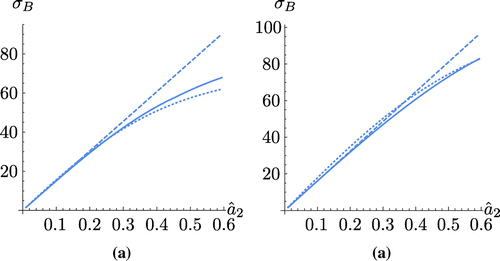
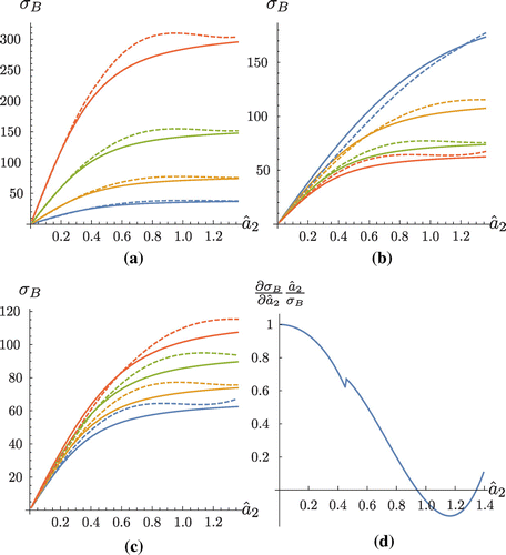
Figure 4. The maximum eigenvalues (approximated by Equation (50(50) $$\begin{array}{cc}\hfill {\mathit{\sigma }}_B({\widehat{a}}_2)& =(\widehat{A}+{\widehat{S}}_1({\widehat{a}}_2)){\widehat{a}}_2+{\widehat{S}}_2({\widehat{a}}_2){\widehat{a}}_2^3+Q({\widehat{a}}_2)cos(p({\widehat{a}}_2)-\mathit{\varphi }({\widehat{a}}_2)),\hfill \end{array}$$(50) ) (dashed) and obtained numerically from the scattering matrices arising from Equation (12(12) $$\begin{array}{c}\hfill A({\widehat{y}}_m,{\widehat{y}}_n)=\frac{\sqrt{1-{\widehat{y}}_m^2}}{\mathit{\rho }{c}^2|{\widehat{y}}_n+{\widehat{y}}_m|}(L+2\mathit{\mu }(1-{\widehat{y}}_n^2))J_1(2\mathit{\pi }{\widehat{a}}_2|{\widehat{y}}_n+{\widehat{y}}_m|)\end{array}$$(12) ) (full line) plotted against ${\widehat{a}}_2$ as (a) the number of elements changes ($N=32$ (blue), 64 (yellow), 128 (green) and 256 (orange), the array length is fixed at $l=128$ mm and depth at $d=50$ mm), (b) the array length varies ($l=32$ mm (blue), 64 mm (yellow), 128 mm (green) and 256 mm (orange), the number of elements is fixed at $N=64$ and depth at $d=50$ mm) and (c) the distance of the flaw from the array increases ($d=25$ mm (blue), 50 mm (yellow), 75 mm (green), 100 mm (orange), the number of elements and array length are fixed at $N=64$, $l=128$ mm). Plot (d) shows the relative partial derivative of ${\mathit{\sigma }}_B$ with respect to $\widehat{a}$.

4.2. Sensitivity to system parameters

In order to assess the robustness of this approximation, a comparison with the numerically calculated maximum eigenvalue from the original scattering matrix (given by Equation (12(12) $$\begin{array}{c}\hfill A({\widehat{y}}_m,{\widehat{y}}_n)=\frac{\sqrt{1-{\widehat{y}}_m^2}}{\mathit{\rho }{c}^2|{\widehat{y}}_n+{\widehat{y}}_m|}(L+2\mathit{\mu }(1-{\widehat{y}}_n^2))J_1(2\mathit{\pi }{\widehat{a}}_2|{\widehat{y}}_n+{\widehat{y}}_m|)\end{array}$$(12) )) was made as the system parameters were varied. It was shown that by increasing the number of elements N whilst keeping the array length constant ($l=128$ mm), an increase in the maximum eigenvalue was observed (see Figure 4(a)). This suggests that ${\mathit{\sigma }}_B$ is more sensitive to the size of the crack as the density of the array elements increases. The effect of varying the array pitch of the ultrasonic linear array (by allowing the array aperture l to increase whilst the number of elements remained fixed at $N=64$) was examined similarly (see Figure 4(b)) and reiterates that a higher density of elements is more beneficial than an increased linear aperture. Finally, the sensitivity of the maximum eigenvalue approximation to the distance between the array and the flaw was studied and it was shown that the greater the depth of the flaw relative to the array, the more sensitive the eigenvalue is to changes in the crack length (see Figure 4(c)). One benefit of obtaining the explicit expression for the maximum eigenvalue of the scattering matrix (over its numerical calculation) is that it permits analytical insight on the behaviour of the system parameters. For example, it allows us to examine the sensitivity of the maximum eigenvalue to the crack length at a set of fixed system parameters ($d=50$ mm, $N=64$ and $l=128$ mm) by calculating the partial derivative of ${\mathit{\sigma }}_B$ with respect to ${\widehat{a}}_2$. The results are plotted as ${\widehat{a}}_2$ is varied in Figure 4(d) and a discontinuity around ${\widehat{a}}_2\approx 0.5$ is observed. This can be attributed to the change in $t^{\ast }$ which is dependent on ${\widehat{a}}_2$ and determines whether the approximation for small or large arguments is used. It can be observed that ${\mathit{\sigma }}_B$ is particularly sensitive to changes in the crack radius to wavelength ratio when ${\widehat{a}}_2<0.5$. This suggests that the inverse problem of recovering ${\widehat{a}}_2$ from measured values of the maximum eigenvalue is viable when the crack length is commensurate with (or in the neighbourhood of) the wavelength. When this threshold is exceeded it is suggested that another technique, such as an image-based method (the Total Focussing Method (TFM) for example [11]) should be used.

5. Results from simulated data

In this section we apply the method to simulated FMC data generated using the finite element package PZFlex [31]. Note that although the mathematics derived in this paper is carried out in terms of the crack radius to wavelength ratio ${\widehat{a}}_2$, the following results will be discussed in terms of crack length to wavelength ratio, $\widehat{a}$, for consistency with the existing literature. The finite element package was used to simulate the ultrasonic phased array inspection of a homogeneous steel block containing a 5 mm crack lying parallel to the array at a depth of 50 mm, excited by a 1.5 MHz single cycle sinusoid (the parameters used in this simulation are given in Table 1). Within the finite element simulation, the domain was meshed with elements of dimension $\mathit{\lambda }/15$. With a centre frequency of 1.5 MHz, this gave an element size of approximately $200\mathrm{\mu }\mathrm{m}$, thus lying below the Rayleigh scattering limit of $300\mathrm{\mu }\mathrm{m}$ and so sufficient to model accurate wave propagation [32]. Each resulting transmit-receive time domain signal was transformed into the frequency domain using a Fast Fourier Transform. A $-3$ dB window was taken around the 1.5 MHz central frequency to give a usable bandwidth of $0.75-2.25$ MHz giving rise to a range of 0.6 to 1.9 for the crack length to wavelength ratio, $\widehat{a}=2a_2/\mathit{\lambda }$ (or alternatively the crack radius to wavelength ratio range is $0.3<{\widehat{a}}_2<0.95$). The simulation included a number of effects which are not taken into account by the Kirchhoff model. For example, in the Kirchhoff model the effects of mode conversion are neglected; only a pressure wave is considered. The discrepancies between the model and simulation result in an amplitude difference and therefore the scattering matrices were necessarily normalized. The scattering matrices from the simulated data, $A_S(m,n,f)$, and from the model, $A_K(m,n,a,f)$, (where $m,n=1,\dots ,N$ correspond to transmitting and receiving element indices) were normalized with respect to the $l_2$-norm to allow the signatures of each to be compared as the crack length, a, and frequency, f were varied. We let ${\mathit{\sigma }}_S(f)$ denote the numerically calculated maximum eigenvalue from the normalized scattering matrix arising from the simulation, at a frequency, f, and ${\mathit{\sigma }}_K(a,f)$ denote the numerically calculated maximum eigenvalue from the normalized matrix arising from the Kirchhoff model at frequency f and crack length a. The differences between ${\mathit{\sigma }}_S(f)$ and ${\mathit{\sigma }}_K(a,f)$ are summed over the frequency range as the crack length a is varied,(52) $$\begin{array}{c}\hfill D(a)=||{\mathit{\sigma }}_S(f)-{\mathit{\sigma }}_K(a,f){||}_2,\end{array}$$(52)

where D(a) is the objective function (based on the $L_2$ norm whereby the difference between the measured and modelled spectra is integrated over the frequency range of interest) for which we are seeking the value of a for which the global minimum is obtained. Figure 5 plots D(a) as the crack length a is varied within the model and shows a clear global minimum for $a=4.4$ mm (there is therefore no uniqueness issue to concern us here). 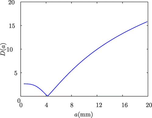The actual crack length in the simulation is 5 mm and so the percentage error in the value recovered using the maximum eigenvalue method is $12\%$, which is a reasonable error considering the assumptions within the model and the effects within the simulation which are not included within the model.

Table 1. Parameters used in the finite element simulation of the ultasonic phased array inspection of a homogeneous medium with a horizontal crack inclusion.

Ultrasonic transducer array parameters	Value	Units
Number of elements	64	–
Pitch	2	mm
Element width	1.5	mm
Transducer centre frequency	1.5	MHz
Array length	128	mm
Wave speed in host material	5900	ms${}^{-1}$
Density of host material	7890	kg/m${}^3$
Flaw length	5	mm
Depth of flaw	50	mm
Depth of sample	78.6	mm
Time sample rate	17.3	ns

Figure 5. This plot shows D(a) from Equation (52(52) $$\begin{array}{c}\hfill D(a)=||{\mathit{\sigma }}_S(f)-{\mathit{\sigma }}_K(a,f){||}_2,\end{array}$$(52) ), integrated over a range of frequencies (0.75–2.25 MHz) comparing the maximum eigenvalues from the scattering matrices from the simulated data, ${\mathit{\sigma }}_S(f)$, and the Kirchhoff model, ${\mathit{\sigma }}_K(a,f)$, as the crack length, a, is varied within the model.

6. Discussion

The method proposed in this paper presents a novel approach for the sizing of subwavelength cracks. Typically, within the non-destructive evaluation industry, flaw characterisation is secondary to detection and takes place at the imaging stage, where some threshold is applied to an image (perhaps generated by the TFM) and groups of pixels lying above this threshold are used to measure the flaw dimensions. This can be problematic on two levels: firstly, there is no standardized procedure for sizing subwavelength defects and so estimations are subjective and may vary between companies and operators; secondly, it is difficult to automate this type of measurement. The method presented here is a completely objective approach which could potentially supplement existing methods. And so, once a time domain image has been constructed, time windows containing defect scattering can be identified and transformed into the frequency domain and scattering matrices can thus be generated. Once at this stage, the method implemented in Section 5 can be applied autonomously and an objective crack size measurement can thus be obtained. It must be mentioned that scattering matrices have already been exploited for objective crack sizing in [19–21]. However, the benefit of the method proposed here is that the generation of reference scattering matrices for comparison with those arising from the data is negated and instead only the calculation of a single value is required, which is computationally more efficient. The inversion process implemented in Section 5 relies on the comparison of the maximum eigenvalues of scattering matrices arising from the observed data with maximum eigenvalues arising from a model based on the known experimental parameters (host medium properties, array configuration etc.) integrated over a range of frequencies determined by the transducer’s bandwidth. There are two ways to calculate these model eigenvalues: either by generating model scattering matrices using the Kirchhoff approximation, numerically obtaining the eigenvalues and taking the maximum, or by using the explicit expression for the maximum eigenvalue as presented in this paper. To demonstrate the computational benefits of this approach, we can compare the computation times taken to generate Figure 3(a) using Mathematica. Here, the numerical approach (which involved generating the scattering matrix and then calculating the eigenvalues numerically – dotted line) took $\mathcal{O}(10)$ seconds. Evaluating equation (50) over the entire range of ${\widehat{a}}_2$ (full line) took only $\mathcal{O}(1)$ seconds. Furthermore, the linear approximation (dashed line) took only $\mathcal{O}({10}^{-2})$ seconds, almost ${10}^3$ times faster. This improvement is advantageous for the inversion process as these calculations are repeated over a large range of crack lengths and frequencies, and thus the saving in computational time is magnified. Finally, it must be noted that attention was restricted to cracks which lie parallel to the ultrasonic array in this paper. To study the effects of crack orientation, one could relax this assumption but as this adds significantly to the complexity of the formulation this remains future work.

7. Conclusions

In this paper a formula which relates the maximum eigenvalue from a scattering matrix to the length of a crack within an elastic solid was presented. This formula shows that there is a one to one relationship between the two and that this can be used to tackle the inverse problem of objectively sizing a crack in an elastic solid given the ultrasonic array output data. The Kirchhoff model was used to approximate the scattering matrices which arise when a linear elastic wave encounters a crack within a homogeneous medium. By restricting our attention to cracks lying parallel to the array, the scattering matrix from the model was approximated by a Toeplitz matrix and an upper bound to the maximum eigenvalue from this Toeplitz matrix was used to derive an explicit relationship between the maximum eigenvalue and the crack radius to wavelength ratio, ${\widehat{a}}_2=a_2/\mathit{\lambda }$. The sensitivity of the maximum eigenvalue approximation, ${\mathit{\sigma }}_B$, to changes in the system parameters was also examined. From this analysis it was concluded that ${\mathit{\sigma }}_B$ is most sensitive to changes in ${\widehat{a}}_2$ when ${\widehat{a}}_2<0.5$ and that there is little change in ${\mathit{\sigma }}_B$ for ${\widehat{a}}_2>0.5$. This implies that the method of using the maximum eigenvalue to determine the size of a crack in a homogeneous material (the inverse problem) is most effective when the crack is of similar length to the wavelength (that is, when ${\widehat{a}}_2\approx 0.5$). For larger cracks, it is recommended that another method is adopted, such as an image-based method (for example the TFM). The method was applied to time domain FMC data from a finite element simulation and the crack size was objectively recovered exhibiting an error of $12\%$. Aside to providing an entirely objective crack size estimate, the method is advantageous over other scattering matrix approaches in that it does not require the generation of reference scattering matrices for comparison with the data, only the calculation of a single value is required. For the simple case presented in this paper, our approach was up to ${10}^3$ times faster than numerically modelling the scattering matrix and obtaining its eigenvalues.

Additional information

Funding

This work was funded by the Engineering and Physical Sciences Research Council [grant number EP/P505747/1]; Doosan Babcock.

Notes

No potential conflict of interest was reported by the authors.

References

- Hellier C. Handbook of nondestructive evaluation. New York (NY): McGraw Hill Professional; 2012.
- Adams R, Cawley P. A review of defect types and non destructive testing techniques for composites and bonded joints. NDT & E Int. 1988;21(4):208–222.
- Cheng L, Tian G. Pulsed electromagnetic NDE for defect detection and characterisation in composites. In: IEEE I2MTC. Graz, Austria; 2012 May 13--16.
- Ettemeyer A. Laser shearography for inspection of pipelines. Nucl Eng Des. 1996;160:237–240.
- Rose J. Ultrasonic waves in solid media. Cambridge: Cambridge University Press; 1999.
- Schmerr L, Song S. Ultrasonic nondestructive evaluation systems. (NY): Springer; 2010.
- Safari A, Akdogan E. Piezoelectric and acoustic materials for transducer applications. New York (NY): Springer Science + Business Media; 2008.
- Drinkwater B, Wilcox P. Ultrasonic arrays for non-destructive evaluation: a review. NDT & E Int. 2006;39(7):525–541.
- Connolly G, Lowe M, Rokhlin S, et al. Imaging of defects within austenitic steel welds using an ultrasonic array. In: Leger A, Deschamps M, editors. Ultrasonic wave propagation in non homogeneous media. Berlin: Springer-Verlag; 2009. p. 25–38.
- Velichko A, Wilcox P. An analytical comparison of ultrasonic array imaging algorithms. JASA. 2010;127(4):2378–2384.
- Holmes C, Drinkwater B, Wilcox P. Post processing of the full matrix of ultrasonic transmit receive array data for non destructive evaluation. NDT & E Int. 2005;38(8):701–711.
- Wilcox P, Holmes C, Drinkwater B. Advanced reflector characterization with ultrasonic phased arrays in NDE applications. IEEE TUFFC. 2005;38(8):701–711.
- Kirsch A, Grinberg N. The factorization method for inverse problems. Oxford: Oxford University Press; 2008.
- Colton D, Kirsch A. A simple method for solving inverse scattering problems in the resonance region. Inverse Prob. 1996;12(4):383.
- Kress R, Rundell W. Inverse scattering for shape and impedance. Inverse Prob. 2001;17(4):1075.
- Achenbach JD, Viswanathan K, Norris A. An inversion integral for crack-scattering data. Wave Motion. 1979;1(4):299–316.
- Chapman R. A system model for the ultrasonic inspection of smooth planar cracks. J Nondestructive Eval. 1990;9(2–-3):197–210.
- Kitahara M, Nakahata K, Hirose S. Elastodynamic inversion for shape reconstruction and type classification of flaws. Wave Motion. 2002;36(4):443–455.
- Tant KMM, Mulholland AJ, Gachagan A. A model-based approach to crack sizing with ultrasonic arrays. IEEE TUFFC. 2015;62(5):915–926.
- Zhang J, Drinkwater B, Wilcox P. The use of ultrasonic arrays to characterize crack-like defects. J Nondestructive Eval. 2010;29(4):222–232.
- Bai L, Velichko A, Drinkwater B. Ultrasonic characterization of crack-like defects using scattering matrix similarity metrics. IEEE TUFFC. 2015;62(3):545–559.
- Schmerr L. Fundamentals of ultrasonic nondestructive evaluation: a modelling approach. New York (NY): Plenum Press; 1998.
- Böttcher A, Grudsky SM. Spectral properties of banded toeplitz matrices. Philadelphia: SIAM; 2005.
- Böttcher A, Grudsky SM. Toeplitz matrices, asymptotic linear algebra, and functional analysis. Basel: Birkhäuser; 2012.
- Gray R. On the asymptotic eigenvalue distribution of toeplitz matrices. IEEE Trans Inform Theory. 1972;18(6):725–730.
- Reichel L, Trefethen LN. Eigenvalues and pseudo-eigenvalues of toeplitz matrices. Linear Algebra Appl. 1992;162:153–185.
- Hertz D. Simple bounds on the extreme eigenvalues of toeplitz matrices. IEEE Trans Inform Theory. 1992;38(1):175–176.
- Abramowitz M, Stegun I. Handbook of mathematical functions with formulas, graphs and mathematical tables. New York (NY): Dover; 1972.
- Cunningham L. Mathematical model based methods for characterising defects within ultrasonic non destructive evaluation [dissertation]. Glasgow: The University of Strathclyde; 2015.
- Arakawa T, Ibukiyama T, Kaneko M, et al. Bernoulli numbers and zeta functions. Tokyo: Springer; 2014.
- PZFlex. Thornton Tomasetti Defence Ltd 6th Floor South, 39 St Vincent Place, Glasgow, Scotland, G1 2ER, United Kingdom; 2016.
- Harvey G, Tweedie A, Carpentier C, et al. Finite element analysis of ultrasonic phased array inspections on anisotropic welds. In: AIP Conference Proceedings, Vol. 1335. San Diego, CA; 2010. p. 827–834.