Trace formula and inverse nodal problem for a conformable fractional Sturm-Liouville problem

ABSTRACT

In this paper, we have developed the spectral theory for a conformable fractional Sturm-Liouville problem $L_{\alpha }\left(q\right(x),h,H)$ with boundary conditions which include conformable fractional derivatives of order α, $0<\alpha ⩽1$, and prove a completeness theorem and an expansion theorem. We obtain the canonical infinite product constructed by the zero set of the characteristic function of $L_{\alpha }$. Also, we calculate the regularized trace formula of the eigenvalues and investigate the inverse nodal problem for this problem with real-valued coefficients on a finite interval. The oscillation of the eigenfunctions for sufficiently large n is established, and an asymptotic formula for elements constructed by of nodal points is obtained. The uniqueness theorem is proved, and an effective procedure for solving the inverse problem is given. Finally, we present two examples to illustrate our theoretical findings.

KEYWORDS:

• Sturm-Liouville problem
• conformable fractional derivatives and integrals
• infinite product representation
• eigenfunctions
• eigenvalues
• trace formula
• inverse nodal problems
• expansion theorem
• nodal points
• reconstruction formula

JEL CLASSIFICATIONS:

• 34B24
• 34A08
• 34A55
• 47E05
• 34L10
• 34L20
• 26A33

1. Introduction

The beginning of the fractional calculus is considered to be Leibniz's letter to L'Hôspital in 1695. L'Hôspital asked, ‘what does it mean $\frac{{\mathrm{d}}^{n}f}{\mathrm{d}{x}^n}$ if $n=\frac{1}{2}$?’. Since then, various types of fractional derivatives have been introduced, most of which use an integral form with different singular kernels for the fractional derivative. Due to the same reason, these fractional derivatives inherit some non-local behaviours which lead them to numerous interesting applications, including memory effects and future dependence. However, almost all the fractional derivatives used in this literature, such as Grünwald-Letnikov, Riemann-Liouville, Caputo and Jumarie, Marchaud and Riesz, fail to satisfy some of the basic properties owned by usual derivatives, e.g. the product rule, chain rule, Rolle's theorem, mean value theorem, composition rule and semigroup property. These inconsistencies lead to the development of the local fractional derivative whose most properties coincide with classical integer derivative. Recently, Khalil, Al Horani, Yousef and Sababhehb [1] introduced a new local fractional derivative and fractional integral. This simple, well-behaved definition enables us to prove many properties analogous to those of integer-order derivative, probably because it includes a limit, instead of an integral. More basic properties and main results on conformable derivative can be found in [2,3]. Despite the numerous attractive properties the conformable derivative has, it has drawbacks and some unusual properties, e.g. the zero order derivative of a function does not return the function and the index law does not hold, that is, $D^{\alpha }{D}^{\beta }f\left(t\right)\ne D^{\alpha +\beta }f\left(t\right)$ for any α and β. Some authors (See [4]) have argued that conformable fractional derivative is not a truly fractional operator. This question seems today to still be open and perhaps it is a philosophical issue. Because of its effectiveness and applicability, conformable derivative has been employed in various field such as the control theory of dynamical systems [5], Newton mechanics [6,7], quantum mechanics [8], variational calculus [9], arbitrary time scale problems [10,11], anomalous diffusion [12], diffusive transport [13,14] and stochastic process [15]. Recently, a physical interpretation of the conformable derivative is provided by Zhao and Luo [16]. They generalized the definition of the conformable derivative to general conformable derivative by means of linear extended $G\hat{a}teaux$ derivative, and used this definition to demonstrate that the physical interpretation of the conformable derivative is a modification of classical derivative in direction an dmagnitude. So, in our opinion, the interest in the conformable derivative has been increasing and it is worthwhile to explore in this new research area.

In recent years, much effort has focussed on a fractional generalization of the well-known Sturm-Liouville problems (See [17–20]). Fractional Sturm-Liouville problems (FSLPs) are different from those usually defined in this literature, i.e. the ordinary derivatives in a traditional Sturm-Liouville problem are replaced with fractional derivatives or derivatives of fractional order. These types of FSLPs arise in various areas of science and in many fields in engineering, we refer to [21–25]. Now, we consider on the closed interval $[0,\pi ]$ the boundary value problem $L_{\alpha }\left(q\right(x),h,H)$: (1) ${\ell }_{\alpha }y:=-D_x^{\alpha }{D}_x^{\alpha }y+q\left(x\right)y=\lambda y,0<x<\pi ,$(1) with boundary conditions (2) $U\left(y\right):=D_x^{\alpha }y\left(0\right)-hy\left(0\right)=0,V\left(y\right):=D_x^{\alpha }y\left(\pi \right)+Hy\left(\pi \right)=0,$(2) known as a conformable fractional Sturm-Liouville problem (CFSLP). Here, λ is the spectral parameter, $q\left(x\right)$, h and H are real, and $q\left(x\right)\in L_{\alpha }^2(0,\pi )$. Where $D_x^{\alpha }$ is the CF derivative of order α, $0<\alpha \le 1$. The operator ${\ell }_{\alpha }$ is called the CFSL operator.

The present paper is composed of two main parts. In the first part, we prove the existence of infinitely many real eigenvalues of the CFSLP which are simple, and that the corresponding eigenfunctions are orthogonal (See parts 1, 2 and 3 of Theorem 3.7), and then, we provide the asymptotic behaviour of eigenvalues and the corresponding eigenfunctions (Theorem 3.10). The proof concerning the expansion theorem is established by means of contour integration and the calculus of residues (Theorem 3.12). Also, we obtain the canonical infinite product constructed by the zero set of the characteristic function of $L_{\alpha }$ (Theorem 3.11). Then, we present an explicit formula of the regularized trace regarding the boundary condition parameters and the potential for the problem (1(1) ${\ell }_{\alpha }y:=-D_x^{\alpha }{D}_x^{\alpha }y+q\left(x\right)y=\lambda y,0<x<\pi ,$(1) )–(2(2) $U\left(y\right):=D_x^{\alpha }y\left(0\right)-hy\left(0\right)=0,V\left(y\right):=D_x^{\alpha }y\left(\pi \right)+Hy\left(\pi \right)=0,$(2) ) by using Levitan's method as in [26] (See Theorem 4.3). The study of regularized traces for the Sturm-Liouville operator on a finite interval was initiated in [27]. Later on, some authors turned their attention to trace theory and obtained exciting results [28–31]. This research continued in many respects, such as Dirac operators, the matrix Schrödinger equation with energy-dependent potential, the linear damped wave equation, differential operators with abstract operator-valued coefficients, and the case of matrix-valued Sturm-Liouville operators, etc. (See for instance, [32–36]). In the second part, we investigate the inverse nodal problem for the CFSLP (1(1) ${\ell }_{\alpha }y:=-D_x^{\alpha }{D}_x^{\alpha }y+q\left(x\right)y=\lambda y,0<x<\pi ,$(1) ) with boundary conditions (2(2) $U\left(y\right):=D_x^{\alpha }y\left(0\right)-hy\left(0\right)=0,V\left(y\right):=D_x^{\alpha }y\left(\pi \right)+Hy\left(\pi \right)=0,$(2) ) which includes the CF derivative of order α, $0<\alpha ⩽1$. At first, we obtain a detailed asymptotic formula for elements constructed by of nodal points (Lemma 5.1). Then, we demonstrate that the n-th eigenfunction of $L_{\alpha }$ has precisely n nodes in the interval $(0,\pi )$ for sufficiently large n, which is an analogue of the classical Sturm's oscillation theorem for the Sturm-Liouville operator (Theorem 5.2). Further, we prove a uniqueness theorem and provide two algorithms to reconstruct the potential function q and the parameters h, H in the boundary conditions from elements constructed by of nodes and the length of those elements (See Theorem 5.5 and Theorem 5.9). The inverse nodal problem, which is different from the classical inverse spectral theory of Gelfand and Levitan [37], was started by McLaughlin [38]. Later, Hald and McLaughlin [39] and Browne and Sleeman [40] proved that it is sufficient to know the nodal points to determine the potential function of the regular Sturm-Liouville problem uniquely. Yang [41] presented an algorithm to recover q from a dense subset of nodal points. Furthermore, the inverse nodal Sturm-Liouville problems have been considered recently in [42–48].

This paper is organized as follows. In Section 2 some basic definitions and properties of CF calculus are given. Section 3 is devoted to the study of the spectrum of the CFSL operator. The regularized traces for the ${\ell }_{\alpha }$ operator with boundary conditions is calculated in Section 4. Our main results are given in Section 5. We discuss the inverse nodal problem of reconstructing the potential from an arbitrary dense set of elements constructed by of nodes of the boundary value problem $L_{\alpha }$. Finally, we summarize our results in Section 6.

2. Conformable fractional preliminaries

Here, we give some basic definitions and properties of the conformable fractional calculus theory which can be found in [1,2].

Definition 2.1

Let $f:[0,\mathrm{\infty })\to \mathbb{R}$ be a given function. Then, the conformable fractional derivative of f of order α is defined by: (3) $D^{\alpha }f\left(x\right)=\underset{h\to 0}{lim}\frac{f(x+h{x}^{1-\alpha })-f\left(x\right)}{h},D^{\alpha }f\left(0\right)=\underset{x\to 0^{+}}{lim}{D}^{\alpha }f\left(x\right),$(3) for all $x>0,\alpha \in (0,1]$. Note that if f is differentiable, then (4) $D^{\alpha }f\left(x\right)=x^{1-\alpha }{f}^{\prime }\left(x\right),$(4) where $f^{\prime }\left(x\right)=\underset{h\to 0}{lim}\left[f\right(x+h)-f(x\left)\right]/h$. If $D^{\alpha }f\left(x_0\right)$ exists and is finite, we say that f is α-differentiable at $x_0$. From now on, assume that $D_x^{\alpha }\equiv D^{\alpha }$ (i.e. the CF derivative of order α with respect to x).

Theorem 2.2

If a function $f:[0,\mathrm{\infty })\to \mathbb{R}$ is α-differentiable at $x_0>0$. Then, f is continuous at $x_0$.

Definition 2.3

Let $f:[0,\mathrm{\infty })\to \mathbb{R}$ be a given function. Then, the conformable fractional integral of f of order α is defined by: (5) $I_{\alpha }f\left(x\right)={\int }_0^{x}f\left(t\right){\mathrm{d}}_{\alpha }t={\int }_0^x{t}^{\alpha -1}f\left(t\right)\mathrm{d}t,$(5) for all $x>0$. Where the integral is the usual Riemann improper integral.

Theorem 2.4

Let f, g be α-differentiable at x, x>0. Then

1. $D_x^{\alpha }(af+bg)=a{D}_x^{\alpha }f+b{D}_x^{\alpha }g,$ $\mathrm{\forall }a,b\in \mathbb{R},$

2. $D_x^{\alpha }\left(x^p\right)=p{x}^{p-\alpha },$ $\mathrm{\forall }p\in \mathbb{R},$

3. $D_x^{\alpha }\left(c\right)=0,$ $($c is a constant$),$

4. $D_x^{\alpha }\left(fg\right)=D_x^{\alpha }\left(f\right)g+f{D}_x^{\alpha }\left(g\right),$

5. $D_x^{\alpha }\left(f/g\right)=\frac{D_x^{\alpha }\left(f\right)g-f{D}_x^{\alpha }\left(g\right)}{g^2}$.

Lemma 2.5

Let $f:[a,\mathrm{\infty })\to \mathbb{R}$ be any continuous function. Then, for all $x>a,$ we have $D_x^{\alpha }{I}_{\alpha }f\left(x\right)=f\left(x\right)$.

Lemma 2.6

Let $f:(a,b)\to \mathbb{R}$ be differentiable. Then, for all $x>a,$ we have $I_{\alpha }{D}_x^{\alpha }f\left(x\right)=f\left(x\right)-f\left(a\right).$

Theorem 2.7

α-chain rule

Let $f,g:(0,\mathrm{\infty })\to \mathbb{R}$ be α-differentiable functions and $h\left(x\right)=f\left(g\right(x\left)\right)$. Then, $h\left(x\right)$ is α-differentiable and for all $x(x\ne 0\mathrm{a}\mathrm{n}\mathrm{d}g(x)\ne 0)$ and $\left(D_x^{\alpha }h\right)\left(x\right)=\left(D_x^{\alpha }f\right)\left(g\right(x\left)\right).\left(D_x^{\alpha }g\right)\left(x\right).g(x{)}^{\alpha -1}.$ If $x=0,$ then $\left(D_x^{\alpha }h\right)\left(0\right)=\underset{x\to 0^{+}}{lim}\left(D_x^{\alpha }f\right)\left(g\right(x\left)\right).\left(D_x^{\alpha }g\right)\left(x\right).g(x{)}^{\alpha -1}$.

Proposition 2.8

Let $0<\alpha ,\beta \le 1$ such that $1<\alpha +\beta \le 2$ and f be a function defined on $[0,\mathrm{\infty })$. Then, the following semigroup properties hold:

1. If f be twice differentiable on $(0,\mathrm{\infty }),$ then $\left(D_x^{\alpha }{D}_x^{\beta }f\right)\left(x\right)=D_x^{\alpha +\beta }f\left(x\right)+(1-\beta )x^{-\beta }{D}_x^{\alpha }f\left(x\right).$

2. $\left(I_{\alpha }{I}_{\beta }f\right)\left(x\right)=\frac{x^{\beta }}{\beta }{I}_{\alpha }f\left(x\right)+\frac{1}{\beta }{I}_{\alpha +\beta }f\left(x\right)-\frac{x}{\beta }{\int }_0^x{t}^{\alpha +\beta -2}f\left(t\right)\mathrm{d}t$.

Note that if $\alpha ,\beta \to 1,$ then $\left(D^1{D}^{1}f\right)\left(x\right)=D^{2}f\left(x\right)=f^{″}\left(x\right),$ $\left(I_1{I}_{1}f\right)\left(x\right)=I_{2}f\left(x\right)$.

Theorem 2.9

α-integration by parts

Let $f,g:[a,b]\to \mathbb{R}$ be two functions such that fg is differentiable. Then (6) ${\int }_a^{b}f\left(x\right)D_x^{\alpha }g\left(x\right){\mathrm{d}}_{\alpha }x=fg{|}_a^b-{\int }_a^{b}g\left(x\right)D_x^{\alpha }f\left(x\right){\mathrm{d}}_{\alpha }x.$(6)

Definition 2.10

The space $C_{\alpha }^n[a,b]$ consists of all functions defined on the interval $[a,b]$ which are continuously α-differentiable up to order n.

Definition 2.11

Let $1\le p<\mathrm{\infty }$, $a>0$. The space $L_{\alpha }^p(0,a)$ consists of all functions $f:[0,a]\to \mathbb{R}$ satisfying the condition $\left({\int }_0^a\right|f\left(x\right){|}^p{\mathrm{d}}_{\alpha }x{)}^{1/p}<\mathrm{\infty }$.

Lemma 2.12

The space $L_{\alpha }^p(0,a)$ associated with the norm function $\parallel f{\parallel }_{p,\alpha }:={\left({\int }_0^a\left|f\right(x){|}^p{\mathrm{d}}_{\alpha }x\right)}^{1/p},$ is a Banach space. Moreover, if $p=2,$ then $L_{\alpha }^2(0,a)$ associated with the inner product $⟨f,g⟩:={\int }_0^{a}f\left(x\right)\overline{g\left(x\right)}{\mathrm{d}}_{\alpha }x,(f,g\in L_{\alpha }^2(0,a\left)\right),$ is a Hilbert space $($See [49]).

Definition 2.13

Let $p\in \mathbb{R}$ be such that $p\ge 1$. The Sobolev space $W_{\alpha }^p(0,a)$ consists of all functions defined on the interval $[0,a]$, such that $f\left(x\right)$ is absolutely continuous, and $D_x^{\alpha }f\left(x\right)\in L_{\alpha }^p(0,a)$ (See [49] for more details).

Lemma 2.14

α-Leibniz rule

Let $t^{\alpha -1}f(x,t)$ and $t^{\alpha -1}{f}_x(x,t)$ be continuous in x on some regions of the $(x,t)$-plane, including $a\left(x\right)\le t\le b\left(x\right),x_0\le x\le x_1$. If $a\left(x\right)$ and $b\left(x\right)$ are both α-differentiable for $x_0\le x\le x_1,$ then $\begin{array}{rl}{D}_x^{\alpha }\left[{\int }_{a\left(x\right)}^{b\left(x\right)}f(x,t){\mathrm{d}}_{\alpha }t\right]& =D_x^{\alpha }b\left(x\right)f(x,b(x\left)\right)b(x{)}^{\alpha -1}-D_x^{\alpha }a(x\left)f\right(x,a\left(x\right)\left)a\right(x{)}^{\alpha -1}\\ & +{\int }_{a\left(x\right)}^{b\left(x\right)}{D}_x^{\alpha }f(x,t){\mathrm{d}}_{\alpha }t.\end{array}$

Proof.

From the Leibniz rule, the proof is clear.

Lemma 2.15

Assume that $u\left(x\right)$ and $v\left(x\right)$ be real-valued, nonnegative on an interval $[0,\pi ],$ $u\left(x\right)$ is a continuous function, and $v\left(x\right)\in L_{\alpha }(0,\pi )$. If $u\left(x\right)\le c+{\int }_0^{x}v\left(x\right)u\left(x\right){\mathrm{d}}_{\alpha }t,$ where c is a non negative constant, then $u\left(x\right)\le c\exp \left({\int }_0^{x}v\right(x\left){\mathrm{d}}_{\alpha }t\right)$.

Proof.

This lemma can be proved by using an argument similar to that for Lemma 3.2.1. in [30].

3. Conformable fractional Sturm-Liouville problems

In this section, we collect known results about the spectra of the regular conformable fractional Sturm-Liouville operator on a finite interval. Note that more general second-order equations (7) $D_x^{\alpha }\left[p\left(x\right)D_x^{\alpha }y\right]+\left\{l\right(x)+\lambda r(x\left)\right\}y=0,0<\alpha \le 1,$(7) where the function $r\left(x\right)$ is positive on $[a,b]$, are reducible to the form (1(1) ${\ell }_{\alpha }y:=-D_x^{\alpha }{D}_x^{\alpha }y+q\left(x\right)y=\lambda y,0<x<\pi ,$(1) ). If we assume that $r\left(x\right)\in C_{\alpha }^2[a,b]$ and $p\left(x\right)\in C_{\alpha }^1[a,b]$, then (7(7) $D_x^{\alpha }\left[p\left(x\right)D_x^{\alpha }y\right]+\left\{l\right(x)+\lambda r(x\left)\right\}y=0,0<\alpha \le 1,$(7) ) by the change of variables such as those of Joseph Liouville (8) $\frac{t^{\alpha }}{\alpha }={\int }_0^x\sqrt{r\left(s\right)}{\mathrm{d}}_{\alpha }s,w\left(t\right)=y\left(x\right)\sqrt[4]{r\left(x\right)}\exp \left(\frac{1}{2}{\int }_0^{x}p\left(s\right){\mathrm{d}}_{\alpha }s\right),$(8) can be reduced to the canonical form $-D_t^{\alpha }{D}_t^{\alpha }w+q\left(t\right)w=\lambda w$, where $q\left(t\right)=\frac{D_x^{\alpha }{D}_x^{\alpha }r\left(x\right)}{4r^2\left(x\right)}-\frac{5}{16}\frac{\left(D_x^{\alpha }r\right(x){)}^2}{r^3\left(x\right)}-\frac{1}{r\left(x\right)}\left[l\left(x\right)+\frac{1}{2}{D}_x^{\alpha }p\left(x\right)+\frac{1}{4}{p}^2\left(x\right)\right].$

3.1. Basic properties of the operator

Definition 3.1

Let $y\left(x\right),z\left(x\right)$ be α-differentiable functions on $[0,\pi ]$. The fractional Wronskian of y and z is defined as: (9) $W_{\alpha }[y,z]:=\left|\begin{array}{cc}y\left(x\right)& z\left(x\right)\\ D_x^{\alpha }y\left(x\right)& D_x^{\alpha }z\left(x\right)\end{array}\right|=y\left(x\right)D_x^{\alpha }z\left(x\right)-z\left(x\right)D_x^{\alpha }y\left(x\right).$(9)

Lemma 3.2

Two solutions y, z of Equation (1(1) ${\ell }_{\alpha }y:=-D_x^{\alpha }{D}_x^{\alpha }y+q\left(x\right)y=\lambda y,0<x<\pi ,$(1) ) defined an $(0,\pi )$ are linearly independent if and only if $W_{\alpha }[y,z]\left(x\right)\ne 0$ for all $x\in (0,\pi )$ $($See [50]).

Theorem 3.3

For $c_1,c_2\in \mathbb{C},$ Equation (1(1) ${\ell }_{\alpha }y:=-D_x^{\alpha }{D}_x^{\alpha }y+q\left(x\right)y=\lambda y,0<x<\pi ,$(1) ) has a unique solution in $C_{\alpha }^2[0,\pi ]$ which satisfies (10) $\varphi (0,\lambda )=c_1,D_x^{\alpha }\varphi (0,\lambda )=c_2,(\lambda \in \mathbb{C}).$(10) Moreover, $\varphi (x,\lambda )$ is an entire function of λ for all $x\in [0,\pi ]$.

Proof.

The proof of this theorem is provided in Appendix A.1.

Let $\varphi (x,\lambda ),\psi (x,\lambda )$ be the solutions of (1(1) ${\ell }_{\alpha }y:=-D_x^{\alpha }{D}_x^{\alpha }y+q\left(x\right)y=\lambda y,0<x<\pi ,$(1) ) under the conditions (11) $\varphi (0,\lambda )=1,D_x^{\alpha }\varphi (0,\lambda )=h,\psi (\pi ,\lambda )=1,D_x^{\alpha }\psi (\pi ,\lambda )=-H.$(11) Clearly, (12) $U\left(\varphi \right):=D_x^{\alpha }\varphi (0,\lambda )-h\varphi (0,\lambda )=0,V\left(\psi \right):=D_x^{\alpha }\psi (\pi ,\lambda )+H\psi (\pi ,\lambda )=0.$(12) We denote (13) $\mathrm{\Delta }\left(\lambda \right)=W_{\alpha }\left[\psi \right(x,\lambda ),\varphi (x,\lambda \left)\right].$(13) Using the formula for the fractional Wronskian (See [51]), $W_{\alpha }[y,z]\left(x\right)=W_{\alpha }[y,z]\left(x_0\right)$, $x\in (0,\pi )$, for two solutions y and z of (1(1) ${\ell }_{\alpha }y:=-D_x^{\alpha }{D}_x^{\alpha }y+q\left(x\right)y=\lambda y,0<x<\pi ,$(1) ) and some $x_0\in (0,\pi )$. Hence, $W_{\alpha }\left[\psi \right(x,\lambda ),\varphi (x,\lambda \left)\right]$ does not depend on x. The function $\mathrm{\Delta }\left(\lambda \right)$ is called the characteristic function of $L_{\alpha }$. Now, putting $x=0$ and $x=\pi$ in (13(13) $\mathrm{\Delta }\left(\lambda \right)=W_{\alpha }\left[\psi \right(x,\lambda ),\varphi (x,\lambda \left)\right].$(13) ), we get (14) $\mathrm{\Delta }\left(\lambda \right)=V\left(\varphi \right)=-U\left(\psi \right).$(14)

Theorem 3.4

The zeros $\left\{{\lambda }_n\right\}$ of the characteristic function coincide with the eigenvalues of the boundary value problem $L_{\alpha }$. The functions $\varphi (x,{\lambda }_n)$ and $\psi (x,{\lambda }_n)$ are eigenfunctions and there exists a sequence $\left\{{\beta }_n\right\}$ such that (15) $\psi (x,{\lambda }_n)={\beta }_n\varphi (x,{\lambda }_n),{\beta }_n\ne 0.$(15)

Proof.

The proof is very similar to the one proved in [52, Theorem 1.1.1.] and thus omitted.

Lemma 3.5

Denote ${\alpha }_n=\parallel \varphi (x,{\lambda }_n){\parallel }_{2,\alpha }^2$. Then, we have ${\beta }_n{\alpha }_n=-\dot{\mathrm{\Delta }}\left({\lambda }_n\right),$ where the numbers ${\beta }_n$ are defined by (15(15) $\psi (x,{\lambda }_n)={\beta }_n\varphi (x,{\lambda }_n),{\beta }_n\ne 0.$(15) ), and $\dot{\mathrm{\Delta }}\left(\lambda \right)=\frac{\mathrm{d}}{\mathrm{d}\lambda }\mathrm{\Delta }\left(\lambda \right)$. The data $\{{\lambda }_n,{\alpha }_n\}$ are called the spectral data of $L_{\alpha }$.

Proof.

Since $\begin{array}{rl}& -D_x^{\alpha }{D}_x^{\alpha }\psi (x,\lambda )+q\left(x\right)\psi (x,\lambda )=\lambda \psi (x,\lambda ),\\ & -D_x^{\alpha }{D}_x^{\alpha }\varphi (x,{\lambda }_n)+q\left(x\right)\varphi (x,{\lambda }_n)={\lambda }_n\varphi (x,{\lambda }_n),\end{array}$ we get $D_x^{\alpha }{W}_{\alpha }\left[\psi \right(x,\lambda ),\varphi (x,{\lambda }_n\left)\right]=(\lambda -{\lambda }_n)\psi (x,\lambda )\varphi (x,{\lambda }_n)$. Now, the α-integration over the interval $[0,\pi ]$ and using (5(5) $I_{\alpha }f\left(x\right)={\int }_0^{x}f\left(t\right){\mathrm{d}}_{\alpha }t={\int }_0^x{t}^{\alpha -1}f\left(t\right)\mathrm{d}t,$(5) ) and (14(14) $\mathrm{\Delta }\left(\lambda \right)=V\left(\varphi \right)=-U\left(\psi \right).$(14) ), we obtain $\begin{array}{rl}& (\lambda -{\lambda }_n){\left.{\int }_0^{\pi }\psi (x,\lambda )\varphi (x,{\lambda }_n){\mathrm{d}}_{\alpha }x=W_{\alpha }\left[\psi (x,\lambda ),\varphi (x,{\lambda }_n)\right]\right|}_0^{\pi }\\ & =D_x^{\alpha }\varphi (\pi ,{\lambda }_n)+H\varphi (\pi ,{\lambda }_n)+D_x^{\alpha }\psi (0,\lambda )-h\psi (0,\lambda )=-\mathrm{\Delta }\left(\lambda \right).\end{array}$ For $\lambda \to {\lambda }_n$, this yields ${\int }_0^{\pi }\psi (x,{\lambda }_n)\varphi (x,{\lambda }_n){\mathrm{d}}_{\alpha }x=-\underset{\lambda \to {\lambda }_n}{lim}\frac{\mathrm{\Delta }\left(\lambda \right)}{\lambda -{\lambda }_n}=-\dot{\mathrm{\Delta }}\left({\lambda }_n\right)$. Using (15(15) $\psi (x,{\lambda }_n)={\beta }_n\varphi (x,{\lambda }_n),{\beta }_n\ne 0.$(15) ) and ${\alpha }_n$ concludes the proof.

Lemma 3.6

Let $\alpha \in (0,1]$. Then the CFSL operator ${\ell }_{\alpha }$ is a self-adjoint on $L_{\alpha }^2(0,\pi )$. In other words, (16) $⟨{\ell }_{\alpha }u,v⟩=⟨u,{\ell }_{\alpha }v⟩,u,v\in L_{\alpha }^2(0,\pi ).$(16)

Proof.

After applying α-integration by parts twice, we can write (17) $⟨{\ell }_{\alpha }u,v⟩=W_{\alpha }[u,v{]}_{x=\pi }-W_{\alpha }[u,v{]}_{x=0}+⟨u,{\ell }_{\alpha }v⟩.$(17) It follows from the boundary conditions (2(2) $U\left(y\right):=D_x^{\alpha }y\left(0\right)-hy\left(0\right)=0,V\left(y\right):=D_x^{\alpha }y\left(\pi \right)+Hy\left(\pi \right)=0,$(2) ) that $W_{\alpha }[u,v{]}_{x=\pi }-W_{\alpha }[u,v{]}_{x=0}=0$. Therefore, ${\ell }_{\alpha }$ is a self-adjoint operator on $L_{\alpha }^2(0,\pi )$.

Theorem 3.7

The eigenvalues and the eigenfunctions of the boundary value problem (1(1) ${\ell }_{\alpha }y:=-D_x^{\alpha }{D}_x^{\alpha }y+q\left(x\right)y=\lambda y,0<x<\pi ,$(1) ), (2(2) $U\left(y\right):=D_x^{\alpha }y\left(0\right)-hy\left(0\right)=0,V\left(y\right):=D_x^{\alpha }y\left(\pi \right)+Hy\left(\pi \right)=0,$(2) ) have the following properties:

1. The eigenvalues are real.

2. Eigenfunctions related to different eigenvalues are orthogonal in $L_{\alpha }^2(0,\pi )$.

3. All eigenvalues are simple.

Proof.

Let ${\lambda }_n$ and ${\lambda }_k({\lambda }_n\ne {\lambda }_k)$ be eigenvalues with eigenfunctions ${\phi }_n\left(x\right)$ and ${\phi }_k\left(x\right)$, respectively. Lemma 3.6 imply that $⟨{\ell }_{\alpha }{\phi }_n,{\phi }_k⟩=⟨{\phi }_n,{\ell }_{\alpha }{\phi }_k⟩$, and consequently, ${\lambda }_n⟨{\phi }_n,{\phi }_k⟩={\lambda }_k⟨{\phi }_n,{\phi }_k⟩$, and as ${\lambda }_n\ne {\lambda }_k$, we get $⟨{\phi }_n,{\phi }_k⟩=0$. Then, ${\phi }_n\left(x\right)$ and ${\phi }_k\left(x\right)$ are orthogonal on $L_{\alpha }^2(0,\pi )$. Also, let ${\lambda }_1=u+iv,v\ne 0$ be a complex eigenvalue with an eigenfunction $\phi (x,{\lambda }_1)\ne 0$. Since $q\left(x\right),h$ and H are real, we conclude that ${\lambda }_2={\overline{\lambda }}_1=u-iv$ is also the eigenvalue with the eigenfunction $\overline{\phi }(x,{\lambda }_1)$. Since ${\lambda }_1\ne {\lambda }_2$, we derive as before $\parallel \phi {\parallel }_{2,\alpha }^2=⟨\phi ,\overline{\phi }⟩=0$. Hence, $\phi (x,{\lambda }_1)=0$. Thus, all eigenvalues $\left\{{\lambda }_n\right\}$ of $L_{\alpha }$ are real, and consequently the eigenfunctions $\varphi (x,{\lambda }_n)$ and $\psi (x,{\lambda }_n)$ are real as well. Since ${\alpha }_n\ne 0$, ${\beta }_n\ne 0$, by Lemma 3.5 we have $\dot{\mathrm{\Delta }}\left({\lambda }_n\right)\ne 0$.

Property 3.1

$\begin{array}{rl}{D}_x^{\alpha }\cos \left(\frac{\rho }{\alpha }{x}^{\alpha }\right)& =-\rho \sin \left(\frac{\rho }{\alpha }{x}^{\alpha }\right),D_x^{\alpha }\sin \left(\frac{\rho }{\alpha }{x}^{\alpha }\right)=\rho \cos \left(\frac{\rho }{\alpha }{x}^{\alpha }\right),\\ D_x^{\alpha }{D}_x^{\alpha }\cos \left(\frac{\rho }{\alpha }{x}^{\alpha }\right)& =-{\rho }^2\cos \left(\frac{\rho }{\alpha }{x}^{\alpha }\right),D_x^{\alpha }{D}_x^{\alpha }\sin \left(\frac{\rho }{\alpha }{x}^{\alpha }\right)=-{\rho }^2\sin \left(\frac{\rho }{\alpha }{x}^{\alpha }\right).\end{array}$

Property 3.2

$\begin{array}{rl}{D}_x^{\alpha }\cos \left(\frac{\rho }{\alpha }({\pi }^{\alpha }-x^{\alpha })\right)& =\rho \sin \left(\frac{\rho }{\alpha }({\pi }^{\alpha }-x^{\alpha })\right),D_x^{\alpha }\sin \left(\frac{\rho }{\alpha }({\pi }^{\alpha }-x^{\alpha })\right)\\ & =-\rho \cos \left(\frac{\rho }{\alpha }({\pi }^{\alpha }-x^{\alpha })\right),\\ D_t^{\alpha }\cos \left(\frac{\rho }{\alpha }(x^{\alpha }-t^{\alpha })\right)& =\rho \sin \left(\frac{\rho }{\alpha }(x^{\alpha }-t^{\alpha })\right),D_t^{\alpha }\sin \left(\frac{\rho }{\alpha }(x^{\alpha }-t^{\alpha })\right)\\ & =-\rho \cos \left(\frac{\rho }{\alpha }(x^{\alpha }-t^{\alpha })\right).\end{array}$

3.2. Asymptotic behaviour of the eigenvalues and eigenfunctions

In this part, similar to the classical case (e.g. see [30,52] for more details), we can obtain the following asymptotic formulae for the eigenvalues and eigenfunctions of $L_{\alpha }$, and the conformable fractional derivative makes no essential complications.

Lemma 3.8

Let $\lambda ={\rho }^2$. Then (19) $\begin{array}{rl}\varphi (x,\lambda )& =\cos \left(\frac{\rho }{\alpha }{x}^{\alpha }\right)+\frac{h}{\rho }\sin \left(\frac{\rho }{\alpha }{x}^{\alpha }\right)\\ & +\frac{1}{\rho }{\int }_0^x\sin \left(\frac{\rho }{\alpha }(x^{\alpha }-t^{\alpha })\right)q\left(t\right)\varphi (t,\lambda ){\mathrm{d}}_{\alpha }t,\end{array}$(19) (20) $\begin{array}{rl}\psi (x,\lambda )& =\cos \left(\frac{\rho }{\alpha }({\pi }^{\alpha }-x^{\alpha })\right)+\frac{H}{\rho }\sin \left(\frac{\rho }{\alpha }({\pi }^{\alpha }-x^{\alpha })\right)\\ & +\frac{1}{\rho }{\int }_x^{\pi }\sin \left(\frac{\rho }{\alpha }(t^{\alpha }-x^{\alpha })\right)q\left(t\right)\psi (t,\lambda ){\mathrm{d}}_{\alpha }t.\end{array}$(20)

Proof.

Equations (18(19) $\begin{array}{rl}\varphi (x,\lambda )& =\cos \left(\frac{\rho }{\alpha }{x}^{\alpha }\right)+\frac{h}{\rho }\sin \left(\frac{\rho }{\alpha }{x}^{\alpha }\right)\\ & +\frac{1}{\rho }{\int }_0^x\sin \left(\frac{\rho }{\alpha }(x^{\alpha }-t^{\alpha })\right)q\left(t\right)\varphi (t,\lambda ){\mathrm{d}}_{\alpha }t,\end{array}$(19) ) and (19(20) $\begin{array}{rl}\psi (x,\lambda )& =\cos \left(\frac{\rho }{\alpha }({\pi }^{\alpha }-x^{\alpha })\right)+\frac{H}{\rho }\sin \left(\frac{\rho }{\alpha }({\pi }^{\alpha }-x^{\alpha })\right)\\ & +\frac{1}{\rho }{\int }_x^{\pi }\sin \left(\frac{\rho }{\alpha }(t^{\alpha }-x^{\alpha })\right)q\left(t\right)\psi (t,\lambda ){\mathrm{d}}_{\alpha }t.\end{array}$(20) ) are called the conformable fractional Volterra integral equations. To prove (18(19) $\begin{array}{rl}\varphi (x,\lambda )& =\cos \left(\frac{\rho }{\alpha }{x}^{\alpha }\right)+\frac{h}{\rho }\sin \left(\frac{\rho }{\alpha }{x}^{\alpha }\right)\\ & +\frac{1}{\rho }{\int }_0^x\sin \left(\frac{\rho }{\alpha }(x^{\alpha }-t^{\alpha })\right)q\left(t\right)\varphi (t,\lambda ){\mathrm{d}}_{\alpha }t,\end{array}$(19) ), since $\varphi (x,\lambda )$ satisfies (1(1) ${\ell }_{\alpha }y:=-D_x^{\alpha }{D}_x^{\alpha }y+q\left(x\right)y=\lambda y,0<x<\pi ,$(1) ), we see that $\begin{array}{rl}{\int }_0^x\sin \left(\frac{\rho }{\alpha }(x^{\alpha }-t^{\alpha })\right)q\left(t\right)\varphi (t,\lambda ){\mathrm{d}}_{\alpha }t& ={\int }_0^x\sin \left(\frac{\rho }{\alpha }(x^{\alpha }-t^{\alpha })\right)D_t^{\alpha }{D}_t^{\alpha }\varphi (t,\lambda ){\mathrm{d}}_{\alpha }t\\ & +{\rho }^2{\int }_0^x\sin \left(\frac{\rho }{\alpha }(x^{\alpha }-t^{\alpha })\right)\varphi (t,\lambda ){\mathrm{d}}_{\alpha }t.\end{array}$ After applying α-integration by parts twice, and using (11(11) $\varphi (0,\lambda )=1,D_x^{\alpha }\varphi (0,\lambda )=h,\psi (\pi ,\lambda )=1,D_x^{\alpha }\psi (\pi ,\lambda )=-H.$(11) ) and Property 3.2 yields $\begin{array}{rl}{\int }_0^x\sin \left(\frac{\rho }{\alpha }(x^{\alpha }-t^{\alpha })\right)D_t^{\alpha }{D}_t^{\alpha }\varphi (t,\lambda ){\mathrm{d}}_{\alpha }t& =-h\sin \left(\frac{\rho }{\alpha }{x}^{\alpha }\right)+\rho \varphi (x,\lambda )-\rho \cos \left(\frac{\rho }{\alpha }{x}^{\alpha }\right)\\ & -{\rho }^2{\int }_0^x\sin \left(\frac{\rho }{\alpha }(x^{\alpha }-t^{\alpha })\right)\varphi (t,\lambda ){\mathrm{d}}_{\alpha }t,\end{array}$ and consequently ${\int }_0^x\sin \left(\frac{\rho }{\alpha }(x^{\alpha }-t^{\alpha })\right)q\left(t\right)\varphi (t,\lambda ){\mathrm{d}}_{\alpha }t=-h\sin \left(\frac{\rho }{\alpha }{x}^{\alpha }\right)+\rho \varphi (x,\lambda )-\rho \cos \left(\frac{\rho }{\alpha }{x}^{\alpha }\right),$ which yields (18(19) $\begin{array}{rl}\varphi (x,\lambda )& =\cos \left(\frac{\rho }{\alpha }{x}^{\alpha }\right)+\frac{h}{\rho }\sin \left(\frac{\rho }{\alpha }{x}^{\alpha }\right)\\ & +\frac{1}{\rho }{\int }_0^x\sin \left(\frac{\rho }{\alpha }(x^{\alpha }-t^{\alpha })\right)q\left(t\right)\varphi (t,\lambda ){\mathrm{d}}_{\alpha }t,\end{array}$(19) ). The formula in (19(20) $\begin{array}{rl}\psi (x,\lambda )& =\cos \left(\frac{\rho }{\alpha }({\pi }^{\alpha }-x^{\alpha })\right)+\frac{H}{\rho }\sin \left(\frac{\rho }{\alpha }({\pi }^{\alpha }-x^{\alpha })\right)\\ & +\frac{1}{\rho }{\int }_x^{\pi }\sin \left(\frac{\rho }{\alpha }(t^{\alpha }-x^{\alpha })\right)q\left(t\right)\psi (t,\lambda ){\mathrm{d}}_{\alpha }t.\end{array}$(20) ) is similarly proved.

Lemma 3.9

Let $\lambda ={\rho }^2,\rho =\sigma +i\tau$. Then, for $|\rho |\to \mathrm{\infty },$ the following asymptotic formulae are valid: (20) $\begin{array}{rl}\varphi (x,\lambda )& =\cos \left(\frac{\rho }{\alpha }{x}^{\alpha }\right)+O\left(\frac{1}{|\rho |}\exp \left(\frac{\left|\tau \right|}{\alpha }{x}^{\alpha }\right)\right)=O\left(\exp \left(\frac{\left|\tau \right|}{\alpha }{x}^{\alpha }\right)\right),\\ D_x^{\alpha }\varphi (x,\lambda )& =-\rho \sin \left(\frac{\rho }{\alpha }{x}^{\alpha }\right)+O\left(\exp \left(\frac{\left|\tau \right|}{\alpha }{x}^{\alpha }\right)\right)=O\left(\left|\rho \right|\exp \left(\frac{\left|\tau \right|}{\alpha }{x}^{\alpha }\right)\right),\end{array}$(20) and (22) $\begin{array}{rl}\psi (x,\lambda )& =\cos \left(\frac{\rho }{\alpha }({\pi }^{\alpha }-x^{\alpha })\right)+O\left(\frac{1}{\left|\rho \right|}\exp \left(\frac{\left|\tau \right|}{\alpha }({\pi }^{\alpha }-x^{\alpha })\right)\right),\\ & =O\left(\exp \left(\frac{\left|\tau \right|}{\alpha }({\pi }^{\alpha }-x^{\alpha })\right)\right),\\ D_x^{\alpha }\psi (x,\lambda )& =\rho \sin \left(\frac{\rho }{\alpha }({\pi }^{\alpha }-x^{\alpha })\right)+O\left(\exp \left(\frac{\left|\tau \right|}{\alpha }({\pi }^{\alpha }-x^{\alpha })\right)\right),\\ & =O\left(\left|\rho \right|\exp \left(\frac{\left|\tau \right|}{\alpha }({\pi }^{\alpha }-x^{\alpha })\right)\right).\end{array}$(22) All estimates are uniform with respect to $x\in [0,\pi ]$.

Proof.

Put $\varphi (x,\lambda )=\exp \left(\frac{\left|\tau \right|}{\alpha }{x}^{\alpha }\right)f\left(x\right)$. Since $|\sin (\frac{\rho }{\alpha }{x}^{\alpha }\left)\right|\le \exp \left(\frac{\left|\tau \right|}{\alpha }{x}^{\alpha }\right),|\cos (\frac{\rho }{\alpha }{x}^{\alpha }\left)\right|\le \exp \left(\frac{\left|\tau \right|}{\alpha }{x}^{\alpha }\right)$, we have from (18(19) $\begin{array}{rl}\varphi (x,\lambda )& =\cos \left(\frac{\rho }{\alpha }{x}^{\alpha }\right)+\frac{h}{\rho }\sin \left(\frac{\rho }{\alpha }{x}^{\alpha }\right)\\ & +\frac{1}{\rho }{\int }_0^x\sin \left(\frac{\rho }{\alpha }(x^{\alpha }-t^{\alpha })\right)q\left(t\right)\varphi (t,\lambda ){\mathrm{d}}_{\alpha }t,\end{array}$(19) ) that for $\left|\rho \right|\ge 1,x\in [0,\pi ]$, $\begin{array}{rl}f\left(x\right)& =\left\{\cos \left(\frac{\rho }{\alpha }{x}^{\alpha }\right)+\frac{h}{\rho }\sin \left(\frac{\rho }{\alpha }{x}^{\alpha }\right)\right\}\exp \left(-\frac{\left|\tau \right|}{\alpha }{x}^{\alpha }\right)\\ & +\frac{1}{\rho }{\int }_0^x\sin \left(\frac{\rho }{\alpha }(x^{\alpha }-t^{\alpha })\right)\exp \left(-\frac{\left|\tau \right|}{\alpha }(x^{\alpha }-t^{\alpha })\right)q\left(t\right)f\left(t\right){\mathrm{d}}_{\alpha }t.\end{array}$ Denote $\mu \left(\lambda \right)=\underset{0\le x\le \pi }{max}\left|f\right(x\left)\right|$. It follows form the last equality that $\left|f\left(x\right)\right|\le 1+\frac{1}{\left|\rho \right|}\left(h+\mu \left(\lambda \right){\int }_0^x\left|q\right(t\left)\right|{\mathrm{d}}_{\alpha }t\right)\le c_1+\frac{c_2}{\left|\rho \right|}\mu \left(\lambda \right).$ Hence, $\mu \left(\lambda \right)\le c_1+\frac{c_2}{\left|\rho \right|}\mu \left(\lambda \right)$. For sufficiently large $|\rho |$, this yields $\mu \left(\lambda \right)=O\left(1\right)$, i.e. $\varphi (x,\lambda )=O(\exp (\frac{\left|\tau \right|}{\alpha }{x}^{\alpha }\left)\right)$. Substituting $\varphi (x,\lambda )=\cos \left(\frac{\rho }{\alpha }{x}^{\alpha }\right)$ into the right-hand side of (18(19) $\begin{array}{rl}\varphi (x,\lambda )& =\cos \left(\frac{\rho }{\alpha }{x}^{\alpha }\right)+\frac{h}{\rho }\sin \left(\frac{\rho }{\alpha }{x}^{\alpha }\right)\\ & +\frac{1}{\rho }{\int }_0^x\sin \left(\frac{\rho }{\alpha }(x^{\alpha }-t^{\alpha })\right)q\left(t\right)\varphi (t,\lambda ){\mathrm{d}}_{\alpha }t,\end{array}$(19) ), we get $\begin{array}{rl}\varphi (x,\lambda )& =\cos \left(\frac{\rho }{\alpha }{x}^{\alpha }\right)+O\left(\frac{h}{\rho }\sin \left(\frac{\rho }{\alpha }{x}^{\alpha }\right)+\frac{1}{\rho }{\int }_0^x\sin \left(\frac{\rho }{\alpha }\left(x^{\alpha }-t^{\alpha }\right)\right)q\left(t\right)\cos \left(\frac{\rho }{\alpha }{t}^{\alpha }\right){\mathrm{d}}_{\alpha }t\right),\\ & =\cos \left(\frac{\rho }{\alpha }{x}^{\alpha }\right)+O\left(\frac{1}{\left|\rho \right|}\left(1+{\int }_0^x\left|q\right(t\left)\right|{\mathrm{d}}_{\alpha }t\right)\exp \left(\frac{\left|\tau \right|}{\alpha }{x}^{\alpha }\right)\right).\end{array}$ Therefore, we arrive at the first formula in (20(20) $\begin{array}{rl}\varphi (x,\lambda )& =\cos \left(\frac{\rho }{\alpha }{x}^{\alpha }\right)+O\left(\frac{1}{|\rho |}\exp \left(\frac{\left|\tau \right|}{\alpha }{x}^{\alpha }\right)\right)=O\left(\exp \left(\frac{\left|\tau \right|}{\alpha }{x}^{\alpha }\right)\right),\\ D_x^{\alpha }\varphi (x,\lambda )& =-\rho \sin \left(\frac{\rho }{\alpha }{x}^{\alpha }\right)+O\left(\exp \left(\frac{\left|\tau \right|}{\alpha }{x}^{\alpha }\right)\right)=O\left(\left|\rho \right|\exp \left(\frac{\left|\tau \right|}{\alpha }{x}^{\alpha }\right)\right),\end{array}$(20) ). Further, with CF differentiating (18(19) $\begin{array}{rl}\varphi (x,\lambda )& =\cos \left(\frac{\rho }{\alpha }{x}^{\alpha }\right)+\frac{h}{\rho }\sin \left(\frac{\rho }{\alpha }{x}^{\alpha }\right)\\ & +\frac{1}{\rho }{\int }_0^x\sin \left(\frac{\rho }{\alpha }(x^{\alpha }-t^{\alpha })\right)q\left(t\right)\varphi (t,\lambda ){\mathrm{d}}_{\alpha }t,\end{array}$(19) ), we calculate (22) $D_x^{\alpha }\varphi (x,\lambda )=-\rho \sin \left(\frac{\rho }{\alpha }{x}^{\alpha }\right)+h\cos \left(\frac{\rho }{\alpha }{x}^{\alpha }\right)+{\int }_0^x\cos \left(\frac{\rho }{\alpha }(x^{\alpha }-t^{\alpha })\right)q\left(t\right)\varphi (t,\lambda ){\mathrm{d}}_{\alpha }t.$(22) Thus, similarly, the second estimate (20(20) $\begin{array}{rl}\varphi (x,\lambda )& =\cos \left(\frac{\rho }{\alpha }{x}^{\alpha }\right)+O\left(\frac{1}{|\rho |}\exp \left(\frac{\left|\tau \right|}{\alpha }{x}^{\alpha }\right)\right)=O\left(\exp \left(\frac{\left|\tau \right|}{\alpha }{x}^{\alpha }\right)\right),\\ D_x^{\alpha }\varphi (x,\lambda )& =-\rho \sin \left(\frac{\rho }{\alpha }{x}^{\alpha }\right)+O\left(\exp \left(\frac{\left|\tau \right|}{\alpha }{x}^{\alpha }\right)\right)=O\left(\left|\rho \right|\exp \left(\frac{\left|\tau \right|}{\alpha }{x}^{\alpha }\right)\right),\end{array}$(20) ) holds. It can be proved similarly for $\psi (x,\lambda )$, using (19(20) $\begin{array}{rl}\psi (x,\lambda )& =\cos \left(\frac{\rho }{\alpha }({\pi }^{\alpha }-x^{\alpha })\right)+\frac{H}{\rho }\sin \left(\frac{\rho }{\alpha }({\pi }^{\alpha }-x^{\alpha })\right)\\ & +\frac{1}{\rho }{\int }_x^{\pi }\sin \left(\frac{\rho }{\alpha }(t^{\alpha }-x^{\alpha })\right)q\left(t\right)\psi (t,\lambda ){\mathrm{d}}_{\alpha }t.\end{array}$(20) ).

The most important results concerning the existence and the asymptotic behaviour of the eigenvalues and the eigenfunctions and the properties of spectral characteristics of $L_{\alpha }$ are given in the next theorems.

Theorem 3.10

The boundary value problem $L_{\alpha }$ has a countable set of eigenvalues $\{{\lambda }_n{\}}_{n\ge 0}$. For $n\ge 0,$ the following estimates hold: (23) $\begin{array}{rl}{\rho }_n& =\sqrt{{\lambda }_n}=\left(\frac{\alpha }{{\pi }^{\alpha -1}}\right)n+\frac{{\omega }_{\alpha }}{\pi n}+\frac{{\kappa }_{{\alpha }_n}}{n},\left\{{\kappa }_{{\alpha }_n}\right\}\in l_{\alpha }^2,\end{array}$(23) (24) $\begin{array}{rl}\varphi (x,{\lambda }_n)& =\cos \left(\frac{n}{{\pi }^{\alpha -1}}{x}^{\alpha }\right)+\frac{{\xi }_{{\alpha }_n}\left(x\right)}{n},\left|{\xi }_{{\alpha }_n}\right(x\left)\right|\le C,\end{array}$(24) where (25) ${\omega }_{\alpha }=h+H+\frac{1}{2}{\int }_0^{\pi }q\left(t\right){\mathrm{d}}_{\alpha }t.$(25) Here, the same symbol $\left\{{\kappa }_{{\alpha }_n}\right\}$ denotes various sequences from $l_{\alpha }^2,$ and symbol C denotes various positive constants which do not depend on $x,\lambda$ and n.

Proof.

By setting the asymptotic formula for $\varphi (x,\lambda )$ from (20(20) $\begin{array}{rl}\varphi (x,\lambda )& =\cos \left(\frac{\rho }{\alpha }{x}^{\alpha }\right)+O\left(\frac{1}{|\rho |}\exp \left(\frac{\left|\tau \right|}{\alpha }{x}^{\alpha }\right)\right)=O\left(\exp \left(\frac{\left|\tau \right|}{\alpha }{x}^{\alpha }\right)\right),\\ D_x^{\alpha }\varphi (x,\lambda )& =-\rho \sin \left(\frac{\rho }{\alpha }{x}^{\alpha }\right)+O\left(\exp \left(\frac{\left|\tau \right|}{\alpha }{x}^{\alpha }\right)\right)=O\left(\left|\rho \right|\exp \left(\frac{\left|\tau \right|}{\alpha }{x}^{\alpha }\right)\right),\end{array}$(20) ) into the right-hand side of (18(19) $\begin{array}{rl}\varphi (x,\lambda )& =\cos \left(\frac{\rho }{\alpha }{x}^{\alpha }\right)+\frac{h}{\rho }\sin \left(\frac{\rho }{\alpha }{x}^{\alpha }\right)\\ & +\frac{1}{\rho }{\int }_0^x\sin \left(\frac{\rho }{\alpha }(x^{\alpha }-t^{\alpha })\right)q\left(t\right)\varphi (t,\lambda ){\mathrm{d}}_{\alpha }t,\end{array}$(19) ) and (22(22) $D_x^{\alpha }\varphi (x,\lambda )=-\rho \sin \left(\frac{\rho }{\alpha }{x}^{\alpha }\right)+h\cos \left(\frac{\rho }{\alpha }{x}^{\alpha }\right)+{\int }_0^x\cos \left(\frac{\rho }{\alpha }(x^{\alpha }-t^{\alpha })\right)q\left(t\right)\varphi (t,\lambda ){\mathrm{d}}_{\alpha }t.$(22) ), we calculate (26) $\begin{array}{rl}\varphi (x,\lambda )& =\cos \left(\frac{\rho }{\alpha }{x}^{\alpha }\right)+\frac{q_1\left(x\right)}{\rho }\sin \left(\frac{\rho }{\alpha }{x}^{\alpha }\right)+\frac{1}{2\rho }{\int }_0^{x}q\left(t\right)\sin \left(\frac{\rho }{\alpha }(x^{\alpha }-2t^{\alpha })\right){\mathrm{d}}_{\alpha }t\\ & +O\left(\frac{1}{{\rho }^2}\exp \left(\frac{\left|\tau \right|}{\alpha }{x}^{\alpha }\right)\right),\end{array}$(26) (27) $\begin{array}{rl}{D}_x^{\alpha }\varphi (x,\lambda )& =-\rho \sin \left(\frac{\rho }{\alpha }{x}^{\alpha }\right)+q_1\left(x\right)\cos \left(\frac{\rho }{\alpha }{x}^{\alpha }\right)+\frac{1}{2}{\int }_0^{x}q\left(t\right)\cos \left(\frac{\rho }{\alpha }(x^{\alpha }-2t^{\alpha })\right){\mathrm{d}}_{\alpha }t\\ & +O\left(\frac{1}{\rho }\exp \left(\frac{\left|\tau \right|}{\alpha }{x}^{\alpha }\right)\right),\end{array}$(27) where $q_1\left(x\right)=h+\frac{1}{2}{\int }_0^{x}q\left(t\right){\mathrm{d}}_{\alpha }t$. In accordance with (14(14) $\mathrm{\Delta }\left(\lambda \right)=V\left(\varphi \right)=-U\left(\psi \right).$(14) ), the relation $\mathrm{\Delta }\left(\lambda \right)=D_x^{\alpha }\varphi (\pi ,\lambda )+H\varphi (\pi ,\lambda )$ with the help of (26(26) $\begin{array}{rl}\varphi (x,\lambda )& =\cos \left(\frac{\rho }{\alpha }{x}^{\alpha }\right)+\frac{q_1\left(x\right)}{\rho }\sin \left(\frac{\rho }{\alpha }{x}^{\alpha }\right)+\frac{1}{2\rho }{\int }_0^{x}q\left(t\right)\sin \left(\frac{\rho }{\alpha }(x^{\alpha }-2t^{\alpha })\right){\mathrm{d}}_{\alpha }t\\ & +O\left(\frac{1}{{\rho }^2}\exp \left(\frac{\left|\tau \right|}{\alpha }{x}^{\alpha }\right)\right),\end{array}$(26) ) and (27(27) $\begin{array}{rl}{D}_x^{\alpha }\varphi (x,\lambda )& =-\rho \sin \left(\frac{\rho }{\alpha }{x}^{\alpha }\right)+q_1\left(x\right)\cos \left(\frac{\rho }{\alpha }{x}^{\alpha }\right)+\frac{1}{2}{\int }_0^{x}q\left(t\right)\cos \left(\frac{\rho }{\alpha }(x^{\alpha }-2t^{\alpha })\right){\mathrm{d}}_{\alpha }t\\ & +O\left(\frac{1}{\rho }\exp \left(\frac{\left|\tau \right|}{\alpha }{x}^{\alpha }\right)\right),\end{array}$(27) ) is simplified to the form (28) $\mathrm{\Delta }\left(\lambda \right)=-\rho \sin \left(\frac{\rho }{\alpha }{\pi }^{\alpha }\right)+{\omega }_{\alpha }\cos \left(\frac{\rho }{\alpha }{\pi }^{\alpha }\right)+k_{\alpha }\left(\rho \right),$(28) where $k_{\alpha }\left(\rho \right)=\frac{1}{2}{\int }_0^{\pi }q\left(t\right)\cos \left(\frac{\rho }{\alpha }\right({\pi }^{\alpha }-2t^{\alpha }\left)\right){\mathrm{d}}_{\alpha }t+O(\frac{1}{\rho }\exp (\frac{\left|\tau \right|}{\alpha }{\pi }^{\alpha }\left)\right)$.

We define $G_{\delta }=\{\rho :|\rho -\left(\frac{\alpha }{{\pi }^{\alpha -1}}\right)k|\ge \delta ,k=0,\pm 1,\pm 2,\dots \},\delta >0$. Let us show that (29) $\begin{array}{rl}& \left|\sin \left(\frac{\rho }{\alpha }{\pi }^{\alpha }\right)\right|\ge C_{\delta }\exp \left(\frac{\left|\tau \right|}{\alpha }{\pi }^{\alpha }\right),\rho \in G_{\delta },\end{array}$(29) (30) $\begin{array}{rl}& |\mathrm{\Delta }\left(\lambda \right)|\ge C_{\delta }|\rho |\exp \left(\frac{|\tau |}{\alpha }{\pi }^{\alpha }\right),\rho \in G_{\delta },|\rho |\ge {\rho }^{\ast },\end{array}$(30) for sufficiently large ${\rho }^{\ast }={\rho }^{\ast }\left(\delta \right)$. Let $\rho =\sigma +i\tau$. It is sufficient to prove (29(29) $\begin{array}{rl}& \left|\sin \left(\frac{\rho }{\alpha }{\pi }^{\alpha }\right)\right|\ge C_{\delta }\exp \left(\frac{\left|\tau \right|}{\alpha }{\pi }^{\alpha }\right),\rho \in G_{\delta },\end{array}$(29) ) for the domain $D_{\delta }=\{\rho :\sigma \in [-\frac{\alpha }{2{\pi }^{\alpha -1}},\frac{\alpha }{2{\pi }^{\alpha -1}}],\tau \ge 0,|\rho |\ge \delta \}$.

We denote $\theta \left(\rho \right)=|\sin (\frac{\rho }{\alpha }{\pi }^{\alpha }\left)\right|\exp (-\frac{\left|\tau \right|}{\alpha }{\pi }^{\alpha })$. Let $\rho \in D_{\delta }$. When $\tau \le \frac{\alpha }{{\pi }^{\alpha -1}}$, we have $\theta \left(\rho \right)\ge C_{\delta }$, and if $\tau \ge \frac{\alpha }{{\pi }^{\alpha -1}}$, then $\theta \left(\rho \right)=|1-\exp (\frac{2i\sigma }{\alpha }{\pi }^{\alpha })\exp (-\frac{2\tau }{\alpha }{\pi }^{\alpha }\left)\right|/2\ge \frac{1}{4}$. Thus, (29(29) $\begin{array}{rl}& \left|\sin \left(\frac{\rho }{\alpha }{\pi }^{\alpha }\right)\right|\ge C_{\delta }\exp \left(\frac{\left|\tau \right|}{\alpha }{\pi }^{\alpha }\right),\rho \in G_{\delta },\end{array}$(29) ) is proved. Also, combining (28(28) $\mathrm{\Delta }\left(\lambda \right)=-\rho \sin \left(\frac{\rho }{\alpha }{\pi }^{\alpha }\right)+{\omega }_{\alpha }\cos \left(\frac{\rho }{\alpha }{\pi }^{\alpha }\right)+k_{\alpha }\left(\rho \right),$(28) ), (29(29) $\begin{array}{rl}& \left|\sin \left(\frac{\rho }{\alpha }{\pi }^{\alpha }\right)\right|\ge C_{\delta }\exp \left(\frac{\left|\tau \right|}{\alpha }{\pi }^{\alpha }\right),\rho \in G_{\delta },\end{array}$(29) ) for $\rho \in G_{\delta }$ gives $\mathrm{\Delta }\left(\lambda \right)=-\rho \sin \left(\frac{\rho }{\alpha }{\pi }^{\alpha }\right)\left(1-\frac{{\omega }_{\alpha }\cos \left(\frac{\rho }{\alpha }{\pi }^{\alpha }\right)}{\rho \sin \left(\frac{\rho }{\alpha }{\pi }^{\alpha }\right)}\right)=-\rho \sin \left(\frac{\rho }{\alpha }{\pi }^{\alpha }\right)\left(1+O\left(\frac{1}{\rho }\right)\right),$ and consequently (30(30) $\begin{array}{rl}& |\mathrm{\Delta }\left(\lambda \right)|\ge C_{\delta }|\rho |\exp \left(\frac{|\tau |}{\alpha }{\pi }^{\alpha }\right),\rho \in G_{\delta },|\rho |\ge {\rho }^{\ast },\end{array}$(30) ) is valid. Take a circle ${\mathrm{\Gamma }}_n=\{\lambda :|\lambda |=(\frac{\alpha }{{\pi }^{\alpha -1}}{)}^2(n+\frac{1}{2}{)}^2\}$ in the $\lambda -$ plan. From (28(28) $\mathrm{\Delta }\left(\lambda \right)=-\rho \sin \left(\frac{\rho }{\alpha }{\pi }^{\alpha }\right)+{\omega }_{\alpha }\cos \left(\frac{\rho }{\alpha }{\pi }^{\alpha }\right)+k_{\alpha }\left(\rho \right),$(28) ), it follows that $\mathrm{\Delta }\left(\lambda \right)=f\left(\lambda \right)+g\left(\lambda \right)$, $f\left(\lambda \right)=-\rho \sin \left(\frac{\rho }{\alpha }{\pi }^{\alpha }\right)$, $|g\left(\lambda \right)|\le C\exp \left(\frac{\left|\tau \right|}{\alpha }{\pi }^{\alpha }\right)$, and using (29(29) $\begin{array}{rl}& \left|\sin \left(\frac{\rho }{\alpha }{\pi }^{\alpha }\right)\right|\ge C_{\delta }\exp \left(\frac{\left|\tau \right|}{\alpha }{\pi }^{\alpha }\right),\rho \in G_{\delta },\end{array}$(29) ), we obtain $|f\left(\lambda \right)|>|g\left(\lambda \right)|,\lambda \in {\mathrm{\Gamma }}_n$, for sufficiently large $n(n\ge n^{\ast })$. Then, by Rouchè's theorem, there are as many zeros of $\mathrm{\Delta }\left(\lambda \right)$ inside ${\mathrm{\Gamma }}_n$ as of the function $f\left(\lambda \right)=-\rho \sin \left(\frac{\rho }{\alpha }{\pi }^{\alpha }\right)$, i.e. it equals $n+1$. Thus, in the circle $\left|\lambda \right|<\left(\frac{\alpha }{{\pi }^{\alpha -1}}{)}^2\right(n+\frac{1}{2}{)}^2$ there exist exactly $n+1$ eigenvalues of $L_{\alpha }:{\lambda }_0,\dots ,{\lambda }_n$. Consequently, in the circle ${\gamma }_n\left(\delta \right)=\{\rho :|\rho -\frac{\alpha }{{\pi }^{\alpha -1}}n|\le \delta \}$, there is exactly one zero of $\mathrm{\Delta }\left({\rho }^2\right),n\to \mathrm{\infty }$ and ${\rho }_n=\sqrt{{\lambda }_n}$. Since $\delta >0$ is arbitrary, we conclude that ${\rho }_n=\frac{\alpha }{{\pi }^{\alpha -1}}n+{\epsilon }_n$, ${\epsilon }_n=o\left(1\right)$ as $n\to \mathrm{\infty }$. By substituting this into (28(28) $\mathrm{\Delta }\left(\lambda \right)=-\rho \sin \left(\frac{\rho }{\alpha }{\pi }^{\alpha }\right)+{\omega }_{\alpha }\cos \left(\frac{\rho }{\alpha }{\pi }^{\alpha }\right)+k_{\alpha }\left(\rho \right),$(28) ), we obtain $\begin{array}{rl}0=\mathrm{\Delta }\left({\rho }_n^2\right)& =-\left(\frac{\alpha }{{\pi }^{\alpha -1}}n+{\epsilon }_n\right)\sin \left(\left(\frac{\alpha }{{\pi }^{\alpha -1}}n+{\epsilon }_n\right)\frac{{\pi }^{\alpha }}{\alpha }\right)\\ & +{\omega }_{\alpha }\cos \left(\left(\frac{\alpha }{{\pi }^{\alpha -1}}n+{\epsilon }_n\right)\frac{{\pi }^{\alpha }}{\alpha }\right)+{\kappa }_{{\alpha }_n}.\end{array}$ This implies (31) $-\frac{\alpha }{{\pi }^{\alpha -1}}n\sin \left(\frac{{\epsilon }_n}{\alpha }{\pi }^{\alpha }\right)+{\omega }_{\alpha }\cos \left(\frac{{\epsilon }_n}{\alpha }{\pi }^{\alpha }\right)+{\kappa }_{{\alpha }_n}=0.$(31) Then, $\sin \left(\frac{{\epsilon }_n}{\alpha }{\pi }^{\alpha }\right)=O\left(\frac{1}{n}\right),$ i.e. ${\epsilon }_n=O\left(\frac{1}{n}\right)$. Using (31(31) $-\frac{\alpha }{{\pi }^{\alpha -1}}n\sin \left(\frac{{\epsilon }_n}{\alpha }{\pi }^{\alpha }\right)+{\omega }_{\alpha }\cos \left(\frac{{\epsilon }_n}{\alpha }{\pi }^{\alpha }\right)+{\kappa }_{{\alpha }_n}=0.$(31) ), once more we more precisely obtain ${\epsilon }_n=\frac{{\omega }_{\alpha }}{\pi n}+\frac{{\kappa }_{{\alpha }_n}}{n},$ i.e. (23(23) $\begin{array}{rl}{\rho }_n& =\sqrt{{\lambda }_n}=\left(\frac{\alpha }{{\pi }^{\alpha -1}}\right)n+\frac{{\omega }_{\alpha }}{\pi n}+\frac{{\kappa }_{{\alpha }_n}}{n},\left\{{\kappa }_{{\alpha }_n}\right\}\in l_{\alpha }^2,\end{array}$(23) ) is valid. Setting (23(23) $\begin{array}{rl}{\rho }_n& =\sqrt{{\lambda }_n}=\left(\frac{\alpha }{{\pi }^{\alpha -1}}\right)n+\frac{{\omega }_{\alpha }}{\pi n}+\frac{{\kappa }_{{\alpha }_n}}{n},\left\{{\kappa }_{{\alpha }_n}\right\}\in l_{\alpha }^2,\end{array}$(23) ) into (26(26) $\begin{array}{rl}\varphi (x,\lambda )& =\cos \left(\frac{\rho }{\alpha }{x}^{\alpha }\right)+\frac{q_1\left(x\right)}{\rho }\sin \left(\frac{\rho }{\alpha }{x}^{\alpha }\right)+\frac{1}{2\rho }{\int }_0^{x}q\left(t\right)\sin \left(\frac{\rho }{\alpha }(x^{\alpha }-2t^{\alpha })\right){\mathrm{d}}_{\alpha }t\\ & +O\left(\frac{1}{{\rho }^2}\exp \left(\frac{\left|\tau \right|}{\alpha }{x}^{\alpha }\right)\right),\end{array}$(26) ), we arrive at (24(24) $\begin{array}{rl}\varphi (x,{\lambda }_n)& =\cos \left(\frac{n}{{\pi }^{\alpha -1}}{x}^{\alpha }\right)+\frac{{\xi }_{{\alpha }_n}\left(x\right)}{n},\left|{\xi }_{{\alpha }_n}\right(x\left)\right|\le C,\end{array}$(24) ), where (26) $\begin{array}{rl}{\xi }_{{\alpha }_n}\left(x\right)& =\left(\frac{{\pi }^{\alpha -1}}{\alpha }\left(h+\frac{1}{2}{\int }_0^{x}q\left(t\right){\mathrm{d}}_{\alpha }t\right)-\frac{x^{\alpha }}{\alpha }\left(\frac{{\omega }_{\alpha }}{\pi }+{\kappa }_{{\alpha }_n}\right)\right)\sin \left(\frac{n}{{\pi }^{\alpha -1}}{x}^{\alpha }\right)\\ & +\frac{{\pi }^{\alpha -1}}{2\alpha }{\int }_0^{x}q\left(t\right)\sin \left(\frac{n}{{\pi }^{\alpha -1}}(x^{\alpha }-2t^{\alpha })\right){\mathrm{d}}_{\alpha }t+O\left(\frac{1}{n}\right).\end{array}$(26) In conclusion, $\left|{\xi }_{{\alpha }_n}\right(x\left)\right|\le C$, and this completes the proof.

Theorem 3.11

The specification of the spectrum $\{{\lambda }_n{\}}_{n\ge 0}$ uniquely determines the characteristic function $\mathrm{\Delta }\left(\lambda \right)$ by the formula (33) $\mathrm{\Delta }\left(\lambda \right)=\frac{{\pi }^{3\alpha -2}}{{\alpha }^3}({\lambda }_0-\lambda )\prod _{n=1}^{\mathrm{\infty }}\frac{{\lambda }_n-\lambda }{n^2}.$(33)

Proof.

It follows from (28(28) $\mathrm{\Delta }\left(\lambda \right)=-\rho \sin \left(\frac{\rho }{\alpha }{\pi }^{\alpha }\right)+{\omega }_{\alpha }\cos \left(\frac{\rho }{\alpha }{\pi }^{\alpha }\right)+k_{\alpha }\left(\rho \right),$(28) ) that $\mathrm{\Delta }\left(\lambda \right)$ is entire in λ of order 1/2, hence by Hadamard's factorization theorem, we have $\mathrm{\Delta }\left(\lambda \right)=C\prod _{n=0}^{\mathrm{\infty }}(1-\frac{\lambda }{{\lambda }_n})$. Consider the function $\tilde{\mathrm{\Delta }}\left(\lambda \right)=-\rho \sin \left(\frac{\rho }{\alpha }{\pi }^{\alpha }\right)=-\lambda \frac{{\pi }^{\alpha }}{\alpha }\prod _{n=1}^{\mathrm{\infty }}(1-\frac{\lambda }{\left({\alpha }^2/{\pi }^{2\alpha -2}\right)n^2})$. Then $\frac{\tilde{\mathrm{\Delta }}\left(\lambda \right)}{\mathrm{\Delta }\left(\lambda \right)}=C\frac{\lambda -{\lambda }_0}{\lambda {\lambda }_0}\frac{{\alpha }^3}{{\pi }^{3\alpha -2}}\prod _{n=1}^{\mathrm{\infty }}\frac{n^2}{{\lambda }_n}\prod _{n=1}^{\mathrm{\infty }}(1+\frac{{\lambda }_n-\left({\alpha }^2/{\pi }^{2\alpha -2}\right)n^2}{\left({\alpha }^2/{\pi }^{2\alpha -2}\right)n^2-\lambda })$. Now, combining (23(23) $\begin{array}{rl}{\rho }_n& =\sqrt{{\lambda }_n}=\left(\frac{\alpha }{{\pi }^{\alpha -1}}\right)n+\frac{{\omega }_{\alpha }}{\pi n}+\frac{{\kappa }_{{\alpha }_n}}{n},\left\{{\kappa }_{{\alpha }_n}\right\}\in l_{\alpha }^2,\end{array}$(23) ) and (28(28) $\mathrm{\Delta }\left(\lambda \right)=-\rho \sin \left(\frac{\rho }{\alpha }{\pi }^{\alpha }\right)+{\omega }_{\alpha }\cos \left(\frac{\rho }{\alpha }{\pi }^{\alpha }\right)+k_{\alpha }\left(\rho \right),$(28) ) yields $\underset{\lambda \to -\mathrm{\infty }}{lim}\tilde{\mathrm{\Delta }}\left(\lambda \right)/\mathrm{\Delta }\left(\lambda \right)=1,\underset{\lambda \to -\mathrm{\infty }}{lim}\prod _{n=1}^{\mathrm{\infty }}(1+\frac{{\lambda }_n-\left({\alpha }^2/{\pi }^{2\alpha -2}\right)n^2}{\left({\alpha }^2/{\pi }^{2\alpha -2}\right)n^2-\lambda })=1$, and hence $C=\frac{{\pi }^{3\alpha -2}}{{\alpha }^3}{\lambda }_0\prod _{n=1}^{\mathrm{\infty }}\frac{{\lambda }_n}{n^2}$. Combined with $\mathrm{\Delta }\left(\lambda \right)$, this implies (33(33) $\mathrm{\Delta }\left(\lambda \right)=\frac{{\pi }^{3\alpha -2}}{{\alpha }^3}({\lambda }_0-\lambda )\prod _{n=1}^{\mathrm{\infty }}\frac{{\lambda }_n-\lambda }{n^2}.$(33) ).

3.3. Completeness and expansion theorems

In this subsection, we provide that the system of the eigenfunctions of the CFSL boundary value problem $L_{\alpha }$ is complete and forms an orthogonal basis in $L_{\alpha }^2(0,\pi )$. The completeness and expansion theorems are important for solving various problems in mathematical physics by the Fourier method, and also for the spectral theory itself.

Theorem 3.12

1. The system of eigenfunctions $\left\{\varphi \right(x,{\lambda }_n){\}}_{n\ge 0}$ of the boundary value problem $L_{\alpha }$ is complete in $L_{\alpha }^2(0,\pi )$.

2. Let $f\left(x\right),x\in [0,\pi ]$ be an absolutely continuous function. Then (34) $f\left(x\right)=\sum _{n=0}^{\mathrm{\infty }}{c}_n\varphi (x,{\lambda }_n),c_n=\frac{1}{{\alpha }_n}{\int }_0^{\pi }f\left(t\right)\varphi (t,{\lambda }_n){\mathrm{d}}_{\alpha }t,$(34) and the series converges uniformly on $[0,\pi ]$.

3. Let $f\left(x\right)\in L_{\alpha }^2(0,\pi ),$ the series (34(34) $f\left(x\right)=\sum _{n=0}^{\mathrm{\infty }}{c}_n\varphi (x,{\lambda }_n),c_n=\frac{1}{{\alpha }_n}{\int }_0^{\pi }f\left(t\right)\varphi (t,{\lambda }_n){\mathrm{d}}_{\alpha }t,$(34) ) converges in $L_{\alpha }^2(0,\pi ),$ and ${\int }_0^{\pi }|f\left(x\right){|}^2{\mathrm{d}}_{\alpha }x=\sum _{n=0}^{\mathrm{\infty }}{\alpha }_n|c_n{|}^2.$

Proof.

The proof of this theorem is similar to the proof of Theorem 1.2.1. from [52, p.15] and will be given in Appendix A.2.

4. Regularized trace formulas

In this section, we obtain the regularized sum from the eigenvalues for problem $L_{\alpha }$. We follow the idea employed in the proof of the similar trace formula for the Sturm-Liouville operators in [26,31]. We first present a lemma that gives more precise asymptotic formulae for characteristic function $\mathrm{\Delta }\left(\lambda \right)$ and other formulas (See the proof in Appendix A.3).

Lemma 4.1

If $q\left(x\right)\in W_{\alpha }^2(0,\pi ),$ then one can obtain more precise asymptotic formulae as before: (36) $\begin{array}{rl}\varphi (x,\lambda )& =\cos \left(\frac{\rho }{\alpha }{x}^{\alpha }\right)+\frac{q_1\left(x\right)}{\rho }\sin \left(\frac{\rho }{\alpha }{x}^{\alpha }\right)+\frac{q_{20}\left(x\right)}{{\rho }^2}\cos \left(\frac{\rho }{\alpha }{x}^{\alpha }\right)\\ & -\frac{1}{4{\rho }^2}{\int }_0^x{D}_t^{\alpha }q\left(t\right)\cos \left(\frac{\rho }{\alpha }(x^{\alpha }-2t^{\alpha })\right){\mathrm{d}}_{\alpha }t+O\left(\frac{1}{{\rho }^3}\exp \left(\frac{\left|\tau \right|}{\alpha }{x}^{\alpha }\right)\right),\end{array}$(36) (37) $\begin{array}{rl}{D}_x^{\alpha }\varphi (x,\lambda )& =-\rho \sin \left(\frac{\rho }{\alpha }{x}^{\alpha }\right)+q_1\left(x\right)\cos \left(\frac{\rho }{\alpha }{x}^{\alpha }\right)+\frac{q_{21}\left(x\right)}{\rho }\sin \left(\frac{\rho }{\alpha }{x}^{\alpha }\right)\\ & +\frac{1}{4\rho }{\int }_0^x{D}_t^{\alpha }q\left(t\right)\sin \left(\frac{\rho }{\alpha }(x^{\alpha }-2t^{\alpha })\right){\mathrm{d}}_{\alpha }t+O\left(\frac{1}{{\rho }^2}\exp \left(\frac{\left|\tau \right|}{\alpha }{x}^{\alpha }\right)\right),\end{array}$(37) (38) $\begin{array}{rl}\mathrm{\Delta }\left(\lambda \right)& =-\rho \sin \left(\frac{\rho }{\alpha }{\pi }^{\alpha }\right)+{\omega }_{\alpha }\cos \left(\frac{\rho }{\alpha }{\pi }^{\alpha }\right)+\frac{{\omega }_0}{\rho }\sin \left(\frac{\rho }{\alpha }{x}^{\alpha }\right)+\frac{k_{{\alpha }_0}\left(\rho \right)}{\rho },\end{array}$(38) where (38) $\begin{array}{rl}{k}_{{\alpha }_0}\left(\rho \right)& =\frac{1}{4}{\int }_0^{\pi }{D}_t^{\alpha }q\left(t\right)\sin \left(\frac{\rho }{\alpha }({\pi }^{\alpha }-2t^{\alpha })\right){\mathrm{d}}_{\alpha }t+O\left(\frac{1}{\rho }\exp \left(\frac{\left|\tau \right|}{\alpha }{\pi }^{\alpha }\right)\right),\\ q_1\left(x\right)& =h+\frac{1}{2}{\int }_0^{x}q\left(t\right){\mathrm{d}}_{\alpha }t,{\omega }_0=q_{21}\left(\pi \right)+H{q}_1\left(\pi \right),\\ q_{2j}\left(x\right)& =\frac{1}{4}\left(q\left(x\right)+(-1{)}^{j+1}q(0)\right)+\frac{(-1{)}^{j+1}}{2}{\int }_0^{x}q\left(t\right)q_1\left(t\right){\mathrm{d}}_{\alpha }t,j=0,1.\end{array}$(38)

Subsequent estimates are based on the following lemma.

Lemma 4.2

If $\left|\right(\frac{{\alpha }^2}{{\pi }^{2\alpha -2}})n^2-{\lambda }_n|\le b,$ then (39) $\sum _{n=1}^{\mathrm{\infty }}\frac{|\left(\frac{{\alpha }^2}{{\pi }^{2\alpha -2}}\right)n^2-{\lambda }_n{|}^k}{({\mu }^2+(\frac{{\alpha }^2}{{\pi }^{2\alpha -2}})n^2{)}^k}\le \frac{{\pi }^{\alpha }}{2\alpha }\frac{b^k}{{\mu }^{2k-1}}.$(39)

Proof.

Let ${\lambda }_0<{\lambda }_1<{\lambda }_2<\cdots <{\lambda }_n<\cdots$ be the eigenvalues of the problem (1(1) ${\ell }_{\alpha }y:=-D_x^{\alpha }{D}_x^{\alpha }y+q\left(x\right)y=\lambda y,0<x<\pi ,$(1) )–(2(2) $U\left(y\right):=D_x^{\alpha }y\left(0\right)-hy\left(0\right)=0,V\left(y\right):=D_x^{\alpha }y\left(\pi \right)+Hy\left(\pi \right)=0,$(2) ). Applying Theorem 3.10, we thus obtain (40) ${\lambda }_n={\rho }_n^2=\left(\frac{{\alpha }^2}{{\pi }^{2\alpha -2}}\right)n^2+\frac{2\alpha {\omega }_{\alpha }}{{\pi }^{\alpha }}+O\left(\frac{1}{n^2}\right),$(40) this yields $\left(\frac{{\alpha }^2}{{\pi }^{2\alpha -2}}\right)n^2-{\lambda }_n=O\left(1\right)$, i.e. there exists $b>0$ such that $|\left(\frac{{\alpha }^2}{{\pi }^{2\alpha -2}}\right)n^2-{\lambda }_n|\le b$, and consequently $\begin{array}{rl}\sum _{n=1}^{\mathrm{\infty }}\frac{{\left|\left(\frac{{\alpha }^2}{{\pi }^{2\alpha -2}}\right)n^2-{\lambda }_n\right|}^k}{{\left({\mu }^2+\left(\frac{{\alpha }^2}{{\pi }^{2\alpha -2}}\right)n^2\right)}^k}& \le b^k\sum _{n=1}^{\mathrm{\infty }}\frac{1}{{\left({\mu }^2+\left(\frac{{\alpha }^2}{{\pi }^{2\alpha -2}}\right)n^2\right)}^k}\le b^k{\int }_0^{\mathrm{\infty }}\frac{\mathrm{d}t}{{\left({\mu }^2+\left(\frac{{\alpha }^2}{{\pi }^{2\alpha -2}}\right)t^2\right)}^k}\\ & \le \frac{b^{\pi }{\pi }^{\alpha -1}}{\alpha {\mu }^{2k-1}}{\int }_0^{\mathrm{\infty }}\frac{\mathrm{d}z}{{\left(1+z^2\right)}^k}\le \frac{{\pi }^{\alpha }}{2\alpha }\frac{b^k}{{\mu }^{2k-1}},\end{array}$ and the lemma is thus proved.

Theorem 4.3

Suppose that $q\left(x\right)\in W_{\alpha }^2(0,\pi ),$ and let $\{{\lambda }_n{\}}_{n=0}^{\mathrm{\infty }}$ be the sequence of the eigenvalues of the problem $L_{\alpha }\left(q\right(x),h,H)$. Then, the following trace formula is valid: (45) $\begin{array}{rl}{s}_{\lambda }& :={\lambda }_0+\sum _{n=1}^{\mathrm{\infty }}\left({\lambda }_n-\left(\frac{{\alpha }^2}{{\pi }^{2\alpha -2}}\right)n^2-\frac{2\alpha {\omega }_{\alpha }}{{\pi }^{\alpha }}\right),\\ & =\frac{1}{4}\left(q\left(\pi \right)+q\left(0\right)\right)-\frac{\alpha }{{\pi }^{\alpha }}\left(h+H+\frac{1}{2}{\int }_0^{\pi }q\left(t\right){\mathrm{d}}_{\alpha }t\right)-\frac{1}{2}{\left(h+H\right)}^2.\end{array}$(45)

Proof.

Let $\lambda =-{\mu }^2$, here μ is real, we obtain the sum of (41(45) $\begin{array}{rl}{s}_{\lambda }& :={\lambda }_0+\sum _{n=1}^{\mathrm{\infty }}\left({\lambda }_n-\left(\frac{{\alpha }^2}{{\pi }^{2\alpha -2}}\right)n^2-\frac{2\alpha {\omega }_{\alpha }}{{\pi }^{\alpha }}\right),\\ & =\frac{1}{4}\left(q\left(\pi \right)+q\left(0\right)\right)-\frac{\alpha }{{\pi }^{\alpha }}\left(h+H+\frac{1}{2}{\int }_0^{\pi }q\left(t\right){\mathrm{d}}_{\alpha }t\right)-\frac{1}{2}{\left(h+H\right)}^2.\end{array}$(45) ) with comparing the coefficients of the same powers of μ on the formulas (33(33) $\mathrm{\Delta }\left(\lambda \right)=\frac{{\pi }^{3\alpha -2}}{{\alpha }^3}({\lambda }_0-\lambda )\prod _{n=1}^{\mathrm{\infty }}\frac{{\lambda }_n-\lambda }{n^2}.$(33) ) and (37(38) $\begin{array}{rl}\mathrm{\Delta }\left(\lambda \right)& =-\rho \sin \left(\frac{\rho }{\alpha }{\pi }^{\alpha }\right)+{\omega }_{\alpha }\cos \left(\frac{\rho }{\alpha }{\pi }^{\alpha }\right)+\frac{{\omega }_0}{\rho }\sin \left(\frac{\rho }{\alpha }{x}^{\alpha }\right)+\frac{k_{{\alpha }_0}\left(\rho \right)}{\rho },\end{array}$(38) ) for $\mu \to +\mathrm{\infty }$. We conclude from Theorem 3.11 that (42) $\mathrm{\Delta }(-{\mu }^2)=\frac{{\pi }^{3\alpha -2}}{{\alpha }^3}({\mu }^2+{\lambda }_0)\prod _{n=1}^{\mathrm{\infty }}\frac{{\lambda }_n+{\mu }^2}{n^2}=\frac{({\mu }^2+{\lambda }_0)\sinh \left(\frac{\mu }{\alpha }{\pi }^{\alpha }\right)}{\mu }\mathrm{\Phi }\left(\mu \right),$(42) where $\mathrm{\Phi }\left(\mu \right)=\prod _{n=1}^{\mathrm{\infty }}\frac{{\lambda }_n+{\mu }^2}{{\mu }^2+\left(\frac{{\alpha }^2}{{\pi }^{2\alpha -2}}\right)n^2}=\prod _{n=1}^{\mathrm{\infty }}(1-\frac{\left(\frac{{\alpha }^2}{{\pi }^{2\alpha -2}}\right)n^2-{\lambda }_n}{{\mu }^2+\left(\frac{{\alpha }^2}{{\pi }^{2\alpha -2}}\right)n^2})$. To study the asymptotic behaviour of $\mathrm{\Phi }\left(\mu \right)$ for large positive μ, we consider (43) $\ln \mathrm{\Phi }\left(\mu \right)=\sum _{n=1}^{\mathrm{\infty }}\ln \left(1-\frac{\left(\frac{{\alpha }^2}{{\pi }^{2\alpha -2}}\right)n^2-{\lambda }_n}{{\mu }^2+\left(\frac{{\alpha }^2}{{\pi }^{2\alpha -2}}\right)n^2}\right)=-\sum _{k=1}^{\mathrm{\infty }}\frac{1}{k}\sum _{n=1}^{\mathrm{\infty }}{\left(\frac{\left(\frac{{\alpha }^2}{{\pi }^{2\alpha -2}}\right)n^2-{\lambda }_n}{{\mu }^2+\left(\frac{{\alpha }^2}{{\pi }^{2\alpha -2}}\right)n^2}\right)}^k.$(43) The estimate (39(39) $\sum _{n=1}^{\mathrm{\infty }}\frac{|\left(\frac{{\alpha }^2}{{\pi }^{2\alpha -2}}\right)n^2-{\lambda }_n{|}^k}{({\mu }^2+(\frac{{\alpha }^2}{{\pi }^{2\alpha -2}})n^2{)}^k}\le \frac{{\pi }^{\alpha }}{2\alpha }\frac{b^k}{{\mu }^{2k-1}}.$(39) ) leads to (44) $\sum _{k=2}^{\mathrm{\infty }}\frac{1}{k}\sum _{n=1}^{\mathrm{\infty }}\frac{{\left|\left(\frac{{\alpha }^2}{{\pi }^{2\alpha -2}}\right)n^2-{\lambda }_n\right|}^k}{{\left({\mu }^2+\left(\frac{{\alpha }^2}{{\pi }^{2\alpha -2}}\right)n^2\right)}^k}\le \frac{{\pi }^{\alpha }}{2\alpha }\frac{b^2}{{\mu }^3}\sum _{k=0}^{\mathrm{\infty }}{\left(\frac{b}{{\mu }^2}\right)}^k=O\left(\frac{1}{{\mu }^3}\right)=o\left(\frac{1}{{\mu }^2}\right).$(44) Furthermore, (49) $\begin{array}{rl}-\sum _{n=1}^{\mathrm{\infty }}\frac{\left(\frac{{\alpha }^2}{{\pi }^{2\alpha -2}}\right)n^2-{\lambda }_n}{{\mu }^2+\left(\frac{{\alpha }^2}{{\pi }^{2\alpha -2}}\right)n^2}& =\frac{2\alpha {\omega }_{\alpha }}{{\pi }^{\alpha }}\sum _{n=1}^{\mathrm{\infty }}\frac{1}{{\mu }^2+\left(\frac{{\alpha }^2}{{\pi }^{2\alpha -2}}\right)n^2}\\ & +\frac{1}{{\mu }^2}\sum _{n=1}^{\mathrm{\infty }}\left({\lambda }_n-\left(\frac{{\alpha }^2}{{\pi }^{2\alpha -2}}\right)n^2-\frac{2\alpha }{{\pi }^{\alpha }}{\omega }_{\alpha }\right)\\ & -\frac{1}{{\mu }^2}\sum _{n=1}^{\mathrm{\infty }}\left({\lambda }_n-\left(\frac{{\alpha }^2}{{\pi }^{2\alpha -2}}\right)n^2-\frac{2\alpha }{{\pi }^{\alpha }}{\omega }_{\alpha }\right)\frac{\left(\frac{{\alpha }^2}{{\pi }^{2\alpha -2}}\right)n^2}{{\mu }^2+\left(\frac{{\alpha }^2}{{\pi }^{2\alpha -2}}\right)n^2}.\end{array}$(49) Since $\underset{n}{sup}|{\lambda }_n-\left(\frac{{\alpha }^2}{{\pi }^{2\alpha -2}}\right)n^2+\frac{2\alpha }{{\pi }^{\alpha }}{\omega }_{\alpha }|\left(\frac{{\alpha }^2}{{\pi }^{2\alpha -2}}\right)n^2<\mathrm{\infty }$, it follows from (39(39) $\sum _{n=1}^{\mathrm{\infty }}\frac{|\left(\frac{{\alpha }^2}{{\pi }^{2\alpha -2}}\right)n^2-{\lambda }_n{|}^k}{({\mu }^2+(\frac{{\alpha }^2}{{\pi }^{2\alpha -2}})n^2{)}^k}\le \frac{{\pi }^{\alpha }}{2\alpha }\frac{b^k}{{\mu }^{2k-1}}.$(39) ) that (50) $\begin{array}{rl}\frac{1}{{\mu }^2}\sum _{n=1}^{\mathrm{\infty }}\left({\lambda }_n-\left(\frac{{\alpha }^2}{{\pi }^{2\alpha -2}}\right)n^2-\frac{2\alpha }{{\pi }^{\alpha }}{\omega }_{\alpha }\right)\frac{\left(\frac{{\alpha }^2}{{\pi }^{2\alpha -2}}\right)n^2}{{\mu }^2+\left(\frac{{\alpha }^2}{{\pi }^{2\alpha -2}}\right)n^2}& =\frac{1}{{\mu }^2}\sum _{n=1}^{\mathrm{\infty }}\frac{O\left(1\right)}{{\mu }^2+\left(\frac{{\alpha }^2}{{\pi }^{2\alpha -2}}\right)n^2}\\ & \le \frac{{\pi }^{\alpha }}{2\alpha {\mu }^3}=O\left(\frac{1}{{\mu }^3}\right)=o\left(\frac{1}{{\mu }^2}\right).\end{array}$(50) Also, we know that (47) $\sum _{n=1}^{\mathrm{\infty }}\frac{1}{{\mu }^2+\left(\frac{{\alpha }^2}{{\pi }^{2\alpha -2}}\right)n^2}=\frac{{\pi }^{\alpha -1}}{2\alpha }\left\{\frac{\left(\frac{{\pi }^{\alpha }}{\alpha }\right)\mu \coth \left(\frac{{\pi }^{\alpha }}{\alpha }\mu \right)-1}{{\mu }^2\left(\frac{{\pi }^{\alpha -1}}{\alpha }\right)}\right\}=\frac{{\pi }^{\alpha }}{2\alpha }\frac{1}{\mu }-\frac{1}{2{\mu }^2}+o\left(\frac{1}{{\mu }^2}\right).$(47) Now, putting (44(44) $\sum _{k=2}^{\mathrm{\infty }}\frac{1}{k}\sum _{n=1}^{\mathrm{\infty }}\frac{{\left|\left(\frac{{\alpha }^2}{{\pi }^{2\alpha -2}}\right)n^2-{\lambda }_n\right|}^k}{{\left({\mu }^2+\left(\frac{{\alpha }^2}{{\pi }^{2\alpha -2}}\right)n^2\right)}^k}\le \frac{{\pi }^{\alpha }}{2\alpha }\frac{b^2}{{\mu }^3}\sum _{k=0}^{\mathrm{\infty }}{\left(\frac{b}{{\mu }^2}\right)}^k=O\left(\frac{1}{{\mu }^3}\right)=o\left(\frac{1}{{\mu }^2}\right).$(44) )–(47(47) $\sum _{n=1}^{\mathrm{\infty }}\frac{1}{{\mu }^2+\left(\frac{{\alpha }^2}{{\pi }^{2\alpha -2}}\right)n^2}=\frac{{\pi }^{\alpha -1}}{2\alpha }\left\{\frac{\left(\frac{{\pi }^{\alpha }}{\alpha }\right)\mu \coth \left(\frac{{\pi }^{\alpha }}{\alpha }\mu \right)-1}{{\mu }^2\left(\frac{{\pi }^{\alpha -1}}{\alpha }\right)}\right\}=\frac{{\pi }^{\alpha }}{2\alpha }\frac{1}{\mu }-\frac{1}{2{\mu }^2}+o\left(\frac{1}{{\mu }^2}\right).$(47) ) and (41(45) $\begin{array}{rl}{s}_{\lambda }& :={\lambda }_0+\sum _{n=1}^{\mathrm{\infty }}\left({\lambda }_n-\left(\frac{{\alpha }^2}{{\pi }^{2\alpha -2}}\right)n^2-\frac{2\alpha {\omega }_{\alpha }}{{\pi }^{\alpha }}\right),\\ & =\frac{1}{4}\left(q\left(\pi \right)+q\left(0\right)\right)-\frac{\alpha }{{\pi }^{\alpha }}\left(h+H+\frac{1}{2}{\int }_0^{\pi }q\left(t\right){\mathrm{d}}_{\alpha }t\right)-\frac{1}{2}{\left(h+H\right)}^2.\end{array}$(45) ) into (43(43) $\ln \mathrm{\Phi }\left(\mu \right)=\sum _{n=1}^{\mathrm{\infty }}\ln \left(1-\frac{\left(\frac{{\alpha }^2}{{\pi }^{2\alpha -2}}\right)n^2-{\lambda }_n}{{\mu }^2+\left(\frac{{\alpha }^2}{{\pi }^{2\alpha -2}}\right)n^2}\right)=-\sum _{k=1}^{\mathrm{\infty }}\frac{1}{k}\sum _{n=1}^{\mathrm{\infty }}{\left(\frac{\left(\frac{{\alpha }^2}{{\pi }^{2\alpha -2}}\right)n^2-{\lambda }_n}{{\mu }^2+\left(\frac{{\alpha }^2}{{\pi }^{2\alpha -2}}\right)n^2}\right)}^k.$(43) ), we get $\ln \mathrm{\Phi }\left(\mu \right)=\frac{{\omega }_{\alpha }}{\mu }+\frac{1}{{\mu }^2}\left(s_{\lambda }-{\lambda }_0+\frac{\alpha {\omega }_{\alpha }}{{\pi }^{\alpha }}\right)+o\left(\frac{1}{{\mu }^2}\right).$ Therefore (53) $\begin{array}{rl}\mathrm{\Phi }\left(\mu \right)& =\exp \left\{\frac{{\omega }_{\alpha }}{\mu }+\frac{1}{{\mu }^2}\left(s_{\lambda }-{\lambda }_0+\frac{\alpha {\omega }_{\alpha }}{{\pi }^{\alpha }}\right)+o\left(\frac{1}{{\mu }^2}\right)\right\},\\ & =1+\frac{{\omega }_{\alpha }}{\mu }+\frac{1}{{\mu }^2}\left(s_{\lambda }-{\lambda }_0+\frac{\alpha {\omega }_{\alpha }}{{\pi }^{\alpha }}+\frac{{\omega }_{\alpha }^2}{2}\right)+o\left(\frac{1}{{\mu }^2}\right).\end{array}$(53) Combining (48(53) $\begin{array}{rl}\mathrm{\Phi }\left(\mu \right)& =\exp \left\{\frac{{\omega }_{\alpha }}{\mu }+\frac{1}{{\mu }^2}\left(s_{\lambda }-{\lambda }_0+\frac{\alpha {\omega }_{\alpha }}{{\pi }^{\alpha }}\right)+o\left(\frac{1}{{\mu }^2}\right)\right\},\\ & =1+\frac{{\omega }_{\alpha }}{\mu }+\frac{1}{{\mu }^2}\left(s_{\lambda }-{\lambda }_0+\frac{\alpha {\omega }_{\alpha }}{{\pi }^{\alpha }}+\frac{{\omega }_{\alpha }^2}{2}\right)+o\left(\frac{1}{{\mu }^2}\right).\end{array}$(53) ) with (42(42) $\mathrm{\Delta }(-{\mu }^2)=\frac{{\pi }^{3\alpha -2}}{{\alpha }^3}({\mu }^2+{\lambda }_0)\prod _{n=1}^{\mathrm{\infty }}\frac{{\lambda }_n+{\mu }^2}{n^2}=\frac{({\mu }^2+{\lambda }_0)\sinh \left(\frac{\mu }{\alpha }{\pi }^{\alpha }\right)}{\mu }\mathrm{\Phi }\left(\mu \right),$(42) ), and using $\sinh \mu =({\mathrm{e}}^{\mu }-{\mathrm{e}}^{-\mu })/2$ as $\mu \to +\mathrm{\infty }$ yields (49) $\mathrm{\Delta }(-{\mu }^2)=\frac{\exp \left(\frac{\mu {\pi }^{\alpha }}{\alpha }\right)}{2}\left[\mu +{\omega }_{\alpha }+\frac{1}{\mu }\left(s_{\lambda }+\frac{\alpha {\omega }_{\alpha }}{{\pi }^{\alpha }}+\frac{{\omega }_{\alpha }^2}{2}\right)+o\left(\frac{1}{\mu }\right)\right].$(49) Substituting $\rho =\sqrt{-{\mu }^2}=\pm i\mu$ into (37(38) $\begin{array}{rl}\mathrm{\Delta }\left(\lambda \right)& =-\rho \sin \left(\frac{\rho }{\alpha }{\pi }^{\alpha }\right)+{\omega }_{\alpha }\cos \left(\frac{\rho }{\alpha }{\pi }^{\alpha }\right)+\frac{{\omega }_0}{\rho }\sin \left(\frac{\rho }{\alpha }{x}^{\alpha }\right)+\frac{k_{{\alpha }_0}\left(\rho \right)}{\rho },\end{array}$(38) ) as $\mu \to +\mathrm{\infty }$ gives us (55) $\begin{array}{rl}\mathrm{\Delta }(-{\mu }^2)& =\mu \sinh \left(\frac{\mu }{\alpha }{\pi }^{\alpha }\right)+{\omega }_{\alpha }\cosh \left(\frac{\mu }{\alpha }{\pi }^{\alpha }\right)+\frac{{\omega }_0}{\mu }\sinh \left(\frac{\mu }{\alpha }{\pi }^{\alpha }\right)+o\left(\frac{1}{\mu }\right),\\ & =\frac{\exp \left(\frac{\mu {\pi }^{\alpha }}{\alpha }\right)}{2}\left[\mu +{\omega }_{\alpha }+\frac{{\omega }_0}{\mu }+o\left(\frac{1}{\mu }\right)\right].\end{array}$(55) Moreover, comparing the coefficients (49(49) $\mathrm{\Delta }(-{\mu }^2)=\frac{\exp \left(\frac{\mu {\pi }^{\alpha }}{\alpha }\right)}{2}\left[\mu +{\omega }_{\alpha }+\frac{1}{\mu }\left(s_{\lambda }+\frac{\alpha {\omega }_{\alpha }}{{\pi }^{\alpha }}+\frac{{\omega }_{\alpha }^2}{2}\right)+o\left(\frac{1}{\mu }\right)\right].$(49) ) with (50(55) $\begin{array}{rl}\mathrm{\Delta }(-{\mu }^2)& =\mu \sinh \left(\frac{\mu }{\alpha }{\pi }^{\alpha }\right)+{\omega }_{\alpha }\cosh \left(\frac{\mu }{\alpha }{\pi }^{\alpha }\right)+\frac{{\omega }_0}{\mu }\sinh \left(\frac{\mu }{\alpha }{\pi }^{\alpha }\right)+o\left(\frac{1}{\mu }\right),\\ & =\frac{\exp \left(\frac{\mu {\pi }^{\alpha }}{\alpha }\right)}{2}\left[\mu +{\omega }_{\alpha }+\frac{{\omega }_0}{\mu }+o\left(\frac{1}{\mu }\right)\right].\end{array}$(55) ) allows us to conclude that $s_{\lambda }={\omega }_0-\frac{\alpha }{{\pi }^{\alpha }}{\omega }_{\alpha }-\frac{1}{2}{\omega }_{\alpha }^2$, and using (25(25) ${\omega }_{\alpha }=h+H+\frac{1}{2}{\int }_0^{\pi }q\left(t\right){\mathrm{d}}_{\alpha }t.$(25) ) and (38(38) $\begin{array}{rl}{k}_{{\alpha }_0}\left(\rho \right)& =\frac{1}{4}{\int }_0^{\pi }{D}_t^{\alpha }q\left(t\right)\sin \left(\frac{\rho }{\alpha }({\pi }^{\alpha }-2t^{\alpha })\right){\mathrm{d}}_{\alpha }t+O\left(\frac{1}{\rho }\exp \left(\frac{\left|\tau \right|}{\alpha }{\pi }^{\alpha }\right)\right),\\ q_1\left(x\right)& =h+\frac{1}{2}{\int }_0^{x}q\left(t\right){\mathrm{d}}_{\alpha }t,{\omega }_0=q_{21}\left(\pi \right)+H{q}_1\left(\pi \right),\\ q_{2j}\left(x\right)& =\frac{1}{4}\left(q\left(x\right)+(-1{)}^{j+1}q(0)\right)+\frac{(-1{)}^{j+1}}{2}{\int }_0^{x}q\left(t\right)q_1\left(t\right){\mathrm{d}}_{\alpha }t,j=0,1.\end{array}$(38) ), we can write $\begin{array}{rl}{s}_{\lambda }& =\frac{1}{4}\left(q\left(\pi \right)+q\left(0\right)\right)-\frac{1}{2}{\left(h+H\right)}^2+\frac{1}{2}{\int }_0^{\pi }q\left(t\right)q_1\left(t\right){\mathrm{d}}_{\alpha }t+H\left(h+\frac{1}{2}{\int }_0^{\pi }q\left(t\right){\mathrm{d}}_{\alpha }t\right)\\ & -\frac{\alpha }{{\pi }^{\alpha }}\left(h+H+\frac{1}{2}{\int }_0^{\pi }q\left(t\right){\mathrm{d}}_{\alpha }t\right)-\frac{1}{2}\left(h+H\right){\int }_0^{\pi }q\left(t\right){\mathrm{d}}_{\alpha }t-\frac{1}{8}{\left({\int }_0^{\pi }q\left(t\right){\mathrm{d}}_{\alpha }t\right)}^2.\end{array}$ Finally, since ${\int }_0^{x}q\left(t\right){\int }_0^{t}q\left(s\right){\mathrm{d}}_{\alpha }s{\mathrm{d}}_{\alpha }t=\frac{1}{2}\left({\int }_0^{x}q\right(t){\mathrm{d}}_{\alpha }t{)}^2$ holds, we have proved (41(45) $\begin{array}{rl}{s}_{\lambda }& :={\lambda }_0+\sum _{n=1}^{\mathrm{\infty }}\left({\lambda }_n-\left(\frac{{\alpha }^2}{{\pi }^{2\alpha -2}}\right)n^2-\frac{2\alpha {\omega }_{\alpha }}{{\pi }^{\alpha }}\right),\\ & =\frac{1}{4}\left(q\left(\pi \right)+q\left(0\right)\right)-\frac{\alpha }{{\pi }^{\alpha }}\left(h+H+\frac{1}{2}{\int }_0^{\pi }q\left(t\right){\mathrm{d}}_{\alpha }t\right)-\frac{1}{2}{\left(h+H\right)}^2.\end{array}$(45) ).

5. Inverse nodal problems

The main results of this section are the asymptotic formula for elements constructed by of nodal points, oscillation of the eigenfunctions, uniqueness theorem and reconstruction formula for any $q\in L_{\alpha }^1(0,\pi )$ as a limit of nodal data.

5.1. Oscillation theorem. Asymptotic formula

Let $\{{\lambda }_n{\}}_{n\ge 0}$ be the set of eigenvalues of (1(1) ${\ell }_{\alpha }y:=-D_x^{\alpha }{D}_x^{\alpha }y+q\left(x\right)y=\lambda y,0<x<\pi ,$(1) )–(2(2) $U\left(y\right):=D_x^{\alpha }y\left(0\right)-hy\left(0\right)=0,V\left(y\right):=D_x^{\alpha }y\left(\pi \right)+Hy\left(\pi \right)=0,$(2) ) and $\varphi (x,{\lambda }_n)$ be the eigenfunction corresponding to the eigenvalue ${\lambda }_n$. Using an analogue of the Sturm oscillation theorem, for sufficiently large n, we find that $\varphi (x,{\lambda }_n)$ has exactly n nodal points locating in $(0,\pi )$. Define $Y=\{y_n^j:y_n^j=(x_n^j{)}^{\alpha }/\alpha ,x_n^j\in X\},n>0,j=\overline{1,n}$ and the set $X=\{x_n^j:n\in \mathbb{N}\}$ is called the nodal set of the boundary value problem $L_{\alpha }$. In other words, $\varphi (x_n^j,{\lambda }_n)=0$. Also, let $I_n^j=[y_n^j,y_n^{j+1}]$ be the j-th domain of the n-th element of Y and let $l_n^j=y_n^{j+1}-y_n^j$ be the length of the j-th domain, which is constructed by the n-th nodes. We also define the function $j_n\left(y\right)$ to be the largest index j such that $0\le y_n^j\le y$. Thus, $j=j_n\left(y\right)$ if and only if $y\in [y_n^j,y_n^{j+1})$.

The following lemma is, in fact, a refinement of [53, Lemma 2.2]. Its proof is similar and will be given in Appendix A.4.

Lemma 5.1

Assume that $q\in L_{\alpha }^1(0,\pi )$. Then, as $n\to \mathrm{\infty },$ (9) $\begin{array}{rl}{y}_n^j& =\left(j-\frac{1}{2}\right)\frac{\pi }{{\rho }_n}+\frac{1}{{\rho }_n^2}\left(h+\frac{1}{2}{\int }_0^{y_n^j}\left(1+\cos \left(2{\rho }_{n}t\right)\right)q\left((\alpha t{)}^{\frac{1}{\alpha }}\right)t^{1-\alpha }{\mathrm{d}}_{\alpha }t\right)+o\left(\frac{1}{{\rho }_n^3}\right),\end{array}$(9) (30) $\begin{array}{rl}{l}_n^j& =\frac{\pi }{{\rho }_n}+\frac{1}{2{\rho }_n^2}{\int }_{y_n^j}^{y_n^{j+1}}\left(1+\cos \left(2{\rho }_{n}t\right)\right)q\left((\alpha t{)}^{\frac{1}{\alpha }}\right)t^{1-\alpha }{\mathrm{d}}_{\alpha }t+o\left(\frac{1}{{\rho }_n^3}\right),\end{array}$(30) for the problem (1(1) ${\ell }_{\alpha }y:=-D_x^{\alpha }{D}_x^{\alpha }y+q\left(x\right)y=\lambda y,0<x<\pi ,$(1) )–(2(2) $U\left(y\right):=D_x^{\alpha }y\left(0\right)-hy\left(0\right)=0,V\left(y\right):=D_x^{\alpha }y\left(\pi \right)+Hy\left(\pi \right)=0,$(2) ), where $y_n^j=(x_n^j{)}^{\alpha }/\alpha ,x_n^j\in X,$ for $j=\overline{1,n}$.

Theorem 5.2

For sufficiently large n, the eigenfunction $\varphi (x,{\lambda }_n)$ of the problem $L_{\alpha }\left(q\right(x),h,H)$ has exactly n nodes in the interval $(0,\pi ),$ and $0<x_n^1<x_n^2<\cdots <x_n^n<\pi ,$ for $n\ge 1$. Moreover, suppose that $q\left(x\right)\in L_{\alpha }^1(0,\pi )$. Then, the elements Y constructed by of nodal points have the following asymptotic form, as $n\to \mathrm{\infty }$ (60) $\begin{array}{rl}{y}_n^j& ={\gamma }_n^j+\frac{{\pi }^{\alpha -1}}{\alpha n^2}\left\{\frac{{\pi }^{\alpha -1}}{\alpha }h-{\gamma }_n^j\left(\frac{{\omega }_{\alpha }}{\pi }+{\kappa }_{{\alpha }_n}\right)\phantom{{\int }_0^{{\gamma }_n^j}}\right.\\ & \left.+\frac{{\pi }^{\alpha -1}}{2\alpha }{\int }_0^{{\gamma }_n^j}\left(1+\cos \left(\frac{2\alpha n}{{\pi }^{\alpha -1}}t\right)\right)q\left((\alpha t{)}^{\frac{1}{\alpha }}\right)t^{1-\alpha }{\mathrm{d}}_{\alpha }t\right\}+o\left(\frac{1}{n^3}\right),\end{array}$(60) uniformly with respect to j, where ${\gamma }_n^j:=\frac{{\pi }^{\alpha }}{\alpha }\left(\frac{j-1/2}{n}\right)$ for $j=\overline{1,n}$.

Proof.

Let ${\lambda }_n={\rho }_n^2$ be the eigenvalues of the problem $L_{\alpha }$. From (23(23) $\begin{array}{rl}{\rho }_n& =\sqrt{{\lambda }_n}=\left(\frac{\alpha }{{\pi }^{\alpha -1}}\right)n+\frac{{\omega }_{\alpha }}{\pi n}+\frac{{\kappa }_{{\alpha }_n}}{n},\left\{{\kappa }_{{\alpha }_n}\right\}\in l_{\alpha }^2,\end{array}$(23) ), we obtain $\frac{1}{{\rho }_n}=\frac{{\pi }^{\alpha -1}}{\alpha n}-\frac{{\pi }^{2\alpha -2}}{{\alpha }^2{n}^3}\left(\frac{{\omega }_{\alpha }}{\pi }+{\kappa }_{{\alpha }_n}\right)+o\left(\frac{1}{n^3}\right),\frac{1}{{\rho }_n^2}=\frac{{\pi }^{2\alpha -2}}{{\alpha }^2{n}^2}+O\left(\frac{1}{n^4}\right).$ Substituting back into (51(9) $\begin{array}{rl}{y}_n^j& =\left(j-\frac{1}{2}\right)\frac{\pi }{{\rho }_n}+\frac{1}{{\rho }_n^2}\left(h+\frac{1}{2}{\int }_0^{y_n^j}\left(1+\cos \left(2{\rho }_{n}t\right)\right)q\left((\alpha t{)}^{\frac{1}{\alpha }}\right)t^{1-\alpha }{\mathrm{d}}_{\alpha }t\right)+o\left(\frac{1}{{\rho }_n^3}\right),\end{array}$(9) ), and using the following relation ${\int }_0^{y_n^j}\left[\cos \left(\frac{2\alpha n}{{\pi }^{\alpha -1}}t\right)-\cos \left(2{\rho }_{n}t\right)\right]q\left((\alpha t{)}^{\frac{1}{\alpha }}\right)\mathrm{d}t=o\left(\frac{1}{n}\right),n\to \mathrm{\infty },$ we arrive at (53(60) $\begin{array}{rl}{y}_n^j& ={\gamma }_n^j+\frac{{\pi }^{\alpha -1}}{\alpha n^2}\left\{\frac{{\pi }^{\alpha -1}}{\alpha }h-{\gamma }_n^j\left(\frac{{\omega }_{\alpha }}{\pi }+{\kappa }_{{\alpha }_n}\right)\phantom{{\int }_0^{{\gamma }_n^j}}\right.\\ & \left.+\frac{{\pi }^{\alpha -1}}{2\alpha }{\int }_0^{{\gamma }_n^j}\left(1+\cos \left(\frac{2\alpha n}{{\pi }^{\alpha -1}}t\right)\right)q\left((\alpha t{)}^{\frac{1}{\alpha }}\right)t^{1-\alpha }{\mathrm{d}}_{\alpha }t\right\}+o\left(\frac{1}{n^3}\right),\end{array}$(60) ), which, in turn, gives $y_n^{j+1}-y_n^j=\frac{{\pi }^{\alpha }}{\alpha n}+O\left(\frac{1}{n^2}\right)$, $n\to \mathrm{\infty }$. Observing that for large n, $y_n^j<y_n^{j+1}$ for positive n. Also, for $j=\overline{1,n}$ the formula (53(60) $\begin{array}{rl}{y}_n^j& ={\gamma }_n^j+\frac{{\pi }^{\alpha -1}}{\alpha n^2}\left\{\frac{{\pi }^{\alpha -1}}{\alpha }h-{\gamma }_n^j\left(\frac{{\omega }_{\alpha }}{\pi }+{\kappa }_{{\alpha }_n}\right)\phantom{{\int }_0^{{\gamma }_n^j}}\right.\\ & \left.+\frac{{\pi }^{\alpha -1}}{2\alpha }{\int }_0^{{\gamma }_n^j}\left(1+\cos \left(\frac{2\alpha n}{{\pi }^{\alpha -1}}t\right)\right)q\left((\alpha t{)}^{\frac{1}{\alpha }}\right)t^{1-\alpha }{\mathrm{d}}_{\alpha }t\right\}+o\left(\frac{1}{n^3}\right),\end{array}$(60) ) gives $y_n^1=\frac{{\pi }^{\alpha }}{2\alpha n}+O\left(\frac{1}{n^2}\right),\dots ,y_n^n=\frac{{\pi }^{\alpha }}{\alpha }-\frac{{\pi }^{\alpha }}{2\alpha n}+O\left(\frac{1}{n^2}\right).$ Thus, we conclude that $0<y_n^1<y_n^2<\cdots <y_n^n<\frac{{\pi }^{\alpha }}{\alpha }$, for $n>0$. Since $0<\alpha \le 1$, then ${\alpha }^{-1}\ge 1$, we can easily obtain $0<x_n^1<x_n^2<\cdots <x_n^n<\pi$, for n>0. Hence, precisely n zeros of the eigenfunction $\varphi (x,{\lambda }_n)$ lie in $(0,\pi )$, and this completes the proof.

Corollary 5.3

From Theorem 5.2 it follows that the set Y is dense in $[0,{\pi }^{\alpha }/\alpha ]$.

5.2. Uniqueness theorem. A solution of the inverse nodal problem

Now, we are ready to formulate two explicit algorithms for the potential function and the parameters h, H in the boundary conditions in the CFSLP (1(1) ${\ell }_{\alpha }y:=-D_x^{\alpha }{D}_x^{\alpha }y+q\left(x\right)y=\lambda y,0<x<\pi ,$(1) )–(2(2) $U\left(y\right):=D_x^{\alpha }y\left(0\right)-hy\left(0\right)=0,V\left(y\right):=D_x^{\alpha }y\left(\pi \right)+Hy\left(\pi \right)=0,$(2) ) by using elements constructed by of nodes and the length of those elements. We point out that our results are extensions to those in [38,44,54–58]. We consider the following inverse problem.

Problem 5.1

Given a set Y, constructed by of nodal points X, or a subset $Y_0=\left\{y_{n_k}^j\right\}$ of a set Y, where $\left\{y_{n_k}^j\right\}$ is dense in $(0,{\pi }^{\alpha }/\alpha ),$ find the parameters $h,H$ in the boundary conditions and the function $q\left(x\right)-⟨q⟩,$ where $⟨q⟩=\frac{\alpha }{{\pi }^{\alpha }}{\int }_0^{\pi }q\left(t\right){\mathrm{d}}_{\alpha }t$.

Theorem 5.4

For each $x\in [0,\pi ]$. Let $\left\{y_{n_k}^j\right\}\subset Y$ be chosen such that $\underset{n\to \mathrm{\infty }}{lim}{y}_n^j=y$. Then, the following finite limit exists and the corresponding equality holds, for $j=\overline{1,n}$. (54) $\underset{n\to \mathrm{\infty }}{lim}\frac{\alpha n^2}{{\pi }^{\alpha -1}}\left[y_n^j-{\gamma }_n^j\right]\stackrel{\mathrm{d}\mathrm{e}\mathrm{f}}{=}f\left(x\right),$(54) where (55) $f\left(x\right)=\frac{{\pi }^{\alpha -1}}{\alpha }\left(h+\frac{1}{2}{\int }_0^{x}q\left(t\right){\mathrm{d}}_{\alpha }t\right)-\frac{x^{\alpha }}{\alpha }\left(\frac{{\omega }_{\alpha }}{\pi }\right).$(55)

Proof.

Thanks to the Theorem 5.2 and the fact that $\underset{n\to \mathrm{\infty }}{lim}{y}_n^j=y$ implies that $\underset{n\to \mathrm{\infty }}{lim}{\gamma }_n^j=y$, we have (69) $\begin{array}{rl}\underset{n\to \mathrm{\infty }}{lim}\frac{\alpha n^2}{{\pi }^{\alpha -1}}\left[y_n^j-{\gamma }_n^j\right]& =\underset{n\to \mathrm{\infty }}{lim}\frac{\alpha n^2}{{\pi }^{\alpha -1}}\left[\frac{{\pi }^{\alpha -1}}{\alpha n^2}\left\{\frac{{\pi }^{\alpha -1}}{\alpha }h-{\gamma }_n^j\left(\frac{{\omega }_{\alpha }}{\pi }+{\kappa }_{{\alpha }_n}\right)\phantom{{\int }_0^{{\gamma }_n^j}}\right.\phantom{{\int }_0^{{\gamma }_n^j}}\right.\\ & \left.\left.+\frac{{\pi }^{\alpha -1}}{2\alpha }{\int }_0^{{\gamma }_n^j}\left(1+\cos \left(\frac{2nt}{{\pi }^{\alpha -1}}\right)\right)q\left((\alpha t{)}^{\frac{1}{\alpha }}\right)t^{1-\alpha }{\mathrm{d}}_{\alpha }t\right\}+o\left(\frac{1}{n^3}\right)\right],\\ & =\frac{{\pi }^{\alpha -1}}{\alpha }\left(h+\frac{1}{2}{\int }_0^{y}q\left((\alpha t{)}^{\frac{1}{\alpha }}\right)t^{1-\alpha }{\mathrm{d}}_{\alpha }t\right)-y\left(\frac{{\omega }_{\alpha }}{\pi }\right)=g\left(y\right).\end{array}$(69) Consequently, (55(55) $f\left(x\right)=\frac{{\pi }^{\alpha -1}}{\alpha }\left(h+\frac{1}{2}{\int }_0^{x}q\left(t\right){\mathrm{d}}_{\alpha }t\right)-\frac{x^{\alpha }}{\alpha }\left(\frac{{\omega }_{\alpha }}{\pi }\right).$(55) ) follows from (A15(A15) ${\int }_0^x\left(1+\cos \left(\frac{2\rho }{\alpha }{u}^{\alpha }\right)\right)q\left(u\right){\mathrm{d}}_{\alpha }u={\int }_0^y\left(1+\cos \left(2\rho t\right)\right)q\left((\alpha t{)}^{\frac{1}{\alpha }}\right)t^{1-\alpha }{\mathrm{d}}_{\alpha }t.$(A15) ) and (56(69) $\begin{array}{rl}\underset{n\to \mathrm{\infty }}{lim}\frac{\alpha n^2}{{\pi }^{\alpha -1}}\left[y_n^j-{\gamma }_n^j\right]& =\underset{n\to \mathrm{\infty }}{lim}\frac{\alpha n^2}{{\pi }^{\alpha -1}}\left[\frac{{\pi }^{\alpha -1}}{\alpha n^2}\left\{\frac{{\pi }^{\alpha -1}}{\alpha }h-{\gamma }_n^j\left(\frac{{\omega }_{\alpha }}{\pi }+{\kappa }_{{\alpha }_n}\right)\phantom{{\int }_0^{{\gamma }_n^j}}\right.\phantom{{\int }_0^{{\gamma }_n^j}}\right.\\ & \left.\left.+\frac{{\pi }^{\alpha -1}}{2\alpha }{\int }_0^{{\gamma }_n^j}\left(1+\cos \left(\frac{2nt}{{\pi }^{\alpha -1}}\right)\right)q\left((\alpha t{)}^{\frac{1}{\alpha }}\right)t^{1-\alpha }{\mathrm{d}}_{\alpha }t\right\}+o\left(\frac{1}{n^3}\right)\right],\\ & =\frac{{\pi }^{\alpha -1}}{\alpha }\left(h+\frac{1}{2}{\int }_0^{y}q\left((\alpha t{)}^{\frac{1}{\alpha }}\right)t^{1-\alpha }{\mathrm{d}}_{\alpha }t\right)-y\left(\frac{{\omega }_{\alpha }}{\pi }\right)=g\left(y\right).\end{array}$(69) ).

Based on Theorem 5.4 we can now prove a uniqueness theorem and provide an effective procedure for the solution of the inverse nodal problem. We agree that if a particular symbol ϒ denotes an object related to $L_{\alpha }=L_{\alpha }\left(q\right(x),h,H)$, then $\widetilde{\mathrm{{\rm Y}}}$ will denote an analogous object related to ${\tilde{L}}_{\alpha }=L_{\alpha }\left(\tilde{q}\right(x),\tilde{h},\tilde{H})$.

Theorem 5.5

Let $Y_0\subset Y$ be dense set on $(0,{\pi }^{\alpha }/\alpha )$. Let $Y_0={\tilde{Y}}_0$ then $q\left(x\right)-⟨q⟩=\tilde{q}\left(x\right)-⟨\tilde{q}⟩$ a.e. on $(0,\pi ),h=\tilde{h},H=\tilde{H}$. Thus, the specification of Y uniquely determines the potential $q\left(x\right)-⟨q⟩$ on $(0,\pi )$ and the coefficients of the boundary conditions. Furthermore, the function $q\left(x\right)-⟨q⟩$ and the numbers h, H can be constructed by the formulae (70) $\begin{array}{rl}& q\left(x\right)-⟨q⟩=\frac{2{\alpha }^2}{{\pi }^{2\alpha -2}}\left[\frac{f\left(0\right)-f\left(\pi \right)}{\pi }\right]+\frac{2\alpha }{{\pi }^{\alpha -1}}{D}_x^{\alpha }f\left(x\right),\end{array}$(70) (71) $\begin{array}{rl}& h=\frac{\alpha }{{\pi }^{\alpha -1}}f\left(0\right),H=-\frac{\alpha }{{\pi }^{\alpha -1}}f\left(\pi \right),\end{array}$(71) where $f\left(x\right)$ is calculated by (55(55) $f\left(x\right)=\frac{{\pi }^{\alpha -1}}{\alpha }\left(h+\frac{1}{2}{\int }_0^{x}q\left(t\right){\mathrm{d}}_{\alpha }t\right)-\frac{x^{\alpha }}{\alpha }\left(\frac{{\omega }_{\alpha }}{\pi }\right).$(55) ).

Proof.

Taking α-CF derivative of (55(55) $f\left(x\right)=\frac{{\pi }^{\alpha -1}}{\alpha }\left(h+\frac{1}{2}{\int }_0^{x}q\left(t\right){\mathrm{d}}_{\alpha }t\right)-\frac{x^{\alpha }}{\alpha }\left(\frac{{\omega }_{\alpha }}{\pi }\right).$(55) ), we calculate $D_x^{\alpha }f\left(x\right)=\frac{{\pi }^{\alpha -1}}{2\alpha }q\left(x\right)-\frac{{\omega }_{\alpha }}{\pi }$, and using (25(25) ${\omega }_{\alpha }=h+H+\frac{1}{2}{\int }_0^{\pi }q\left(t\right){\mathrm{d}}_{\alpha }t.$(25) ), we arrive at (57(70) $\begin{array}{rl}& q\left(x\right)-⟨q⟩=\frac{2{\alpha }^2}{{\pi }^{2\alpha -2}}\left[\frac{f\left(0\right)-f\left(\pi \right)}{\pi }\right]+\frac{2\alpha }{{\pi }^{\alpha -1}}{D}_x^{\alpha }f\left(x\right),\end{array}$(70) )–(58(71) $\begin{array}{rl}& h=\frac{\alpha }{{\pi }^{\alpha -1}}f\left(0\right),H=-\frac{\alpha }{{\pi }^{\alpha -1}}f\left(\pi \right),\end{array}$(71) ). If $Y_0={\tilde{Y}}_0$, then (54(54) $\underset{n\to \mathrm{\infty }}{lim}\frac{\alpha n^2}{{\pi }^{\alpha -1}}\left[y_n^j-{\gamma }_n^j\right]\stackrel{\mathrm{d}\mathrm{e}\mathrm{f}}{=}f\left(x\right),$(54) ) implies that $f\left(x\right)=\tilde{f}\left(x\right)$ for $x\in [0,\pi ]$. By virtue of (57(70) $\begin{array}{rl}& q\left(x\right)-⟨q⟩=\frac{2{\alpha }^2}{{\pi }^{2\alpha -2}}\left[\frac{f\left(0\right)-f\left(\pi \right)}{\pi }\right]+\frac{2\alpha }{{\pi }^{\alpha -1}}{D}_x^{\alpha }f\left(x\right),\end{array}$(70) )–(58(71) $\begin{array}{rl}& h=\frac{\alpha }{{\pi }^{\alpha -1}}f\left(0\right),H=-\frac{\alpha }{{\pi }^{\alpha -1}}f\left(\pi \right),\end{array}$(71) ), we get $q\left(x\right)-⟨q⟩=\tilde{q}\left(x\right)-⟨\tilde{q}⟩$ a.e. on $(0,\pi ),h=\tilde{h},H=\tilde{H}$.

Corollary 5.6

Let $X_0=\left\{x_{nk}^j\right\}$ and $X_0\subset X$ be a subset of nodal points which satisfy that $\left\{\right(x_{nk}^j{)}^{\alpha }/\alpha \}$ is dense in $(0,{\pi }^{\alpha }/\alpha )$. Then, the $X_0$ uniquely determines the parameters h, H in the boundary conditions and the function $q\left(x\right)-⟨q⟩$. Furthermore, the numbers h, H and the function $q\left(x\right)-⟨q⟩$ can be found by the following algorithm:

Algorithm 5.1

Let a subset $X_0$ of the nodal points be given. Then

1. Create a dense subset $Y_0=\left\{y_n^j\right\}$ in $(0,{\pi }^{\alpha }/\alpha )$ by $y_n^j=(x_n^j{)}^{\alpha }/\alpha$, $x_n^j\in X_0$.

2. For each $y\in (0,{\pi }^{\alpha }/\alpha )$, choose a sequence $\left\{y_n^j\right\}\subset Y_0$ such that $\underset{n\to \mathrm{\infty }}{lim}{y}_n^j=y$.

3. Find the function $f\left(x\right)$ by (54(54) $\underset{n\to \mathrm{\infty }}{lim}\frac{\alpha n^2}{{\pi }^{\alpha -1}}\left[y_n^j-{\gamma }_n^j\right]\stackrel{\mathrm{d}\mathrm{e}\mathrm{f}}{=}f\left(x\right),$(54) ), and calculate $D_x^{\alpha }f\left(x\right),f\left(0\right),f\left(\pi \right)$.

4. Finally, calculate the function $q\left(x\right)-⟨q⟩$ by the formula (57(70) $\begin{array}{rl}& q\left(x\right)-⟨q⟩=\frac{2{\alpha }^2}{{\pi }^{2\alpha -2}}\left[\frac{f\left(0\right)-f\left(\pi \right)}{\pi }\right]+\frac{2\alpha }{{\pi }^{\alpha -1}}{D}_x^{\alpha }f\left(x\right),\end{array}$(70) ), and determine $h,H$ by (58(71) $\begin{array}{rl}& h=\frac{\alpha }{{\pi }^{\alpha -1}}f\left(0\right),H=-\frac{\alpha }{{\pi }^{\alpha -1}}f\left(\pi \right),\end{array}$(71) ).

Let us point out an alternative algorithm using the notion of the length of the elements constructed by of nodal points $l_n^j:=y_n^{j+1}-y_n^j$, which allows one to approximate $q\left(x\right)$ directly by a pointwise limit. First, we need the following assertion.

Theorem 5.7

Let $f:[x,y]\to \mathbb{R}$ be a continuous function. Then, there exists ξ in $(x,y),$ such that (59) ${\int }_x^{y}f\left(t\right){\mathrm{d}}_{\alpha }t=f\left(\xi \right)\left(\frac{y^{\alpha }-x^{\alpha }}{\alpha }\right).$(59)

Proof.

Similar to the mean value theorem for integrals, we can easily obtain (59(59) ${\int }_x^{y}f\left(t\right){\mathrm{d}}_{\alpha }t=f\left(\xi \right)\left(\frac{y^{\alpha }-x^{\alpha }}{\alpha }\right).$(59) ).

Lemma 5.8

Let $q\in L_{\alpha }^1[0,\pi ]$. Then $\begin{array}{rl}& \underset{n\to \mathrm{\infty }}{lim}\frac{{\rho }_n}{\pi }{\int }_{x_n^j}^{x_n^{j+1}}q\left(u\right){\mathrm{d}}_{\alpha }u=\underset{n\to \mathrm{\infty }}{lim}\frac{{\rho }_n}{\pi }{\int }_{y_n^j}^{y_n^{j+1}}q\left((\alpha t{)}^{\frac{1}{\alpha }}\right)t^{1-\alpha }{\mathrm{d}}_{\alpha }t=q\left(x\right),\\ & \underset{n\to \mathrm{\infty }}{lim}\frac{{\rho }_n}{\pi }{\int }_{x_n^j}^{x_n^{j+1}}\cos \left(\frac{2{\rho }_n}{\alpha }{u}^{\alpha }\right)q\left(u\right){\mathrm{d}}_{\alpha }u\\ & =\underset{n\to \mathrm{\infty }}{lim}\frac{{\rho }_n}{\pi }{\int }_{y_n^j}^{y_n^{j+1}}\cos \left(2{\rho }_{n}t\right)q\left((\alpha t{)}^{\frac{1}{\alpha }}\right)t^{1-\alpha }{\mathrm{d}}_{\alpha }t=0,\end{array}$ for almost every $x\in (0,\pi ),$ with $j=j_n\left(x\right)$ for $j=\overline{1,n}$.

Proof.

The proof follows from the same arguments as in the proof of Lemma 3.1 and Theorem 3.2 in [53].

Theorem 5.9

The potential function $q\in L_{\alpha }^1(0,\pi )$ satisfies (60) $q\left(x\right)=\underset{n\to \mathrm{\infty }}{lim}2{\rho }_n^2\left[\frac{{\rho }_n{l}_n^j}{\pi }-1\right],$(60) for almost every $x\in (0,\pi ),$ with $j=j_n\left(y\right),$ for $j=\overline{1,n}$.

Proof.

From (52(30) $\begin{array}{rl}{l}_n^j& =\frac{\pi }{{\rho }_n}+\frac{1}{2{\rho }_n^2}{\int }_{y_n^j}^{y_n^{j+1}}\left(1+\cos \left(2{\rho }_{n}t\right)\right)q\left((\alpha t{)}^{\frac{1}{\alpha }}\right)t^{1-\alpha }{\mathrm{d}}_{\alpha }t+o\left(\frac{1}{{\rho }_n^3}\right),\end{array}$(30) ), it is clear that (88) $\begin{array}{rl}2{\rho }_n^2\left[\frac{{\rho }_n{l}_n^j}{\pi }-1\right]& =\frac{{\rho }_n}{\pi }{\int }_{y_n^j}^{y_n^{j+1}}\cos \left(2{\rho }_{n}t\right))q\left((\alpha t{)}^{\frac{1}{\alpha }}\right)t^{1-\alpha }{\mathrm{d}}_{\alpha }t\\ & +\frac{{\rho }_n}{\pi }{\int }_{y_n^j}^{y_n^{j+1}}q\left((\alpha t{)}^{\frac{1}{\alpha }}\right)t^{1-\alpha }{\mathrm{d}}_{\alpha }t+o\left(1\right).\end{array}$(88) Passing to the limit as $n\to \mathrm{\infty }$ in (61(88) $\begin{array}{rl}2{\rho }_n^2\left[\frac{{\rho }_n{l}_n^j}{\pi }-1\right]& =\frac{{\rho }_n}{\pi }{\int }_{y_n^j}^{y_n^{j+1}}\cos \left(2{\rho }_{n}t\right))q\left((\alpha t{)}^{\frac{1}{\alpha }}\right)t^{1-\alpha }{\mathrm{d}}_{\alpha }t\\ & +\frac{{\rho }_n}{\pi }{\int }_{y_n^j}^{y_n^{j+1}}q\left((\alpha t{)}^{\frac{1}{\alpha }}\right)t^{1-\alpha }{\mathrm{d}}_{\alpha }t+o\left(1\right).\end{array}$(88) ) and Lemma 5.8, we arrive at (60(60) $q\left(x\right)=\underset{n\to \mathrm{\infty }}{lim}2{\rho }_n^2\left[\frac{{\rho }_n{l}_n^j}{\pi }-1\right],$(60) ).

Lemma 5.10

For the set $Y=\left\{y_n^j\right\},$ constructed by of nodal points X, the following limits exist for all $j=\overline{1,n}:$

1. $\underset{n\to \mathrm{\infty }}{lim}\frac{\alpha n}{{\pi }^{\alpha -1}}\left[\right(\frac{\alpha n}{{\pi }^{\alpha -1}})y_n^j-(j-\frac{1}{2}\left)\pi \right],$

2. $\underset{n\to \mathrm{\infty }}{lim}\frac{\alpha n}{{\pi }^{\alpha -1}}\left[\right(\frac{\alpha n}{{\pi }^{\alpha -1}})y_n^{n-j}-(n-j-\frac{1}{2}\left)\pi \right]$.

Corollary 5.11

Let j be fixed. If (i) exists, then (62) $h=\underset{n\to \mathrm{\infty }}{lim}\frac{\alpha n}{{\pi }^{\alpha -1}}\left[\left(\frac{\alpha n}{{\pi }^{\alpha -1}}\right)y_n^j-\left(j-\frac{1}{2}\right)\pi \right],$(62) and if (ii) exists, then (63) $-H=\underset{n\to \mathrm{\infty }}{lim}\frac{\alpha n}{{\pi }^{\alpha -1}}\left[\left(\frac{\alpha n}{{\pi }^{\alpha -1}}\right)y_n^{n-j}-\left(n-j-\frac{1}{2}\right)\pi \right].$(63)

Proof.

Combining Lemma 5.10 with (53(60) $\begin{array}{rl}{y}_n^j& ={\gamma }_n^j+\frac{{\pi }^{\alpha -1}}{\alpha n^2}\left\{\frac{{\pi }^{\alpha -1}}{\alpha }h-{\gamma }_n^j\left(\frac{{\omega }_{\alpha }}{\pi }+{\kappa }_{{\alpha }_n}\right)\phantom{{\int }_0^{{\gamma }_n^j}}\right.\\ & \left.+\frac{{\pi }^{\alpha -1}}{2\alpha }{\int }_0^{{\gamma }_n^j}\left(1+\cos \left(\frac{2\alpha n}{{\pi }^{\alpha -1}}t\right)\right)q\left((\alpha t{)}^{\frac{1}{\alpha }}\right)t^{1-\alpha }{\mathrm{d}}_{\alpha }t\right\}+o\left(\frac{1}{n^3}\right),\end{array}$(60) ) concludes the proof.

Remark 5.1

In practice, if the third term (i.e. $-{\gamma }_n^j(\frac{{\omega }_{\alpha }}{\pi }+{\kappa }_{{\alpha }_n})$) appears in the asymptotic formula of $y_n^j$ as defined in Theorem 5.2 for $j=\overline{1,n}$, then the limit (60(60) $q\left(x\right)=\underset{n\to \mathrm{\infty }}{lim}2{\rho }_n^2\left[\frac{{\rho }_n{l}_n^j}{\pi }-1\right],$(60) ) with the approximation ${\rho }_n\sim \left(\frac{\alpha }{{\pi }^{\alpha -1}}\right)n$ takes the following form: (64) $\underset{n\to \mathrm{\infty }}{lim}\frac{2{\alpha }^2{n}^2}{{\pi }^{2\alpha -2}}\left[\frac{\alpha n}{{\pi }^{\alpha }}{l}_n^j-1\right]=q\left(x\right)-⟨q⟩-\frac{2\alpha }{{\pi }^{\alpha }}\left(h+H\right).$(64) If the third term does not appear in (53(60) $\begin{array}{rl}{y}_n^j& ={\gamma }_n^j+\frac{{\pi }^{\alpha -1}}{\alpha n^2}\left\{\frac{{\pi }^{\alpha -1}}{\alpha }h-{\gamma }_n^j\left(\frac{{\omega }_{\alpha }}{\pi }+{\kappa }_{{\alpha }_n}\right)\phantom{{\int }_0^{{\gamma }_n^j}}\right.\\ & \left.+\frac{{\pi }^{\alpha -1}}{2\alpha }{\int }_0^{{\gamma }_n^j}\left(1+\cos \left(\frac{2\alpha n}{{\pi }^{\alpha -1}}t\right)\right)q\left((\alpha t{)}^{\frac{1}{\alpha }}\right)t^{1-\alpha }{\mathrm{d}}_{\alpha }t\right\}+o\left(\frac{1}{n^3}\right),\end{array}$(60) ), then $\underset{n\to \mathrm{\infty }}{lim}\frac{2{\alpha }^2{n}^2}{{\pi }^{2\alpha -2}}[\frac{\alpha n}{{\pi }^{\alpha }}{l}_n^j-1]=q\left(x\right)$.

Thus, we arrive at the following alternative algorithm for solving Problem 5.1, which, unlike the first one contains no differentiation.

Algorithm 5.2

Let a subset $X_0$ of the nodal points be given. Then

1. Generate a dense subset $Y_0=\left\{y_n^j\right\}$ in $(0,{\pi }^{\alpha }/\alpha )$ by $y_n^j=(x_n^j{)}^{\alpha }/\alpha$, $x_n^j\in X_0$.

2. Create a sequence $\left\{l_n^j\right\}$ from the length of the elements $Y_0$ by $l_n^j=y_n^{j+1}-y_n^j$.

3. Find the function $q\left(x\right)$ by the formula (64(64) $\underset{n\to \mathrm{\infty }}{lim}\frac{2{\alpha }^2{n}^2}{{\pi }^{2\alpha -2}}\left[\frac{\alpha n}{{\pi }^{\alpha }}{l}_n^j-1\right]=q\left(x\right)-⟨q⟩-\frac{2\alpha }{{\pi }^{\alpha }}\left(h+H\right).$(64) ).

4. Calculate the parameters $h,H$ in the boundary conditions by (62(62) $h=\underset{n\to \mathrm{\infty }}{lim}\frac{\alpha n}{{\pi }^{\alpha -1}}\left[\left(\frac{\alpha n}{{\pi }^{\alpha -1}}\right)y_n^j-\left(j-\frac{1}{2}\right)\pi \right],$(62) ) and (63(63) $-H=\underset{n\to \mathrm{\infty }}{lim}\frac{\alpha n}{{\pi }^{\alpha -1}}\left[\left(\frac{\alpha n}{{\pi }^{\alpha -1}}\right)y_n^{n-j}-\left(n-j-\frac{1}{2}\right)\pi \right].$(63) ).

Example 5.1

Let the potential function $q\left(x\right)=\cos \left(\frac{2x^{\alpha }}{{\pi }^{\alpha -1}}\right)$ be given. Then, the eigenvalues and the eigenfunctions for the boundary value problem (1(1) ${\ell }_{\alpha }y:=-D_x^{\alpha }{D}_x^{\alpha }y+q\left(x\right)y=\lambda y,0<x<\pi ,$(1) )–(2(2) $U\left(y\right):=D_x^{\alpha }y\left(0\right)-hy\left(0\right)=0,V\left(y\right):=D_x^{\alpha }y\left(\pi \right)+Hy\left(\pi \right)=0,$(2) ) with $h=H=1$ obtained from the relations (40(40) ${\lambda }_n={\rho }_n^2=\left(\frac{{\alpha }^2}{{\pi }^{2\alpha -2}}\right)n^2+\frac{2\alpha {\omega }_{\alpha }}{{\pi }^{\alpha }}+O\left(\frac{1}{n^2}\right),$(40) ) and (A14(A14) $\begin{array}{rl}\varphi (x,\lambda )& =\cos \left(\frac{\rho }{\alpha }{x}^{\alpha }\right)+\frac{\sin \left(\frac{\rho }{\alpha }{x}^{\alpha }\right)}{\rho }\left(h+\frac{1}{2}{\int }_0^x\left(1+\cos \left(\frac{2\rho }{\alpha }{t}^{\alpha }\right)\right)q\left(t\right){\mathrm{d}}_{\alpha }t\right)\\ & -\frac{\cos \left(\frac{\rho }{\alpha }{x}^{\alpha }\right)}{2\rho }{\int }_0^x\sin \left(\frac{2\rho }{\alpha }{t}^{\alpha }\right)q\left(t\right){\mathrm{d}}_{\alpha }t-\frac{h\cos \left(\frac{\rho }{\alpha }{x}^{\alpha }\right)}{2{\rho }^2}{\int }_0^{x}q\left(t\right){\mathrm{d}}_{\alpha }t\\ & -\frac{\cos \left(\frac{\rho }{\alpha }{x}^{\alpha }\right)}{4{\rho }^2}{\int }_0^x{\int }_0^{t}q\left(y\right)q\left(t\right){\mathrm{d}}_{\alpha }y{\mathrm{d}}_{\alpha }t+o\left(\frac{1}{{\rho }^2}\right).\end{array}$(A14) ), respectively, are formulated in the following forms, for $n\ge n_0$, sufficiently large $n_0$, (32) $\begin{array}{rl}{\lambda }_n& =\left(\frac{{\alpha }^2}{{\pi }^{2\alpha -2}}\right)n^2+\frac{4\alpha }{{\pi }^{\alpha }}+O\left(\frac{1}{n^2}\right),\end{array}$(32) (33) $\begin{array}{rl}\varphi (x,\lambda )& =\cos \left(\frac{n{x}^{\alpha }}{{\pi }^{\alpha -1}}\right)+\frac{{\pi }^{\alpha -1}}{\alpha n}\left(1+\frac{{\pi }^{\alpha -1}}{4\alpha }\sin \left(\frac{2x^{\alpha }}{{\pi }^{\alpha -1}}\right)\right)\sin \left(\frac{n{x}^{\alpha }}{{\pi }^{\alpha -1}}\right)\\ & -\frac{{\pi }^{3\alpha -3}}{4{\alpha }^3{n}^2}\left(1+\frac{{\pi }^{\alpha -1}}{8\alpha }\sin \left(\frac{2x^{\alpha }}{{\pi }^{\alpha -1}}\right)\right)\sin \left(\frac{2x^{\alpha }}{{\pi }^{\alpha -1}}\right)\cos \left(\frac{n{x}^{\alpha }}{{\pi }^{\alpha -1}}\right)\\ & +\frac{{\pi }^{2\alpha -2}}{8{\alpha }^{2}n}\left[\frac{1}{n+1}\cos \left(\frac{2(n+1)x^{\alpha }}{{\pi }^{\alpha -1}}\right)\right.\\ & +\left.\frac{1}{n-1}\cos \left(\frac{2(n-1)x^{\alpha }}{{\pi }^{\alpha -1}}\right)-\frac{2n}{n^2-1}\right]\cos \left(\frac{n{x}^{\alpha }}{{\pi }^{\alpha -1}}\right)\\ & +\frac{{\pi }^{2\alpha -2}}{8{\alpha }^{2}n}\left[\frac{1}{n+1}\sin \left(\frac{2(n+1)x^{\alpha }}{{\pi }^{\alpha -1}}\right)+\frac{1}{n-1}\sin \left(\frac{2(n-1)x^{\alpha }}{{\pi }^{\alpha -1}}\right)\right]\\ & \times \sin \left(\frac{n{x}^{\alpha }}{{\pi }^{\alpha -1}}\right)+o\left(\frac{1}{n^2}\right).\end{array}$(33) The growth of eigenvalues of the CFSLP, ${\lambda }_n$, is plotted in Figure 1, corresponding to six values of $\alpha =0.1,0.2,0.5$ (a) and $\alpha =0.6,0.8$ (b). As we see, the growth of the eigenvalues in CFSLP w.r.t. n is dependent on the fractional derivative order α, as shown in (65(32) $\begin{array}{rl}{\lambda }_n& =\left(\frac{{\alpha }^2}{{\pi }^{2\alpha -2}}\right)n^2+\frac{4\alpha }{{\pi }^{\alpha }}+O\left(\frac{1}{n^2}\right),\end{array}$(32) ). Since $\alpha \in (0,1]$, there are several growth modes, the sublinear growth corresponding to $\alpha \to 0$, the subquadratic growth mode which corresponds to $\alpha \to 1$, and in other points of this interval, where a superlinear-subquadratic growth is observed. 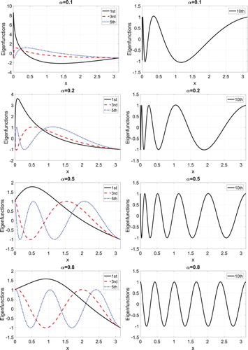The case $\alpha =1$ leads to an exact quadratic growth. To visually get more sense of how the eigensolutions look like, in Figure 2 we plot the eigenfunctions of this example, $\varphi (x,\lambda )$ of different orders and corresponding to different values of α used in Figure 1. We realize that, for α values very close to 0, e.g. $\alpha =0.1$, most of the roots of the eigenfunctions are accumulated on a around of zero and have minimal values and so close to 0. Also, for α values sufficiently away from 0, especially as α approaches 1, e.g. $\alpha =0.8$, the roots (the nodal points) are distributed in the interval $[0,\pi ]$. We can see that the conditions of oscillation theorem 5.2 are provided.

Figure 1. Growth of the eigenvalues of CFSLP in Example 5.1, versus n, corresponding to different fractional-order $\alpha =0.1$; (a): sublinear growth, $\alpha =0.2$ and 0.5; (a): superlinear-subquadratic growth, and $\alpha =0.6$; (b): subquadratic growth, $\alpha =0.8$; (b): quadratic growth. Here we compare the growth of the eigenvalues to the classical case, i.e. $\alpha =1.0$ with quadratic growth. The blue line denotes the linear growth. (a) The first ten eigenvalues for $\alpha =0.1,0.2,0.5$. (b) The first ten eigenvalues for $\alpha =0.6,0.8,1.0$.

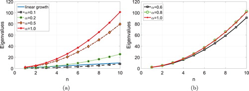
Figure 2. Eigenfunctions of CFSLP in Example 5.1, versus x, corresponding to the fractional order $\alpha =0.1$ (first row), $\alpha =0.2$ (second row), $\alpha =0.5$ (third row), and $\alpha =0.8$ (last row), for $n=1,3,5$ (left column), $n=10$ (right column).

The nodal points of the Equation (1(1) ${\ell }_{\alpha }y:=-D_x^{\alpha }{D}_x^{\alpha }y+q\left(x\right)y=\lambda y,0<x<\pi ,$(1) )–(2(2) $U\left(y\right):=D_x^{\alpha }y\left(0\right)-hy\left(0\right)=0,V\left(y\right):=D_x^{\alpha }y\left(\pi \right)+Hy\left(\pi \right)=0,$(2) ) with $h=H=1$ obtained from the relation (51(9) $\begin{array}{rl}{y}_n^j& =\left(j-\frac{1}{2}\right)\frac{\pi }{{\rho }_n}+\frac{1}{{\rho }_n^2}\left(h+\frac{1}{2}{\int }_0^{y_n^j}\left(1+\cos \left(2{\rho }_{n}t\right)\right)q\left((\alpha t{)}^{\frac{1}{\alpha }}\right)t^{1-\alpha }{\mathrm{d}}_{\alpha }t\right)+o\left(\frac{1}{{\rho }_n^3}\right),\end{array}$(9) ), are given as (67) $x_n^j={\left(\alpha y_n^j\right)}^{\frac{1}{\alpha }},\mathrm{\forall }n>1,j=\overline{1,n},$(67) where $y_n^j=\frac{{\pi }^{\alpha }}{\alpha }\left(\frac{j-1/2}{n}\right)+\frac{{\pi }^{\alpha -1}}{\alpha n^2}\left\{\frac{{\pi }^{\alpha -1}}{\alpha }+\frac{{\pi }^{2\alpha -2}{n}^2}{4{\alpha }^2(n^2-1)}\sin \left(\frac{2\pi (j-1/2)}{n}\right)\right\}+o\left(\frac{1}{n^3}\right).$ We calculate in Table 1 the numerical results of true nodal points and their predictions by the asymptotic formula (67(67) $x_n^j={\left(\alpha y_n^j\right)}^{\frac{1}{\alpha }},\mathrm{\forall }n>1,j=\overline{1,n},$(67) ). The true nodal points are calculated by Newton's method, and the values are precise in the first eight digits (which is set to $1.0\times {10}^{-12}$ in our computation). We observe that, as α values away from 0, the asymptotic formula (67(67) $x_n^j={\left(\alpha y_n^j\right)}^{\frac{1}{\alpha }},\mathrm{\forall }n>1,j=\overline{1,n},$(67) ) is a good approximation not only for sufficiently large n but also for small spectral numbers, especially for α values close to 1. This is in stark coincidence with the classical case $\alpha =1$, where the asymptotic formula is very accurate even for relatively small n, (See Figure 2 and Table 1). Also, we obtain the absolute errors, $e_n^j$, between the true (${\mathrm{\Lambda }}_n^j$, the roots of Equation (66(33) $\begin{array}{rl}\varphi (x,\lambda )& =\cos \left(\frac{n{x}^{\alpha }}{{\pi }^{\alpha -1}}\right)+\frac{{\pi }^{\alpha -1}}{\alpha n}\left(1+\frac{{\pi }^{\alpha -1}}{4\alpha }\sin \left(\frac{2x^{\alpha }}{{\pi }^{\alpha -1}}\right)\right)\sin \left(\frac{n{x}^{\alpha }}{{\pi }^{\alpha -1}}\right)\\ & -\frac{{\pi }^{3\alpha -3}}{4{\alpha }^3{n}^2}\left(1+\frac{{\pi }^{\alpha -1}}{8\alpha }\sin \left(\frac{2x^{\alpha }}{{\pi }^{\alpha -1}}\right)\right)\sin \left(\frac{2x^{\alpha }}{{\pi }^{\alpha -1}}\right)\cos \left(\frac{n{x}^{\alpha }}{{\pi }^{\alpha -1}}\right)\\ & +\frac{{\pi }^{2\alpha -2}}{8{\alpha }^{2}n}\left[\frac{1}{n+1}\cos \left(\frac{2(n+1)x^{\alpha }}{{\pi }^{\alpha -1}}\right)\right.\\ & +\left.\frac{1}{n-1}\cos \left(\frac{2(n-1)x^{\alpha }}{{\pi }^{\alpha -1}}\right)-\frac{2n}{n^2-1}\right]\cos \left(\frac{n{x}^{\alpha }}{{\pi }^{\alpha -1}}\right)\\ & +\frac{{\pi }^{2\alpha -2}}{8{\alpha }^{2}n}\left[\frac{1}{n+1}\sin \left(\frac{2(n+1)x^{\alpha }}{{\pi }^{\alpha -1}}\right)+\frac{1}{n-1}\sin \left(\frac{2(n-1)x^{\alpha }}{{\pi }^{\alpha -1}}\right)\right]\\ & \times \sin \left(\frac{n{x}^{\alpha }}{{\pi }^{\alpha -1}}\right)+o\left(\frac{1}{n^2}\right).\end{array}$(33) ) obtained by Newton's method) and explicit nodal points $x_n^j$, for n=2,5 and n=10, $j=\overline{1,n}$, corresponding to the fractional-order $\alpha =0.1,0.5,0.8$, and $\alpha =1.0$ which are seen in Table 1.

Table 1. Numerical values of nodal points and absolute errors between the true and predicted values, for $n=2$ (Part I), $n=5$ (Part II), $n=10$ (Part III), corresponding to the fractional order $\alpha =0.1,0.5,0.8$ and $\alpha =1.0$ in Example 5.1.

Part I
	$\alpha =0.1$			$\alpha =0.5$
j	$x_2^j$	${\mathrm{\Lambda }}_2^j$	$e_2^j=|{\mathrm{\Lambda }}_2^j-x_2^j|$	$x_2^j$	${\mathrm{\Lambda }}_2^j$	$e_2^j=|{\mathrm{\Lambda }}_2^j-x_2^j|$
$j=1$	0.79795646	0.00755340	0.79040306	0.43841717	0.43374141	0.00467576
$j=2$	0.08393900	0.10923447	0.02529547	2.04099213	2.03833149	0.00266064
	$\alpha =0.8$			$\alpha =1.0$
j	$x_2^j$	${\mathrm{\Lambda }}_2^j$	$e_2^j=|{\mathrm{\Lambda }}_2^j-x_2^j|$	$x_2^j$	${\mathrm{\Lambda }}_2^j$	$e_2^j=|{\mathrm{\Lambda }}_2^j-x_2^j|$
$j=1$	0.86188668	0.85947272	0.00241396	1.11873150	1.11611607	0.00261543
$j=2$	2.38767308	2.38640428	0.00126881	2.52286116	2.52176727	0.00109390
Part II
	$\alpha =0.1$			$\alpha =0.5$
j	$x_5^j$	${\mathrm{\Lambda }}_5^j$	$e_5^j=|{\mathrm{\Lambda }}_5^j-x_5^j|$	$x_5^j$	${\mathrm{\Lambda }}_5^j$	$e_5^j=|{\mathrm{\Lambda }}_5^j-x_5^j|$
$j=1$	0.00000006	0.00000014	0.00000008	0.04289391	0.04302355	0.00012963
$j=2$	0.00022840	0.00020056	0.00002784	0.31845425	0.31831932	0.00013493
$j=3$	0.00732235	0.00633326	0.00098909	0.83118179	0.83037995	0.00080184
$j=4$	0.09565772	0.09467769	0.00098003	1.58524700	1.58472080	0.00052620
$j=5$	1.37384635	1.38195607	0.00810973	2.61234481	2.61269041	0.00034560
	$\alpha =0.8$			$\alpha =1.0$
j	$x_5^j$	${\mathrm{\Lambda }}_5^j$	$e_5^j=|{\mathrm{\Lambda }}_5^j-x_5^j|$	$x_5^j$	${\mathrm{\Lambda }}_5^j$	$e_5^j=|{\mathrm{\Lambda }}_5^j-x_5^j|$
$j=1$	0.20944039	0.20969811	0.00025772	0.36028203	0.36064364	0.00036161
$j=2$	0.74365827	0.74350999	0.00014828	0.99238463	0.99222420	0.00016044
$j=3$	1.36281003	1.36224788	0.00056214	1.61079633	1.61025542	0.00054090
$j=4$	2.04584277	2.04554800	0.00029477	2.22920802	2.22894669	0.00026133
$j=5$	2.79504166	2.79520949	0.00016783	2.86131063	2.86145012	0.00013949
Part III
	$\alpha =0.1$			$\alpha =0.5$
j	$x_{10}^j$	${\mathrm{\Lambda }}_{10}^j$	$e_{10}^j=|{\mathrm{\Lambda }}_{10}^j-x_{10}^j|$	$x_{10}^j$	${\mathrm{\Lambda }}_{10}^j$	$e_{10}^j=|{\mathrm{\Lambda }}_{10}^j-x_{10}^j|$
$j=1$	3.9305E-12	4.2962E-12	3.6574E-13	0.00912970	0.00913295	0.00000325
$j=2$	6.2024E-08	6.5732E-08	3.7074E-09	0.07491270	0.07492104	0.00000835
$j=3$	0.00000686	0.00000704	0.00000018	0.20366598	0.20366814	0.00000216
$j=4$	0.00014962	0.00014951	0.00000012	0.39462596	0.39460721	0.00001875
$j=5$	0.00146975	0.00145455	0.00001520	0.64727012	0.64722841	0.00004170
$j=6$	0.00922620	0.00915910	0.00006710	0.96168473	0.96163414	0.00005059
$j=7$	0.04433974	0.04424282	0.00009693	1.33863427	1.33859167	0.00004260
$j=8$	0.17957701	0.17949595	0.00008106	1.77926940	1.77924472	0.00002468
$j=9$	0.64125647	0.64101566	0.00024082	2.28458511	2.28458564	0.00000053
$j=10$	2.04973048	2.05201236	0.00228188	2.85487250	2.85490624	0.00003374
	$\alpha =0.8$			$\alpha =1.0$
j	$x_{10}^j$	${\mathrm{\Lambda }}_{10}^j$	$e_{10}^j=|{\mathrm{\Lambda }}_{10}^j-x_{10}^j|$	$x_{10}^j$	${\mathrm{\Lambda }}_{10}^j$	$e_{10}^j=|{\mathrm{\Lambda }}_{10}^j-x_{10}^j|$
$j=1$	0.08066409	0.08067607	0.00001199	0.16785998	0.16788030	0.00002033
$j=2$	0.30260192	0.30261503	0.00001310	0.48328187	0.48329898	0.00001711
$j=3$	0.56637602	0.56637707	0.00000105	0.79792342	0.79792469	0.00000127
$j=4$	0.85725225	0.85723408	0.00001817	1.11160040	1.11158126	0.00001914
$j=5$	1.16886402	1.16883177	0.00003225	1.42449704	1.42446505	0.00003199
$j=6$	1.49787964	1.49784586	0.00003378	1.73709561	1.73706372	0.00003189
$j=7$	1.84244158	1.84241622	0.00002537	2.04999225	2.04996929	0.00002297
$j=8$	2.20135110	2.20133810	0.00001299	2.36366924	2.36365788	0.00001136
$j=9$	2.57354517	2.57354607	0.00000090	2.67831078	2.67831152	0.00000074
$j=10$	2.95780777	2.95782316	0.00001540	2.99373267	2.99374535	0.00001267

Example 5.2

Let $\left\{y_n^j\right\}\subset Y_0$ be the dense subset of nodal points in $(0,{\pi }^{\alpha }/\alpha )$ given by the following asmptotics: (86) $\begin{array}{rl}{y}_n^j& =\frac{{\pi }^{\alpha }}{\alpha }\left(\frac{j-1/2}{n}\right)+\frac{{\pi }^{\alpha -1}}{\alpha n^2}\left\{-\frac{{\pi }^{\alpha -1}}{\alpha }\left(\frac{j-1/2}{n}\right){\omega }_{\alpha }+\frac{{\pi }^{\alpha -1}}{2\alpha }\left[\frac{{\pi }^{2\alpha -2}}{\alpha ({\pi }^{2\alpha -2}+4)}\right.\right.\\ & \times \left\{\exp \left({\pi }^{\alpha }\left(\frac{j-1/2}{n}\right)\right)\left(\frac{2}{{\pi }^{\alpha -1}}\sin \left(\frac{2\pi (j-1/2)}{n}\right)\right.\right.\\ & \left.\left.+\left.\left.\cos \left(\frac{2\pi (j-1/2)}{n}\right)\right)-1\right\}\right]\right\}+o\left(\frac{1}{n^3}\right),j=\overline{1,n},\end{array}$(86) where ${\omega }_{\alpha }=1+\frac{{\pi }^{2\alpha -2}}{2\alpha ({\pi }^{2\alpha -2}+4)}(\exp ({\pi }^{\alpha })-1)$. From (68(86) $\begin{array}{rl}{y}_n^j& =\frac{{\pi }^{\alpha }}{\alpha }\left(\frac{j-1/2}{n}\right)+\frac{{\pi }^{\alpha -1}}{\alpha n^2}\left\{-\frac{{\pi }^{\alpha -1}}{\alpha }\left(\frac{j-1/2}{n}\right){\omega }_{\alpha }+\frac{{\pi }^{\alpha -1}}{2\alpha }\left[\frac{{\pi }^{2\alpha -2}}{\alpha ({\pi }^{2\alpha -2}+4)}\right.\right.\\ & \times \left\{\exp \left({\pi }^{\alpha }\left(\frac{j-1/2}{n}\right)\right)\left(\frac{2}{{\pi }^{\alpha -1}}\sin \left(\frac{2\pi (j-1/2)}{n}\right)\right.\right.\\ & \left.\left.+\left.\left.\cos \left(\frac{2\pi (j-1/2)}{n}\right)\right)-1\right\}\right]\right\}+o\left(\frac{1}{n^3}\right),j=\overline{1,n},\end{array}$(86) ), we deduce (87) $\begin{array}{rl}{l}_n^j& =\frac{{\pi }^{\alpha }}{\alpha n}+\frac{{\pi }^{\alpha -1}}{\alpha n^2}\left\{-\frac{{\pi }^{\alpha -1}}{\alpha n}{\omega }_{\alpha }+\frac{{\pi }^{\alpha -1}}{2\alpha }\left[\frac{{\pi }^{2\alpha -2}}{\alpha ({\pi }^{2\alpha -2}+4)}\left\{\exp \left({\pi }^{\alpha }\left(\frac{j+1/2}{n}\right)\right)\right.\right.\right.\\ & \times \left(\frac{2}{{\pi }^{\alpha -1}}\sin \left(\frac{2\pi (j+1/2)}{n}\right)+\cos \left(\frac{2\pi (j+1/2)}{n}\right)\right)-\exp \left({\pi }^{\alpha }\left(\frac{j-1/2}{n}\right)\right)\\ & \left.\left.\left.\times \left(\frac{2}{{\pi }^{\alpha -1}}\sin \left(\frac{2\pi (j-1/2)}{n}\right)+\cos \left(\frac{2\pi (j-1/2)}{n}\right)\right)\right\}\right]\right\}+o\left(\frac{1}{n^3}\right),j=\overline{1,n}.\end{array}$(87) Therefore, using (54(54) $\underset{n\to \mathrm{\infty }}{lim}\frac{\alpha n^2}{{\pi }^{\alpha -1}}\left[y_n^j-{\gamma }_n^j\right]\stackrel{\mathrm{d}\mathrm{e}\mathrm{f}}{=}f\left(x\right),$(54) ) and (55(55) $f\left(x\right)=\frac{{\pi }^{\alpha -1}}{\alpha }\left(h+\frac{1}{2}{\int }_0^{x}q\left(t\right){\mathrm{d}}_{\alpha }t\right)-\frac{x^{\alpha }}{\alpha }\left(\frac{{\omega }_{\alpha }}{\pi }\right).$(55) ), and Algorithm 5.1, we get $\begin{array}{rl}f\left(x\right)& =-\frac{{\omega }_{\alpha }}{\pi }\left(\frac{x^{\alpha }}{\alpha }\right)+\frac{{\pi }^{3\alpha -3}}{2{\alpha }^2({\pi }^{2\alpha -2}+4)}\\ & \times \left\{\exp \left(x^{\alpha }\right)\left(\frac{2}{{\pi }^{\alpha -1}}\sin \left(\frac{2x^{\alpha }}{{\pi }^{\alpha -1}}\right)+\cos \left(\frac{2x^{\alpha }}{{\pi }^{\alpha -1}}\right)\right)-1\right\}.\end{array}$ By virtue of (57(70) $\begin{array}{rl}& q\left(x\right)-⟨q⟩=\frac{2{\alpha }^2}{{\pi }^{2\alpha -2}}\left[\frac{f\left(0\right)-f\left(\pi \right)}{\pi }\right]+\frac{2\alpha }{{\pi }^{\alpha -1}}{D}_x^{\alpha }f\left(x\right),\end{array}$(70) )–(58(71) $\begin{array}{rl}& h=\frac{\alpha }{{\pi }^{\alpha -1}}f\left(0\right),H=-\frac{\alpha }{{\pi }^{\alpha -1}}f\left(\pi \right),\end{array}$(71) ), we compute $q\left(x\right)=\exp \left(x^{\alpha }\right)\cos \left(\frac{2x^{\alpha }}{{\pi }^{\alpha -1}}\right)$, $h=0$, $H=1$. Another method for calculating the potential function $q\left(x\right)$ is using Algorithm 5.2. Theorem 5.9 with (69(87) $\begin{array}{rl}{l}_n^j& =\frac{{\pi }^{\alpha }}{\alpha n}+\frac{{\pi }^{\alpha -1}}{\alpha n^2}\left\{-\frac{{\pi }^{\alpha -1}}{\alpha n}{\omega }_{\alpha }+\frac{{\pi }^{\alpha -1}}{2\alpha }\left[\frac{{\pi }^{2\alpha -2}}{\alpha ({\pi }^{2\alpha -2}+4)}\left\{\exp \left({\pi }^{\alpha }\left(\frac{j+1/2}{n}\right)\right)\right.\right.\right.\\ & \times \left(\frac{2}{{\pi }^{\alpha -1}}\sin \left(\frac{2\pi (j+1/2)}{n}\right)+\cos \left(\frac{2\pi (j+1/2)}{n}\right)\right)-\exp \left({\pi }^{\alpha }\left(\frac{j-1/2}{n}\right)\right)\\ & \left.\left.\left.\times \left(\frac{2}{{\pi }^{\alpha -1}}\sin \left(\frac{2\pi (j-1/2)}{n}\right)+\cos \left(\frac{2\pi (j-1/2)}{n}\right)\right)\right\}\right]\right\}+o\left(\frac{1}{n^3}\right),j=\overline{1,n}.\end{array}$(87) ) imply $\underset{n\to \mathrm{\infty }}{lim}\frac{2{\alpha }^2{n}^2}{{\pi }^{2\alpha -2}}[\frac{\alpha n}{{\pi }^{\alpha }}{l}_n^j-1]=\exp \left(x^{\alpha }\right)\cos \left(\frac{2x^{\alpha }}{{\pi }^{\alpha -1}}\right)-⟨q⟩-\frac{2\alpha }{{\pi }^{\alpha }}$, which concludes $q\left(x\right)=\exp \left(x^{\alpha }\right)\cos \left(\frac{2x^{\alpha }}{{\pi }^{\alpha -1}}\right)$, and using (68(86) $\begin{array}{rl}{y}_n^j& =\frac{{\pi }^{\alpha }}{\alpha }\left(\frac{j-1/2}{n}\right)+\frac{{\pi }^{\alpha -1}}{\alpha n^2}\left\{-\frac{{\pi }^{\alpha -1}}{\alpha }\left(\frac{j-1/2}{n}\right){\omega }_{\alpha }+\frac{{\pi }^{\alpha -1}}{2\alpha }\left[\frac{{\pi }^{2\alpha -2}}{\alpha ({\pi }^{2\alpha -2}+4)}\right.\right.\\ & \times \left\{\exp \left({\pi }^{\alpha }\left(\frac{j-1/2}{n}\right)\right)\left(\frac{2}{{\pi }^{\alpha -1}}\sin \left(\frac{2\pi (j-1/2)}{n}\right)\right.\right.\\ & \left.\left.+\left.\left.\cos \left(\frac{2\pi (j-1/2)}{n}\right)\right)-1\right\}\right]\right\}+o\left(\frac{1}{n^3}\right),j=\overline{1,n},\end{array}$(86) ) and Corollary 5.11, we obtain $h=0,H=1$.

6. Concluding remarks

We expanded the spectral theory for CFSL operator ${\ell }_{\alpha }$, and proved that the eigenvalues are all real, simple and the eigenfunctions corresponding to distinct eigenvalues are orthogonal in the $L_{\alpha }^2(0,\pi )$-space. Also, we presented asymptotic formulae for the eigenvalues and eigenfunctions, and then, we showed that every nontrivial solution u of (1(1) ${\ell }_{\alpha }y:=-D_x^{\alpha }{D}_x^{\alpha }y+q\left(x\right)y=\lambda y,0<x<\pi ,$(1) ) and its CF-derivative $D_x^{\alpha }u$ in $[0,\pi ]$ are entire functions of λ of order 1/2, and consequently by Hadamard's factorization theorem we obtain the infinite product representation for the characteristic function $\mathrm{\Delta }\left(\lambda \right)$ of $L_{\alpha }$. Next, we indicated that the obtained eigenfunctions are complete in different Hilbert space, and provided sufficient conditions under which the Fourier series for the eigenfunctions converges uniformly on $[0,\pi ]$. Moreover, we have presented a first analytical study of the theory of regularized traces and inverse nodal problems for CFSL operator ${\ell }_{\alpha }$. The experimental and numerical observations lead to some interesting conjectures for the CFSLP:

1. Thanks to the asymptotic formula (40(40) ${\lambda }_n={\rho }_n^2=\left(\frac{{\alpha }^2}{{\pi }^{2\alpha -2}}\right)n^2+\frac{2\alpha {\omega }_{\alpha }}{{\pi }^{\alpha }}+O\left(\frac{1}{n^2}\right),$(40) ) of the eigenvalues, there are several modes of growth referred to as a sublinear mode corresponding to $\alpha \to 0$, a quadratic mode which corresponds to $\alpha \to 1$, and a superlinear-subquadratic mode corresponding to other values α of $(0,1)$.

2. The presented nodal points $x_n^1,x_n^2,\dots ,x_n^n$ set up the increasing sequence. On the other hand, one can observe that the nodal points decrease with decreasing the order of derivative α. Also, for sufficiently large n, numerical example confirm the validity of the oscillation theorem for this type of the FSLP. Therefore, only the location of the zeros of eigenfunctions depends on the conformable derivative order, i.e. when the fractional-order α sufficiently away from 0 and approaches 1, similar to the classic case, the distribution of the zeros of the eigenfunctions in the interval $(a,b)$ is uniform.

3. For each $\alpha \in (0,1]$, any dense subset of the elements constructed by of nodal points, and the length of those elements completely determines the potential q and the coefficients of the boundary conditions in the CFSLP (1(1) ${\ell }_{\alpha }y:=-D_x^{\alpha }{D}_x^{\alpha }y+q\left(x\right)y=\lambda y,0<x<\pi ,$(1) )–(2(2) $U\left(y\right):=D_x^{\alpha }y\left(0\right)-hy\left(0\right)=0,V\left(y\right):=D_x^{\alpha }y\left(\pi \right)+Hy\left(\pi \right)=0,$(2) ). Also, by increasing the order of derivative α, the asymptotic formulas obtained for the nodal points are in good agreement with the exact ones.

The authors believe that the new conceptions of the theory of CFSLPs not only can be applied to solve other problems with CF derivatives such as CF partial differential equations, CF integro-differential equations, CF partial integro-differential equations and CF optimal control problems and so on but can be easily used to solve the mentioned problems with integer order derivatives. Apart from these theoretical aspects, the rigorous analysis of appropriate numerical schemes is also of immense interest. In particular, the error estimates for the eigenvalue approximations, the rate of convergence for numerical schemes, numerical solution of inverse nodal problems, etc.

Disclosure statement

No potential conflict of interest was reported by the authors.

Appendix

A.1. Proof of Theorem 3.3

The functions ${\varphi }_1(x,\lambda )=\cos \left(\frac{\rho }{\alpha }{x}^{\alpha }\right)$ and ${\varphi }_2(x,\lambda )={\rho }^{-1}\sin \left(\frac{\rho }{\alpha }{x}^{\alpha }\right)$ are the solutions of $D_x^{\alpha }{D}_x^{\alpha }y+{\rho }^{2}y=0$ with zero potential and $W_{\alpha }\left[{\varphi }_1\right(\cdot ,\lambda ),{\varphi }_1(\cdot ,\lambda \left)\right]=1$, where $\rho :=\sqrt{\lambda }$ is defined with respect to the principal branch. For all $x\in [0,\pi ]$, $\lambda \in \mathbb{C}$, we define the sequence $\left\{y_n\right(\cdot ,\lambda ){\}}_{n=1}^{\mathrm{\infty }}$ of successive approximations by (A1) $y_{n+1}(x,\lambda )=y_1(x,\lambda )+{\int }_0^x\left\{{\varphi }_2\right(x,\lambda \left){\varphi }_1\right(t,\lambda )-{\varphi }_1(x,\lambda \left){\varphi }_2\right(t,\lambda \left)\right\}q\left(t\right)y_n(t,\lambda ){\mathrm{d}}_{\alpha }t,$(A1) where $y_1(x,\lambda )=c_1{\varphi }_1(x,\lambda )+c_2{\varphi }_2(x,\lambda )$. We prove that for each fixed $\lambda \in \mathbb{C}$ the uniform limit of $y_n(\cdot ,\lambda )$ as $n\to \mathrm{\infty }$ exists and defines a solution of (1(1) ${\ell }_{\alpha }y:=-D_x^{\alpha }{D}_x^{\alpha }y+q\left(x\right)y=\lambda y,0<x<\pi ,$(1) ) and (10(10) $\varphi (0,\lambda )=c_1,D_x^{\alpha }\varphi (0,\lambda )=c_2,(\lambda \in \mathbb{C}).$(10) ). Let $\lambda \in \mathbb{C}$ be fixed. There exist positive numbers $K\left(\lambda \right)$ and $\tilde{K}\left(\lambda \right)$ such that $|{\varphi }_i(x,\lambda )|\le \sqrt{K\left(\lambda \right)/2}$ for $i=1,2$ and $|y_1(x,\lambda )|\le \tilde{K}\left(\lambda \right)$, where $\tilde{K}\left(\lambda \right):=(|c_1|+|c_2|)\sqrt{K\left(\lambda \right)/2}$, for all $x\in [0,\pi ]$. Let us show by induction that (A2) $|y_{n+1}(x,\lambda )-y_n(x,\lambda )|\le \tilde{K}\left(\lambda \right)\frac{{\left(K\left(\lambda \right)Q_0\left(x\right)\right)}^n}{n!},x\in [0,\pi ],n\in \mathbb{N},$(A2) where $Q_0\left(x\right)={\int }_0^x|q\left(t\right)|{\mathrm{d}}_{\alpha }t$. Indeed, for $n=1$, (A2(A2) $|y_{n+1}(x,\lambda )-y_n(x,\lambda )|\le \tilde{K}\left(\lambda \right)\frac{{\left(K\left(\lambda \right)Q_0\left(x\right)\right)}^n}{n!},x\in [0,\pi ],n\in \mathbb{N},$(A2) ) is obvious. Suppose that (A2(A2) $|y_{n+1}(x,\lambda )-y_n(x,\lambda )|\le \tilde{K}\left(\lambda \right)\frac{{\left(K\left(\lambda \right)Q_0\left(x\right)\right)}^n}{n!},x\in [0,\pi ],n\in \mathbb{N},$(A2) ) is valid for a certain fixed $n\ge 1$. From (A1(A1) $y_{n+1}(x,\lambda )=y_1(x,\lambda )+{\int }_0^x\left\{{\varphi }_2\right(x,\lambda \left){\varphi }_1\right(t,\lambda )-{\varphi }_1(x,\lambda \left){\varphi }_2\right(t,\lambda \left)\right\}q\left(t\right)y_n(t,\lambda ){\mathrm{d}}_{\alpha }t,$(A1) ), we get (A3) $|y_{n+2}(x,\lambda )-y_{n+1}(x,\lambda )|\le K\left(\lambda \right){\int }_0^x|q\left(t\right)||y_{n+1}(t,\lambda )-y_n(t,\lambda )|{\mathrm{d}}_{\alpha }t.$(A3) Substituting (A2(A2) $|y_{n+1}(x,\lambda )-y_n(x,\lambda )|\le \tilde{K}\left(\lambda \right)\frac{{\left(K\left(\lambda \right)Q_0\left(x\right)\right)}^n}{n!},x\in [0,\pi ],n\in \mathbb{N},$(A2) ) into the right-hand side of (A3(A3) $|y_{n+2}(x,\lambda )-y_{n+1}(x,\lambda )|\le K\left(\lambda \right){\int }_0^x|q\left(t\right)||y_{n+1}(t,\lambda )-y_n(t,\lambda )|{\mathrm{d}}_{\alpha }t.$(A3) ), we calculate $\begin{array}{rl}|y_{n+2}(x,\lambda )-y_{n+1}(x,\lambda )|& \le \tilde{K}\left(\lambda \right)\frac{\left(K\right(\lambda ){)}^{n+1}}{n!}{\int }_0^x|q\left(t\right)|\left(Q_0\right(t){)}^n{\mathrm{d}}_{\alpha }t\\ & =\tilde{K}\left(\lambda \right)\frac{\left(K\right(\lambda ){)}^{n+1}}{n!}{\int }_0^x\left(Q_0\right(t\left){)}^n{D}_t^{\alpha }{Q}_0\right(t){\mathrm{d}}_{\alpha }t=\tilde{K}(\lambda )\frac{{\left(K\left(\lambda \right)Q_0\left(x\right)\right)}^{n+1}}{(n+1)!}.\end{array}$ It follows from [49, Theorem 26] and $q\left(x\right)\in L_{\alpha }^2(0,\pi )$ that $\parallel q{\parallel }_{1,\alpha }\le \sqrt{{\alpha }^{-1}{\pi }^{\alpha }}\parallel q{\parallel }_{2,\alpha }<\mathrm{\infty }.$ Consequently by Weierstrass M-test the series (A4) $y(x,\lambda )=y_1(x,\lambda )+\sum _{n=1}^{\mathrm{\infty }}\left\{y_{n+1}(x,\lambda )-y_n(x,\lambda )\right\}.$(A4) Since the n-th partial sums of the series is nothing but $y_{n+1}(\cdot ,\lambda )$, then $y_{n+1}(\cdot ,\lambda )$ approaches a function $\varphi (\cdot ,\lambda )$ uniformly on $[0,\pi ]$ as $n\to \mathrm{\infty }$, where $\varphi (\cdot ,\lambda )$ is the sum of the series. Similarly, we can also prove by induction on n that $D_x^{\alpha }{y}_{n+1}(\cdot ,\lambda )$ approaches a function $D_x^{\alpha }\varphi (\cdot ,\lambda )$ uniformly on $[0,\pi ]$ as $n\to \mathrm{\infty }$. Hence, both $\varphi (\cdot ,\lambda )$ and $D_x^{\alpha }\varphi (\cdot ,\lambda )$ are continuous, i.e. $\varphi (\cdot ,\lambda )\in C_{\alpha }^2[0,\pi ]$. Because of the uniform convergence, letting $n\to \mathrm{\infty }$ in (A1(A1) $y_{n+1}(x,\lambda )=y_1(x,\lambda )+{\int }_0^x\left\{{\varphi }_2\right(x,\lambda \left){\varphi }_1\right(t,\lambda )-{\varphi }_1(x,\lambda \left){\varphi }_2\right(t,\lambda \left)\right\}q\left(t\right)y_n(t,\lambda ){\mathrm{d}}_{\alpha }t,$(A1) ), we obtain $\begin{array}{rl}\varphi (x,\lambda )& =c_1{\varphi }_1(x,\lambda )+c_2{\varphi }_2(x,\lambda )+{\int }_0^x\left\{{\varphi }_2\right(x,\lambda \left){\varphi }_1\right(t,\lambda )-{\varphi }_1(x,\lambda \left){\varphi }_2\right(t,\lambda \left)\right\}q\left(t\right)\varphi (t,\lambda ){\mathrm{d}}_{\alpha }t.\end{array}$ Then, by α-Leibniz rule 2.14, clearly, $\varphi (\cdot ,\lambda )$ satisfies (1(1) ${\ell }_{\alpha }y:=-D_x^{\alpha }{D}_x^{\alpha }y+q\left(x\right)y=\lambda y,0<x<\pi ,$(1) ) and (10(10) $\varphi (0,\lambda )=c_1,D_x^{\alpha }\varphi (0,\lambda )=c_2,(\lambda \in \mathbb{C}).$(10) ). That $\varphi (\cdot ,\lambda )$ is an entire function of the variable λ follows from the uniform convergence of the series (A4(A4) $y(x,\lambda )=y_1(x,\lambda )+\sum _{n=1}^{\mathrm{\infty }}\left\{y_{n+1}(x,\lambda )-y_n(x,\lambda )\right\}.$(A4) ) and the structure of the functions $y_n(\cdot ,\lambda )$. To prove that problem (1(1) ${\ell }_{\alpha }y:=-D_x^{\alpha }{D}_x^{\alpha }y+q\left(x\right)y=\lambda y,0<x<\pi ,$(1) ), (10(10) $\varphi (0,\lambda )=c_1,D_x^{\alpha }\varphi (0,\lambda )=c_2,(\lambda \in \mathbb{C}).$(10) ) has a unique solution, suppose on the contrary that ${\psi }_i(\cdot ,\lambda )$, $i=1,2$, are two solutions of (1(1) ${\ell }_{\alpha }y:=-D_x^{\alpha }{D}_x^{\alpha }y+q\left(x\right)y=\lambda y,0<x<\pi ,$(1) ), (10(10) $\varphi (0,\lambda )=c_1,D_x^{\alpha }\varphi (0,\lambda )=c_2,(\lambda \in \mathbb{C}).$(10) ). Therefore, for $x\in [0,\pi ]$, we can write $\left|{\psi }_1(x,\lambda )-{\psi }_2(x,\lambda )\right|\le {\int }_0^{x}K\left(\lambda \right)|q\left(t\right)\left|{\psi }_1(t,\lambda )-{\psi }_2(t,\lambda )\right|{\mathrm{d}}_{\alpha }t,$ letting $\psi (x,\lambda )=|{\psi }_1(x,\lambda )-{\psi }_2(x,\lambda )|$, we have $\psi (x,\lambda )\le {\int }_0^{x}K\left(\lambda \right)|q\left(t\right)\psi (t,\lambda ){\mathrm{d}}_{\alpha }t$. Thus, the fractional version of Gronwall's inequality (See Lemma 2.15) implies $\psi (x,\lambda )\equiv 0$, and consequently ${\psi }_1(x,\lambda )={\psi }_2(x,\lambda )$ for all $x\in [0,\pi ]$. This completes a proof of the theorem.

A.2. Proof of Theorem 3.12

We denote $G_{\alpha }(x,t,\lambda )=-\frac{1}{\mathrm{\Delta }\left(\lambda \right)}\left\{\begin{array}{cc}\varphi (x,\lambda )\psi (t,\lambda ),& x\le t\\ \varphi (t,\lambda )\psi (x,\lambda ),& x\ge t\end{array}\right.$, and consider the function $\begin{array}{rl}Y(x,\lambda )& ={\int }_0^{\pi }{G}_{\alpha }(x,t,\lambda )f\left(t\right){\mathrm{d}}_{\alpha }t,\\ & =-\frac{1}{\mathrm{\Delta }\left(\lambda \right)}\left(\psi (x,\lambda ){\int }_0^x\varphi (t,\lambda )f\left(t\right){\mathrm{d}}_{\alpha }t+\varphi (x,\lambda ){\int }_x^{\pi }\psi (t,\lambda )f\left(t\right){\mathrm{d}}_{\alpha }t\right).\end{array}$ The function $G_{\alpha }(x,t,\lambda )$ is called Green's function for $L_{\alpha }$. $G_{\alpha }(x,t,\lambda )$ is the kernel of the inverse operator for the CFSL operator, i.e. $Y(x,\lambda )$ is the solution of the boundary value problem ${\ell }_{\alpha }Y-\lambda Y+f\left(x\right)=0,U\left(Y\right)=V\left(Y\right)=0$. From (15(15) $\psi (x,{\lambda }_n)={\beta }_n\varphi (x,{\lambda }_n),{\beta }_n\ne 0.$(15) ), Theorem 3.7 and using Lemma 3.5, we obtain (A5) $Re{s}_{\lambda ={\lambda }_n}Y(x,\lambda )=\frac{1}{{\alpha }_n}\varphi (x,{\lambda }_n){\int }_0^{\pi }f\left(t\right)\varphi (t,{\lambda }_n){\mathrm{d}}_{\alpha }t.$(A5) Let $f\left(x\right)\in L_{\alpha }^2(0,\pi )$ be such that ${\int }_0^{\pi }f\left(t\right)\varphi (t,{\lambda }_n){\mathrm{d}}_{\alpha }t=0,n\ge 0$, then (A5(A5) $Re{s}_{\lambda ={\lambda }_n}Y(x,\lambda )=\frac{1}{{\alpha }_n}\varphi (x,{\lambda }_n){\int }_0^{\pi }f\left(t\right)\varphi (t,{\lambda }_n){\mathrm{d}}_{\alpha }t.$(A5) ) implies that $Re{s}_{\lambda ={\lambda }_n}Y(x,\lambda )=0$, and consequently for each $x\in [0,\pi ]$, the function $Y(x,\lambda )$ is entire in λ. Moreover, it follows from Lemma 3.9 and (30(30) $\begin{array}{rl}& |\mathrm{\Delta }\left(\lambda \right)|\ge C_{\delta }|\rho |\exp \left(\frac{|\tau |}{\alpha }{\pi }^{\alpha }\right),\rho \in G_{\delta },|\rho |\ge {\rho }^{\ast },\end{array}$(30) ) that for a fixed $\delta >0$, and sufficiently large ${\rho }^{\ast }>0$, $|Y(x,\lambda )|\le \frac{C_{\delta }}{|\rho |}$, $\rho \in G_{\delta }$, $|\rho |\ge {\rho }^{\ast }$. Using the maximum principle and Liouville's theorem, we conclude that $Y(x,\lambda )\equiv 0$. Hence,  $f\left(x\right)=0$ a.e. on $(0,\pi )$. Thus (1) is proved. Let now $f\left(x\right)\in AC[0,\pi ]$ be an arbitrary absolutely continuous function. Applying the same arguments as in the proof of [52, Theorem 1.2.1.], we obtain (A6) $Y(x,\lambda )=\frac{f\left(x\right)}{\lambda }-\frac{1}{\lambda }\left(Z_1(x,\lambda )+Z_2(x,\lambda )\right),$(A6) where $\begin{array}{rl}{Z}_1(x,\lambda )& =\frac{1}{\mathrm{\Delta }\left(\lambda \right)}\left(\psi (x,\lambda ){\int }_0^{x}g\left(t\right)D_t^{\alpha }\varphi (t,\lambda ){\mathrm{d}}_{\alpha }t+\varphi (x,\lambda ){\int }_x^{\pi }g\left(t\right)D_t^{\alpha }\psi (t,\lambda ){\mathrm{d}}_{\alpha }t\right),\\ Z_2(x,\lambda )& =\frac{1}{\mathrm{\Delta }\left(\lambda \right)}\left(hf\left(0\right)\psi (x,\lambda )+Hf\left(\pi \right)\varphi (x,\lambda )+\psi (x,\lambda ){\int }_0^{x}q\left(t\right)\varphi (t,\lambda )f\left(t\right){\mathrm{d}}_{\alpha }t\right.\\ & \left.+\varphi (x,\lambda ){\int }_x^{\pi }q\left(t\right)\psi (t,\lambda )f\left(t\right){\mathrm{d}}_{\alpha }t\right),g\left(t\right):=D_t^{\alpha }f\left(t\right).\end{array}$ Using Lemma 3.9 and (30(30) $\begin{array}{rl}& |\mathrm{\Delta }\left(\lambda \right)|\ge C_{\delta }|\rho |\exp \left(\frac{|\tau |}{\alpha }{\pi }^{\alpha }\right),\rho \in G_{\delta },|\rho |\ge {\rho }^{\ast },\end{array}$(30) ), we get for a fixed $\delta >0$, and sufficiently large ${\rho }^{\ast }>0$, (A7) $\underset{0\le x\le \pi }{max}|Z_2(x,\lambda )|\le \frac{C}{|\rho |},\rho \in G_{\delta },|\rho |\ge {\rho }^{\ast }.$(A7) Let now $g\left(t\right)\in L_{\alpha }^1(0,\pi )$. Fix $\epsilon >0$ and choose an absolutely continuous function $g_{\epsilon }\left(t\right)$ such that ${\int }_0^{\pi }|g\left(t\right)-g_{\epsilon }\left(t\right)|{\mathrm{d}}_{\alpha }t<\frac{\epsilon }{2C^{+}}$ (See [49, Definition 16]), where $C^{+}=\underset{0\le x\le \pi }{max}\underset{\begin{array}{c}\rho \in G_{\delta }\end{array}}{sup}\frac{1}{|\mathrm{\Delta }\left(\lambda \right)|}\left(|\psi (x,\lambda )|{\int }_0^x|D_t^{\alpha }\varphi (t,\lambda )|{\mathrm{d}}_{\alpha }t+|\varphi (x,\lambda )|{\int }_x^{\pi }|D_t^{\alpha }\psi (t,\lambda )|{\mathrm{d}}_{\alpha }t\right).$ Then, we have $|Z_1(x,\lambda )|\le |Z_1(x,\lambda ,g_{\epsilon })|+|Z_1(x,\lambda ,g-g_{\epsilon })|\le \epsilon /2+C\left(\epsilon \right)/|\rho |,$ for $\rho \in G_{\delta }$, $|\rho |\ge {\rho }^{\ast }$. Hence (A8) $\begin{array}{r}\underset{\begin{array}{c}|\rho |\to \mathrm{\infty }\\ \rho \in G_{\delta }\end{array}}{lim}\underset{0\le x\le \pi }{max}|Z_1(x,\lambda )|=0.\end{array}$(A8) Consider the contour integral $I_N\left(x\right)=\frac{1}{2\pi i}{\int }_{{\mathrm{\Gamma }}_N}Y(x,\lambda )\mathrm{d}\lambda ,{\mathrm{\Gamma }}_N=\left\{\lambda :|\lambda |={\left(\frac{\alpha }{{\pi }^{\alpha -1}}\right)}^2{\left(N+\frac{1}{2}\right)}^2\right\}.$ It follows from (A6(A6) $Y(x,\lambda )=\frac{f\left(x\right)}{\lambda }-\frac{1}{\lambda }\left(Z_1(x,\lambda )+Z_2(x,\lambda )\right),$(A6) )–(A8(A8) $\begin{array}{r}\underset{\begin{array}{c}|\rho |\to \mathrm{\infty }\\ \rho \in G_{\delta }\end{array}}{lim}\underset{0\le x\le \pi }{max}|Z_1(x,\lambda )|=0.\end{array}$(A8) ) that $I_N\left(x\right)=f\left(x\right)+{\epsilon }_N\left(x\right)$, $\underset{N\to \mathrm{\infty }}{lim}\underset{0\le x\le \pi }{max}|{\epsilon }_N\left(x\right)|=0$. On the other hand, we can calculate $I_N\left(x\right)$ with the help of the residue theorem. From (A5(A5) $Re{s}_{\lambda ={\lambda }_n}Y(x,\lambda )=\frac{1}{{\alpha }_n}\varphi (x,{\lambda }_n){\int }_0^{\pi }f\left(t\right)\varphi (t,{\lambda }_n){\mathrm{d}}_{\alpha }t.$(A5) ), we get $I_N\left(x\right)=\sum _{n=0}^N{c}_n\varphi (x,{\lambda }_n),c_n=\frac{1}{{\alpha }_n}⟨f,\varphi (t,{\lambda }_n)⟩.$ If $N\to \mathrm{\infty }$, we arrive at (34(34) $f\left(x\right)=\sum _{n=0}^{\mathrm{\infty }}{c}_n\varphi (x,{\lambda }_n),c_n=\frac{1}{{\alpha }_n}{\int }_0^{\pi }f\left(t\right)\varphi (t,{\lambda }_n){\mathrm{d}}_{\alpha }t,$(34) ), where the series converges uniformly on $[0,\pi ]$, i.e. (2) is proved. Moreover, by virtue of (1), the Parseval's equality is clear.

A.3. Proof of Lemma 4.1

Let $q\left(x\right)\in W_{\alpha }^2(0,\pi )$. Then, α-integration by parts yields (A9) $\begin{array}{rl}\frac{1}{2}{\int }_0^{x}q\left(t\right)\cos \left(\frac{\rho }{\alpha }(x^{\alpha }-2t^{\alpha })\right){\mathrm{d}}_{\alpha }t& =\frac{1}{4\rho }\sin \left(\frac{\rho }{\alpha }{x}^{\alpha }\right)\left(q\right(x)+q(0\left)\right)\\ & +\frac{1}{4\rho }{\int }_0^x{D}_t^{\alpha }q\left(t\right)\sin \left(\frac{\rho }{\alpha }(x^{\alpha }-2t^{\alpha })\right){\mathrm{d}}_{\alpha }t,\end{array}$(A9) (A10) $\begin{array}{rl}\frac{1}{2\rho }{\int }_0^{x}q\left(t\right)\sin \left(\frac{\rho }{\alpha }(x^{\alpha }-2t^{\alpha })\right){\mathrm{d}}_{\alpha }t& =\frac{1}{4{\rho }^2}\cos \left(\frac{\rho }{\alpha }{x}^{\alpha }\right)\left(q\right(x)-q(0\left)\right)\\ & -\frac{1}{4{\rho }^2}{\int }_0^x{D}_t^{\alpha }q\left(t\right)\cos \left(\frac{\rho }{\alpha }(x^{\alpha }-2t^{\alpha })\right){\mathrm{d}}_{\alpha }t.\end{array}$(A10) It follows from (26(26) $\begin{array}{rl}\varphi (x,\lambda )& =\cos \left(\frac{\rho }{\alpha }{x}^{\alpha }\right)+\frac{q_1\left(x\right)}{\rho }\sin \left(\frac{\rho }{\alpha }{x}^{\alpha }\right)+\frac{1}{2\rho }{\int }_0^{x}q\left(t\right)\sin \left(\frac{\rho }{\alpha }(x^{\alpha }-2t^{\alpha })\right){\mathrm{d}}_{\alpha }t\\ & +O\left(\frac{1}{{\rho }^2}\exp \left(\frac{\left|\tau \right|}{\alpha }{x}^{\alpha }\right)\right),\end{array}$(26) ), (A10(A10) $\begin{array}{rl}\frac{1}{2\rho }{\int }_0^{x}q\left(t\right)\sin \left(\frac{\rho }{\alpha }(x^{\alpha }-2t^{\alpha })\right){\mathrm{d}}_{\alpha }t& =\frac{1}{4{\rho }^2}\cos \left(\frac{\rho }{\alpha }{x}^{\alpha }\right)\left(q\right(x)-q(0\left)\right)\\ & -\frac{1}{4{\rho }^2}{\int }_0^x{D}_t^{\alpha }q\left(t\right)\cos \left(\frac{\rho }{\alpha }(x^{\alpha }-2t^{\alpha })\right){\mathrm{d}}_{\alpha }t.\end{array}$(A10) ) that $\varphi (x,\lambda )=\cos \left(\frac{\rho }{\alpha }{x}^{\alpha }\right)+\frac{q_1\left(x\right)}{\rho }\sin \left(\frac{\rho }{\alpha }{x}^{\alpha }\right)+O\left(\frac{1}{{\rho }^2}\exp \left(\frac{\left|\tau \right|}{\alpha }{x}^{\alpha }\right)\right).$ By putting this asymptotic into the right-hand side of (18(19) $\begin{array}{rl}\varphi (x,\lambda )& =\cos \left(\frac{\rho }{\alpha }{x}^{\alpha }\right)+\frac{h}{\rho }\sin \left(\frac{\rho }{\alpha }{x}^{\alpha }\right)\\ & +\frac{1}{\rho }{\int }_0^x\sin \left(\frac{\rho }{\alpha }(x^{\alpha }-t^{\alpha })\right)q\left(t\right)\varphi (t,\lambda ){\mathrm{d}}_{\alpha }t,\end{array}$(19) ) and from Property 3.2 and (6(6) ${\int }_a^{b}f\left(x\right)D_x^{\alpha }g\left(x\right){\mathrm{d}}_{\alpha }x=fg{|}_a^b-{\int }_a^{b}g\left(x\right)D_x^{\alpha }f\left(x\right){\mathrm{d}}_{\alpha }x.$(6) ), we conclude that (A11) $\begin{array}{rl}\varphi (x,\lambda )& =\cos \left(\frac{\rho }{\alpha }{x}^{\alpha }\right)+\frac{q_1\left(x\right)}{\rho }\sin \left(\frac{\rho }{\alpha }{x}^{\alpha }\right)+\frac{1}{2\rho }{\int }_0^{x}q\left(t\right)\sin \left(\frac{\rho }{\alpha }(x^{\alpha }-2t^{\alpha })\right){\mathrm{d}}_{\alpha }t+I+II,\end{array}$(A11) where (A12) $\begin{array}{rl}I& =-\frac{1}{2{\rho }^2}\cos \left(\frac{\rho }{\alpha }{x}^{\alpha }\right){\int }_0^{x}q\left(t\right)q_1\left(t\right){\mathrm{d}}_{\alpha }t+\frac{1}{2{\rho }^2}{\int }_0^x\cos \left(\frac{\rho }{\alpha }(x^{\alpha }-2t^{\alpha })\right)q\left(t\right)q_1\left(t\right){\mathrm{d}}_{\alpha }t,\\ & =-\frac{1}{2{\rho }^2}\cos \left(\frac{\rho }{\alpha }{x}^{\alpha }\right){\int }_0^{x}q\left(t\right)q_1\left(t\right){\mathrm{d}}_{\alpha }t+\frac{1}{4{\rho }^3}\sin \left(\frac{\rho }{\alpha }{x}^{\alpha }\right)\left(q\left(x\right)q_1\left(x\right)-q\left(0\right)q_1\left(0\right)\right)\\ & +\frac{1}{4{\rho }^3}{\int }_0^x\sin \left(\frac{\rho }{\alpha }(x^{\alpha }-2t^{\alpha })\right)D_t^{\alpha }\left(q\left(t\right)q_1\left(t\right)\right){\mathrm{d}}_{\alpha }t,\\ & =-\frac{1}{2{\rho }^2}\cos \left(\frac{\rho }{\alpha }{x}^{\alpha }\right){\int }_0^{x}q\left(t\right)q_1\left(t\right){\mathrm{d}}_{\alpha }t+O\left(\frac{1}{{\rho }^3}\exp \left(\frac{\left|\tau \right|}{\alpha }{x}^{\alpha }\right)\right).\end{array}$(A12) Since $q\left(x\right)\in L_{\alpha }^2(0,\pi )$, then (A13) $II=O\left(\frac{1}{{\rho }^3}{\int }_0^x\sin \left(\frac{\rho }{\alpha }(x^{\alpha }-t^{\alpha })\right)\exp \left(\frac{\left|\tau \right|}{\alpha }{t}^{\alpha }\right)q\left(t\right){\mathrm{d}}_{\alpha }t\right)=O\left(\frac{1}{{\rho }^3}\exp \left(\frac{\left|\tau \right|}{\alpha }{x}^{\alpha }\right)\right).$(A13) Hence, by substituting (A12(A12) $\begin{array}{rl}I& =-\frac{1}{2{\rho }^2}\cos \left(\frac{\rho }{\alpha }{x}^{\alpha }\right){\int }_0^{x}q\left(t\right)q_1\left(t\right){\mathrm{d}}_{\alpha }t+\frac{1}{2{\rho }^2}{\int }_0^x\cos \left(\frac{\rho }{\alpha }(x^{\alpha }-2t^{\alpha })\right)q\left(t\right)q_1\left(t\right){\mathrm{d}}_{\alpha }t,\\ & =-\frac{1}{2{\rho }^2}\cos \left(\frac{\rho }{\alpha }{x}^{\alpha }\right){\int }_0^{x}q\left(t\right)q_1\left(t\right){\mathrm{d}}_{\alpha }t+\frac{1}{4{\rho }^3}\sin \left(\frac{\rho }{\alpha }{x}^{\alpha }\right)\left(q\left(x\right)q_1\left(x\right)-q\left(0\right)q_1\left(0\right)\right)\\ & +\frac{1}{4{\rho }^3}{\int }_0^x\sin \left(\frac{\rho }{\alpha }(x^{\alpha }-2t^{\alpha })\right)D_t^{\alpha }\left(q\left(t\right)q_1\left(t\right)\right){\mathrm{d}}_{\alpha }t,\\ & =-\frac{1}{2{\rho }^2}\cos \left(\frac{\rho }{\alpha }{x}^{\alpha }\right){\int }_0^{x}q\left(t\right)q_1\left(t\right){\mathrm{d}}_{\alpha }t+O\left(\frac{1}{{\rho }^3}\exp \left(\frac{\left|\tau \right|}{\alpha }{x}^{\alpha }\right)\right).\end{array}$(A12) ), (A13(A13) $II=O\left(\frac{1}{{\rho }^3}{\int }_0^x\sin \left(\frac{\rho }{\alpha }(x^{\alpha }-t^{\alpha })\right)\exp \left(\frac{\left|\tau \right|}{\alpha }{t}^{\alpha }\right)q\left(t\right){\mathrm{d}}_{\alpha }t\right)=O\left(\frac{1}{{\rho }^3}\exp \left(\frac{\left|\tau \right|}{\alpha }{x}^{\alpha }\right)\right).$(A13) ) into (A11(A11) $\begin{array}{rl}\varphi (x,\lambda )& =\cos \left(\frac{\rho }{\alpha }{x}^{\alpha }\right)+\frac{q_1\left(x\right)}{\rho }\sin \left(\frac{\rho }{\alpha }{x}^{\alpha }\right)+\frac{1}{2\rho }{\int }_0^{x}q\left(t\right)\sin \left(\frac{\rho }{\alpha }(x^{\alpha }-2t^{\alpha })\right){\mathrm{d}}_{\alpha }t+I+II,\end{array}$(A11) ), and applying (A10(A10) $\begin{array}{rl}\frac{1}{2\rho }{\int }_0^{x}q\left(t\right)\sin \left(\frac{\rho }{\alpha }(x^{\alpha }-2t^{\alpha })\right){\mathrm{d}}_{\alpha }t& =\frac{1}{4{\rho }^2}\cos \left(\frac{\rho }{\alpha }{x}^{\alpha }\right)\left(q\right(x)-q(0\left)\right)\\ & -\frac{1}{4{\rho }^2}{\int }_0^x{D}_t^{\alpha }q\left(t\right)\cos \left(\frac{\rho }{\alpha }(x^{\alpha }-2t^{\alpha })\right){\mathrm{d}}_{\alpha }t.\end{array}$(A10) ) we arrive at (35(36) $\begin{array}{rl}\varphi (x,\lambda )& =\cos \left(\frac{\rho }{\alpha }{x}^{\alpha }\right)+\frac{q_1\left(x\right)}{\rho }\sin \left(\frac{\rho }{\alpha }{x}^{\alpha }\right)+\frac{q_{20}\left(x\right)}{{\rho }^2}\cos \left(\frac{\rho }{\alpha }{x}^{\alpha }\right)\\ & -\frac{1}{4{\rho }^2}{\int }_0^x{D}_t^{\alpha }q\left(t\right)\cos \left(\frac{\rho }{\alpha }(x^{\alpha }-2t^{\alpha })\right){\mathrm{d}}_{\alpha }t+O\left(\frac{1}{{\rho }^3}\exp \left(\frac{\left|\tau \right|}{\alpha }{x}^{\alpha }\right)\right),\end{array}$(36) ). The formula in (36(37) $\begin{array}{rl}{D}_x^{\alpha }\varphi (x,\lambda )& =-\rho \sin \left(\frac{\rho }{\alpha }{x}^{\alpha }\right)+q_1\left(x\right)\cos \left(\frac{\rho }{\alpha }{x}^{\alpha }\right)+\frac{q_{21}\left(x\right)}{\rho }\sin \left(\frac{\rho }{\alpha }{x}^{\alpha }\right)\\ & +\frac{1}{4\rho }{\int }_0^x{D}_t^{\alpha }q\left(t\right)\sin \left(\frac{\rho }{\alpha }(x^{\alpha }-2t^{\alpha })\right){\mathrm{d}}_{\alpha }t+O\left(\frac{1}{{\rho }^2}\exp \left(\frac{\left|\tau \right|}{\alpha }{x}^{\alpha }\right)\right),\end{array}$(37) ) is proved similarly. Finally, by using (35(36) $\begin{array}{rl}\varphi (x,\lambda )& =\cos \left(\frac{\rho }{\alpha }{x}^{\alpha }\right)+\frac{q_1\left(x\right)}{\rho }\sin \left(\frac{\rho }{\alpha }{x}^{\alpha }\right)+\frac{q_{20}\left(x\right)}{{\rho }^2}\cos \left(\frac{\rho }{\alpha }{x}^{\alpha }\right)\\ & -\frac{1}{4{\rho }^2}{\int }_0^x{D}_t^{\alpha }q\left(t\right)\cos \left(\frac{\rho }{\alpha }(x^{\alpha }-2t^{\alpha })\right){\mathrm{d}}_{\alpha }t+O\left(\frac{1}{{\rho }^3}\exp \left(\frac{\left|\tau \right|}{\alpha }{x}^{\alpha }\right)\right),\end{array}$(36) ), (36(37) $\begin{array}{rl}{D}_x^{\alpha }\varphi (x,\lambda )& =-\rho \sin \left(\frac{\rho }{\alpha }{x}^{\alpha }\right)+q_1\left(x\right)\cos \left(\frac{\rho }{\alpha }{x}^{\alpha }\right)+\frac{q_{21}\left(x\right)}{\rho }\sin \left(\frac{\rho }{\alpha }{x}^{\alpha }\right)\\ & +\frac{1}{4\rho }{\int }_0^x{D}_t^{\alpha }q\left(t\right)\sin \left(\frac{\rho }{\alpha }(x^{\alpha }-2t^{\alpha })\right){\mathrm{d}}_{\alpha }t+O\left(\frac{1}{{\rho }^2}\exp \left(\frac{\left|\tau \right|}{\alpha }{x}^{\alpha }\right)\right),\end{array}$(37) ) and (14(14) $\mathrm{\Delta }\left(\lambda \right)=V\left(\varphi \right)=-U\left(\psi \right).$(14) ), the desired result for $\mathrm{\Delta }\left(\lambda \right)$ can be concluded, i.e. (37(38) $\begin{array}{rl}\mathrm{\Delta }\left(\lambda \right)& =-\rho \sin \left(\frac{\rho }{\alpha }{\pi }^{\alpha }\right)+{\omega }_{\alpha }\cos \left(\frac{\rho }{\alpha }{\pi }^{\alpha }\right)+\frac{{\omega }_0}{\rho }\sin \left(\frac{\rho }{\alpha }{x}^{\alpha }\right)+\frac{k_{{\alpha }_0}\left(\rho \right)}{\rho },\end{array}$(38) ) are valid.

A.4. Proof of Lemma 5.1

For arbitrary $\lambda >0$, let $\rho =\sqrt{\lambda }$. By virtue of Lemma 3.8, the function $\varphi (x,\lambda )$ with the initial conditions $\varphi (0,\lambda )=1$ and $D_x^{\alpha }\varphi (0,\lambda )=h$ is a unique solution of the CF integral equation (18(19) $\begin{array}{rl}\varphi (x,\lambda )& =\cos \left(\frac{\rho }{\alpha }{x}^{\alpha }\right)+\frac{h}{\rho }\sin \left(\frac{\rho }{\alpha }{x}^{\alpha }\right)\\ & +\frac{1}{\rho }{\int }_0^x\sin \left(\frac{\rho }{\alpha }(x^{\alpha }-t^{\alpha })\right)q\left(t\right)\varphi (t,\lambda ){\mathrm{d}}_{\alpha }t,\end{array}$(19) ). Setting $\varphi (t,\lambda )$ in Lemma 3.8 into the right-hand side of (18(19) $\begin{array}{rl}\varphi (x,\lambda )& =\cos \left(\frac{\rho }{\alpha }{x}^{\alpha }\right)+\frac{h}{\rho }\sin \left(\frac{\rho }{\alpha }{x}^{\alpha }\right)\\ & +\frac{1}{\rho }{\int }_0^x\sin \left(\frac{\rho }{\alpha }(x^{\alpha }-t^{\alpha })\right)q\left(t\right)\varphi (t,\lambda ){\mathrm{d}}_{\alpha }t,\end{array}$(19) ), we have $\begin{array}{rl}\varphi (x,\lambda )& =\cos \left(\frac{\rho }{\alpha }{x}^{\alpha }\right)+\frac{h}{\rho }\sin \left(\frac{\rho }{\alpha }{x}^{\alpha }\right)+\frac{1}{\rho }{\int }_0^x\sin \left(\frac{\rho }{\alpha }(x^{\alpha }-t^{\alpha })\right)\cos \left(\frac{\rho }{\alpha }{t}^{\alpha }\right)q\left(t\right){\mathrm{d}}_{\alpha }t\\ & +\frac{1}{{\rho }^2}{\int }_0^x{\int }_0^t\sin \left(\frac{\rho }{\alpha }(x^{\alpha }-t^{\alpha })\right)\sin \left(\frac{\rho }{\alpha }(t^{\alpha }-y^{\alpha })\right)q\left(y\right)q\left(t\right)\varphi (y,\lambda ){\mathrm{d}}_{\alpha }y{\mathrm{d}}_{\alpha }t\\ & +\frac{h}{{\rho }^2}{\int }_0^x\sin \left(\frac{\rho }{\alpha }(x^{\alpha }-t^{\alpha })\right)\sin \left(\frac{\rho }{\alpha }{t}^{\alpha }\right)q\left(t\right){\mathrm{d}}_{\alpha }t.\end{array}$ Thus, by considering $\varphi (x,\lambda )=\cos \left(\frac{\rho }{\alpha }{x}^{\alpha }\right)+O\left({\rho }^{-1}\right)$ and trigonometric calculations, and using (A9(A9) $\begin{array}{rl}\frac{1}{2}{\int }_0^{x}q\left(t\right)\cos \left(\frac{\rho }{\alpha }(x^{\alpha }-2t^{\alpha })\right){\mathrm{d}}_{\alpha }t& =\frac{1}{4\rho }\sin \left(\frac{\rho }{\alpha }{x}^{\alpha }\right)\left(q\right(x)+q(0\left)\right)\\ & +\frac{1}{4\rho }{\int }_0^x{D}_t^{\alpha }q\left(t\right)\sin \left(\frac{\rho }{\alpha }(x^{\alpha }-2t^{\alpha })\right){\mathrm{d}}_{\alpha }t,\end{array}$(A9) ) and (A10(A10) $\begin{array}{rl}\frac{1}{2\rho }{\int }_0^{x}q\left(t\right)\sin \left(\frac{\rho }{\alpha }(x^{\alpha }-2t^{\alpha })\right){\mathrm{d}}_{\alpha }t& =\frac{1}{4{\rho }^2}\cos \left(\frac{\rho }{\alpha }{x}^{\alpha }\right)\left(q\right(x)-q(0\left)\right)\\ & -\frac{1}{4{\rho }^2}{\int }_0^x{D}_t^{\alpha }q\left(t\right)\cos \left(\frac{\rho }{\alpha }(x^{\alpha }-2t^{\alpha })\right){\mathrm{d}}_{\alpha }t.\end{array}$(A10) ), we can write (A14) $\begin{array}{rl}\varphi (x,\lambda )& =\cos \left(\frac{\rho }{\alpha }{x}^{\alpha }\right)+\frac{\sin \left(\frac{\rho }{\alpha }{x}^{\alpha }\right)}{\rho }\left(h+\frac{1}{2}{\int }_0^x\left(1+\cos \left(\frac{2\rho }{\alpha }{t}^{\alpha }\right)\right)q\left(t\right){\mathrm{d}}_{\alpha }t\right)\\ & -\frac{\cos \left(\frac{\rho }{\alpha }{x}^{\alpha }\right)}{2\rho }{\int }_0^x\sin \left(\frac{2\rho }{\alpha }{t}^{\alpha }\right)q\left(t\right){\mathrm{d}}_{\alpha }t-\frac{h\cos \left(\frac{\rho }{\alpha }{x}^{\alpha }\right)}{2{\rho }^2}{\int }_0^{x}q\left(t\right){\mathrm{d}}_{\alpha }t\\ & -\frac{\cos \left(\frac{\rho }{\alpha }{x}^{\alpha }\right)}{4{\rho }^2}{\int }_0^x{\int }_0^{t}q\left(y\right)q\left(t\right){\mathrm{d}}_{\alpha }y{\mathrm{d}}_{\alpha }t+o\left(\frac{1}{{\rho }^2}\right).\end{array}$(A14) If $\varphi (x,\lambda )$ equal to zero and $\sin \left(\frac{\rho }{\alpha }{x}^{\alpha }\right)$ is not close to zero, then by using (A14(A14) $\begin{array}{rl}\varphi (x,\lambda )& =\cos \left(\frac{\rho }{\alpha }{x}^{\alpha }\right)+\frac{\sin \left(\frac{\rho }{\alpha }{x}^{\alpha }\right)}{\rho }\left(h+\frac{1}{2}{\int }_0^x\left(1+\cos \left(\frac{2\rho }{\alpha }{t}^{\alpha }\right)\right)q\left(t\right){\mathrm{d}}_{\alpha }t\right)\\ & -\frac{\cos \left(\frac{\rho }{\alpha }{x}^{\alpha }\right)}{2\rho }{\int }_0^x\sin \left(\frac{2\rho }{\alpha }{t}^{\alpha }\right)q\left(t\right){\mathrm{d}}_{\alpha }t-\frac{h\cos \left(\frac{\rho }{\alpha }{x}^{\alpha }\right)}{2{\rho }^2}{\int }_0^{x}q\left(t\right){\mathrm{d}}_{\alpha }t\\ & -\frac{\cos \left(\frac{\rho }{\alpha }{x}^{\alpha }\right)}{4{\rho }^2}{\int }_0^x{\int }_0^{t}q\left(y\right)q\left(t\right){\mathrm{d}}_{\alpha }y{\mathrm{d}}_{\alpha }t+o\left(\frac{1}{{\rho }^2}\right).\end{array}$(A14) ), we get $\begin{array}{rl}0& =\cot \left(\frac{\rho }{\alpha }{x}^{\alpha }\right)+\frac{1}{\rho }\left(h+\frac{1}{2}{\int }_0^x\left(1+\cos \left(\frac{2\rho }{\alpha }{t}^{\alpha }\right)\right)q\left(t\right){\mathrm{d}}_{\alpha }t\right)\\ & -\frac{\cot \left(\frac{\rho }{\alpha }{x}^{\alpha }\right)}{2\rho }{\int }_0^x\sin \left(\frac{2\rho }{\alpha }{t}^{\alpha }\right)q\left(t\right){\mathrm{d}}_{\alpha }t-\frac{h\cot \left(\frac{\rho }{\alpha }{x}^{\alpha }\right)}{2{\rho }^2}{\int }_0^{x}q\left(t\right){\mathrm{d}}_{\alpha }t\\ & -\frac{\cot \left(\frac{\rho }{\alpha }{x}^{\alpha }\right)}{4{\rho }^2}{\int }_0^x{\int }_0^{t}q\left(y\right)q\left(t\right){\mathrm{d}}_{\alpha }y{\mathrm{d}}_{\alpha }t+o\left(\frac{1}{{\rho }^2}\right).\end{array}$ Since $\cot \left(\rho x\right)=O\left({\rho }^{-1}\right)$, the above equality yields $\cot \left(\frac{\rho }{\alpha }{x}^{\alpha }\right)\left(1+o\left(\frac{1}{\rho }\right)\right)=\frac{-1}{\rho }\left(h+\frac{1}{2}{\int }_0^x\left(1+\cos \left(\frac{2\rho }{\alpha }{t}^{\alpha }\right)\right)q\left(t\right){\mathrm{d}}_{\alpha }t\right)+o\left(\frac{1}{{\rho }^2}\right),$ and obtain $\cot \left(\frac{\rho }{\alpha }{x}^{\alpha }\right)=\frac{-1}{\rho }(h+\frac{1}{2}{\int }_0^x(1+\cos \left(\frac{2\rho }{\alpha }{t}^{\alpha }\right)\left)q\right(t\left){\mathrm{d}}_{\alpha }t\right)+o\left(\frac{1}{{\rho }^2}\right)$. Set $y={\alpha }^{-1}{x}^{\alpha }$, by the change of variable $t={\alpha }^{-1}{u}^{\alpha },{\mathrm{d}}_{\alpha }u=t^{1-\alpha }{\mathrm{d}}_{\alpha }t$, we obtain (A15) ${\int }_0^x\left(1+\cos \left(\frac{2\rho }{\alpha }{u}^{\alpha }\right)\right)q\left(u\right){\mathrm{d}}_{\alpha }u={\int }_0^y\left(1+\cos \left(2\rho t\right)\right)q\left((\alpha t{)}^{\frac{1}{\alpha }}\right)t^{1-\alpha }{\mathrm{d}}_{\alpha }t.$(A15) Therefore $\cot \left(\rho y\right)=\frac{-1}{\rho }(h+\frac{1}{2}{\int }_0^y(1+\cos \left(2\rho t\right)\left)q\right(\left(\alpha t{)}^{\frac{1}{\alpha }}\right)t^{1-\alpha }{\mathrm{d}}_{\alpha }t)+o(\frac{1}{{\rho }^2})$. Now, we take $\rho ={\rho }_n$ and $y=y_n^j$. Since the Taylor's expansion for the arccotangent function is given by $Arc\cot y=(j-1/2)\pi -\sum _{k=0}^{\mathrm{\infty }}(-1{)}^{2k}{y}^{2k+1}/(2k+1)$, for some integer j, we then have ${\rho }_n{y}_n^j=(j-\frac{1}{2})\pi +\frac{1}{{\rho }_n}(h+\frac{1}{2}{\int }_0^{y_n^j}(1+\cos \left(2{\rho }_{n}t\right)\left)q\right(\left(\alpha t{)}^{\frac{1}{\alpha }}\right)t^{1-\alpha }{\mathrm{d}}_{\alpha }t)+o(\frac{1}{{\rho }_n^2}),$ which yields (51(9) $\begin{array}{rl}{y}_n^j& =\left(j-\frac{1}{2}\right)\frac{\pi }{{\rho }_n}+\frac{1}{{\rho }_n^2}\left(h+\frac{1}{2}{\int }_0^{y_n^j}\left(1+\cos \left(2{\rho }_{n}t\right)\right)q\left((\alpha t{)}^{\frac{1}{\alpha }}\right)t^{1-\alpha }{\mathrm{d}}_{\alpha }t\right)+o\left(\frac{1}{{\rho }_n^3}\right),\end{array}$(9) ). Finally, the asymptotic formula for $l_n^j$ follows from (51(9) $\begin{array}{rl}{y}_n^j& =\left(j-\frac{1}{2}\right)\frac{\pi }{{\rho }_n}+\frac{1}{{\rho }_n^2}\left(h+\frac{1}{2}{\int }_0^{y_n^j}\left(1+\cos \left(2{\rho }_{n}t\right)\right)q\left((\alpha t{)}^{\frac{1}{\alpha }}\right)t^{1-\alpha }{\mathrm{d}}_{\alpha }t\right)+o\left(\frac{1}{{\rho }_n^3}\right),\end{array}$(9) ) for $j=1,2,\dots ,n$.

References

- Khalil R, Al Horani M, Yousef A, et al. A new definition of fractional derivative. J Comput Appl Math. 2014;264:65–70. doi: 10.1016/j.cam.2014.01.002
- Abdeljawad T. On conformable fractional calculus. J Comput Appl Math. 2015;279:57–66. doi: 10.1016/j.cam.2014.10.016
- Atangana A, Baleanu D, Alsaedi A. New properties of conformable derivative. Open Math. 2015;13:889–898. doi: 10.1515/math-2015-0081
- Ortigueira MD, Tenreiro Machado JA. What is a fractional derivative?. J Comput Phys. 2015;293:4–13. doi: 10.1016/j.jcp.2014.07.019
- Makhlouf AB, Naifar O, Hammami MA, et al. FTS and FTB of conformable fractional order linear systems. Math Probab Eng. 2018;2018: 2572986:5.
- Chung WS. Fractional Newton mechanics with conformable fractional derivative. J Comput Appl Math. 2015;290:150–158. doi: 10.1016/j.cam.2015.04.049
- Ebaid A, Masaedeh B, El-Zahar E. A new fractional model for the falling body problem. Chin Phys Lett. 2017;34:020201–1. doi: 10.1088/0256-307X/34/2/020201
- Anderson DR, Ulness DJ. Properties of the Katugampola fractional derivative with potential application in quantum mechanics. J Math Phys. 2015;56:063502. doi: 10.1063/1.4922018
- Lazo MJ, Torres DFM. Variational calculus with conformable fractional derivatives. IEEE/CAA J Automat Sinica. 2017;4:340–352. doi: 10.1109/JAS.2016.7510160
- Nwaeze ER, Torres DFM. Chain rules and inequalities for the BHT fractional calculus on arbitrary timescales. Arab J Math. 2017;6:13–20. doi: 10.1007/s40065-016-0160-2
- Benkhettou N, Hassani S, Torres DFM. A conformable fractional calculus on arbitrary time scales. J King Saud Univ Sci. 2016;28:93–98. doi: 10.1016/j.jksus.2015.05.003
- Zhou HW, Yang S, Zhang SQ. Conformable derivative approach to anomalous diffusion. Phys A. 2018;491:1001–1013. doi: 10.1016/j.physa.2017.09.101
- Iyiola O, Tasbozan O, Kurt A, et al. On the analytical solutions of the system of conformable time-fractional Robertson equations with 1-D diffusion. Chaos Solitons Fractals. 2017;94:1–7. doi: 10.1016/j.chaos.2016.11.003
- Avci D, Iskender Eroglu B, Ozdemir N. The Dirichlet problem of a conformable advection-diffusion equation. Thermal Sci. 2017;21:9–18. doi: 10.2298/TSCI160421235A
- Cenesiz Y, Kurt A, Nane E. Stochastic solutions of conformable fractional Cauchy problems. Statist Probab Lett. 2017;124:126–131. doi: 10.1016/j.spl.2017.01.012
- Zhao D, Luo M. General conformable fractional derivative and its physical interpretation. Calcolo. 2017;54:903–917. doi: 10.1007/s10092-017-0213-8
- Al-Towailb MA. A q-fractional approach to the regular Sturm-Liouville problems. Electron J Differ Equ. 2017;88:1–13.
- Khosravian-Arab H, Dehghan M, Eslahchi MR. Fractional Sturm-Liouville boundary value problems in unbounded domains, theory and applications. J Comput Phys. 2015;299:526–560. doi: 10.1016/j.jcp.2015.06.030
- Klimek M, Agrawaln OP. Fractional Sturm-Liouville problem. Comput Math Appl. 2013;66:795–812. doi: 10.1016/j.camwa.2012.12.011
- Rivero M, Trujillo JJ, Velasco MP. A fractional approach to the Sturm-Liouville problem. Centr Eur J Phys. 2013;11:1246–1254.
- Monje CA, Chen Y, Vinagre BM, et al. Fractional-order systems and controls: fundamentals and applications. London (UK): Springer-Verlag; 2010.
- Baleanu D, Guvenc ZB, Machado JT. New trends in nanotechnology and fractional calculus applications. New York (US): Springer; 2010.
- Mainardi F. Fractional calculus and waves in linear viscoelasticity: an introduction to mathematical models. London, UK: Imperial College Press; 2010.
- Silva MF, Machado JAT. Fractional order PD α joint control of legged robots. J Vib Control. 2006;12:1483–1501. doi: 10.1177/1077546306070608
- Pálfalvi A. Efficient solution of a vibration equation involving fractional derivatives. Int J Nonlin Mech. 2010;45:169–175. doi: 10.1016/j.ijnonlinmec.2009.10.006
- Levitan BM. Calculation of the regularized trace for the Sturm-Liouville operator. Uspekhi Mat Nauk. 1964;19:161–165.
- Gelfand IM, Levitan BM. On a simple identity for the characteristic values of a differential operator of the second order. Dokl Akad Nauk SSSR. 1953;88:593–596.
- Dikii LA. On a formula of Gelfand-Levitan. Uspekhi Mat Nauk. 1953;8:119–123.
- Halberg CJ, Kramer VA. A generalization of the trace concept. Duke Math J. 1960;27:607–617. doi: 10.1215/S0012-7094-60-02758-7
- Levitan BM, Sargsjan IS. Sturm-Liouville and Dirac operators. Vol. 59. Dordrecht: Kluwer Academic Publishers Group; 1991.
- Levitan BM, Sargsjan IS. Introduction to spectral theory: selfadjoint ordinary differential operators. Vol. 39. Providence: American Mathematical Society; 1975.
- Sadovnichii VA, Podol'skii VE. Traces of differential operators. Differ Equ. 2009;45:477–493. doi: 10.1134/S0012266109040028
- Borisov D, Freitas P. Eigenvalue asymptotics, inverse problems and a trace formula for the linear damped wave equation. J Differential Equations. 2009;247:3028–3039. doi: 10.1016/j.jde.2009.07.029
- Hıra F. The regularized trace of Sturm-Liouville problem with discontinuities at two points. Inverse Probl Sci Eng. 2017;25:785–794. doi: 10.1080/17415977.2016.1197921
- Carlson R. Eigenvalue estimates and trace formulas for the matrix Hill's equation. J Differential Equations. 2000;167:211–244. doi: 10.1006/jdeq.2000.3785
- Yang CF. Trace formulae for the matrix Schrödinger equation with energy-dependent potential. J Math Anal Appl. 2012;393:526–533. doi: 10.1016/j.jmaa.2012.03.003
- Gelfand IM, Levitan BM. On the determination of a differential equation from its spectral function. Amer Math Soc Trans. 1951;1:253–304.
- McLaughlin JR. Inverse spectral theory using nodal points as data–a uniqueness result. J Differential Equations. 1988;73:354–362. doi: 10.1016/0022-0396(88)90111-8
- Hald OH, McLaughlin JR. Solution of inverse nodal problems. Inverse Problems. 1989;5:307–347. doi: 10.1088/0266-5611/5/3/008
- Browne PJ, Sleeman BD. Inverse nodal problem for Sturm-Liouville equation with eigenparameter depend boundary conditions. Inverse Problems. 1996;12:377–381. doi: 10.1088/0266-5611/12/4/002
- Yang XF. A solution of the inverse nodal problem. Inverse Problems. 1997;13:203–213. doi: 10.1088/0266-5611/13/1/016
- Cheng YH, Law CK, Tsay J. Remarks on a new inverse nodal problem. J Math Anal Appl. 2000;248:145–155. doi: 10.1006/jmaa.2000.6878
- Ozkan AS, Keskin B. Inverse nodal problems for Sturm-Liouville equation with eigenparameter-dependent boundary and jump conditions. Inverse Probl Sci Eng. 2015;23:1306–1312. doi: 10.1080/17415977.2014.991730
- Shieh CT, Yurko VA. Inverse nodal and inverse spectral problems for discontinuous boundary value problems. J Math Anal Appl. 2008;347:266–272. doi: 10.1016/j.jmaa.2008.05.097
- Yang CF, Yang XP. Inverse nodal problems for the Sturm-Liouville equation with polynomially dependent on the eigenparameter. Inverse Probl Sci Eng. 2011;19:951–961. doi: 10.1080/17415977.2011.565874
- Yang CF. Inverse nodal problems of discontinuous Sturm-Liouville operator. J Differential Equations. 2013;254:1992–2014. doi: 10.1016/j.jde.2012.11.018
- Wang YP, Yurko VA. On the inverse nodal problems for discontinuous Sturm-Liouville operators. J Differential Equations. 2016;260:4086–4109. doi: 10.1016/j.jde.2015.11.004
- Wang YP, Lien KY, Shieh CT. Inverse problems for the boundary value problem with the interior nodal subsets. Appl Anal. 2017;96:1229–1239. doi: 10.1080/00036811.2016.1183770
- Wang Y, Zhou J, Li Y. Fractional sobolev's spaces on time scales via conformable fractional calculus and their application to a fractional differential equation on time scales. Adv Math Phys. 2016;2016:9636491:21.
- Pospíšil M, Škripková LP. Sturm's theorems for conformable fractional differential equations. Math Commun. 2016;21:273–281.
- Hammad MA, Khalil R. Abel's formula and wronskian for conformable fractional differential equations. Int J Differ Equ Appl. 2014;13:177–183.
- Freiling G, Yurko VA. Inverse Sturm-Liouville problems and their applications. New York: Nova Science Publishers; 2001.
- Law CK, Shen CL, Yang CF. The inverse nodal problem on the smoothness of the potential function. Inverse Problems. 1999;15:253–263. doi: 10.1088/0266-5611/15/1/024
- Yang XF. A new inverse nodal problem. J Differential Equations. 2001;169:633–653. doi: 10.1006/jdeq.2000.3911
- Guo Y, Wei G. Inverse problems: dense nodal subset on an interior subinterval. J Differential Equations. 2013;255:2002–2017. doi: 10.1016/j.jde.2013.06.006
- Law CK, Yang CF. Reconstructing the potential function and its derivatives using nodal data. Inverse Problems. 1998;14:299–312. doi: 10.1088/0266-5611/14/2/006
- Shen CL, Tsai TM. On a uniform approximation of the density function of a string equation using EVs and nodal points and some related inverse nodal problems. Inverse Problems. 1995;11:1113–1123. doi: 10.1088/0266-5611/11/5/014
- Yang CF. Trace and inverse problem of a discontinuous Sturm-Liouville operator with retarded argument. J Math Anal Appl. 2012;395:30–41. doi: 10.1016/j.jmaa.2012.04.078