Quantification of measurement error effects on conductivity reconstruction in electrical impedance tomography

Abstract

Electrical impedance tomography (EIT) is a boundary measurement inverse technique targeting reconstruction of the conductivity distribution of the interior of a physical body based on boundary measurement data. Typically, the measured data are uncertain because of various error sources; thus, there are many uncertainties in the reconstructed image. This study attempts to quantify the effects of these measurement errors on EIT reconstruction. A comprehensive framework that combines uncertainty quantification techniques and EIT reconstruction techniques is proposed. In this framework, a polynomial chaos expansion method is used to construct a surrogate model of the conductivity field with respect to the measurement errors. Two shape detection indices are introduced to show the EIT reconstruction quality. Finally, under certain detection index constraints, statistical and sensitivity analyses are performed using the properties of the surrogate model. Several EIT problems are examined in this study, involving one or two anomalies in a circular domain or two asymmetric anomalies in a body-like domain. The results show that the proposed framework can quantify the effects of measurement errors on EIT reconstruction at reasonable cost. Further, for the test cases, the measurement errors at the electrodes close to the anomalies are shown to have the greatest influence on the image reconstruction.

Keywords:

• Uncertainty quantification
• electrical impedance tomography
• polynomial chaos
• measurement error
• sensitivity analysis

2010 Mathematics Subject Classifications:

• 49Q12
• 65N21

1. Introduction

Electrical impedance tomography (EIT) is a boundary measurement method for reconstruction of the conductivity inside a physical body, from boundary measurements of electric current and electromagnetic potential. The measured boundary data acquired in EIT are mainly determined by the effective conductivity distribution, the surface electrode configuration, and the geometry of the imaged object. However, uncertainties in these factors are unavoidable in practice because of a lack of information; these uncertainties can cause the reconstructed image to be blurred, noisy and even ruined regardless of the regularization method employed [1]. As conductivity image reconstruction in EIT yields an ill-posed inverse problem, numerous algorithms [2–4] have been developed to resolve the problems related to the inverse problem instability. These algorithms are generally based on the use of properly constructed measurement data with regularization [5–8] or parametrization of the unknowns [9–14].

Regardless of the type of inversion method used in EIT, the boundary measurement data are taken as the reference data to obtain the optimal conductivity distribution. However, these measured data are, in practice, uncertain because of the various error sources, such as the current drive random noise, measurement amplifier random noise, and errors induced by the aforementioned uncertain factors [15–18]. In the present study, we classify these error sources into two categories: device and position errors. The former are usually induced by the electrical device itself, and include the current drive random noise and measurement amplifier random noise, while the latter are caused by the uncertain factors, such as the uncertainty of the electrode contact resistance and body shape. Conventionally, most previous studies on EIT reconstruction have focused on managing either device errors [15,17,19,20] or position errors [10–13,21–26].

As regards device error management, Al-Hatib [19] previously studied the measurement errors due to impedance mismatch, while Lozano et al. [20] investigated the device errors due to electrode replacement and posture change in long-term EIT measurements. Further, Adler and Guardo [27] studied the effect of thoracic EIT electrode movement during breathing. In addition, for the scenario in which an electrode produces invalid data because of detachment or poor connectivity, Adler [15] developed an image reconstruction methodology that allows use of the remaining valid data.

The most common method for considering position errors is to include the uncertain factors in a Bayesian maximum a posteriori (MAP) estimation [13], and to reconstruct these uncertain factors together with the conductivity. Previously, Hyvönen and Leinonen [12] and Hyvönen et al. [13] adopted uncertainty quantification (UQ) techniques [28] for EIT reconstruction, with the conductivity to be reconstructed being modelled as a random field parameterized by the independent random variables from the uncertain factors [12]. Rather than direct solution of the inverse elliptic boundary value problem, a polynomial chaos expansion-based [29,30] surrogate model was proposed [12,13], so as to obtain the reconstructed conductivity. Based on this surrogate model, statistical analysis could be performed easily.

UQ is a modern computation approach that attempts to characterize and reduce uncertainties in both computational and real-world applications; thus, it has considerable potential application in EIT problems. Two types of uncertainty are usually quantified in UQ: aleatory and epistemic. Aleatory uncertainties are irreducible and inherent variabilities in nature, whereas epistemic uncertainties are mainly due to incomplete information. Thus, the latter can be reduced by increasing the information of the model. Inspired by Hyvönen and Leinonen [12] and Hyvönen et al. [13], in this study, we attempt to quantify the effect of measurement errors on the conductivity reconstruction in EIT using UQ methods. In detail, we develop an integrated framework of UQ and EIT reconstruction techniques to analyze the effects of measurement errors on EIT performance. Similarly to [12,13], the conductivity field in the proposed framework is approximated by a polynomial chaos expansion (PCE). PCE can ensure fast online reconstruction if the measurements are available. Furthermore, it can facilitate efficient statistical and sensitivity analyses. In [12,13], the PCEs were constructed using an intrusive collocation finite element method [31], which needs a redesigning solver for the resulting coupled deterministic equations. This can be very complicated if the form of the equations is nontrivial and nonlinear. However, in the present study, the PCEs are constructed using a non-intrusive method, which considers existing solvers as 'black boxes' and employs them without any modifications of the underlying computer codes. This can reduce the cost of offline computation. In addition, we introduce a constraint variance-based global sensitivity analysis (cGSA) method [32] for quantifying the influence of the measurement errors on the image reconstruction. The cGSA results can be used to rank the relative contribution of each measurement error to the image reconstruction so that the most influential error can be identified. This is critical in the development of a new EIT algorithm and designing of practical experiments.

To implement the proposed framework, the device errors are attributed to aleatory uncertainties that can be represented by appropriate probability distributions, while the position errors are due to epistemic uncertainties induced by electrode position perturbation. Furthermore, we introduce two shape detection indices to evaluate the EIT reconstruction quality. These indices are also used for reasonable sampling of the measurement errors from prior distributions. To reduce the effects of the ‘curse of dimensionality’ of the uncertain errors, a sparse PCE based surrogate model is constructed for the reconstructed conductivity field. On the basis of this surrogate, statistical and sensitivity analyses are performed under certain detection index constraints. In addition, all reconstructions and models are based on a linearization approach (with respect to conductivity) for solving the inverse problem of EIT. Finally, we validate the proposed framework via EIT reconstruction problems involving one or two anomalies in a circular domain, and two anomalies in a body-like domain.

The remainder of this paper is organized as follows: Section 2 describes the mathematical model for EIT reconstruction with uncertain measurement data and Section 3 introduces the relevant UQ and EIT reconstruction techniques. Numerical examples are discussed in Section 4 so as to show the performance of the proposed algorithm. Finally, conclusions are drawn in Section 5.

2. Problem statement

2.1. Mathematical model

In EIT, electrodes are attached to the boundary of a body and electric currents are injected into the body through a selected pair of electrodes. The resulting voltages are measured from the other, non-injection electrodes and the conductivity distribution of the body is reconstructed based on the measured voltages and known currents. Mathematically, the problem is formulated so as to estimate the distributed parameters of an elliptic partial differential equation (PDE) based on a small amount of measured data on the boundary. The most accurate method of modelling EIT measurements is to employ the complete electrode model (CEM), which considers the electrode shapes and contact resistances/impedances caused by resistive layers at electrode-object interfaces [33,34].

The goal of this study is to develop a framework for quantifying measurement uncertainties in EIT reconstruction. We consider a simple model for solving the inverse problem of EIT in order to focus more on analyzing the uncertainty in the measurement errors. More precisely, a 16-channel (N = 16) two-dimensional static EIT system is considered. We neglect the effects of the electrode number and size on the EIT reconstruction. 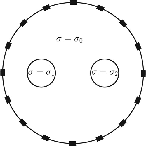In addition, we assume that only skip patterns for current injection are considered such as the current is injected through the jth and $(j+N_e)$th electrodes with $N_e-1$ the number of skipped electrodes. Here, all numerical cases consider only piecewise-constant conductivity fields. Moreover, only circular anomalies are used in the numerical simulations and the conductivities for the anomalies are much higher than those of the background. We utilize a simple EIT solver based on a regularized least-square method for all numerical simulations, although various sophisticated and advanced EIT reconstruction algorithms [2–4] are available, which produce successfully reconstructed conductivity distributions. As an illustration, the schematic of an EIT measurement configuration is shown in Figure 1. The 16 electrodes are attached around the exterior of a chosen imaging object, denoted by Ω, and the electrodes are equidistantly distributed on the object boundary $\mathrm{\partial }\mathrm{\Omega }$; two symmetric anomalies are included in the domain. The values of the conductivity field (σ) for the background, left anomaly and right anomaly are represented by ${\sigma }_m$ (m = 0, 1, 2), respectively. The device injects current through an adjacent pair of electrodes $({\epsilon }_j,{\epsilon }_{j+1}),(j=1,\dots ,N)$ (skip-0 pattern) and simultaneously measures the induced voltages between all neighbouring pairs of electrodes $({\epsilon }_i,{\epsilon }_{i+1})$ for $i=1,\dots ,N$. Note that the convention ${\epsilon }_{N+1}={\epsilon }_1$ is used. Let σ be the electrical conductivity field of $\mathrm{\Omega }\subset {\mathbb{R}}^2$. The electrical potential distribution $u_j$ corresponding to the jth injection current is governed by the following CEM equations [8,33]: (1) $\begin{array}{rl}& \mathrm{\nabla }\cdot \left(\sigma \mathrm{\nabla }{u}_j\right)=0\mathrm{i}\mathrm{n}\mathrm{\Omega },\end{array}$(1) (2) $\begin{array}{rl}& \left(\sigma \mathrm{\nabla }{u}_j\right)\cdot \mathit{n}=0\mathrm{o}\mathrm{n}\mathrm{\partial }\mathrm{\Omega }\setminus \bigcup _{i=1}^N{\epsilon }_i,\end{array}$(2) (3) $\begin{array}{rl}& {\int }_{{\epsilon }_i}\left(\sigma \mathrm{\nabla }{u}_j\right)\cdot \mathit{n}=0\mathrm{f}\mathrm{o}\mathrm{r}\mathit{i}\in \{\mathit{1}\mathit{,}\mathit{2}\mathit{,}\dots \mathit{,}\mathit{N}\}\setminus \{\mathit{j}\mathit{,}\mathit{j}\mathit{+}\mathit{1}\}\mathit{,}\end{array}$(3) (4) $\begin{array}{rl}& u_j+z_i\left(\sigma \mathrm{\nabla }{u}_j\cdot \mathit{n}\right)=U_i^j\mathrm{o}\mathrm{n}{\epsilon }_i\mathrm{f}\mathrm{o}\mathrm{r}i=1,2,\dots ,N,\end{array}$(4) (5) $\begin{array}{rl}& {\int }_{{\epsilon }_j}\left(\sigma \mathrm{\nabla }{u}_j\right)\cdot \mathit{n}\mathrm{d}s=I=-{\int }_{{\epsilon }_{j+1}}\left(\sigma \mathrm{\nabla }{u}_j\right)\cdot \mathit{n}\mathrm{d}s,\end{array}$(5) where $\mathit{n}$ is the outward unit normal vector on $\mathrm{\partial }\mathrm{\Omega }$, $U_i^j$ is the voltage on ${\epsilon }_i$ subject to the jth injection current, $z_i$ is the contact impedance of the ith electrode ${\epsilon }_i$, and I is the amplitude of the injection current between ${\epsilon }_j$ and ${\epsilon }_{j+1}$. Note that this model has been proven to have a unique solution [34]. Assuming that the boundary voltages between all adjacent pairs of electrodes are measured, the measured voltage between the electrode pair $({\epsilon }_i,{\epsilon }_{i+1})$ subject to the jth injection current can be written as (6) $V^{j,i}=U_i^j-U_{i+1}^j,i,j=1,2,\dots ,N,$(6) where $U_{N+1}^j=U_1^j$. The magnitude of the current driven through the jth and the $(j+1)$th electrode is assumed to be normalized to I = 1. Because no current is injected for N−3 voltage data ($V^{j,i},|j-i|>1$, where $V^{1,1-1}=V^{1,N}$) among the N voltage data measured between electrode pairs for each injection current, that is, the normal components of the current density are zeros, it is reasonable to assume $z_i(\sigma \mathrm{\nabla }{u}_j\cdot \mathit{n})\approx 0$ in Equation (4(4) $\begin{array}{rl}& u_j+z_i\left(\sigma \mathrm{\nabla }{u}_j\cdot \mathit{n}\right)=U_i^j\mathrm{o}\mathrm{n}{\epsilon }_i\mathrm{f}\mathrm{o}\mathrm{r}i=1,2,\dots ,N,\end{array}$(4) ). Therefore, we have $u_j{|}_{{\epsilon }_i}=U_i^j$. According to [4], the relationship between σ and $V^{j,i}$ ($|j-i|>1$) can be approximately defined as (7) $V^{j,i}=V^{i,j}={\int }_{\mathrm{\Omega }}\sigma \left(\mathit{r}\right)\mathrm{\nabla }{u}_i\left(\mathit{r}\right)\cdot \mathrm{\nabla }{u}_j\left(\mathit{r}\right)\mathrm{d}\mathit{r},$(7) where $\mathit{r}$ is a position in Ω and $\mathrm{d}\mathit{r}$ is the area element. The voltage data $V^{j,i}$ ($|j-i|\le 1$) are severely affected by the unknown and varying contact impedances. Therefore, Equation (7(7) $V^{j,i}=V^{i,j}={\int }_{\mathrm{\Omega }}\sigma \left(\mathit{r}\right)\mathrm{\nabla }{u}_i\left(\mathit{r}\right)\cdot \mathrm{\nabla }{u}_j\left(\mathit{r}\right)\mathrm{d}\mathit{r},$(7) ) is invalid for $|j-i|\le 1$. For simplicity, we ignore the contact impedances underneath the electrodes in this paper. Then, Equation (7(7) $V^{j,i}=V^{i,j}={\int }_{\mathrm{\Omega }}\sigma \left(\mathit{r}\right)\mathrm{\nabla }{u}_i\left(\mathit{r}\right)\cdot \mathrm{\nabla }{u}_j\left(\mathit{r}\right)\mathrm{d}\mathit{r},$(7) ) holds for $|j-i|\le 1$ as well [4].

Figure 1. Schematic of EIT measurement configuration: a circular domain with two symmetric circular anomalies. Here σ denotes the conductivity field and ${\sigma }_i$ ($i=0,1,2$) represents different values of the conductivity field.

For image reconstruction, the domain Ω is discretized into a computational mesh with elements $p_m$ for $m=1,\dots ,M$. The value of σ for each element is assumed to be the constant ${\sigma }_m$. Hence, Equation (7(7) $V^{j,i}=V^{i,j}={\int }_{\mathrm{\Omega }}\sigma \left(\mathit{r}\right)\mathrm{\nabla }{u}_i\left(\mathit{r}\right)\cdot \mathrm{\nabla }{u}_j\left(\mathit{r}\right)\mathrm{d}\mathit{r},$(7) ) can be re-written as (8) $V^{j,i}=V^{i,j}=\sum _{m=1}^M{\sigma }_m{\int }_{p_m}\mathrm{\nabla }{u}_i\left(\mathit{r}\right)\cdot \mathrm{\nabla }{u}_j\left(\mathit{r}\right)\mathrm{d}\mathit{r}.$(8) The inverse problem of static EIT [35] is to find a best fit of the vector $\mathit{\sigma }=({\sigma }_1,\dots ,{\sigma }_M{)}^T$ such that (9) $\mathit{V}=\mathbb{S}\mathit{\sigma },$(9) with $\mathit{V}=[V^{1,1},\dots ,V^{1,N},V^{2,1},V^{2,2},\dots ,V^{2,N},\dots ,V^{N,1},\dots ,V^{N,N}]$. Here, $\mathbb{S}$ is the sensitivity matrix given by (10) $\mathbb{S}={\left[{\int }_{p_m}\mathrm{\nabla }{u}_i\left(\mathit{r}\right)\cdot \mathrm{\nabla }{u}_j\left(\mathit{r}\right)\mathrm{d}\mathit{r}\right]}_{L\times M},$(10) where $L=N\times N$ and M is selected based on accuracy requirements. Further, $\mathbb{S}$ is pre-computed under the assumption of a homogeneous conductivity distribution (e.g. $\sigma =1$) for the forward model in Equations (1(1) $\begin{array}{rl}& \mathrm{\nabla }\cdot \left(\sigma \mathrm{\nabla }{u}_j\right)=0\mathrm{i}\mathrm{n}\mathrm{\Omega },\end{array}$(1) )–(5(5) $\begin{array}{rl}& {\int }_{{\epsilon }_j}\left(\sigma \mathrm{\nabla }{u}_j\right)\cdot \mathit{n}\mathrm{d}s=I=-{\int }_{{\epsilon }_{j+1}}\left(\sigma \mathrm{\nabla }{u}_j\right)\cdot \mathit{n}\mathrm{d}s,\end{array}$(5) ). The forward problem of reconstructing the conductivity distribution in EIT is to find the voltage V on the surface of the image body by solving Equations (1(1) $\begin{array}{rl}& \mathrm{\nabla }\cdot \left(\sigma \mathrm{\nabla }{u}_j\right)=0\mathrm{i}\mathrm{n}\mathrm{\Omega },\end{array}$(1) )–(5(5) $\begin{array}{rl}& {\int }_{{\epsilon }_j}\left(\sigma \mathrm{\nabla }{u}_j\right)\cdot \mathit{n}\mathrm{d}s=I=-{\int }_{{\epsilon }_{j+1}}\left(\sigma \mathrm{\nabla }{u}_j\right)\cdot \mathit{n}\mathrm{d}s,\end{array}$(5) ) for given σ and I; thus, (11) $\mathit{V}=\mathit{V}(\mathit{r};\sigma ,I).$(11) Note that σ has different values in the anomaly and background as shown in Figure 1. The inverse problem is to find $\tilde{\mathit{\sigma }}$ from the information obtained from Equation (9(9) $\mathit{V}=\mathbb{S}\mathit{\sigma },$(9) ), and can be expressed as (12) $\tilde{\mathit{\sigma }}=\tilde{\mathit{\sigma }}(\mathit{r};\mathbb{S},\mathit{V}).$(12) where $\tilde{\mathit{\sigma }}=({\tilde{\sigma }}_1,\dots ,{\tilde{\sigma }}_M{)}^T$.

2.2. Measurement error

In the present study, we consider the measurement errors caused by the input uncertainties. Generally, there are several kinds of input uncertainties in EIT problems, such as the uncertainty of the electrode contact resistance, body shape and current drive random noise. These uncertainties are then propagated to the measurement data during the experiment or simulation. Thus, various measurement errors are introduced by these input uncertainties. To focus more on the proposed framework, we explore only two kinds of errors in the measurement data; the position error due to the error induced by electrode position perturbation (the difference between the true position of the electrode and the position assumed in the mathematical model); the device error which is treated as an aleatory uncertainty caused by the device itself. Considering the two kinds of measurement errors, we split the measured data into two parts: (13) $\begin{array}{rl}& {\tilde{U}}_i^j=(1+{ϵ}_i^d){\hat{U}}_i^j,\end{array}$(13) (14) $\begin{array}{rl}& {\hat{U}}_i^j=u_j\left({\tilde{\mathit{r}}}_{{\epsilon }_i}\right),{\tilde{\mathit{r}}}_{{\epsilon }_i}={\mathit{r}}_{{\epsilon }_i}+{ϵ}_i^p\mathrm{\Delta }{\mathit{r}}_{{\epsilon }_i},\end{array}$(14) where ${\tilde{U}}_i^j$ is the measured uncertain potential on ${\epsilon }_i$ subject to the jth injection current, ${\hat{U}}_i^j$ is the uncertain potential corresponding to the position perturbation, ${ϵ}_i^d$ is the device error at the ith electrode, $u_j\left({\tilde{\mathit{r}}}_{{\epsilon }_i}\right)$ is the potential obtained at the perturbed position ${\tilde{\mathit{r}}}_{{\epsilon }_i}$ on the boundary, ${\mathit{r}}_{{\epsilon }_i}$ is the true position of electrode ${\epsilon }_i$, ${\mathit{ϵ}}^p=({ϵ}_1^p,\dots ,{ϵ}_N^p)$ is the position error, and $\mathrm{\Delta }{\mathit{r}}_{{\epsilon }_i}$ is the distance along the boundary surface between two electrodes. Then, the trial voltage $V_T^{j,i}$ in the inverse problem can be computed as (15) $V_T^{j,i}={\tilde{U}}_i^j-{\tilde{U}}_{i+1}^j,i,j=1,2,\dots ,N.$(15) Throughout this paper, we denote the random vector $\mathit{ϵ}=({ϵ}_1,\dots ,{ϵ}_{2N})=({ϵ}_1^p,\dots ,$ ${ϵ}_N^p,{ϵ}_1^d,\dots ,{ϵ}_N^d)$ as the measurement error, where the first N elements are the position errors corresponding to perturbation of the electrodes ${\epsilon }_1$ to ${\epsilon }_N$, and the remaining elements are device errors. In addition, ${ϵ}_i^d$ and ${ϵ}_i^p$ are considered as ‘uncertain variables’ in this study. They are bounded in nature. However, the precise intervals for these errors are usually unknown. Therefore we specify a slightly larger interval for each error according to basic information and our experience. The value of the error belongs to the specified distribution (e.g. normal distribution specified for the test cases in Section 4), which causes the measurement data to be uncertain in the following regularization method and further affects the final results.

3. Proposed framework

3.1. Regularized least-squares method

Image reconstruction in EIT is a nonlinear and ill-posed problem. Various regularization methods have been proposed [3,4] in order to resolve the solution instability. As the objective of the present study is not related to the inverse solver, a common Tikhonov regularization approach [36] is adopted for simplicity. The general form of a Tikhonov regularization approach to the EIT inverse solution can be written as [5,36] (16) $\tilde{\mathit{\sigma }}=\mathrm{a}\mathrm{r}\mathrm{g}\mathrm{m}\mathrm{i}\mathrm{n}\parallel \mathbb{S}\mathit{\sigma }-\mathit{V}{\parallel }^2+\alpha \parallel \mathit{L}\mathit{\sigma }{\parallel }^2,$(16) where α is the regularization parameter and $\mathit{L}$ is an appropriate regularization matrix used to penalize a measure of the roughness of $\mathit{\sigma }$. The most frequently used regularization matrices in EIT are the identity matrix and those corresponding to the first and second difference operators [37–39]. (For more information, refer to [3,4,6] and the references therein.) Specifically, the EIT solver used in this paper is a modified version of the ones used in [40,41].

3.2. Shape detection indices

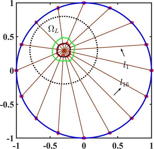
As discussed in Section 2.2, the sizes of the errors corresponding to various measurements are unknown in a practical situation. A wide range of added error values are usually specified, which might inevitably yield some visually poor reconstructions in the experiments. We consider poor reconstructions as failures, and others are treated as successful reconstructions. The structural similarity index (SSIM) [42] may be a good choice for classifying each reconstruction as a success or a failure. The SSIM assesses the visual impact of the three characteristics of an image–luminance, contrast and structure–which can effectively evaluate the degree of the structural deviation between two images. However, as the exact position and geometry of the anomaly are assumed in the present study, we wish to develop more locally defined indices to further study the influence of the measurement errors on the image reconstruction. More precisely, two detection indices are introduced in this study–the contrast index ci and the similarity index si. The index ci is used to measure the contrast between the anomaly and the background area as well as to determine whether a given reconstruction is successful or not. si is used to measure the similarity between the detected shape and the exact shape of the anomaly; hence, the reconstruction performance can be determined.

To define the two indices, we first construct lines $l_i$ between the electrodes and the centre of the anomaly, as shown in Figure 2. Here, (17) $l_i:y-y_0=k_i(x-x_0),k_i=\frac{y_i-y_0}{x_i-x_0},i=1,2,\dots ,N,$(17) where N is the number of electrodes, $(x_0,y_0)$ are the coordinates of the centre of the anomaly, and $(x_i,y_i)$ are electrode coordinates. The local minimum values of the conductivity are then calculated along the lines $l_i$ within the following domain: (18) ${\mathrm{\Omega }}_L=\left\{\right(x,y)|\sqrt{(x-x_0{)}^2+(y-y_0{)}^2}\le r_L\},$(18) where $r_L$ is the radius properly selected based on the size of the background area. Considering the shape constructed by the local minimum values as an approximation of the shape of the anomaly, the maximum values of the derivative of conductivity in the direction of $l_i$ are computed within ${\mathrm{\Omega }}_L$. Because the derivative of the conductivity reflects the contrast between the background of the domain and the anomaly, and the similarity between the reconstructed image and the original anomaly is reflected by the difference in their geometries, ci and si can be defined using the maximum values and their positions, as follows. (19) $\begin{array}{rl}& \mathrm{c}\mathrm{i}=\frac{\frac{1}{N}\sum _{i=1}^{N}D{\sigma }_i}{\mathrm{c}\mathrm{l}},\end{array}$(19) (20) $\begin{array}{rl}& \mathrm{s}\mathrm{i}=\frac{1}{N}\sum _{i=1}^N\frac{{\mathrm{d}\mathrm{i}\mathrm{s}}_i}{r_a}.\end{array}$(20) Note that $\mathrm{c}\mathrm{l}$ in Equation (19(19) $\begin{array}{rl}& \mathrm{c}\mathrm{i}=\frac{\frac{1}{N}\sum _{i=1}^{N}D{\sigma }_i}{\mathrm{c}\mathrm{l}},\end{array}$(19) ) is a normalization constant determined by the conductivity field (e.g.$\mathrm{c}\mathrm{l}=|{\tilde{\sigma }}_{max}-{\tilde{\sigma }}_{min}|$), and $D{\sigma }_i=max\left\{\frac{\mathrm{d}\sigma }{\mathrm{d}{l}_i}\right\}$ is the maximum derivative of the conductivity in the direction of $l_i$ in the region constructed by the local minimum points of the conductivity. In addition, in the definition of si, $r_a$ is the anomaly radius and ${\mathrm{d}\mathrm{i}\mathrm{s}}_i=\sqrt{(x{d}_i-x_0{)}^2+(y{d}_i-y_0{)}^2}$ is the distance between the reconstructed shape and the anomaly surface, where $(x{d}_i,y{d}_i)$ are the coordinates of the maximum derivative of conductivity in the direction of line $l_i$.

Figure 2. Illustration of shape detection indices. Red circles: electrodes; brown lines: 16 lines $l_i$ from centre of the anomaly to the electrodes; green and red outlines: shapes constructed by local minimum conductivities and maximum derivatives of conductivity in the direction of line $l_i$, respectively; black line: anomaly boundary. Note that the figure is based on the reconstructed image for a single anomaly in a circular domain without measurement errors.

Note that the optimum values of these two indices cannot be defined. However, there should be some limits on the values of these indices. If the two images being compared are identical, ci and si should be same for both reconstructed images. For example, considering the image reconstructed using the measurement data without errors as the reference image, any other reconstructed image that is identical to the reference image has same ci and si indices. We defined these two indices to measure the reconstruction quality of the EIT solver used in this study. If these two indices satisfy some conditions, we can consider the reconstruction to be successful. This means that the reconstructed image can show a contrast between an anomaly and the background such that one can identify an anomaly in the reconstructed image. Then, we can quantify the influence of the measurement errors on the image reconstruction by the global sensitivity analysis of these two indices with regard to the measurement errors. A more precise use of ci and si is discussed in Section 4.1.

3.3. Polynomial chaos expansion (PCE)

To reduce the complexity of the computation and statistical analysis, we construct a surrogate model for the reconstructed conductivity field $\tilde{\sigma }$ by means of PCE [29,30]. The basic purpose of the PCE is to use orthogonal polynomials in terms of random variables to approximate the functions of those random variables. A continuous surrogate model (response surface) is recovered to a finite order of the spectral decomposition. For the element $p_m$ in the domain Ω, the reconstructed conductivity ${\tilde{\sigma }}_m$ can be written as (21) $\begin{array}{rl}& {\tilde{\sigma }}_m\left(\mathit{ϵ}\right)=\sum _{k=0}^{K_m^{\sigma }-1}{c}_k^m{\mathrm{\Psi }}_k\left(\mathit{\xi }\right)+{\epsilon }_{K_m^{\sigma }},\mathrm{f}\mathrm{o}\mathrm{r}m=1,\dots ,M,\\ & {ϵ}_i=\sum _{l=0}^{K_i^{ϵ}-1}{\alpha }_l^m{\mathrm{\Psi }}_l\left(\mathit{\xi }\right)+{\epsilon }_{K_i^{ϵ}},\mathrm{f}\mathrm{o}\mathrm{r}i=1,\dots ,2N\end{array}$(21) with respect to the canonical orthogonal polynomials ${\mathrm{\Psi }}_k\left(\mathit{\xi }\right)$ of an independent-component random vector $\mathit{\xi }$, where ${\epsilon }_{K_m^{\sigma }}$ and ${\epsilon }_{K_i^{ϵ}}$ are truncation errors. In the present study, the distribution of the random vector $\mathit{ϵ}$ is assumed to normal, i.e. a vector of independent and identically distributed (i.i.d.) Gaussian random variables with mean ${\mu }_{ϵ}$ and standard deviation $a_{ϵ}$. Thus ${\mathrm{\Psi }}_k\left(\mathit{\xi }\right)$ are chosen to be Hermite polynomials that are orthogonal with respect to the probability density function (PDF) of $\mathit{\xi }$, ${\pi }_{\mathit{\xi }}\left(\mathit{\xi }\right)$. The components of $\mathit{\xi }$ are i.i.d. standard normal variables with zero mean and unity standard deviation, yielding a value of $K_i^{ϵ}$ equal to 1 and ${\epsilon }_{K_i^{ϵ}}=0$. Thus, we have ${ϵ}_i=a_{ϵ}{\xi }_i+{\mu }_{ϵ}$. Further, $K_m^{\sigma }$ is defined as $K_m^{\sigma }=(q+d)!/q!d!$, where d is the dimension of the random space and q is the maximum polynomial order of the expansion selected according to the accuracy requirements. The orthogonality of the polynomial bases is written as (22) $\mathbb{E}\left[{\mathrm{\Psi }}_k\left(\mathit{\xi }\right){\mathrm{\Psi }}_l\left(\mathit{\xi }\right)\right]=⟨{\mathrm{\Psi }}_k\left(\mathit{\xi }\right),{\mathrm{\Psi }}_l\left(\mathit{\xi }\right)⟩={\int }_{\mathit{\xi }}{\mathrm{\Psi }}_k\left(\mathit{\xi }\right){\mathrm{\Psi }}_l\left(\mathit{\xi }\right){\pi }_{\mathit{\xi }}\left(\mathit{\xi }\right)\mathrm{d}\mathit{\xi }=⟨{\mathrm{\Psi }}_k^2⟩{\delta }_{kl},$(22) where ${\delta }_{kl}$ is the Kronecker delta; ${\mathrm{\Psi }}_k\left(\mathit{\xi }\right)={\psi }_{k_1}\left({\xi }_1\right)\cdots {\psi }_{k_d}\left({\xi }_d\right),k=k_1+\cdots +k_d,0\le k\le p$, ψ are the univariate polynomials; ${\pi }_{\mathit{\xi }}\left(\mathit{\xi }\right)=\prod _{k=0}^d{\pi }_k\left({\xi }_k\right)$; ${\pi }_k\left({\xi }_k\right)$ is the weight function corresponding to ${\xi }_k$ distribution.

In the framework proposed in the present study, a regression-based non-intrusive method is used to obtain the PCE in Equation (21(21) $\begin{array}{rl}& {\tilde{\sigma }}_m\left(\mathit{ϵ}\right)=\sum _{k=0}^{K_m^{\sigma }-1}{c}_k^m{\mathrm{\Psi }}_k\left(\mathit{\xi }\right)+{\epsilon }_{K_m^{\sigma }},\mathrm{f}\mathrm{o}\mathrm{r}m=1,\dots ,M,\\ & {ϵ}_i=\sum _{l=0}^{K_i^{ϵ}-1}{\alpha }_l^m{\mathrm{\Psi }}_l\left(\mathit{\xi }\right)+{\epsilon }_{K_i^{ϵ}},\mathrm{f}\mathrm{o}\mathrm{r}i=1,\dots ,2N\end{array}$(21) ), in which the PCE coefficients are estimated by minimizing the mean squared error of the response approximation. This method has been widely accepted and studied in recent years owing to its satisfactory performance (see [43–45]). We also apply a sparse PCE model to mitigate the extremely large computation cost due to the high dimensionality of the random space. Recently, Blatman and Sudret [45] successfully applied the least angle regression (LAR) algorithm [46] to obtain sparse PCE models that are accurate even with very small experimental designs. Hence, the $l_1$ regularized least-square minimization problem is solved as follows: (23) ${\mathit{c}}^m=\mathrm{a}\mathrm{r}\mathrm{g}\underset{{\hat{\mathit{c}}}^m}{min}\mathbb{E}\left[{\left(\mathbf{\Psi }\left(\mathit{\xi }\right){\hat{\mathit{c}}}^m-{\tilde{\sigma }}_m\left(\mathit{\xi }\right)\right)}^2\right]+\lambda \parallel {\hat{\mathit{c}}}^m{\parallel }_1,m=1,2,\dots ,M,$(23) where ${\mathit{c}}^m=(c_0^m,\dots ,c_{K_m^{\sigma }-1}^m)$, λ is a regularization parameter, and $\parallel \cdot {\parallel }_1$ is the $l_1$ norm that sums the absolute element of a vector. In this study, the LAR algorithm is adopted to solve Equation (23(23) ${\mathit{c}}^m=\mathrm{a}\mathrm{r}\mathrm{g}\underset{{\hat{\mathit{c}}}^m}{min}\mathbb{E}\left[{\left(\mathbf{\Psi }\left(\mathit{\xi }\right){\hat{\mathit{c}}}^m-{\tilde{\sigma }}_m\left(\mathit{\xi }\right)\right)}^2\right]+\lambda \parallel {\hat{\mathit{c}}}^m{\parallel }_1,m=1,2,\dots ,M,$(23) ).

Furthermore, the leave-one-out cross validation error (${\epsilon }_{LOO}$) is considered in order to evaluate the predictive ability of a given PCE metamodel; ${\epsilon }_{LOO}$ has been proven to perform well for PCE accuracy estimation in [45] and can be defined as (24) ${\epsilon }_{LOO}=\frac{\sum _{i=1}^{N_s}{\left({\tilde{\sigma }}_m\left({\mathit{\xi }}_i\right)-{\sigma }_m^{PCE\setminus i}\left({\mathit{\xi }}_i\right)\right)}^2}{\sum _{i=1}^{N_s}{\left({\tilde{\sigma }}_m\left({\mathit{\xi }}_i\right)-{\mu }_{\sigma }\right)}^2},{\mu }_{\sigma }=\frac{1}{N_s}\sum _{i=1}^{N_s}{\tilde{\sigma }}_m\left({\mathit{\xi }}_i\right),$(24) where ${\tilde{\sigma }}_m$ is the reconstructed conductivity for element $p_m$ and ${\sigma }_m^{PCE\setminus i}$ is the corresponding PCE metamodel constructed based on $N_s$ samples of uncertain input variables, excluding the ith sample ${\mathit{\xi }}_i$; the samples are generated using the Latin hypercube sampling (LHS) method [47].

3.4. Global sensitivity analysis based on Sobol' indices

Variance-based sensitivity analysis is a form of global sensitivity analysis (GSA) that depends on decomposition of the output variance into the contributions of different components; i.e. marginal effects and input factor interactions. Variance decomposition methods that yield the well-known Sobol' indices [48] are recognized as accurate techniques for global sensitivity analysis. In the framework proposed in the present study, Sobol' indices are used to rank the relative contributions of each input uncertain parameter to the total uncertainty in the output quantities of interest. These indices can be derived via the Sobol' decomposition with the PCE coefficients calculated using Equation (23(23) ${\mathit{c}}^m=\mathrm{a}\mathrm{r}\mathrm{g}\underset{{\hat{\mathit{c}}}^m}{min}\mathbb{E}\left[{\left(\mathbf{\Psi }\left(\mathit{\xi }\right){\hat{\mathit{c}}}^m-{\tilde{\sigma }}_m\left(\mathit{\xi }\right)\right)}^2\right]+\lambda \parallel {\hat{\mathit{c}}}^m{\parallel }_1,m=1,2,\dots ,M,$(23) ). Based on the orthogonality property of the polynomial basis, the total variance can be expressed as (25) $D_m=\sum _{k=1}^{K_m^{\sigma }-1}(c_k^m{)}^2<{\mathrm{\Psi }}_k^2(\mathit{\xi })>.$(25) Then, the total variance can be decomposed as [49,50] (26) $D_m=\sum _{k_1=1}^{k_1=d}{D}_m^{k_1}+\sum _{1\le k_1\le k_2\le d}^{k_1=d-1}{D}_m^{k_1,k_2}+\sum _{1\le k_1\le k_2\le k_3\le d}^{k_1=d-2}{D}_m^{k_1,k_2,k_3}+\cdots +D_m^{1,2,\dots ,d},$(26) where the partial variance ($D_m^{k_1,\dots ,k_s}$) is given by (27) $D_m^{k_1,\dots ,k_s}=\sum _{\mathit{\tau }\in \{k_1,\dots ,k_s\}}(c_{\mathit{\tau }}^m{)}^2<{\mathrm{\Psi }}_{\mathit{\tau }}^2(\mathit{\xi })>,1\le k_1<\dots <k_s\le d.$(27) The Sobol' indices can be represented by the relations (28) $S_m^{k_1,\dots ,k_s}=\frac{D_m^{k_1,\dots ,k_s}}{D_m}\mathrm{a}\mathrm{n}\mathrm{d}\sum _{k_1=1}^{k_1=d}{S}_m^{k_1}+\sum _{1\le k_1\le k_2\le d}^{k_1=d-1}{S}_m^{k_1,k_2}+\cdots +S_m^{1,2,\dots ,d}=1.$(28) Further, the total Sobol' indices $S_{T_i}$ of an input parameter k can be defined as [49,51] (29) $S_m^{T_k}=\sum _{{\mathcal{A}}_k}\frac{D_m^{k_1,\dots ,k_s}}{D_m},{\mathcal{A}}_k=\left\{\right(k_1,\dots ,k_s):\mathrm{\exists }l,1\le l\le s,k_l=k\}.$(29) Note that the Sobol' indices measure the sensitivity to the individual contribution of each input uncertain variable ($S_m^{k_1}$) as well as the interaction contributions ($S_m^{k_1,k_2},S_m^{k_1,k_2,k_3},\dots$). Similar to the Sobol' indices, the total Sobol' indices measure the sensitivity to the total contribution of each input uncertain variable ($S_m^{T_k}$).

The two detection indices in Equations (19(19) $\begin{array}{rl}& \mathrm{c}\mathrm{i}=\frac{\frac{1}{N}\sum _{i=1}^{N}D{\sigma }_i}{\mathrm{c}\mathrm{l}},\end{array}$(19) ) and (20(20) $\begin{array}{rl}& \mathrm{s}\mathrm{i}=\frac{1}{N}\sum _{i=1}^N\frac{{\mathrm{d}\mathrm{i}\mathrm{s}}_i}{r_a}.\end{array}$(20) ) (ci and si) are utilized to identify a successful detection, and to reduce the epistemic uncertainty in the specified measurement error distributions. When GSA is conducted for the conductivity reconstruction with the constraint of successful detection, the parameter space cannot be considered as a d-dimensional hypercube. The space can be formed in any shape (including disconnected domains) depending on the constraints that impose structural dependencies between the input uncertain variables; this implies that the above PCE-based GSA may be inappropriate for such a case. Thus, we adopt a constrained GSA (cGSA) approach [32] with Monte Carlo (MC) or quasi-MC estimators based on acceptance-rejection sampling for the Sobol' sensitivity indices.

Let $f\left(\mathit{\xi }\right)$ be a model function (e.g. $f={\tilde{\sigma }}_m$) depending on the input vector $\mathit{\xi }=({\xi }_1,\dots ,{\xi }_d)\in H^d$ (hypercube space). By referring to [32], the Sobol' indices (28(28) $S_m^{k_1,\dots ,k_s}=\frac{D_m^{k_1,\dots ,k_s}}{D_m}\mathrm{a}\mathrm{n}\mathrm{d}\sum _{k_1=1}^{k_1=d}{S}_m^{k_1}+\sum _{1\le k_1\le k_2\le d}^{k_1=d-1}{S}_m^{k_1,k_2}+\cdots +S_m^{1,2,\dots ,d}=1.$(28) ) and the total Sobol' indices (29(29) $S_m^{T_k}=\sum _{{\mathcal{A}}_k}\frac{D_m^{k_1,\dots ,k_s}}{D_m},{\mathcal{A}}_k=\left\{\right(k_1,\dots ,k_s):\mathrm{\exists }l,1\le l\le s,k_l=k\}.$(29) ) in the constraint domain $Q^d\subset H^d$ can be re-defined as follows: (30) $\begin{array}{rl}& S_m^y=\frac{1}{D_m}\left[{\int }_{H^s}\frac{\left[{\int }_{H^{d-s}}f\right(\mathit{y},\mathit{z}\left)p^Q\right(\mathit{y},\mathit{z})\mathrm{d}\mathit{z}{]}^2}{p^Q\left(\mathit{y}\right)}\mathrm{d}\mathit{y}-f_0^2\right],\end{array}$(30) (31) $\begin{array}{rl}& S_m^{T_y}=\frac{1}{2D_m}{\int }_{Q^d}{\int }_{Q^s}\left[f\right(\mathit{y},\mathit{z})-f({\mathit{y}}^{\mathbf{\prime }},\mathit{z}\left){]}^2{p}^Q\right(\mathit{y},\mathit{z})\frac{p^Q({\mathit{y}}^{\mathbf{\prime }},\mathit{z})}{p^Q\left(\mathit{y}\right)}\mathrm{d}\mathit{y}\mathrm{d}{\mathit{y}}^{\mathbf{\prime }}\mathrm{d}\mathit{z},\end{array}$(31) where $\mathit{y}=({\xi }_1,\dots ,{\xi }_s)$, $\mathit{z}=({\xi }_{s+1},\dots ,{\xi }_d)$, $\mathit{\xi }=(\mathit{y},\mathit{z})$, and $\frac{p^Q(\mathit{y},\mathit{z})}{p^Q\left(\mathit{y}\right)}=p^Q(\mathit{y},\overline{\mathit{z}}|\mathit{y})$ is the conditional PDF. Note that, for simplicity, $Q^d$ is represented by Q when appearing as a superscript. Furthermore, $p^Q$ is the marginal PDF of the subset of inputs y, and $p^Q(\mathit{y},\mathit{z})$ is the joint PDF defined as (32) $p^Q(\mathit{y},\mathit{z})=\frac{p(\mathit{y},\mathit{z})I^Q(\mathit{y},\mathit{z})}{\overline{I}}.$(32) Here, $p(\mathit{y},\mathit{z})$ is the joint PDF in $H^d$ and (33) $\overline{I}={\int }_{Q^d}p(\mathit{y},\mathit{z})\mathrm{d}\mathit{y}\mathrm{d}\mathit{z}={\int }_{H^d}p(\mathit{y},\mathit{z})I^Q(\mathit{y},\mathit{z})\mathrm{d}\mathit{y}\mathrm{d}\mathit{z}.$(33) The indicator function $I^Q(\mathit{y},\mathit{z})$ of the subset $Q^d$ is defined as (34) $I^Q(\mathit{y},\mathit{z})=\left\{\begin{array}{ll}1& (\mathit{y},\mathit{z})\in Q^d,\\ 0& (\mathit{y},\mathit{z})\notin Q^d.\end{array}\right.$(34) Combining the above UQ methods and EIT reconstruction techniques, we propose a framework to quantify the effect of the measurement errors on the EIT reconstruction problems. The overall algorithm of the proposed framework is presented in Algorithm 1.

4. Results and discussion

This section describes the investigations of the performance of the proposed framework for three EIT reconstruction problems: a single anomaly in a circular domain, two anomalies in a circular domain, and two anomalies in a body-like domain. Throughout this section, the normalization constant $\mathrm{c}\mathrm{l}$ for ci in Equation (19(19) $\begin{array}{rl}& \mathrm{c}\mathrm{i}=\frac{\frac{1}{N}\sum _{i=1}^{N}D{\sigma }_i}{\mathrm{c}\mathrm{l}},\end{array}$(19) ) is defined as $\mathrm{c}\mathrm{l}=\sum _{i=1}^{N_t}|{\sigma }_{max}^i-{\sigma }_{min}^i|$, where $N_t$ is the number of samples in the cGSA.

4.1. Quantifying effects of device errors on EIT reconstruction

We considered a case in which the measurement errors consisted of device errors only. Thus, the relationship between the measured uncertain potential and input measurement error can be simplified as (35) ${\tilde{U}}_i^j=(1+{ϵ}_i)U_i^j,$(35) where ${ϵ}_i$ is the device error corresponding to the electrode ${\epsilon }_i$ and the random vector is denoted as $\mathit{ϵ}=({ϵ}_1,\dots ,{ϵ}_N)$.

4.1.1. Single anomaly in circular domain

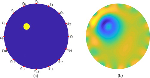
First, we considered a case involving a single circular anomaly in a circular domain with device errors, as illustrated in Figure 3(a). The numerically simulated domain was a circle with radius of 1 cm and the radius of the circular inclusion was 0.1 cm. The electrodes used in this case were assumed to be points along the computational domain boundary. The value of the conductivity field used for the background was 1 S/m, and that of the anomaly was set to 10 S/m. Before proceeding, we reconstructed the conductivity field for the case without measurement errors using the inverse solver, which provided a reasonable reconstructed image as shown in Figure 3(b). As the measurement error distributions were mostly unknown owing to lack of information, it was necessary to specify a prior distribution for each error according to the physical facts and EIT expert opinions. The device errors ${ϵ}_i$ corresponding to different electrodes were assumed to be i.i.d. normal distributions with zero mean and standard deviation $s_d^i$. To define an appropriate set of parameters for PCE, a set of device errors $\{{\mathit{ϵ}}^{\left(j\right)}{\}}_{j=1}^{N_s}$ was generated using the LHS method with $s_d^i=a$. 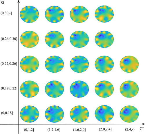The value of a was selected from the interval $[0.015,0.03]$, for simplicity. As the selection of a depends on the EIT reconstruction results, we defined an appropriate detection criterion for successful reconstruction by performing a large number of trials for all test EIT problems. For example, Figure 4 shows several reconstructed images of different detection indices for the case of a single anomaly in a circular domain. The reconstructed images are distributed based on the ci (horizontal direction) and si (vertical direction) values. When the ci of the reconstructed images was less than 1.2, it was difficult to distinguish the anomaly in the conductivity distribution. As ci increased, the difference in the conductivity between the anomaly and background became larger, leading to a clearer contrast. Furthermore, the detected shape attained greater similarity to the original anomaly for a smaller si. Note that the reconstructed images for $\mathrm{c}\mathrm{i}>2.4$ and $\mathrm{s}\mathrm{i}>0.26$ are not shown in Figure 4, because si is generally very small for a large ci. In summary, ci should be larger than 1.2 to obtain a successful reconstruction and the value of si should be kept as small as possible to detect a shape similar to that of the true anomaly. Therefore, in this study, $\mathrm{c}\mathrm{i}>1.2$ was used as the detection criterion for successful reconstructions.

Figure 3. EIT reconstruction for single circular anomaly in circular domain: (a) model configuration and (b) reconstruction without measurement errors.

Based on the conductivity fields obtained from the inverse problem solver, the corresponding PCEs were constructed by solving Equation (23(23) ${\mathit{c}}^m=\mathrm{a}\mathrm{r}\mathrm{g}\underset{{\hat{\mathit{c}}}^m}{min}\mathbb{E}\left[{\left(\mathbf{\Psi }\left(\mathit{\xi }\right){\hat{\mathit{c}}}^m-{\tilde{\sigma }}_m\left(\mathit{\xi }\right)\right)}^2\right]+\lambda \parallel {\hat{\mathit{c}}}^m{\parallel }_1,m=1,2,\dots ,M,$(23) ) via the LAR method. Here, the maximum order of the polynomial basis (q) and the number of samples ($N_s$) were iteratively determined by increasing q or $N_s$, so that the leave-one-out cross validation error satisfied a stopping criterion, i.e. ${\epsilon }_{LOO}<{10}^{-10}$. Hence, it was found that the PCE parameters q = 1 and $N_s=50$ were appropriate to reconstruct the conductivity fields obtained from the inverse solver.

Figure 4. Reconstructed images of different detection indices for the case of a single anomaly in a circular domain.

Referring to Figure 4, some reconstructed images failed to exhibit meaningful detection of the anomaly depending on the measurement errors related to the electrode. For a reliable sensitivity analysis of the measurement errors, we further investigated the effect of the prior distributions of the measurement device errors on the success rates of anomaly detection in the reconstruction. As discussed in Section 3.2, the successful case was determined based on the shape detection criterion ($\mathrm{c}\mathrm{i}>1.2$), and the success rate was defined as the ratio of the number of successful reconstructions to the number of trials ($N_t$). To this end, several PCEs with q = 1 and $N_s=50$ were constructed based on the device errors generated from the i.i.d. normal distributions with $s_d^i=a$, where 13 different values of a were selected from the interval $[0.015,0.03]$. The detection indices were then estimated from the PCEs of the conductivity field. Later, the success rates were calculated based on $N_t={10}^5$ trials involving randomly generated device errors with the LHS method.

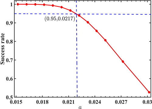
Figure 5 indicates that the reconstruction success rate decreased as a increased. Note that the success rate was found to be 1.0 when a was less than 0.016. This implies that the enclosed anomaly was identified with $100\mathrm{\%}$ probability based on the present detection indices in the reconstructed images for ${10}^5$ trials. In statistics, if the probability of an event is very small or an event is very unlikely to occur in a single experiment, the event can be considered a small-probability event [52]. In general, two widely accepted probability thresholds, 0.01 and 0.05, are used for a small probability event. Here, $5\mathrm{\%}$ failure probability in the reconstruction was taken as the criterion for a small-probability event. As shown in Figure 5, a was required to be less than 0.0217 for a successful reconstruction to be obtained with $95\mathrm{\%}$ probability in the employed EIT model. This means that the percentage of perturbations in the measured data due to the device errors was required to be less than approximately $7\mathrm{\%}$ for successful reconstruction with $95\mathrm{\%}$ probability.

Figure 5. Success rates depending on standard deviation of the device error a. Success rate denotes the rate of successful image reconstruction in ${10}^5$ trials. The blue dotted lines are used to show the position of the case with $95\mathrm{\%}$ success rate, which is denoted by the intersection point between the dotted lines and red solid line.

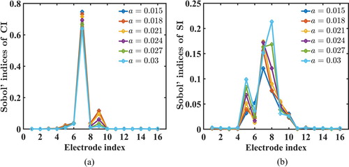
We further performed cGSA of the detection indices based on the Sobol' indices in Equation (30(30) $\begin{array}{rl}& S_m^y=\frac{1}{D_m}\left[{\int }_{H^s}\frac{\left[{\int }_{H^{d-s}}f\right(\mathit{y},\mathit{z}\left)p^Q\right(\mathit{y},\mathit{z})\mathrm{d}\mathit{z}{]}^2}{p^Q\left(\mathit{y}\right)}\mathrm{d}\mathit{y}-f_0^2\right],\end{array}$(30) ) so as to investigate the effect of the measurement errors on the EIT reconstruction. Figure 6(a,b) show the ci and si sensitivities to the device error for different values of a, respectively. With decreasing a, the Sobol' index distribution for ci converged to that of the case for a = 0.015 (i.e. $100\mathrm{\%}$ probability of success). Furthermore, the device error at the 7th electrode, which was closest to the anomaly, was found to be the most influential factor as regards the ci variation. The device errors at the neighbouring electrodes (i.e. electrodes 5−9) of the 7th electrode were slightly influential as regards the ci variation, whereas the indices were almost insensitive to the errors at other electrodes. Figure 6(b) indicates that the Sobol' index distribution for si converged gradually to that of the case for a = 0.015 as the device errors decreased. Similar to ci, it was found that the device error at the 7th electrode had the greatest influence on the si variation. However, the Sobol' indices of si at the electrodes close to the anomaly (i.e. electrodes 4−10) were relatively large and the distribution was wider compared to that of ci. This implies that si is more non-locally sensitive to the device errors at the electrodes close to the anomaly than ci. Thus, based on the cGSA, the quality of an EIT reconstruction mostly depends on the device errors at the electrodes close to the anomaly. Further, the device error corresponding to the electrode closest to the anomaly has the greatest influence on the EIT reconstruction.

Figure 6. Results of cGSA for shape detection indices of the case with single anomaly in circular domain depending on standard deviation of device error a: (a) CI and (b) SI.

4.1.2. Two anomalies in circular domain

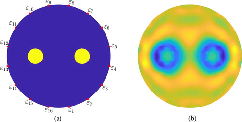
We considered two circular anomalies in a circular domain, as shown in Figure 7 so as to investigate effects of the measurement error on EIT reconstruction involving interference by multiple objects. Figure 7(a) shows that two anomalies were placed symmetrically with respect to the centre of the circular domain, while 16 electrodes were placed equidistantly along the domain boundary. The numerically simulated domain was a circle with radius of 1 cm and the radii of the two circular inclusions were 0.1 cm. The electrodes used in this case were assumed to be points along the computational domain boundary. The conductivity used for the background was 1 S/m, and that for the anomalies was 10 S/m. Using the inverse solver discussed in Section 3.1, a conductivity field was reconstructed without considering the measurement errors. Figure 7(b) indicates that the two anomalies were clearly captured in the reconstructed image using the present inverse solver.

Figure 7. EIT reconstruction of two circular anomalies in circular domain: (a) model configuration and (b) reconstruction without measurement errors.

In a similar approach to that used for the single-anomaly case, we performed a preliminary test to obtain a set of parameters for PCE and to determine the level of device errors for a reliable cGSA. Hence, q = 1 and $N_s=50$ were chosen as the PCE parameters and a = 0.03 was used for the device errors. With these settings, a success rate of more than 0.95 for detection of the two anomalies was achieved for $N_t={10}^5$ trials according to the ci criterion. The cGSA results for the ci and si of the two anomalies are shown in Figure 8. In comparison with Figure 6, the Sobol' indices for ci are much smaller in the case with two anomalies than in the case with one anomaly. This is because the interaction contributions among the measurement errors in the case with two anomalies are larger than those in the case with one anomaly case are. Figures 6 and 8 show the main Sobol' indices. 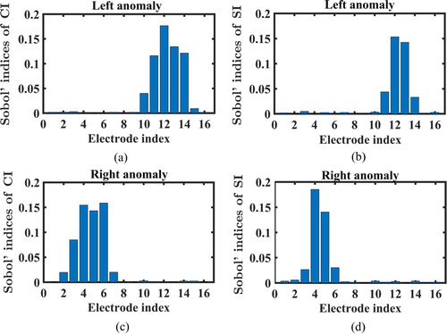As shown in Equation (28(28) $S_m^{k_1,\dots ,k_s}=\frac{D_m^{k_1,\dots ,k_s}}{D_m}\mathrm{a}\mathrm{n}\mathrm{d}\sum _{k_1=1}^{k_1=d}{S}_m^{k_1}+\sum _{1\le k_1\le k_2\le d}^{k_1=d-1}{S}_m^{k_1,k_2}+\cdots +S_m^{1,2,\dots ,d}=1.$(28) ), the summation of all Sobol' indices is 1. Hence, if the interaction contributions among the measurement errors become large, the main contribution of each error becomes smaller. Similar to the single-anomaly case, Figure 8 shows that the Sobol' indices for ci and si were relatively large at the electrodes close to each anomaly (i.e. electrodes 10–14 and 2–6 for the left and right anomalies, respectively), while the distributions of the indices for the two anomalies were roughly symmetric with respect to the vertical centre line in the domain. It was observed that the errors at the electrode closest to each anomaly (i.e. electrodes 12 and 4 for the left and right anomalies, respectively) had the greatest influence on the indices. Further, the sum of all Sobol' indices of si was smaller than that of ci. For the left anomaly, the sums for ci and si were estimated as 0.6126 and 0.3988, respectively. This implies that variations of si were more strongly affected by interactive device errors than those of ci.

Figure 8. Results of cGSA for shape detection indices of the case with two anomalies in circular domain: (a) CI and (b) SI of left anomaly, and (c) CI and (d) SI of right anomaly. The electrode index is described in Figure 7(a).

4.2. Quantifying effects of position and device errors on EIT reconstruction

When both position and device errors are considered, the relationship between the measurement error and conductivity becomes highly nonlinear, and the dimension of the random space increases to 32. All these changes increase the computational cost and complexity. To obtain reasonable results with low computational costs, settings of ${\epsilon }_{LOO}^T=1.0\times {10}^{-2}$, $N_s=5000$, and q = 6 were employed in the following part of the study.

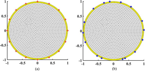
As electrode perturbation yields position errors for each trial, the corresponding finite element method (FEM) mesh should be adapted or newly generated to solve the forward problem in Equation (11(11) $\mathit{V}=\mathit{V}(\mathit{r};\sigma ,I).$(11) ). As an example, the original and adapted FEM meshes are shown in Figure 9(a,b), respectively. Note that the position errors were randomly generated from the normal distribution $N(0,{0.3}^2)$. Figure 9(a) shows the original FEM mesh, where the original electrodes (red plus signs) were equidistantly located at certain nodes on the boundary. Figure 9(b) shows that the perturbed electrodes (blue asterisks) were newly placed depending on the position errors. The nodes were then re-arranged on the boundary (yellow region), while the positions of the other nodes remained unchanged.

Figure 9. Meshes used in forward solver: (a) original and (b) adaptive meshes. Note that the red plus signs and blue asterisks denote the original and perturbed electrode positions, respectively, and the yellow region indicates that the meshes were adapted to the electrode positions.

4.2.1. Single anomaly in circular domain

We considered the case of only one circular anomaly in a circular domain, as described in Section 4.1.1. Figure 10 presents several reconstructed images of different position and device errors, from which one can roughly observe the influence of the position error on the EIT reconstruction. Similar to Section 4.1, the position and device errors were assumed to have normal distributions with zero means, and to belong to $N(0,s_p^2)$ with $s_p\in [0.003,0.07]$ and $N(0,s_d^2)$ with $s_d\in [0.003,0.02]$, respectively. In accordance with the position and device errors randomly generated from their corresponding distributions, the conductivity fields were reconstructed by solving the inverse problem in Equation (12(12) $\tilde{\mathit{\sigma }}=\tilde{\mathit{\sigma }}(\mathit{r};\mathbb{S},\mathit{V}).$(12) ). Figure 10 indicates that the anomaly was clearly detected in the reconstructed images when the perturbation percentage of the electrode positions was less than $10\mathrm{\%}$, even with $5\mathrm{\%}$ perturbation of the measured potential. However, for electrode position perturbation larger than $10\mathrm{\%}$, the anomaly was detected with less than $2\mathrm{\%}$ perturbation of the measured potentials and the detection was unclear. Thus, the perturbation percentages of the electrode positions and measured potential caused by the measurement errors were limited to less than $10\mathrm{\%}$ and $5\mathrm{\%}$, respectively, for reliable UQ analysis of the measurement errors in the EIT reconstruction. Hence, in this example, zero-mean normal distributions with $s_p=0.03$ and $s_d=0.01$ were used to describe the position and device errors, respectively, for which the success rate was approximately $96\mathrm{\%}$.

Figure 10. EIT reconstructed images of single anomaly in circular domain at different position and device errors. The horizontal and vertical axes represent the perturbed percentages of the measured potential caused by the device errors and of the electrode location caused by the position errors, respectively.

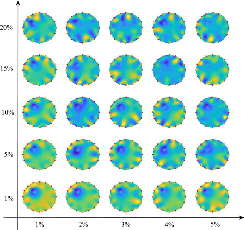
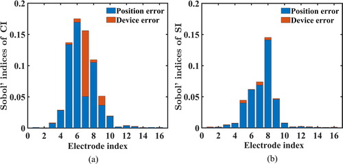
Figure 11 shows the results of the cGSA of the shape detection indices based on the Sobol' indices. As expected, the ci and si sensitivity to the position and device errors indicates that the errors having the most influence on the detection indices were found at electrodes close to the anomaly. Precisely, the device error at the 7th electrode, which was closest to the anomaly, had the greatest influence on ci. Furthermore, most device errors had lesser influence on ci and si than the position errors. However, the position errors at the 8th and 6th electrodes had the greatest influence on ci and si, respectively. Overall, the total contributions of the position and device errors to the detection index variations show that the errors at the electrodes closer to the anomaly had greater influence on the EIT reconstruction.

Figure 11. Results of cGSA for shape detection indices in the case with single anomaly in circular domain: (a) CI and (b) SI. Note that the height of each bar is the sum of the Sobol' indices of the position and device errors.

4.2.2. Two anomalies in body-like domain

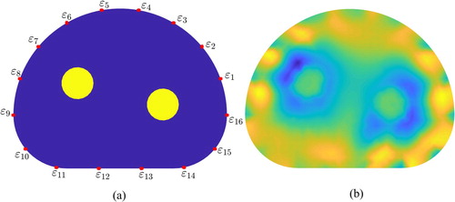
To further validate the proposed framework, we considered a case with two asymmetric anomalies in a body-like domain. Figure 12(a,b) show the domain configuration and the result of reconstruction without measurement errors, respectively. Similar to the circular domain cases, the electrodes were equidistantly distributed along the boundary of the model domain, whereas the two anomalies were asymmetrically placed in the domain. The numerically simulated domain consisted of a noncircular region, as shown in Figure 12, with maximum diameter 2 cm. The electrodes used in this case were still assumed to be points along the computational domain boundary. The conductivity used for the background was 1 S/m, and that for the anomalies was 10 S/m. Although the performance of the inverse solver was poorer than that in the circular domain cases owing to domain complexity, Figure 12(b) confirms that the reconstruction was sufficient to detect the anomalies in the body-like domain.

Figure 12. EIT reconstruction for two circular anomalies in body-like domain: (a) model configuration, and (b) reconstruction without measurement errors.

To perform cGSA, the distributions of the position and device errors were defined as $N(0,{0.03}^2)$ and $N(0,{0.01}^2)$, respectively. Thus, the perturbation percentages of the electrode position and measured potential due to the position and device errors were approximately $10\mathrm{\%}$ and $3\mathrm{\%}$, respectively, which yielded $99.8\mathrm{\%}$ successful reconstructions. Figure 13 shows the results of the cGSA for the ci and si of each anomaly. Similar to the circular domain case in Section 4.2.1, Figure 13(a,c) indicate that the errors having the most influence on the ci variation were associated with the electrodes close to each anomaly. However, the contributions of the position and device errors to the Sobol' indices of ci were comparable, in contrast to the circular domain case. In addition, the device errors at the electrodes neighbouring the electrode closest to each anomaly in this case had greater influence on ci than those in the circular domain case (see Figure 11(a)). Figure 13(b,d) show that the position and device errors at the electrodes close to each anomaly had the most influence on si and that the relative contributions of the device errors to si were negligible, especially for the left anomaly (see Figure 13(b)).

Figure 13. Results of cGSA for shape detection indices in the case with two anomalies in body-like domain: (a) CI and (b) SI of left anomaly, and (c) CI and (d) SI of right anomaly. The electrode index is described in Figure 12(a). Note that the height of each bar is the sum of the Sobol' indices of the position and device errors.

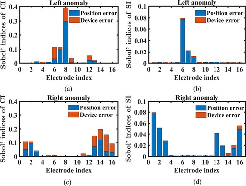
Overall, the EIT reconstruction is more sensitive to the measurement errors at the electrodes close to the target anomaly. This may be related to the asymmetric distributions of the anomalies and the non-circular shape of the domain boundary, which induces more interactive contributions of the measurement errors to the detection indices. The device error contribution to ci becomes significant, whereas si is less sensitive to the device errors.

Finally, we discuss the computation time of ${10}^5$ evaluations of the conductivity fields in cGSA. The Monte Carlo (MC) method for cGSA requires ${10}^5$ simulations to obtain the conductivity fields, which consumes approximately $6.86\times {10}^6$ seconds. However, the PCE method requires only 5000 simulations for all PCE constructions, which consumes approximately $1.41\times {10}^5$ seconds, whereas the cost of ${10}^5$ evaluations of the conductivity fields is negligible. Therefore, the PCE method is approximately 50 times more efficient than the MC method in the evaluation of the conductivity field in cGSA in this example, which demonstrates the efficiency of the proposed framework.

5. Conclusion

In this study, we proposed a framework based on UQ and EIT techniques for quantifying the effect of measurement errors on EIT reconstruction. In this framework, we first introduced two detection indices to evaluate the EIT reconstruction quality. With these detection indices, we selected an appropriate distribution for the measurement error. Then, a sparse PCE surrogate model was constructed for the reconstructed conductivity field. Based on this surrogate model, we investigated the effect of the measurement errors on the detection indices using variance-based global sensitivity analysis. Finally, Sobol' indices were obtained for the detection indices, from which the relative contributions of each measurement error to the uncertainty of the EIT reconstruction could be clearly seen. The performance of the proposed framework was investigated for several EIT problems, i.e. EIT image reconstruction for cases with one or two anomalies in a circular domain, and EIT image reconstruction for the case of two anomalies in a body-like domain. The results show that the errors at the electrodes close to the anomaly had the most influence on the EIT reconstruction uncertainty. Furthermore, when both position and device errors were considered, the contrast index of each anomaly was found to be highly sensitive to all position and device errors at the electrodes close to the anomaly, while the similarity index was only significantly sensitive to the position errors. In summary, the proposed framework is efficient and feasible for application to quantify the effect of measurement errors on EIT reconstruction. As a next step, more generic cases (e.g. object with non-circular inclusions) are needed to fully validate the proposed framework. Furthermore, we intend to develop a framework combining the current framework with reduced-order modelling techniques to address the case requiring very high discretization resolution in the computational domain.

Disclosure statement

No potential conflict of interest was reported by the author(s).

Additional information

Funding

This work was supported by the National Research Foundation of Korea (NRF) grant funded by the Korea government (Ministry of Science and ICT) (NRF-2017R1E1A1A0-3070161 and NRF-20151009350).

References

- Kolehmainen V, Vauhkonen M, Karjalainen PA, Kaipio JP. Assessment of errors in static electrical impedance tomography with adjacent and trigonometric current patterns. Physiol Meas. 1997;18(4):289–303.
- Borcea L. Electrical impedance tomography. Inverse Probl. 2002;18(6):99–136.
- Holder D. Electrical impedance tomography: methods, history and applications. Boka Raton: CRC Press; 2004.
- Seo JK, Woo EJ. Nonlinear inverse problems in imaging. West Sussex: John Wiley & Sons; 2012.
- Vauhkonen M, Vadasz D, Karjalainen PA, Somersalo E, Kaipio JP. Tikhonov regularization and prior information in electrical impedance tomography. IEEE Trans Med Imag. 1998;17(2):285–293.
- Borsic A Regularization methods for imaging from electrical measurements [Ph.D thesis]. Oxford Brookes University; 2002.
- Karageorghis A, Lesnic D. The method of fundamental solutions for the inverse conductivity problem. Inverse Probl Sci Eng. 2010;18(4):567–583.
- Lee K, Woo EJ, Seo JK. A fidelity-embedded regularization method for robust electrical impedance tomography. IEEE Trans Med Imag. 2017;37(9):1970–1977.
- Nissinen A, Kolehmainen V, Kaipio JP. Reconstruction of domain boundary and conductivity in electrical impedance tomography using the approximation error approach. Int J Uncertain Quan. 2011;1(3):203–222.
- Dardé J, Hyvönen N, Seppänen A, Staboulis S. Simultaneous reconstruction of outer boundary shape and admittivity distribution in electrical impedance tomography. SIAM J Imaging Sci. 2013;6(1):176–198.
- Bardsley JM, Seppänen A, Solonen A, Haario H, Kaipio J. Randomize-then-optimize for sampling and uncertainty quantification in electrical impedance tomography. SIAM/ASA J Uncertain Quan. 2015;3(1):1136–1158.
- Hyvönen N, Leinonen M. Stochastic Galerkin finite element method with local conductivity basis for electrical impedance tomography. SIAM/ASA J Uncertain Quan. 2015;3(1):998–1019.
- Hyvönen N, Kaarnioja V, Mustonen L, Staboulis S. Polynomial collocation for handling an inaccurately known measurement configuration in electrical impedance tomography. SIAM J Appl Math. 2017;77(1):202–223.
- Ren S, Soleimani M, Xu Y, Dong F. Inclusion boundary reconstruction and sensitivity analysis in electrical impedance tomography. Inverse Probl Sci Eng. 2018;26(7):1037–1061.
- Adler A. Accounting for erroneous electrode data in electrical impedance tomography. Physiol Meas. 2004;25(1):227–238.
- Meeson S, Blott BH, Killingback AL. EIT data noise evaluation in the clinical environment. Physiol Meas. 1996;17(4A):33–38.
- Frangi AR, Riu PJ, Rosell J, Viergever MA. Propagation of measurement noise through backprojection reconstruction in electrical impedance tomography. IEEE Trans Med Imag. 2002;21(6):566–578.
- Seo JK, Woo EJ. Electrical tissue property imaging at low frequency using MREIT. IEEE Trans Biomed Eng. 2014;61(5):1390–1399.
- Al-Hatib F. Patient-instrument connection errors in bioelectrical impedance measurement. Physiol Meas. 1998;19(2):285–296.
- Lozano A, Rosell J, Pallás-Areny R. Errors in prolonged electrical impedance measurements due to electrode repositioning and postural changes. Physiol Meas. 1995;16(2):121–130.
- Dardé J, Hakula H, Hyvönen N, Staboulis S, Somersalo E. Fine-tuning electrode information in electrical impedance tomography. Inverse Probl Imag. 2012;6(3):399–421.
- Dardé J, Hyvönen N, Seppänen A, Staboulis S. Simultaneous recovery of admittivity and body shape in electrical impedance tomography: an experimental evaluation. Inverse Probl. 2013;29(8):085004.
- Kourunen J, Savolainen T, Lehikoinen A, Vauhkonen M, Heikkinen LM. Suitability of a PXI platform for an electrical impedance tomography system. Meas Sci Technol. 2008;20(1):015503.
- Lieberman C, Willcox K, Ghattas O. Parameter and state model reduction for large-scale statistical inverse problems. SIAM J Sci Comput. 2010;32(5):2523–2542.
- Gehre M, Jin B. Expectation propagation for nonlinear inverse problems–with an application to electrical impedance tomography. J Comput Phys. 2014;259:513–535.
- Leinonen M, Hakula H, Hyvönen N. Application of stochastic Galerkin FEM to the complete electrode model of electrical impedance tomography. J Comput Phys. 2014;269:181–200.
- Adler A, Guardo R. Electrical impedance tomography: regularized imaging and contrast detection. IEEE Trans Med Imag. 1996;15(2):170–179.
- Smith RC. Uncertainty quantification: theory, implementation, and applications. Philadelphia: SIAM; 2013.
- Ghanem RG, Spanos PD. Stochastic finite elements: a spectral approach. New York: Courier Corporation; 2003.
- Xiu D, Karniadakis GE. The Wiener–Askey polynomial chaos for stochastic differential equations. SIAM J Sci Comput. 2002;24(2):619–644.
- Babuška I, Nobile F, Tempone R. A stochastic collocation method for elliptic partial differential equations with random input data. SIAM Rev. 2010;52:317–355.
- Kucherenko S, Klymenko OV, Shah N. Sobol' indices for problems defined in non-rectangular domains. Reliab Eng Syst Saf. 2017;167:218–231.
- Cheng KS, Isaacson D, Newell JC, Gisser DG. Electrode models for electric current computed tomography. IEEE Trans Biomed Eng. 1989;36(9):918–924.
- Somersalo E, Cheney M, Isaacson D. Existence and uniqueness for electrode models for electric current computed tomography. SIAM J Appl Math. 1992;52(4):1023–1040.
- Cheney M, Isaacson D, Newell JC. Electrical impedance tomography. SIAM Rev. 1999;41(1):85–101.
- Tikhonov A, Arsenin V. Solutions of iIll-posed problems. New York: Winston; 1977.
- Hua P, Woo EJ, Webster JG, Tompkins WJ. Iterative reconstruction methods using regularization and optimal current patterns in electrical impedance tomography. IEEE Trans Med Imag. 1991;10(4):621–628.
- Hua P, Webster JG, Tompkins WJ. A regularised electrical impedance tomography reconstruction algorithm. Clin Phys Physiol Meas. 1988;9(4):137–141.
- Cheney M, Isaacson D, Newell JC, Simske S, Goble J. NOSER: an algorithm for solving the inverse conductivity problem. Int J Imag Syst Technol. 1990;2(2):66–75.
- Kim S, Lee EJ, Woo EJ, Seo JK. Asymptotic analysis of the membrane structure to sensitivity of frequency-difference electrical impedance tomography. Inverse Probl. 2012;28(7):075004.
- Zhang T, Lee E, Seo JK. Anomaly depth detection in trans-admittance mammography: a formula independent of anomaly size or admittivity contrast. Inverse Probl. 2014;30(4):045003.
- Zhou W, Bovik AC, Sheikh HR, Simoncelli EP. Image qualifty assessment: from error visibility to structural similarity. IEEE Trans Image Process. 2004;13(4):600–612.
- Walters R Towards stochastic fluid mechanics via polynomial chaos. In: 41st AIAA aerospace sciences meeting & exhibit. Reno, NV; 2003.
- Hosder S, Walters R, Balch M Efficient sampling for non-intrusive polynomial chaos applications with multiple uncertain input variables. In 48th AIAA/ASME/ASCE/AHS/ASC structures, structural dynamics, and materials conference; 2007. p. 1939.
- Blatman G, Sudret B. Adaptive sparse polynomial chaos expansion based on least angle regression. J Comput Phys. 2011;230(6):2345–2367.
- Efron B, Hastie T, Johnstone I, Tibshirani R. Least angle regression. Ann Stat. 2004;32(2):407–499.
- Helton JC, Davis FJ. Latin hypercube sampling and the propagation of uncertainty in analyses of complex systems. Reliab Eng Syst Saf. 2003;81(1):23–69.
- Sobol IM. Sensitivity estimates for nonlinear mathematical models. Math Model Comput Exp. 1995;1(4):407–414.
- Sudret B. Global sensitivity analysis using polynomial chaos expansions. Reliab Eng Syst Saf. 2008;93(7):964–979.
- Crestaux T, Le Maître O, Martinez JM. Polynomial chaos expansion for sensitivity analysis. Reliab Eng Syst Saf. 2009;94(7):1161–1172.
- Ghaffari S, Magin T, Iaccarino G Uncertainty quantification of radiative heat flux modelling for Titan atmospheric entry. In: 48th AIAA aerospace sciences meeting including the new horizons forum and aerospace exposition; 2010. p. 239.
- Fisher RA. Statistical methods for research workers. Edinburgh: Genesis Publishing Pvt Ltd; 1925.