Differentiation of materials and laser powder bed fusion processing regimes from airborne acoustic emission combined with machine learning

ABSTRACT

This study investigates the use of a low cost microphone combined with state-of-the-art machine learning (ML) algorithms as online process monitoring to differentiate various materials and process regimes of Laser-Powder Bed Fusion (LPBF). Three processing regimes (lack of fusion pores, conduction mode and keyhole pores) and three alloys (316L stainless steel, bronze (CuSn₈), and Inconel 718) were selected. Three conventional ML algorithms and a Convolutional Neural Network (CNN) were chosen to perform the classification tasks resulting in five main findings. First, we proved that the AE features are related to the laser-material interaction and not from undesired machine or environmental noise. Second, the process regimes are classified with high accuracy (> 87%) regardless of the algorithms and materials. Third, it is possible to build a single model from the three materials and still reach high classification accuracy (>86%) of the different regimes. Forth, the AE features used for the classifications are material and regime dependent. Finally, with LPBF processing of multi-materials on the rise, a strategy for classifying the material and the process regimes simultaneously using a CNN multi-label architecture reached a very high classification accuracy (≈ 93%). The results demonstrate the potential of our approaches for online LPBF process monitoring of different materials and regimes.

KEYWORDS:

• Acoustic emission
• additive manufacturing
• in situ monitoring
• machine learning
• artificial intelligence
• laser material processing

1. Introduction

Laser-Powder Bed Fusion (LPBF) is the most studied laser-based three-dimensional (3D) printing process, which consolidates parts, layer-by-layer, from powders (King et al. 2015). Metallic 3D printed workpieces via LPBF can achieve near full-density, and the resulting mechanical properties are comparable with (or even exceed) those obtained by conventional processing routes (Yap et al. 2015; DebRoy et al. 2018). Though the process looks conceptually simple, the underlying dynamics of rapid melting and cooling of the melt pool, the powder stock material properties, and the surrounding environments make it complicated and prone to defects such as balling, LoF pores, and keyhole pores. The formation of such defects limits technology applications (King et al. 2015; Dowling et al. 2020; Khairallah et al. 2016; du Plessis, Yadroitsava, and Yadroitsev 2020).

It is well known that the quality of the produced part during LPBF is directly dependent on the process window parameters such as laser energy density, the composition of the powder alloy, scanning speed, layer thickness, strategy for scanning, environment, etc. (Chua, Ahn, and Moon 2017; Van Elsen 2007; Spears and Gold 2016; Gu et al. 2006; Kurzynowski et al. 2012). The range of process parameters to achieve near full-density characteristics is limited to a narrow window, called the keyhole threshold (Qi et al. 2017; King et al. 2014; Cunningham et al. 2019; Ghasemi-Tabasi et al. 2020). Identifying the optimal processing window is tremendously time-consuming and expensive as it requires a trial and error approach (Aboulkhair et al. 2014), sometimes coupled with numerical simulations (King et al. 2015; Heeling, Cloots, and Wegener 2017; Mukherjee and DebRoy 2018). During the LPBF process, lack of energy input causes incomplete overlap of the melt pool with the adjacent layer resulting in porosity formation called Lack of Fusion (LoF) pores (Gong et al. 2014). LoF pores appear in two forms: weak bonding or incompletely melted metal particles (Zhang, Li, and Bai 2017). LoF pores are irregularly shaped and can be larger than 500 μm, resulting in an epicentre of crack propagation during cyclic loading when the part is operational (Coeck et al. 2019). An increase in energy density produces melt pools with shallow depths known as conduction mode, where the ratio between the melting depth (D) and laser beam diameter (Ø_laser) is D/Ø_laser ≤ 1. In LPBF, the conduction mode refers to processing conditions with a density higher than 99.9%. A further increase in energy density leads to deeper melt pools depths, eventually resulting in the intense evaporation of the material, which causes the formation of a vapour channel called a keyhole. The stability of the keyhole mechanism is known to be rather unstable (Le-Quang et al. 2018). Its collapse during the process leaves behind trails of voids (King et al. 2014). Actually, this porosity occurs mainly when the volumetric energy density is too high; such pores are called keyhole pores (Thanki et al. 2019). Apart from porosities occurring due to suboptimal laser parameters, porosities can also occur based on the powder composition's physical property. Indeed, the physical property of the powder alloys influences heat absorption and heat transfer during the process. The high solidification rate traps the gas bubbles before it rises and escapes, resulting in defect inclusions in the shape of spherical pores (Zhang, Li, and Bai 2017). Even when the parameters have been well defined, the defect formation due to laser-material interaction is known to be highly non-linear and stochastic by nature, making it significantly non-reproducible (Dowling et al. 2020; du Plessis, Yadroitsava, and Yadroitsev 2020; Nassar et al. 2019). One solution to this drawback is developing an in situ and real-time process regime monitoring technique; the main aim of this contribution. Monitoring the process and interpretation of the sensor data helps to understand and mitigate the many unfavourable events happening in the process zone (Shevchik et al. 2018; Everton et al. 2016).

In recent years, process monitoring and control of metal-based LPBF processes have been the main focus of several investigations. It helps in a broader adaptation as a mainstream manufacturing technique in industries (Masinelli et al. 2020). Based on the reviews of Tapia and Elvany (Tapia and Elwany 2014), Everton et al. (Everton et al. 2016), Grasso and Colosimo (Grasso et al. 2018), and Yan et al.(Yan et al. 2018), the most popular monitoring method is by in situ optical inspections of the process zone using photodiodes and high-speed cameras. For the former method, which also includes pyrometers, the optical radiations emitted and reflected from the process zone are sensed by photodiodes. Information regarding the temperature, laser energy coupling inside the workpiece, and process stability can be derived using photodiodes (Shevchik et al. 2020; Shevchik et al. 2019; Forien et al. 2020; Yan et al. 2018). The advantage of this method is that it is cost-efficient and has outstanding temporal resolutions. Commercial photodiodes detect bandwidths of several megahertz up to gigahertz, making them capable of following highly dynamic processes such as laser-material interaction (Le-Quang et al. 2018; Zhao et al. 2017). Nevertheless, as the signals are averaged over the photodiode field-of-view, this method lacks spatial resolution. The use of high-speed cameras can overcome this issue. With a suitable camera and optical setup, information regarding the melt pool's geometry, temperature distribution on the workpiece's surface, evolution and fluctuation of the vapour plume, and even the ejections of liquid droplets (spatters) can be obtained (Grasso et al. 2018; Hooper 2018; Yan et al. 2018). High-speed cameras are significantly advantageous for the physical understanding of the process. However, its industrial implementation for process monitoring suffers from the very high cost of the system. Another common disadvantage of optical detection methods is that they are limited to the process zone's surface region. Consequently, the detection of defects, such as porosity and cracks, is challenging. An alternative to optical methods is the acoustic emission (AE) technique. Acoustic sensors can detect sound waves generated by an additive manufacturing machine. It includes the laser-material interaction, propagating inside the workpiece (structure-borne) and atmosphere (airborne). Therefore, they are very sensitive to the process zone's volumetric behaviours and can detect better the process instabilities that lead to porosity and cracks (Shevchik et al. 2020; Shevchik et al. 2019; Shevchik et al. 2018; Shevchik et al. 2019). Obviously, the origin of AE source in metal-based LPBF processes are manifolds such as laser-material interaction (rapid melting and cooling, defect formation and related process regime) as well as undesired environment and machine noises and finally even from the process parameters themselves. Like photodiodes, acoustic sensors are also cost-efficient and have been successfully implemented to monitor other industrial dynamic processes (Pandiyan et al. 2020; Pandiyan and Tjahjowidodo 2019, 2017). The AE combined with machine learning methods has a proven track record in carrying information of the process zone when a thermal source (Chen, Kovacevic, and Jandgric 2003; Wu, Wang, and Yu 2016; Wu, Yu, and Wang 2017) or laser (Gu and Duley 1996; Wasmer et al. 2018; Shevchik et al. 2019) interacts with a material.

The accomplishment of real-time monitoring in any dynamic process requires the computers to learn and model the patterns in the sensor data. The perspectives of using Machine Learning (ML) in metal-based LPBF has been written by Sing et al. (Sing et al. 2021) and the one in 3D bioprinting by Yu and Jiang (Yu and Jiang 2020). Scime and Beuth (Scime and Beuth 2018a, 2018b, 2019; Scime et al. 2020) published several approaches using cameras and Machine Learning (ML) to identify process footprints leading to defect creation. They used computer vision algorithms (Scime and Beuth 2018a) and Convolutional Neural Network (CNN) (Scime and Beuth 2018b) during the powder spreading stage of the process to detect and classify anomalies automatically. They used a similar approach (computer vision algorithms) and unsupervised ML to differentiate between observed melt pools Scime and Beuth (2019). Digital camera images were combined with a deep residual neural network and region proposal network to detect the powder bed defects, namely, the warpage, part shifting, and short feed (Xiao, Lu, and Huang 2020). Alessandra Caggiano et al. (Caggiano et al. 2019) have combined the powder bed and process zone images with a Bi-stream CNN to detect the process quality. Apart from optical methods, thermal sensor data have been used along with ML algorithms such as K-Nearest Neighbour (KNN) and Decision Tree (DT) to predict part quality (Khanzadeh et al. 2018). Khanzadeh et al. (Khanzadeh et al. 2018) have also proposed a multilinear principal component analysis (MPCA) approach for extraction of low dimensional features from thermal maps to monitor AM process. In the literature, AE has been combined with Spectral CNN (Shevchik et al. 2018; Shevchik et al. 2019; Wasmer et al. 2018), deep belief networks (Ye et al. 2018), reinforcement learning (Wasmer et al. 2019), and Support Vector Machine (SVM) (Ye et al. 2018) for real-time monitoring of the LPBF processes, but always for a single material and one process condition per regime. In recent years, in addition to online monitoring, ML algorithms have been either applied in other fields of AM such as developing process model or are combined with physics based-models such as Finite Element (FE) simulations to overcome the problem of data-driven approach. Jiang et al. (Jiang et al. 2020) exploited deep neural networks to predict the connection status between printed lines taking into account four process parameters; filament extrusion speed, print speed, line distance and layer height. Ren et al. (Ren et al. 2021) published a work where they used a Temperature-Pattern Recurrent Neural Networks (TP-RNN) model to predict the temperature field for multi-layer cube deposition planning. Finally, a comprehensive review of ML algorithms used in the context of additive manufacturing has been reported by Goh et al. (Goh, Sing, and Yeong 2021).

While literature reports monitoring the LPBF process dealing with one material, artificial intelligence (AI) techniques in monitoring different materials are seldom mentioned. When analysing AE signals with ML, the identification of different types of porosities in 316L stainless steel was demonstrated successfully (Shevchik et al. 2019; Shevchik et al. 2018). Moving to another material or generalisation among materials would require the building of a new database, which leads to the following questions:

1. Are the acoustic signatures material dependent, or instead, can it be generalised for broader scenarios? In other words, a distinct database for materials having different mechanical, optical and thermal properties are needed, or can a single database be used? This question was not examined so far in the literature.

2. Can a single ML model monitor the process regimes when dealing with different materials be built if the acoustic signatures are material-dependent?

3. Can we distinguish both the material and the regime when dealing with different materials? If so, it would provide precious information on the material(s) in which defects are formed without the need for time-consuming microscopy analysis.

The reported work investigates the AE features recorded during LPBF, resolved in time, frequency, and time–frequency domains, and statistically correlates them with the occurrence of three process regimes: LoF pores, keyhole pores, or with the absence of pores (conduction mode). As mentioned earlier, the conduction mode refers to processing conditions with a density higher than 99.9%. The analysis is performed on three different material alloys, stainless steel (316L), bronze (CuSn₈), and Inconel (Inconel 718), that have distinct optical, mechanical and thermal properties. Four ML models based on Logistic regression (LR), Random Forest (RF), Support Vector Machines (SVM), and a CNN were selected for classification tasks of the process regimes. The rising attention for producing different materials part using the LPBF techniques brings new process monitoring challenges. To address them, a new approach by developing a CNN architecture able to classify the process regimes and the processed alloy is proposed. The ability to analyse AE features of different alloys provides key information for answering questions (i) and (ii) related to the generalisation of ML algorithms and to the possibility of distinguishing the different alloys using a single model. Finally, a CNN-based multi-label classification model addresses question (iii) on distinguishing regimes and materials.

The paper is organised into 6 Sections. Experimental considerations are presented in Section 2. The analysis of the acoustic signal emitted during the LPBF process in time, frequency, and time–frequency domains for the three alloys is summarised in Section 3. The representations and visualisation of the acoustic features in low dimensional space using t-distributed Stochastic Neighbour Embedding (t-SNE) is discussed in Section 4. Section 5 starts by determining the origin of AE features used for classification. Then, it presents the results of the developed online monitoring systems for the different materials and process regimes using traditional ML and CNN architectures; focusing on the universality and material identification aspects. Finally, this paper's findings and future works on in situ and real-time monitoring for the LPBF process are discussed in Section 6.

2. Experimental setup and data acquisition

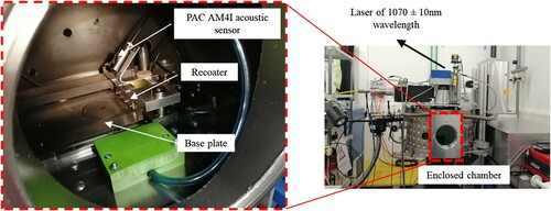
In this work, the experiments were performed on an in-house LPBF system shown in Figure 1. The customised LPBF system can have a scan speed up to 20 m·s⁻¹. The enclosed chamber of the LPBF system has a Continuous-Wave (CW) modulated Ytterbium fibre laser for melting the powder and a recoater mechanism for creating a new powder layer. The fibre laser operates in continuous mode with a 1070 ± 10 nm wavelength, and the beam is around 82 microns (1/e²) at the focal plane with an M² < 1.1. The recoater mechanism spreads the metal powder to a thickness of around 40 μm. The chamber's atmosphere is controlled under a laminar flowing closed loop of argon and a monitored maximum oxygen level of 200 ppm. The LPBF system is equipped with a PAC AM4I (Physical Instrument, Germany) airborne acoustic sensor, hereafter referred to as microphone, and an Advantech Data Acquisition (DAQ) card (Advantech, Taiwan) to get feedback from the process zone.

Figure 1. Experimental setup of the LPBF process with the PAC AM41 acoustic sensor installed.

All experiments were performed with the in-house LPBF system. To start with, we built some transition layers of a selected material on the base plate. These transition layers have two main purposes. First, it will act as a transition material from the base plate to the one processed. Second, it must be thick enough to ensure that our experiments will have the same heat flow as processing a single material. As these transition layers do not require to be of high quality, faster processing parameters were selected layers to save preparation time. On top of these transition layers, high-density layers were built to guarantee the same initial condition for the experiments with chosen proves parameters. Finally, a series of overlapping line tracks were produced during which the AE signals were recorded with the PAC AM4I microphone. The transition layers, the high-density layers and the overlapping line tracks can be seen in Figure 4. To simplify the design space, the scanning strategy selected is one-directional and parallel, with a hatch distance of 0.1 mm. The experiments were performed with three different alloys, stainless steel (316L), bronze (CuSn₈) and Inconel (Inconel 718), and their corresponding chemical composition are summarised in Table 1. The Stainless Steel 316L micro powder, MetcoAdd 316L, was bought from Oerlikon Metco with a particle size distribution between 45 and 15 µm. The bronze (CuSn₈) powder having an average particle size of 30 µm was purchased from Heraeus Materials SA. The nickel-based super-alloy Inconel 718 powder was purchased from Oerlikon Metco, exhibiting a bimodal particle size distribution with peak values at 45 and 15 µm.

Table 1. Chemical composition of the powders of Nickel-based super-alloy (Inconel 718)), bronze (CuSn₈), and stainless steel (316L).

Chemical composition of stainless steel (316L) powder
Fe	Cr	Ni	Mo	Other	C
Balance	18	12	2	< 1.00	< 0.03
Chemical composition of Bronze (CuSn8) powder
Cu	P	S	Fe	Ni	Zn	As	Zr
Balance	0.06 ± 0.02	≤ 0.05	≤ 0.05	< 0.03	≤ 0.2	≤ 0.05	≤ 0.05
Chemical composition of Inconel (718) powder
Ni	Fe	Cr	Nb + Ta	Mo	Ti	Al	Other
Balance	18	18	5	3	1	0.60	< 0.5

The microphone was positioned at a distance of approximately 10 cm from the build plate, as shown in Figure 1. It has a frequency response in the range of 0–100 kHz. The AE signals were acquired at a rate of 1 MHz and stored locally for further processing with a custom-built C# code runs on a PC which can interact with the Advantech DAQ card. The data acquisition rate was chosen to ensure that the Nyquist Shannon theorem (Jerri 1977) is satisfied. The captured signal was triggered by a photodiode using a beam splitter setup. This configuration ensures that the process and the data obtained are synchronised. Once the laser interacts with the powder bed, the photodiode's minimum amplitude threshold is surpassed, which triggers the acquisition of the acoustic signals and the data recording. Prior to analysing the signal features in time, frequency, and time–frequency domains, they were filtered with a low-pass Butterworth filter to remove frequency contents higher than 100 kHz as they do not fall inside the sensitivity range of the AE sensor.

In this contribution, the three most common process regimes known in LPBF are investigated; they are LoF pores, conduction mode (or absence of pores), and keyhole pores (Qi et al. 2017; King et al. 2014; Cunningham et al. 2019; Ghasemi-Tabasi et al. 2020). The conduction mode regime is considered the normal regime since it results in the highest material density in conjunction with adequate material properties. In contrast, LoF pores and keyhole pores are considered as abnormal regimes and must be avoided. In addition, two process parameters were selected per regime. The reasons lying behind the selection of process regimes and parameters are fourfold. First, selecting two sets of parameters for each regime was motivated by the fact that, in the literature, most studies used a single process parameter per regime, such as in Shevchik et al. (Shevchik et al. 2018), and this limits the sampling of the process space. Adding a second process parameter for each regime will give a finer representation of the process space and demonstrate that our approach is valid for multi-process parameters. Second, to ensure that AE features selected for the classification task are solely related to the process regimes and not from the undesired environment, the machine noises, or machine parameters; one set of laser parameters (bold red values in Table 2) were identical for all three alloys for the regimes, LoF pores and keyhole pores. Having the same process parameter for a specific regime across the material guarantees that the undesired environment, the machine noises, and the machine parameters are identical. Hence, under such circumstances, being able to differentiate the material will prove that AE features are exclusively correlated to the laser-material interaction and so the process regime. Third, rather than selecting the second set of parameters randomly within both regimes, it was decided to have them based on a physical basis. Consequently, they were chosen to have the same normalised enthalpy (Qi et al. 2017; King et al. 2014; Cunningham et al. 2019; Ghasemi-Tabasi et al. 2020) across all alloys (blue values in Table 2 and also shown in Figure 2). Finally, as it is not possible to achieve the regime conduction mode with the same laser parameters sets due to the differences in material properties, we selected the process parameters having a normalised enthalpy around 25, which was proven to be an optimised value for high-density conduction mode in three materials, including 316L stainless steel and bronze (Ghasemi-Tabasi et al. 2020) (green values in Table 2, and circled points in Figure 2). Based on these considerations, the selected laser parameters for inducing or avoiding defects are listed in Table 2 for the three selected alloys. A total of 100 line track experiments were performed for each set of process parameters on each alloy. The analysis of the corresponding acoustic signatures is reviewed in Section 3.

Figure 2. Processing map showing the normalised melt pool depth (i.e. depth divided by the laser spot size) as a function of the normalised enthalpy (as defined in (Ghasemi-Tabasi et al. 2020)) for the printed stainless steel, Inconel and bronze samples. The optimal processing condition is around a normalised enthalpy of 25 for all alloys (Ghasemi-Tabasi et al. 2020). Lower normalised enthalpies lead to LoF pores, while larger values lead to keyhole pores. Experimental setup of the LPBF process with the PAC AM41 acoustic sensor installed.

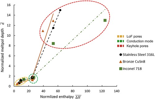
Table 2. Two set of laser parameters for stainless steel, bronze and Inconel to induce the process regimes (regimes) LoF pores, conduction mode and keyhole pores. In bold, the first set of parameters for LoF pores, and keyhole pores is kept constant for the three alloys.

Regimes	Stainless steel			Bronze			Inconel
	Laser power (W)	Scan speed (mm/s)	Normalized enthalpy	Laser power (W)	Scan speed (mm/s)	Normalized enthalpy	Laser power (W)	Scan speed (mm/s)	Normalized enthalpy
LoF pores	50	350	7	50	350	4.4	50	350	13.4
	70	400	9.2	110	400	9.2	36	400	9.2
Conduction mode	180	350	25	300	350	26.5	100	350	27
	135	200	25	215	200	25	69	200	25
Keyhole pores	450	350	63	450	350	39.4	450	350	124
	250	150	53.5	396	150	53.5	127	150	53.5

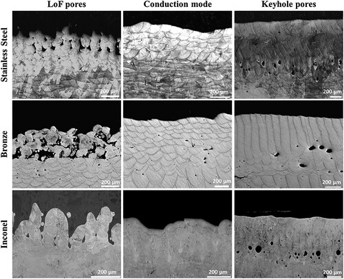
The diagnostic on the type of defect regimes (regime) for data labelling was obtained and confirmed via X-ray tomography (Figure 3) and cross-sectioning of selected lines (Figure 4). Based on this analysis and experience, the same process regime was assumed for each of the 100 lines using the same process parameters. Typical micrographs, representative of the three labelled regimes for the three materials, are shown in Figure 4. In this figure, the three process zones are visible. At the bottom of the figure, the preparation cube is characterised by a large melt zone and high defect content. It is followed by a high-density layer, which for the conduction mode are identical to the top layer. The latter is made of overlapping line tracks during which the AE signals are recorded. The samples were etched to reveal the melt pools, whose depths are reported in Figure 2. The stainless steel, bronze and Inconel samples were etched with (i) Aqua regia diluted (100 mL HNO₃,100 mL HCl,100 mL H₂O) for 30 s, (ii) ASTM No.30 (5 mL H2O2, 25 mL NH3, 25 mL H2O) for 5–10 s, and (iii) Kalling’s No.2 Reagent (5 g CuCl, HCl 100 mL, C2H6O 100 mL, H2O 100 mL) for 10–20 s, respectively. Micrographs were taken with a Leica DM6000M light optical microscope in bright field mode.

Figure 3. Keyhole porosity formation along one laser track, in stainless steel (316L), and its corresponding acoustic emission signal; (a) 3D reconstruction of the keyhole pores formed in one line; (b) 2D section of region shown in (a); (c) acoustic emission signal corresponding to the selected laser track.

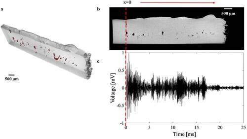
Figure 4. Typical micrographs of the three regimes (LoF pores, conduction mode and keyhole pores) for stainless steel (316L), bronze (CuSn₈), and Inconel (Inconel 718).

3. Analysis of acoustic emission signature from LPBF process

As already mentioned, the LPBF process suffers from a lack of repeatability due to defect formation's stochastic nature. This inconvenience results in the occurrence of defects such as LoF pores and keyhole pores. For real-time identification of these defects, it is imperative to have information about the changes taking place in the process zone over time. In Pandiyan et al. (Pandiyan et al. 2020), such analysis was performed for 316L for the three regimes investigated in this study, along with balling (another type of lack-of-fusion mechanism). The study's outcomes proved features in time, frequency, and time–frequency domains are specific for different regimes. A similar analysis on the three selected alloys is performed to determine whether the conclusion can be generalised for other alloys too. Besides, we will investigate whether the features in the three domains are specific to each alloy. To perform the feature analysis, similar to Pandiyan et al. (Pandiyan et al. 2020), a window of 5 ms is used to split the sensor's signals to extract several features in the three domains. It was selected after an exhaustive search to reach the best compromise between time resolution and classification accuracy. A short running window increases defect detection time and spatial resolution but are also sensitive to limited information and noise. The period must be minimum enough to cover a defect formed with the chosen parameters. The choice of the window size for features analysis is the same as the one chosen for the classification which will be discussed later.

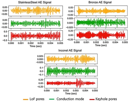
Figure 5 compares typical raw AE signals (peak-to-peak) corresponding to the three regimes from the three alloys. Specifically, it indicates that irrespective of the alloy, the AE signals’ amplitude increases from LoF pores to keyhole pores.

Figure 5. Raw AE signals correspond to the three different regimes: LoF pores, conduction mode, and keyhole pores for stainless steel, bronze and Inconel (Note: Signal corresponding to LoF pores and keyhole pores regimes for the three alloys are using same process parameter).

3.1. Time-domain analysis

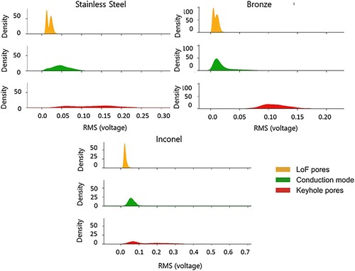
The time-domain analysis gives the features as a function of amplitude changing over time. The statistical distribution of the features based on time-domain such as Root Mean Square (AE_RMS), mean, crest-power, standard deviation, skewness, variance, kurtosis, median, etc., were analysed to correlate with the three selected regimes. As the conclusions are similar for all features distributions, only the AE_RMS distribution for the three regimes in the three alloys is shown in the form of a ridge plot in Figure 6. The range of AE_RMS distribution values in LoF pores for stainless steel and Inconel are higher less than for bronze. This may be related to the absorptivity at the laser Near-Infrared Red (NIR) wavelength, lower in bronze than the two other alloys. Therefore, the required input energy to reach the conduction mode for the bronze alloy needs to be higher, even though the bronze melting point is lower (Ghasemi-Tabasi et al. 2020). The distribution of AE_RMS starts to spread as the regime moves from LoF pores to conduction mode, while keyhole pores have a much larger deviation. This may be due to the highly unstable behaviour of the keyhole (Shevchik et al. 2020). The examination of time-domain features such as skewness, crest-power, median, kurtosis, etc., also exhibited distinct distributions amongst the regimes for all three alloys. Such a distinct distribution of statistical time-domain features motivates the use of ML algorithms to perform real-time monitoring.

Figure 6. Distribution of AE_RMS features for the three regimes occurring in stainless steel, bronze and Inconel.

3.2. Frequency domain analysis

The periodic components of a signal can be identified when the signal is resolved in the frequency domain. To be specific, decomposing a signal with Fast Fourier Transforms (FFT) analysis reveals these periodic components’. The representation of AE in the frequency domain for all three regimes provided additional interesting insights compared to the time domain. Figure 7 presents the Power Spectral Density (PSD) distribution in the FFT plots, which was calculated using the Welch method (Welch 1967) for a window of 5 ms. Irrespective of the alloys, distinct peaks are visible at more or less 10 and 40 kHz, as evident from Figure 7 across the three regimes. Most peaks were found around these frequency bands, as the PAC AM4I acoustic sensor's response was also higher in this region. Besides, for the regime keyhole porosity of bronze, it can be inferred that the magnitude of the frequency content in the vicinity of 10 kHz is higher than at 40 kHz.

Figure 7. Typical FFT plots for stainless steel, bronze and Inconel depicting discrete frequency distributions among the alloys and across the three regimes.

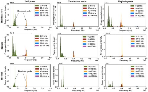
In contrast, the PSD distribution values corresponding to LoF pores were much lower than for other alloys for bronze. This decrease may again be related to the lower absorptivity of bronze at the NIR wavelength. When processing Inconel, the frequency peaks were found at more or less 10 and 40 kHz for all regimes except for the conduction mode. For Inconel, a surge in frequency peaks around 10 kHz compared to other frequency ranges seems to be correlated to a high-density conduction mode process. It is also to be noted that regimes across alloys showed some degree of resemblance, for example, as indicated by arrows in Figure 7 on LoF pores between stainless steel and Inconel.

One of the most critical aspects of the frequency domain analysis is understanding the correlation between signal power densities in different frequency bands for each regime. The microphone's operating range of 1–100 kHz was divided into five frequency bands, namely 0–20 kHz, 20–40 kHz, 40–60 kHz, 60–80 kHz, and 80–100 kHz for such an analysis. All results, in terms of cumulative energy density values for a window size of 5 ms calculated by the periodogram method (Babtlett 1948), are presented in Figure 8. This figure is important since the energy density distribution plots between the five bands were calculated on the whole dataset. Therefore, it gives an overall sparse representation between the alloys and regimes. For bronze, stainless steel, and Inconel, the energy contents were concentrated within the frequency range of 0–60 kHz.

Figure 8. Comparison of cumulative energy content between five frequency bands for three regimes in stainless steel, bronze and Inconel.

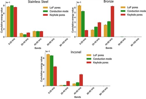
In contrast, the frequency bands below 40 kHz have more significant contributions for stainless steel, especially in the conduction mode. As shown in Figure 8, the energy level concentration of the regimes LoF pores was prevalent in the frequency band of 0–20 kHz for all alloys. However, for the regime conduction mode of Inconel (Figure 8 (a)), there is a decrease in the energy density value of the frequency band 40–60 kHz as compared to the other alloys. From the energy density distribution plots, it can be concluded that laser interaction with the molten pool causes AE signals to carry more energy at 0-20kHz than other frequency bands. The discrete frequency and energy density distribution plots of the AE signals between the different bands motivate the use of these frequency domain features as input to ML algorithms to classify the regimes and the different alloys.

3.3. Time–frequency domain analysis

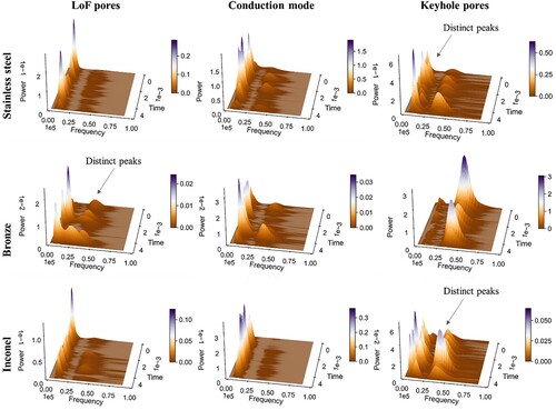
Though the frequency domain analysis gives the frequency components in a signal, it lacks the time localisation of frequencies. The analysis of the AE signals in the frequency domains with time localisation via Wavelet transformation (WT) (Mallat 2009) is presented in this section. The Continuous Wavelet Transformation (CWT) was carried on the filtered AE signals on window sizes of 5 ms. The CWT was calculated on the acoustic signals with the mother wavelet as Morlet (Lin and Qu 2000), as it has a very good approximation error compared to other mother wavelets (Cohen 2019). The wavelet transforms are represented in a 3-dimensional (3D) plot in Figure 9. In this figure, in order to have the distinct peaks visible, the scale of each figure had to be adapted. As for the frequency domain, the wavelet coefficient values were also found to be in the range of around 0–60 kHz for all regimes and alloys. This figure has been depicted with absolute values to show how the intensity of temporal frequency components corresponding to acoustic signals originates during the laser's interaction on different alloys in the process zone. These results also corroborate with the study results made in the frequency domain analysis in Section 3.2. Figure 9 indicates that the values were not continuous with the time scale, and plots appeared in the form of distinct peaks as indicated in the figure by arrows. Also, the wavelet coefficient values were dominant at around 10 kHz for LoF pores in Inconel and stainless steel. In contrast, the wavelet coefficient values for bronze were greater at around 40 kHz for keyhole pores, still to be correlated with a higher energy density. For Inconel, similar to the results of frequency domain analysis of the regime conduction mode, the wavelet coefficient values were observed to be around 10 kHz, whereas they were much higher than the other two regimes. As the resonant sensor was used in this study, the peaks across different regimes for the three materials were populated around 20 and 40 kHz. But it should be noted that irrespective of similarity in the population of the peaks, they carry different intensity values, which is a statistical indicator that laser-material interaction across material and within regimes are different. Based on the distribution and intensity of the wavelet energy coefficients, it can be concluded that the time-resolved frequency features computed using WT will allow the classification of regimes and alloys during real-time monitoring.

Figure 9. 3D wavelet representation of the AE signal for three laser regimes occurring in stainless steel, bronze and Inconel depicting the absolute intensities in temporal frequency distribution among the alloys.

It is important to state that the statistical study in Section 3 primarily focuses on understanding and correlating acoustic emissions when laser interacts with a material causing different regimes. Hence, we have not tried to monitor or localise defects that form due to different process regimes inside the process zone.

4. t-SNE visualisation

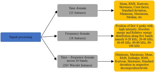
The visualisation of the plots corresponding to the three regimes in Section 3 motivates extracting statistical features from each one to be used as inputs for ML models. A total of 304 features, as listed in Figure 10, were calculated based on a few works focused on classification in material processing (Pandiyan et al. 2020; Pandiyan et al. 2018) using standard python libraries such as NumPy, Scipy, etc. (Lee et al. 2019; Harris et al. 2020) with 23 features from the time domain, 18 features from the frequency domain, and 263 features from the time–frequency domain.

Figure 10. A comprehensive list of statistical features extracted for training the ML model in this work.

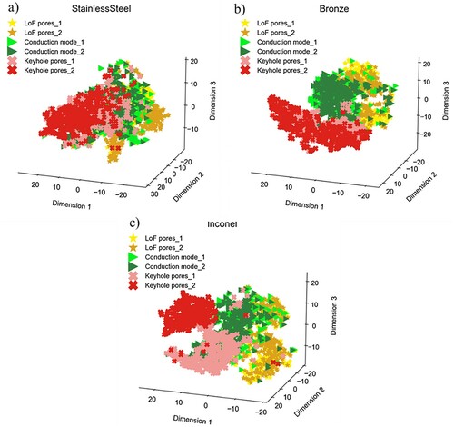
Prior to feeding them into the ML models for classification, finding correlations between them will help choose ML model complexity. With the numerous statistical features calculated from the three domains, the search for recognisable correlations becomes problematic. Dimensional reduction techniques such as t-SNE enable the visualisation of high-dimensional datasets by their projection into the lower-dimensional space, from which they can be easily recognised. t-SNE is a dimensionality reduction technique that non-linearly models the neighbour's probability distribution around each point for mapping the input multi-dimensional data into a lower-dimensional space. In this context, compared to other non-linear dimensionality techniques, t-SNE can retain both the local and global structure of the data simultaneously, enabling data exploration and cluster visualisation in a low-dimensional space (Maaten and Hinton 2008). Since it is a dimensionality reduction technique, the input features after computation is no longer identifiable. In our case, the acoustic features (304 features for a window of 5 ms) from the time, frequency, and time–frequency domains, that were previously discussed were the inputs to perform the t-SNE computation. The motivation to use t-SNE is to interpret and visualise a lower dimension representation to ensure that selected statistical features can form distinct clusters in the lower dimension space.

The perplexity is a hyper-parameter, which gives a ratio of preserving the data's local structure (number of neighbours) and global structure (overall shape). For the perplexity parameter, a value of 10 was chosen after an exhaustive search to visualise the low feature space representation on the AE data acquired during the experiments, and the results are presented in Figure 11. In this figure, the features for each regime are plotted in two shades of colour depending on whether the set of parameters 1 or 2 in Table 2 for a given regime was used. A movie rotating the results can be seen in the supplementary material (https://www.empa.ch/web/s204/lpbf_materials_ae_ml). In Figure 11, the t-SNE plots show that the three regimes (LoF pores, conduction mode, and keyhole pores) appear as distinctive clusters independently of the alloy. There is no drastic change when changing the number of process parameters from 1 to 2 to define a regime. The primary objective of t-SNE was to check the presence of clusters and also to visualise them. Nevertheless, a slight overlap among the three regimes exists for stainless steel (see Figure 11 (a)).

Figure 11. Low-dimension feature space representation using t-SNE with perplexity  = 10 for three different regimes in the LPBF processing of stainless steel, bronze, and Inconel. Subscripts 1 and 2 indicate the number of process parameters considered to define a regime.

5. Classification results for different process regimes and materials

In 2018, Shevchik et al. (Shevchik et al. 2018) demonstrated that they could classify AE signals for the categories LoF pores, conduction mode, and keyhole pores with an accuracy ranging from 83 to 89% for 316L. To achieve these results, they acquired the AE data with a highly sensitive optoacoustic sensor (Fibre Bragg Grating (FBG)). The acoustic features were the relative energies of the WT's narrow frequency bands extracted from all signals. The window size was 160 ms. This section aims to generalise the findings for other metals but using a simple, low-cost microphone, multi-process parameters, and with a window size reduced by a factor of 32 (5 ms). Having two process parameters per category is important to extend the process phase space. The latter is of high importance as it allows a more precise location when the process changes from a ‘defect-free regime to a defect regime (e.g. from conduction mode to keyhole pores).

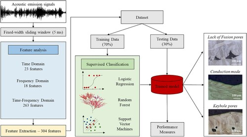
In this section, the extracted time, frequency, and time–frequency domain features from windows of 5 ms are concatenated to form a vector made out of 304 features. These features will be the input of the selected ML algorithms for classifying the three categories. For each of the three categories – LoF pores, conduction mode, and keyhole pores from the LPBF process – a discrete label was assigned for each alloy. The schematic flow of the monitoring methodology is illustrated in Figure 12. A dataset consisted of 3000 rows of features (3000 X 304) and their corresponding ground truth classifier labels for each alloy. The dataset prepared for all three alloys was balanced, with 1000 rows corresponding to each category. The dataset was stochastically split into two subsets, with 70% for training and 30% for testing. This approach simulated real-life conditions where the trained system has to operate with new input data (the test subset). The ML classification models were trained in a supervised manner on the training dataset with the help of the Scikit-learn ML library (Pedregosa et al. 2011). The robustness of the trained model was evaluated by comparing the model's predictions on the test set with the ground truth.

Figure 12. Schematic flow of the monitoring methodology in the LPBF process for the three ML models. The acoustic signals are divided into fixed-width sliding windows of 5 ms, then 304 features are extracted and feeded to the 3 ML algorithms. 70% of the data are used for training, and 30% are kept for testing. The objective is to classify the different regimes (LoF pores, conduction mode, keyhole pores).

Three ML algorithms based on different complexities are used to perform the three alloys’ classification task for comparison. The three ML algorithms selected for the classification tasks are Logistic Regression (LR), Random Forest (RF), and Support Vector Machines (SVM). The logistic regression model combines linear regression and the sigmoid function to return probability values, which can then be mapped to the three discrete categories. The Random forest algorithm used in this work for the classification task had 100 decision trees, and the splits were based on entropy (Pedregosa et al. 2011). Finally, the SVM algorithm used radial basis function (RBF) kernel during training for performing classification.

As an alternative to the use of the extracted features for the classification task, a CNN fed by the raw acoustic signals for the individual alloys is also used in this study. The CNN was preferred over other neural network architectures such as recurrent networks to better compare with ML algorithms, using a vector input. The CNN architecture used to classify the mechanisms for all the individual alloys is illustrated in Figure 13. This architecture design was inspired based on the VGG-16 model (Simonyan and Zisserman 2014) and included five layers with a kernel size of 16. The total number of kernels for the first layer was four and was doubled across each layer, eventually leading to a total number of kernels to 64 in the fifth convolutional layer. A stride of 1 and a padding of 0 was applied across all five convolutional layers. Each layer, except the final fully connected layer, after 1D convolution, was batch normalised before applying the Rectified Linear Units (ReLU) activation function.

Figure 13. An illustration of the CNN architecture used in this work with five convolutional layers and fully connected layers.

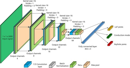
As stated, the CNN network's input was the raw acoustic signal with windows of 5 ms, which is a time-series signal consisting of 5,000 data points. During the network training for the individual alloys, the weight was updated by back-propagating the cross-entropy loss. The model's training for 300 epochs, with a batch size of 100 and a learning rate of 0.01 lasted for two hours. Out of the 3,000 rows of raw signals (1,000 rows for each category), 70% of the rows were stochastically picked for training with equal weight to the categories, and the remaining 30% was used for testing the model performance. The training of the network was done using the PyTorch library and a Titan RTX Nvidia GPU. To avoid overfitting, batch normalisation was applied across layers in the CNN model. Additionally, it was also ensured that the datasets were shuffled across epochs.

5.1. Origin of the acoustic emission features

In this work, a microphone PAC AM4I (Physical Instrument, Germany) was used, which is a high sensitivity airborne sensor. Obviously, such a non-contact sensor captures any acoustic signals (or sounds) reaching it. Their origins are multiple, and the main ones can be summarised as workplace environment, machine and laser noises, and laser-material interactions. The latter is directly related to the process regimes and so the selected categories (LoF pores, conduction mode, keyhole pores). Under such circumstances and for this study, it is imperative to demonstrate that the features used for the classification task come solely from the categories; this is the core objective of this sub-section.

To address this issue, experiments with the same process parameters for all three alloys for the categories LoF pores and keyhole pores (bold red values) in Table 2 were performed. It was not possible for the category conduction mode due to the distinct properties of the selected alloys (stainless steel, bronze and Inconel). When the same process parameter leads to a single process regime for all three alloys, only the laser-material interaction is not identical, caused by the differences in the optical, mechanical, and thermal properties. Consequently, if the features extracted from the microphone are related to this laser-material interaction, it will be possible to classify with high accuracy the alloys using the categories LoF pores and keyhole pores (bold red values) separately in Table 2. In contrast, the classification results being poor would have implied that the features originated from either the workplace environment, machine or laser noises, or process parameters.

The 3 by 3 confusion matrix for the classification of three alloys for the categories LoF pores and keyhole pores using the four algorithms (LR, SVM, RF and CNN) are shown in Table 3, giving the categories (stainless steel, bronze, Inconel) (in rows) versus the ground truth (in columns). The accuracy for the classification in Table 3 is defined based on the number of true positives divided by the total number of tests in each category. These values are given in the diagonal cells of Table 3 (dark grey cells). The misclassifications or the classification errors are computed as the sum of the false positives and false negatives divided by the total number of the tests for each category. These corresponding values are filled in off-diagonal row cells. For example, the classification accuracy of the category stainless steel using the RF model for LoF pores, in violet in Table 3, is 98%. The classification error is 1% with the categories bronze and Inconel. From this table, it is observed that most classification results are higher than 95% independently of the category, alloy and algorithm used. With these results, the obvious conclusion is that the features extracted from the microphone indeed represent the laser-material interaction and the associated process regime.

Table 3. Confusion matrices of the LR, SVM, RF and CNN models trained on the laser regimes across three alloys. Tables for the classification accuracy results in the three alloys. The classification results in each cell are organised as follows: LR (Bold), SVM (Normal), RF (Italics), and CNN (Bold Italics). All values are in %.

	LoF pores			Keyhole pores
Ground truth Classification accuracy [%]	Stainless steel	Bronze	Inconel	Stainless steel	Bronze	Inconel
Stainless steel	99	1	0	95	0	5
	98	1	1	96	0	4
	100	0	0	97	0	3
	100	0	0	97	3	0
Bronze	0	98	2	0	100	0
	0	96	4	0	100	0
	1	99	0	0	100	0
	1.5	97	1.5	5	95	0
Inconel	1	0	99	5	1	94
	1.5	1.5	97	9	1	90
	1	1	98	11	1	88
	0	1	99	1	0	99

5.2. One on one alloy classification

The previous sub- section demonstrated that the AE features are related to the laser-material interaction and associated process regimes (categories LoF pores, conduction mode, and keyhole pores). As already mentioned, in 2018, Shevchik et al. (Shevchik et al. 2018) classified the AE signals for one of the selected alloy (stainless steel – 316L) and for the same categories using an FBG as an airborne opto-acoustic sensor. However, they used only one process parameter per category, which restrains the process phase space. It was decided here to add a second process parameter for each category to increase the process phase space and to demonstrate that our approach is valid for multi-process parameters.

The 3 by 3 confusion matrix for the classification of three mechanisms and three alloys using the three ML models using the extracted features (LR, SVM, and RF) are shown in Table 4. As for Section 5.1, although the ML algorithms vary in terms of complexity and implementation, they all had excellent accuracy. Performance measure experiment with 30% test dataset and 304 features on the LR model had an average classification accuracy of 90.3% for stainless steel, 98.6% for bronze, 98% for Inconel. From the confusion matrices, we can interpret that only a minimum fraction of samples is misclassified. Consequently, three main conclusions can be drawn. First, the classification accuracy is not sensitive to the ML algorithms. Second, the classification accuracy results demonstrate that not only the conduction mode mechanism can be distinguished from defective regimes, but it is possible to differentiate the pore formation regime (LoF pores and keyhole pores). Finally, considering the wide range of metals used, the proposed approach is robust for an extensive range of materials for classification on the explicit condition that the acoustic features corresponding to the materials of interest are part of the training database.

Table 4. Confusion matrix (results of the classification accuracy) of the LR, SVM, RF, and CNN models trained on each individual alloy dataset. The classification results in each cell are organised as follows: LR (Bold), SVM (Normal), RF (Italics), and CNN (Bold Italics), All values are in %.

	Stainless steel			Bronze Inconel			Inconel
Ground truth Classification accuracy [%]	LoF pores	Conduction mode	Keyhole pores	LoF pores	Conduction mode	Keyhole pores	LoF pores	Conduction mode	Keyhole pores
LoF pores	92	0	8	100	0	0	99	0	1
	87	0	13	100	0	0	99	2	1
	93	1	6	98	0	2	98	0	2
	93	7	0	98	2	0	99	1	0
Conduction mode	0	91	9	0	99	1	2	98	0
	0	93	7	0	100	0	0.5	99	0.5
	0	97	3	0	99	1	2	98	0
	5.5	89	5.5	3.5	96.5	0	0	99	1
Keyhole pores	5	7	88	1	2	97	1	2	97
	3.5	9.5	87	1	3	96	2	3	95
	6	6	88	0	1	99	3	4	93
	0	3.5	96.5	0	3	100	1.5	2.5	96

Table 4 also shows the 3 by 3 confusion matrices using the proposed CNN architecture. Although the base CNN architecture used for the classification task was the same as in Section 5.1, their performance was different. The average CNN prediction accuracy in bronze was higher at 98.2%, followed by Inconel (98%) and stainless steel (92.8%). The CNN network's prediction accuracy suggests that raw signals can also be used directly instead of extracting the features independently. Scrutinising Table 4, it is seen that the classification accuracy of stainless steel is lower than in bronze or Inconel. The nature of these results is unknown, but it is due to the non-distinct acoustic patterns inside the signals from the different categories of stainless steel that affect the classification performance.

5.3. One on all alloy classification

The previous section demonstrated that our approach is valid for monitoring while processing single alloy workpieces. Still, the major drawback of industrial application is twofold. First, a classification model has to be built for any material used. Second, the correct material-dependent model has to be ‘loaded’ prior to the processing. Any mistakes at this stage will result in the loss of raw material, machining time, and human resources. Thus, instead of developing one individual classification model for each material, a single classification model was also trained to classify the regimes irrespective of the material by grouping the three alloy datasets according to the ground-truth labels. This approach will answer question (ii) in the introduction.

Similarly to Table 4, Table 5 shows the 3 by 3 confusion matrices for the three regimes on the combined dataset for all ML algorithms. The average classification accuracy is slightly lower than the individual models but remains very high, ranging from 90 to 94.6%, depending on the regime and ML algorithm. The CNN model prediction accuracy suggests that raw acoustic signals can also be used for classifying the three process regimes irrespective of the alloy. We can infer that real-time monitoring of multi-materials using a single ML model will be feasible.

Table 5. Confusion matrices of the LR, RF and SVM model trained on the combined alloy dataset and tested for each alloy and process regimes. The classification results in each cell are organised as follows: LR (Bold), SVM (Normal), RF (Italics), and CNN (Bold Italics). All values are in %.

Ground truth  Classification accuracy [%]	LoF pores	Conduction mode	Keyhole pores
LoF pores	97	3	0
	93	1	6
	95	1	4
	90	9.5	0.5
Conduction mode	3	92	5
	0	93	7
	0	97	3
	8	87	5
Keyhole pores	2	5	93
	7	7	86
	3	5	92
	0	4	96

5.4. Cross alloy classification- towards generalisation

In Sections 5.2 and 5.3, we have proven that ML algorithms can classify the categories of the alloys they have been trained for – either in separate or combined models. However, a question remains whether the same models to classify a new, unseen material (See question (i) in the introduction) can be used. To address this question, several classification tasks were performed on alloys that were not part of the training dataset to understand this hypothesis, using three combinations: one on one (e.g. Inconel on stainless steel) and combinations of two alloys on one (e.g. bronze and Inconel on stainless steel). For this study, RF was selected as the significance of the features for classification can be extracted. Out of the 9 possible combinations among the three alloys, 3 cases had poor average classification accuracy (below 50%), 5 had average accuracies around 70%, and 1 had an average accuracy above 80%. To illustrate these results, one case with good classification and another with poor classification are discussed in this section.

As an example of a good classification case, Table 6 (left) shows the 3 by 3 confusion matrix for a classification RF model built from stainless steel and bronze and tested on Inconel for the three different categories. We can interpret that only a minimum fraction of samples between keyhole pores and conduction mode are misclassified. As an example of a poor classification case, the RF model built from stainless steel and Inconel and tested on bronze, also shown in Table 6 (right), was chosen. Scrutinising the different classification results, no trend could be found between alloys’ choice to train the RF model and the alloy on which the model was tested. In other words, it seems not possible to have a universal or generalised model for most metals. Further investigation on identifying the similarity of features distributions between the alloys, with Kullback–Leibler (KL) divergence, will enable us to understand these results. This analysis will be performed in future work.

Table 6. Confusion matrix of the RF model trained on two alloys and tested on a new alloy. Left table is a good case: Bronze and Stainless steel on Inconel, Right table is a bad case: Inconel and Stainless steel on bronze. All values in %.

Stainless steel + Bronze on Inconel Good case (80%)				Stainless steel + Inconel on Bronze Poor case (35%)
Ground truth  Classification accuracy [%]	LoF pores	Conduction mode	Keyhole pores	LoF pores	Conduction mode	Keyhole pores
LoF pores	61	0	39	100	0	0
Conduction mode	0	93	7	0	42	58
Keyhole pores	6	6	88	14	24	62

5.5. Multi-label classification

In Sections 5.2 and 5.3, most of the ML models discussed were able to classify regimes with high confidence on models trained with single material models or different material. In contrast, in Section 5.4, it was shown that features are material dependent and the possibility to have a universal model is low. Considering these facts, it seems possible to classify the regimes and the alloys (See question (iii) in the introduction). Such classification task can be performed via a multi-label classification. If successful, it will bring three significant advantages to the AM community for the LPBF process of different materials. First, using various materials on the same machine to build single material parts, our methodology could be used for automatic process parameters selection. Second, in the case of defect regime detection, it will determine in which of the materials the defect is created. If most defects are localised within one particular material, the machine operator will know that this specific material's process parameters must be enhanced. Finally, the knowledge of the material and regimes could be used as feedback information to adapt the process parameters if regular deviations in quality are detected.

We propose a multi-label classification CNN architecture to classify the regime and the material simultaneously on a given signal window, as illustrated in Figure 14. The architecture used included five layers with a kernel size of 16, followed by three fully connected layers. The flattened fully connected layer is split into two linear layers, out of which one predicts the regime, and the other one predicts the material. The CNN architecture for multi-label classification, as depicted in Figure 14, is an improvised architecture from the CNN architecture used for classifying regimes in mono-materials in Figure 13. The CNN network input was the raw acoustic signal with a window length of 5 ms with two ground truth labels corresponding to the regime and the material. During the network training, weights were updated by back-propagating the summation of the two cross-entropy losses corresponding to the two branches of the output layer. During the network training, weights were updated by back-propagating the summation of the two cross-entropy losses corresponding to the two branches of the linear layer, as shown in Equation (1). 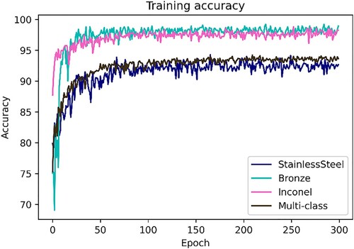(1) $\mathit{L}oss=\mathit{C}rossentropyLoss{1}_{\mathit{m}echanism}+\mathit{C}rossentropyLoss{2}_{\mathit{m}aterial}$(1) The network was trained for 300 epochs, with a batch size of 100 and a learning rate of 0.01 lasted for two hours. Figure 15 confirms the network's accuracy in classifying regimes and alloys increases with training and update of the weights.

Figure 14. A illustration of the multi-label CNN architecture used in this work with five convolutional layers and two branches of fully connected layers.

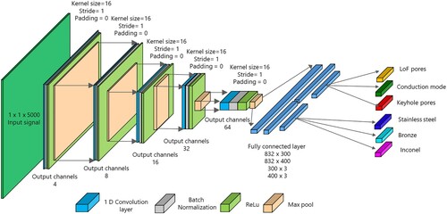
Figure 15. Accuracy curves confirming that CNN models trained for classifying regimes on individual materials and multi-materials learn with training epochs.

The newly configured CNN network for multi-label had the AE raw signals as inputs data. The multi-label classification of the mechanism and the alloy was performed simultaneously, and their accuracy is shown in Table 7. From this table, the overall classification accuracies were 93.3% for the process regimes and 94% for the alloys. Considering the selected process parameters for the process regimes and alloys (See Table 2), these results are of utmost importance for two reasons. First, it establishes that our approach can be successfully applied as a robust and low-cost in situ and real-time process monitoring of multi-material LPBF processes. Second, it confirms the results of Section 5.1; the features used for the classification task originated from the laser-material interaction and the associated process regime. Had it been the process parameters, the classification accuracies for the materials in Table 7 would not exceed 77.6%. As a reminder, for the process regimes, LoF pores and keyhole pores, one set of process parameters was identical for all alloys (bold red values in Table 1), and so it would have equal probability to be classified for any of the three alloys. In other words, these two common process parameters would classify the material correctly with a maximum probability of 33.3%. In contrast, it would be 100% for the other four process parameters, giving the 77.6% (466 out of 600).

Table 7. Confusion matrices of the multi-label CNN model trained on two ground-truth labels. Left table: classification accuracy on the regimes. Right table: classification accuracy on the materials. All values are in %.

	Process regimes (93.3%)				Materials (94.0%)
Ground truth Classification accuracy [%]	LoF pores	Conduction mode	Keyhole pores	Ground truth Classification accuracy [%]	Stainless steel	Bronze	Inconel
LoF pores	93.0	6.5	0.5	Stainless steel	97.0	2.0	1.0
Conduction mode	6.0	91.0	3.0	Bronze	2.0	91.0	7.0
Keyhole pores	0.5	3.5	96.0	Inconel	0.5	5.5	94.0

5.6. Summary of the classification tasks

The results of the classification tasks in this section can be summarised as follows.

• We demonstrated that the AE signatures used for the classification task are strongly related to the laser-material interaction and are unique for each material.

• When coupled with ML algorithms, the features from low-cost airborne acoustic sensors can classify the type of defect regimes (regimes) with very high confidence irrespective of the materials considered.

• The classification of defect regimes irrespective of the material based on a single ML model is feasible by combining the dataset from different alloys.

• The generalisation of the classification of LPBF defects to other (untrained) alloys cannot be made, as the acoustic signals representing the defect formation mechanisms are material-dependent. Failure of generalisations have the positive outcome of successful classification of alloys and regimes simultaneously.

• The multi-label CNN model proposed in this work can simultaneously identify the processing regime and the alloy, with excellent accuracy.

6. Conclusions

This contribution presents an analysis of the AE signals acquired during LPBF processing of three metallic alloys: stainless steel (316L), bronze (CuSn₈), and Inconel (Inconel 718). The experiments were conducted in a custom-designed LPBF machine equipped with an acoustic sensor. The AE sensor used is the PAC AM4I sensor, an airborne sensor with a frequency response in the range of 1–100 kHz. Data acquisitions are made with an Advantech DAQ system at a sampling rate of 1 MHz to record the AE during the experiments. Different laser powers and laser velocities were used to produce overlapping line tracks to simulate three major material qualities (regimes) in LPBF: LoF pores, conduction mode, and keyhole pores. This main contribution objective focuses on the correlation of the three regimes with their corresponding AE signals. The acoustic data resolved in three different domains (time, frequency, and time–frequency) were statistically quantified and visualised to characterise the three regimes for all three alloys. The following generalised conclusions based on the experimental results are summarised below.

Airborne AE is a potential contender for real-time monitoring when processing different materials. They can capture discrete AE signatures corresponding to different laser-material interaction regimes across different alloys. The statistical distribution of different time-domain features among the regimes for all three alloys appear to be different, suggesting that they can be used as an input feature to ML algorithms for in situ and real-time monitoring. The frequency distribution of AE signals for the three materials shows that a significant energy concentration is located between 1 and 60 kHz. The frequency peaks were dominant at around 10 and 40 kHz, as the PAC AM4I acoustic sensor's sensitivity is higher in this region. The comparison of the energy concentration in five energy bands divided equally between 1 Hz to 100 kHz showed that these three regimes under study exhibit discrete energy levels for all three alloys. The distinct energy levels corresponding to the different regimes can also be used as a feature input to any ML algorithm for classification. The visualisation of wavelet plots for a time scale of 5 ms suggests that the energy coefficient distributions are almost synonymous with the frequency-domain results. Discrete peaks from the wavelet plot during the line scan experiments assert that the regimes are distinct, and a proper selection of the window size is vital for real-time defect localisation. The feature reduction based on the t-SNE technique hinted that the regimes features are clustered in the feature space irrespective of the three alloys. The visualisation of the clustered feature space suggests that the LPBF process involving Inconel, bronze, and stainless steel is highly dynamic, and only algorithms capable of classifying data in non-linear spaces would be able to identify them.

Traditional ML algorithms such as LR, RF, and SVM were trained on selected features for classification. Apart from these conventional models, CNN was also trained to classify the raw acoustic signals corresponding to the 3 regimes. Very high classification accuracy was obtained from the ML models such as LR (> 90%), RF (> 92%), SVM (> 89%), and CNN (> 92.5%) on the individual alloys. To address the challenge of the LPBF process of different materials, an ML model built from the three materials showed that the acoustic features prove promising for real-time monitoring, as the classification accuracy was higher than 86%. The study also showed that generalisation of the classification of LPBF defects between alloys is not possible in most cases as the acoustic signals representing the regimes are material dependent. Finally, the multi-label CNN results suggest that – apart from classifying the regimes in different materials with good accuracy – it can also be used to classify the alloy and the regime at the same time. This is of great interest for the LPBF process of multiple materials.

In general, these research outcomes confirm that the extraction of acoustic signals and their features in time, frequency, and time–frequency domains – combined with ML – is a promising technique for in situ and real-time quality monitoring for most metals. We also propose data acquisition strategies, data pre-processing, and ML algorithms to build a complete monitoring system for the LPBF process. The study of the phenomena at frequencies higher than 100 kHz requires a contact AE sensor, a work under investigation. Out of the many events in the laser-material interaction zone, only three processing regimes are correlated to acoustic signals in this research work. The feasibility of understanding the acoustic features corresponding to the early detection of other phenomena such as the evolution of microstructure, propagation of cracks, and delamination are also part of our future work. Also, ML models used in this work are discriminative models, which means they draw boundaries in the data space. As the dataspace changes, they are susceptible to error. And as we move from one machine to another, there is a high probability that this data space will change owing to the geometry of the chamber, machine parameters, the initial condition of the powder spread, location of the airborne acoustic sensor etc. Therefore, for the purpose of universality across machines, developments can be foreseen in generative models or techniques like domain adaptation or transfer learning.

Acknowledgment

The authors would like to acknowledge the financial support of the project MoCont from the Strategic Focus Area Advanced Manufacturing (SFA-AM) programme, a strategic initiative of the ETH Board. RDD and RL gratefully acknowledge the generous sponsoring of PX Group to their laboratory.

Disclosure statement

No potential conflict of interest was reported by the author(s).

Additional information

Funding

The authors would like to acknowledge the financial support of the project MoCont from the Strategic Focus Area Advanced Manufacturing (SFA-AM), a strategic initiative of the ETH Board.

Notes on contributors

Rita Drissi-Daoudi

Rita Drissi-Daoudi received her master degree in Mechanical Engineering in solid and structure mechanics with a minor in Material Sciences in 2018 from École Polytechnique Fédérale de Lausanne (EPFL). She is currently working toward her Ph.D. thesis on in-situ acoustic emission monitoring of the laser powder bed fusion process. at École Polytechnique Fédérale de Lausanne (EPFL), at the Thermomechanical Metallurgy Laboratory, Her research includes signal processing and machine learning but is mainly emphasised on defects formation understanding and laser material processing.

Vigneashwara Pandiyan

Vigneashwara Pandiyan is currently a Postdoctoral Researcher at Laboratory for Advanced Materials Processing (LAMP), Empa – Swiss Federal Laboratories for Materials Science and Technology. He completed his Ph.D. from Nanyang Technological University, Singapore under Rolls-Royce @ NTU corp lab. He has 6 + years of experience as a researcher in manufacturing on characterisation, investigation, optimisation, and process development. Prior to joining Empa, he was a research scientist in A*Star – Agency for Science, Technology and Research ARTC, Singapore. He now concentrates on developing, validating, and implementing machine learning models for in-process sensing of manufacturing processes for anomaly detection and process automation based on sensor signatures.

Roland Logé

Roland Logé is a full-time professor currently working at the Materials Institute, École Polytechnique Fédérale de Lausanne (EPFL), Lausanne. Research activities are focused on the control and design of microstructures in metals and alloys through a combination of thermal and mechanical treatments. Phenomena of interest include recrystallisation, grain growth, twinning, texture evolutions, precipitation, phase transformations, variable temperature conditions, and the possibility of concurrent plastic deformation. Different types of metal forming operations are investigated together with the selective laser melting process and its combination with laser shock peening.

Sergey Shevchik

Sergey Shevchik received the master’s degree in control from Moscow Engineering Physics Institute, Moscow, Russia, in 2003, and the Ph.D. degree in biophotonics from General Physics Institute, Moscow, in 2005. He was a Postdoctoral Researcher with General Physics Institute until 2009. Between 2009 and 2012, he was with Kurchatov Institute, Russia, developing image processing for human-machine interfaces. From 2012 to 2014, he was with the University of Bern, Bern, Switzerland, focusing on computer vision systems and multi-view geometry. Since 2014, he has been a Scientist with the Swiss Federal Laboratories for Material Science and Technology, Thun, Switzerland, developing signal processing and machine learning for industrial automatisation. His research interests include signal processing and machine learning for industrial automatisation.

Giulio Masinelli

Giulio Masinelli received the B.Sc. degree in electrical engineering from the University of Bologna, Bologna, Italy, in 2017, and the master's degree in electrical engineering from École Polytechnique Fédérale de Lausanne (EPFL), Lausanne, Switzerland, in 2019. He is currently working toward his Ph.D. thesis with EPFL and the Swiss Federal Laboratories for Material Science and Technology (Empa), Switzerland, mainly developing machine-learning algorithms for data analysis and industrial automation. His research interests include signal processing and machine learning with an emphasis on deep learning applied to embedded systems.

Hossein Ghasemi-Tabasi

Hossein Ghasemi-Tabasi received his PhD in Institute of Materials, École Polytechnique Fédérale de Lausanne (EPFL). His research involves analysis of the Laser powder bed fusion (LPBF) process in different scales to get a better knowledge of laser/matter interaction and melt pool formation for different process parameters and their effect on the metallurgical features (crack formation, microstructure evolution, precipitations) during the manufacturing process. Investigation of crack formation mechanisms in additively manufactured Ni-based superalloys and studying phase transformation in LPBF red-gold samples are two examples of his researches activities during his PhD.

Annapaola Parrilli

Annapaola Parrilli currently a Scientist of the Centre for X-Ray Analytics, Empa – Swiss Federal Laboratories for Materials Science and Technology. She received her PhD in Biomaterials in 2015 from the University of Pisa in Italy. Her primary research goals are directed toward understanding the morphological, densitometric and mechanical characteristics of materials using X-ray analytical tools. Her research activities are focused on X-ray computed micro and nano Tomography, ranging from image acquisition to image processing and quantification.

Kilian Wasmer

Kilian Wasmer received the B.S. degree in mechanical engineering from Applied University, Sion, Switzerland, and Applied University, Paderborn, Germany, in 1999. He received the PhD degree in mechanical engineering from Imperial College London, London, U.K., in 2003. Since 2004, he has been with the Swiss Federal Laboratories for Materials Science and Technology (Empa), Thun, Switzerland, where he started to work on control of crack propagation in semiconductors. He currently leads the group of dynamical processes in the Laboratory for Advanced Materials Processing at Empa, Thun, Switzerland. Previously, he had focused his work on process development, process monitoring, and quality control via in situ and real-time observation of complex processes using acoustic and optical sensors in various fields such as in tribology, fracture mechanics, and laser processing. His research interests include materials deformation and wear, crack propagation prediction and material-tool interaction in particular laser material processing (e.g. welding, cutting, drilling, marking, cladding, additive manufacturing, etc.). Dr Wasmer is in the Director committee for additive manufacturing of Swiss Engineering. He is also a member of Swiss tribology, European Working Group of Acoustic Emission, Swissphotonics, and Deutsche Gesellschaft für Zerstörungsfreie Prüfung.

References

- Aboulkhair, Nesma T, Nicola M Everitt, Ian Ashcroft, and Chris Tuck. 2014. “Reducing Porosity in AlSi10Mg Parts Processed by Selective Laser Melting.” Additive Manufacturing 1: 77–86.
- Bartlett, Maurice Stevenson. 1948. “Smoothing Periodograms from Time-Series with Continuous Spectra.” Nature 161 (4096): 686–687.
- Caggiano, Alessandra, Jianjing Zhang, Vittorio Alfieri, Fabrizia Caiazzo, Robert Gao, and Roberto Teti. 2019. “Machine Learning-Based Image Processing for on-Line Defect Recognition in Additive Manufacturing.” CIRP Annals 68 (1): 451–454.
- Chen, Changming, Radovan Kovacevic, and Dragana Jandgric. 2003. “Wavelet Transform Analysis of Acoustic Emission in Monitoring Friction Stir Welding of 6061 Aluminum.” International Journal of Machine Tools and Manufacture 43 (13): 1383–1390.
- Chua, Zhong Yang, Il Hyuk Ahn, and Seung Ki Moon. 2017. “Process Monitoring and Inspection Systems in Metal Additive Manufacturing: Status and Applications.” International Journal of Precision Engineering and Manufacturing-Green Technology 4 (2): 235–245.
- Coeck, Sam, Manisha Bisht, Jan Plas, and Frederik Verbist. 2019. “Prediction of Lack of Fusion Porosity in Selective Laser Melting Based on Melt Pool Monitoring Data.” Additive Manufacturing 25: 347–356.
- Cohen, Michael X. 2019. “A better way to define and describe Morlet wavelets for time-frequency analysis,” NeuroImage 199: 81–86. doi: https://doi.org/10.1016/j.neuroimage.2019.05.048
- Cunningham, Ross, Cang Zhao, Niranjan Parab, Christopher Kantzos, Joseph Pauza, Kamel Fezzaa, Tao Sun, and Anthony D Rollett. 2019. “Keyhole Threshold and Morphology in Laser Melting Revealed by Ultrahigh-Speed x-ray Imaging.” Science 363 (6429): 849–852.
- DebRoy, Tarasankar, H. L. Wei, J. S. Zuback, T. Mukherjee, J. W. Elmer, J. O. Milewski, Allison Michelle Beese, A. de Wilson-Heid, A. De, and W. Zhang. 2018. “Additive Manufacturing of Metallic Components–Process, Structure and Properties.” Progress in Materials Science 92: 112–224.
- Dowling, L., J. Kennedy, S. O'Shaughnessy, and D. Trimble. 2020. “A Review of Critical Repeatability and Reproducibility Issues in Powder bed Fusion.” Materials & Design 186: 108346.
- du Plessis, Anton, Ina Yadroitsava, and Igor Yadroitsev. 2020. “Effects of Defects on Mechanical Properties in Metal Additive Manufacturing: A Review Focusing on X-ray Tomography Insights.” Materials & Design 187: 108385.
- Everton, Sarah K, Matthias Hirsch, Petros Stravroulakis, Richard K Leach, and Adam T Clare. 2016. “Review of in-Situ Process Monitoring and in-Situ Metrology for Metal Additive Manufacturing.” Materials & Design 95: 431–445.
- Forien, Jean-Baptiste, Nicholas P Calta, Philip J DePond, Gabe M Guss, Tien T Roehling, and Manyalibo J Matthews. 2020. “Detecting Keyhole Pore Defects and Monitoring Process Signatures During Laser Powder bed Fusion: A Correlation Between in Situ Pyrometry and ex Situ X-ray Radiography.” Additive Manufacturing 35: 101336. doi: https://doi.org/10.1016/j.addma.2020.101336.
- Ghasemi-Tabasi, Hossein, Jamasp Jhabvala, Eric Boillat, Toni Ivas, Rita Drissi-Daoudi, and Roland E Logé. 2020. “An Effective Rule for Translating Optimal Selective Laser Melting Processing Parameters from one Material to Another.” Additive Manufacturing 36: 101496.
- Goh, Guo Dong, Swee Leong Sing, and Wai Yee Yeong. 2021. “A Review on Machine Learning in 3D Printing: Applications, Potential, and Challenges.” Artificial Intelligence Review 54: 63–94. doi:https://doi.org/10.1007/s10462-020-09876-9
- Gong, Haijun, Khalid Rafi, Hengfeng Gu, Thomas Starr, and Brent Stucker. 2014. “Analysis of Defect Generation in Ti–6Al–4 V Parts Made Using Powder bed Fusion Additive Manufacturing Processes.” Additive Manufacturing 1: 87–98.
- Grasso, Marcoluigi, Aligokhan G. Demir, Barbara Previtali, and Biancamaria M. Colosimo. 2018. “In Situ Monitoring of Selective Laser Melting of Zinc Powder via Infrared Imaging of the Process Plume.” Robotics and Computer-Integrated Manufacturing 49: 229–239.
- Gu, Hongping, and Walt W Duley. 1996. “Resonant Acoustic Emission During Laser Welding of Metals.” Journal of Physics D: Applied Physics 29 (3): 550.
- Gu, Dongdong D., Yifu F. Shen, J. L. Yang, and Y. Wang. 2006. “Effects of Processing Parameters on Direct Laser Sintering of Multicomponent Cu Based Metal Powder.” Materials Science and Technology 22 (12): 1449–1455.
- Harris, Charles R, K. Jarrod Millman, Stéfan J van der Walt, Ralf Gommers, Pauli Virtanen, David Cournapeau, Eric Wieser, Julian Taylor, Sebastian Berg, and Nathaniel J Smith. 2020. “Array Programming with NumPy.” Nature 585 (7825): 357–362.
- Heeling, Thorsten, Michael Cloots, and Konrad Wegener. 2017. “Melt Pool Simulation for the Evaluation of Process Parameters in Selective Laser Melting.” Additive Manufacturing 14: 116–125.
- Hooper, Paul A. 2018. “Melt Pool Temperature and Cooling Rates in Laser Powder bed Fusion.” Additive Manufacturing 22: 548–559.
- Jerri, Abdul Jabbar. 1977. “The Shannon Sampling Theorem—Its Various Extensions and Applications: A Tutorial Review.” Proceedings of the IEEE 65 (11): 1565–1596. doi:https://doi.org/10.1109/PROC.1977.10771.
- Jiang, Jingchao, Chunling Yu, Xun Xu, Yongsheng Ma, and Jikai Liu. 2020. “Achieving Better Connections Between Deposited Lines in Additive Manufacturing via Machine Learning.” Math. Biosci. Eng 17 (4). https://doi.org/https://doi.org/10.3934/mbe.2020191
- Khairallah, Saad A, Andrew T Anderson, Alexander Rubenchik, and Wayne E King. 2016. “Laser Powder-bed Fusion Additive Manufacturing: Physics of Complex Melt Flow and Formation Mechanisms of Pores, Spatter, and Denudation Zones.” Acta Materialia 108: 36–45.
- Khanzadeh, Mojtaba, Sudipta Chowdhury, Mohammad Marufuzzaman, Mark A Tschopp, and Linkan Bian. 2018a. “Porosity Prediction: Supervised-Learning of Thermal History for Direct Laser Deposition.” Journal of Manufacturing Systems 47: 69–82.
- Khanzadeh, Mojtaba, Wenmeng Tian, Aref Yadollahi, Haley R Doude, Mark A Tschopp, and Linkan Bian. 2018b. “Dual Process Monitoring of Metal-Based Additive Manufacturing Using Tensor Decomposition of Thermal Image Streams.” Additive Manufacturing 23: 443–456.
- King, Wayne E, Andrew T Anderson, Robert M Ferencz, Neil E Hodge, Chandrika Kamath, Saad A Khairallah, and Alexander M Rubenchik. 2015. “Laser Powder bed Fusion Additive Manufacturing of Metals; Physics, Computational, and Materials Challenges.” Applied Physics Reviews 2 (4): 041304.
- King, Wayne E, Holly D Barth, Victor M Castillo, Gilbert F Gallegos, John W Gibbs, Douglas E Hahn, Chandrika Kamath, and Alexander M Rubenchik. 2014. “Observation of Keyhole-Mode Laser Melting in Laser Powder-bed Fusion Additive Manufacturing.” Journal of Materials Processing Technology 214 (12): 2915–2925.
- Kurzynowski, Tomasz, Edward Chlebus, Bogumiła Kuźnicka, and Jacek Reiner. 2012. “Parameters in Selective Laser Melting for Processing Metallic Powders.” Paper presented at the high power laser materials processing: lasers, beam delivery, diagnostics, and applications.
- Le-Quang, T., S. A. Shevchik, B. Meylan, F. Vakili-Farahani, M. P. Olbinado, A. Rack, and K. Wasmer. 2018. “Why is in Situ Quality Control of Laser Keyhole Welding a Real Challenge?” Procedia CIRP 74: 649–653. doi: https://doi.org/10.1016/j.procir.2018.08.055.
- Lee, Gregory R, Ralf Gommers, Filip Waselewski, Kai Wohlfahrt, and Aaron O’Leary. 2019. “PyWavelets: A Python Package for Wavelet Analysis.” Journal of Open Source Software 4 (36): 1237.
- Lin, Jing, and Liangsheng Qu. 2000. “Feature Extraction Based on Morlet Wavelet and its Application for Mechanical Fault Diagnosis.” Journal of Sound and Vibration 234 (1): 135–148.
- Maaten, Laurens van der, and Geoffrey Hinton. 2008. “Visualizing Data Using t-SNE.” Journal of Machine Learning Research 9 (Nov): 2579–2605.
- Mallat, Stéphane. 2009. A Wavelet Tour of Signal Processing. 3rd ed. Boston: Academic Press.
- Masinelli, G., S. A. Shevchik, V. Pandiyan, T. Quang-Le, and K. Wasmer. 2021. “Artificial Intelligence for Monitoring and Control of Metal Additive Manufacturing.” In Industrializing additive manufacturing. Proceedings of AMPA2020, edited by M. Meboldt, and C. Klahn, 205–220. doi: https://doi.org/10.1007/978-3-030-54334-1_15
- Mukherjee, T., and Tarasankar DebRoy. 2018. “Mitigation of Lack of Fusion Defects in Powder bed Fusion Additive Manufacturing.” Journal of Manufacturing Processes 36: 442–449.
- Nassar, Abdalla R, Molly A Gundermann, Edward W Reutzel, Paul Guerrier, Michael H Krane, and Matthew J Weldon. 2019. “Formation Processes for Large Ejecta and Interactions with Melt Pool Formation in Powder bed Fusion Additive Manufacturing.” Scientific Reports 9 (1): 1–11.
- Pandiyan, Vigneashwara, Wahyu Caesarendra, Tegoeh Tjahjowidodo, and Hock Hao Tan. 2018. “In-process Tool Condition Monitoring in Compliant Abrasive Belt Grinding Process Using Support Vector Machine and Genetic Algorithm.” Journal of Manufacturing Processes 31: 199–213. doi: https://doi.org/10.1016/j.jmapro.2017.11.014.
- Pandiyan, Vigneashwara, Rita Drissi-Daoudi, Sergey Shevchik, Giulio Masinelli, Roland Logé, and Kilian Wasmer. 2020. “Analysis of Time, Frequency and Time-Frequency Domain Features from Acoustic Emissions During Laser Powder-Bed Fusion Process.” Procedia CIRP 94: 392–397. doi: https://doi.org/10.1016/j.procir.2020.09.1
- Pandiyan, Vigneashwara, Sergey Shevchik, Kilian Wasmer, Sylvie Castagne, and Tegoeh Tjahjowidodo. 2020. “Modelling and Monitoring of Abrasive Finishing Processes Using Artificial Intelligence Techniques: A Review.” Journal of Manufacturing Processes 57: 114–135. doi: https://doi.org/10.1016/j.jmapro.2020.06.013.
- Pandiyan, Vigneashwara, and Tegoeh Tjahjowidodo. 2017. “In-process Endpoint Detection of Weld Seam Removal in Robotic Abrasive Belt Grinding Process.” The International Journal of Advanced Manufacturing Technology 93 (5-8): 1699–1714. doi: https://doi.org/10.1007/s00170-017-0646-x
- Pandiyan, Vigneashwara, and Tegoeh Tjahjowidodo. 2019. “Use of Acoustic Emissions to Detect Change in Contact Mechanisms Caused by Tool Wear in Abrasive Belt Grinding Process.” Wear 436–437: 203047. doi: https://doi.org/10.1016/j.wear.2019.203047
- Pedregosa, Fabian, Gaël Varoquaux, Alexandre Gramfort, Vincent Michel, Bertrand Thirion, Olivier Grisel, Mathieu Blondel, Peter Prettenhofer, Ron Weiss, and Vincent Dubourg. 2011. “Scikit-learn: Machine Learning in Python.” the Journal of Machine Learning Research 12: 2825–2830.
- Qi, Ting, Haihong Zhu, Hu Zhang, Jie Yin, Linda Ke, and Xiaoyan Zeng. 2017. “Selective Laser Melting of Al7050 Powder: Melting Mode Transition and Comparison of the Characteristics Between the Keyhole and Conduction Mode.” Materials & Design 135: 257–266.
- Ren, K., Y. Chew, N. Liu, Y. F. Zhang, J. Y. H. Fuh, and G. J. Bi. 2021. “Integrated Numerical Modelling and Deep Learning for Multi-Layer Cube Deposition Planning in Laser Aided Additive Manufacturing.” Virtual and Physical Prototyping, 16 (3): 318–332. doi: https://doi.org/10.1080/17452759.2021.1922714.
- Scime, Luke, and Jack Beuth. 2018a. “Anomaly Detection and Classification in a Laser Powder bed Additive Manufacturing Process Using a Trained Computer Vision Algorithm.” Additive Manufacturing 19: 114–126.
- Scime, Luke, and Jack Beuth. 2018b. “A Multi-Scale Convolutional Neural Network for Autonomous Anomaly Detection and Classification in a Laser Powder bed Fusion Additive Manufacturing Process.” Additive Manufacturing 24: 273–286.
- Scime, Luke, and Jack Beuth. 2019. “Using Machine Learning to Identify in-Situ Melt Pool Signatures Indicative of Flaw Formation in a Laser Powder bed Fusion Additive Manufacturing Process.” Additive Manufacturing 25: 151–165.
- Scime, Luke, Derek Siddel, Seth Baird, and Vincent Paquit. 2020. “Layer-wise Anomaly Detection and Classification for Powder bed Additive Manufacturing Processes: A Machine-Agnostic Algorithm for Real-Time Pixel-Wise Semantic Segmentation.” Additive Manufacturing 36: 101453.
- Shevchik, S. A, C. Kenel, C. Leinenbach, K. Wasmer. 2018. Acoustic emission for in situ quality monitoring in additive manufacturing using spectral convolutional neural networks, Additive Manufacturing 21: 598–604. doi: https://doi.org/10.1016/j.addma.2017.11.012.
- Shevchik, Sergey A, Tri Le-Quang, Farzad Vakili Farahani, Neige Faivre, Bastian Meylan, Silvio Zanoli, and Kilian Wasmer. 2019. “Laser Welding Quality Monitoring via Graph Support Vector Machine With Data Adaptive Kernel,” In IEEE Access, vol. 7, 93108–93122, doi: https://doi.org/10.1109/ACCESS.2019.2927661.
- Shevchik, S. A, T. Le-Quang, B. Meylan, F. Vakili-Farahani, M. P. Olbinado, A. Rack, G. Masinelli, C. Leinenbach, and K. Wasmer. 2020. “Supervised Deep Learning for Real-Time Quality Monitoring of Laser Welding with X-Ray Radiographic Guidance.” Scientific Report, vol. 10, paper ID: 3389. doi:https://doi.org/10.1038/s41598-020-60294-x
- S. A. Shevchik, G. Masinelli, C. Kenel, C. Leinenbach and K. Wasmer. 2019. “Deep Learning for In Situ and Real-Time Quality Monitoring in Additive Manufacturing Using Acoustic Emission,” in IEEE Transactions on Industrial Informatics, vol. 15, no. 9, pp. 5194–5203. doi: https://doi.org/10.1109/TII.2019.2910524.
- Simonyan, Karen, and Andrew Zisserman. 2014. “Very Deep Convolutional Networks for Large-Scale Image Recognition.” arXiv Preprint ArXiv:1409.1556. https://arxiv.org/abs/1409.1556
- Sing, S. L., C. N. Kuo, C. T. Shih, C. C. Ho, and C. K. Chua. 2021. “Perspectives of Using Machine Learning in Laser Powder bed Fusion for Metal Additive Manufacturing.” Virtual and Physical Prototyping 16 (3): 372–386.
- Spears, Thomas G, and Scott A Gold. 2016. “In-process Sensing in Selective Laser Melting (SLM) Additive Manufacturing.” Integrating Materials and Manufacturing Innovation 5 (1): 16–40.
- Tapia, Gustavo, and Alaa Elwany. 2014. “A Review on Process Monitoring and Control in Metal-Based Additive Manufacturing.” ASME Journal of Manufacturing Science and Engineering 136 (6): 060801. doi: https://doi.org/10.1115/1.4028540
- Thanki, Aditi, Louca Goossens, Raya Mertens, Gabriel Probst, Wim Dewulf, Ann Witvrouw, and Shofeng Yang. 2019. “Study of Keyhole-Porosities in Selective Laser Melting Using X-ray Computed Tomography.” 9th Conference on Industrial Computed Tomography, (iCT 2019), Padova, Italy.
- Van Elsen, Maarten. 2007. Complexity of Selective Laser Melting: a new optimisation approach.”.
- Wasmer, K., C. Kenel, C. Leinenbach, and S. A. Shevchik. 2018. “In Situ and Real-Time Monitoring of Powder-bed AM by Combining Acoustic Emission and Artificial Intelligence.” Presented at Additive Manufacturing for Products and Applications Conference 2017 (AMPA), Zürich, Switzerland, September 13–15, 2017. In Proceedings of Additive Manufacturing in Products and Applications - AMPA2017 - Industrializing Additive Manufacturing, edited by M. Meboldt, and C. Klahn, 200–209. Springer International Publishing: Zürich, Switzerland, doi: https://doi.org/10.1007/978-3-319-66866-6_20.
- Wasmer, Kilian, Tri Le-Quang, Bastian Meylan, and Sergey A. Shevchik. 2019. “In Situ Quality Monitoring in AM Using Acoustic Emission: A Reinforcement Learning Approach.” Journal of Materials Engineering and Performance 28 (2): 666–672. doi: https://doi.org/10.1007/s11665-018-3690-2
- Welch, Peter. 1967. “The use of Fast Fourier Transform for the Estimation of Power Spectra: A Method Based on Time Averaging Over Short, Modified Periodograms.” IEEE Transactions on Audio and Electroacoustics 15 (2): 70–73.
- Wu, Haixi, Yan Wang, and Zhonghua Yu. 2016. “In Situ Monitoring of FDM Machine Condition via Acoustic Emission.” The International Journal of Advanced Manufacturing Technology 84 (5-8): 1483–1495.
- Wu, Haixi, Zhonghua Yu, and Yan Wang. 2017. “Real-time FDM Machine Condition Monitoring and Diagnosis Based on Acoustic Emission and Hidden Semi-Markov Model.” The International Journal of Advanced Manufacturing Technology 90 (5-8): 2027–2036.
- Xiao, Ling, Mingyuan Lu, and Han Huang. 2020. “Detection of Powder bed Defects in Selective Laser Sintering Using Convolutional Neural Network.” The International Journal of Advanced Manufacturing Technology 107: 2485–2496. doi: https://doi.org/10.1007/s00170-020-05205-0
- Yan, Zhaorui, Weiwei Liu, Zijue Tang, Xuyang Liu, Nan Zhang, Mingzheng Li, and Hongchao Zhang. 2018. “Review on Thermal Analysis in Laser-Based Additive Manufacturing.” Optics & Laser Technology 106: 427–441.
- Yap, Chor Yen, Chee Kai Chua, Zhi Li Dong, Zhong Hong Liu, Dan Qing Zhang, Loong Ee Loh, and Swee Leong Sing. 2015. “Review of Selective Laser Melting: Materials and Applications.” Applied Physics Reviews 2 (4): 041101.
- Ye, Dongsen S., Jerry Ying Hsi Fuhy, Y. J. Zhang, G. S. Hong, and Kunpeng P. Zhu. 2018. “Defects Recognition in Selective Laser Melting with Acoustic Signals by SVM Based on Feature Reduction.” MS&E 436 (1): 012020.
- Ye, Dongsen, Geok Soon Hong, Yingjie Zhang, Kunpeng Zhu, and Jerry Ying Hsi Fuh. 2018. “Defect Detection in Selective Laser Melting Technology by Acoustic Signals with Deep Belief Networks.” The International Journal of Advanced Manufacturing Technology 96 (5-8): 2791–2801.
- Yu, Chunling, and Jingchao Jiang. 2020. “A Perspective on Using Machine Learning in 3D Bioprinting.” International Journal of Bioprinting 6 (1): 253. doi: https://doi.org/10.18063/ijb.v6i1.253. eCollection 2020
- Zhang, Bi, Yongtao Li, and Qian Bai. 2017. “Defect Formation Mechanisms in Selective Laser Melting: A Review.” Chinese Journal of Mechanical Engineering 30 (3): 515–527.
- Zhao, Cang, Kamel Fezzaa, Ross W Cunningham, Haidan Wen, Francesco De Carlo, Lianyi Chen, Anthony D Rollett, and Tao Sun. 2017. “Real-time Monitoring of Laser Powder bed Fusion Process Using High-Speed X-ray Imaging and Diffraction.” Scientific Reports 7 (1): 1–11.