In-situ monitoring of the melt pool dynamics in ultrasound-assisted metal 3D printing using machine learning

ABSTRACT

Ultrasound-assisted directed energy deposition (UADED) is a promising technology for improving the properties of printed parts. However, process monitoring during UADED remains a challenge as ultrasound obscures the physical characteristics of DED. Here, the physical phenomena during UADED are captured using in-situ imaging and an unsupervised learning with auto-encoding is proposed to reconstruct images of the melt pool and analyse the features of spatter and plume to achieve the forming quality monitoring. This method enables effectively identifying the dynamic relationship in melt pool-spatter-plume, and the average recognition accuracy for reconstructed images reaches 94.52% during fully connected auto-encoders. Based on recognition results, the spatters during UADED are more intense, but the plume phenomenon is weakened compared to DED. The reason is that the flow mode was changed into reciprocal flow due to ultrasound. Subsequently, experiments indicated the method possessed high accuracy and robustness. The paper aims to provide a reference source for research studies on intelligent monitoring metal 3D printing.

GRAPHICAL ABSTRACT

KEYWORDS:

• Ultrasound-assisted directed energy deposition
• spatters and plume
• image processing
• auto-encoding
• real-time monitoring

Nomenclature
$A_0$	=	the amplitude of UA-DED (μm)
$N_{ϵ}$	=	the ϵ-neighbourhood of x
$c_1,c_2$	=	the first/second centroid of the chosen observation
$c_p$	=	the pth centroid of the chosen observation
$C_p$	=	the set of all observations closest to centroid cp
$\mathit{A}$	=	the weight matrix of the encoder
$\hat{\mathit{A}}$	=	the weight matrix of the decoder
$k$	=	the number of clustering categories
$S{S}_{\mathrm{B}}$	=	the inter-class variance
$W_k$	=	within-cluster dispersion
$n_q$	=	the total number of data points of class q
$C_q$	=	the set of all data in the class q
$\mathit{U}$	=	the eigenvector matrix
${\sigma }_k$	=	the kth singular value of the matrix Q
$u_k{v}_k$	=	the kth eigenspace
$f\left(x\right)$	=	the encoder’s nonlinear activation function
$K$	=	the clustering centre of PCA
$D$	=	a demonstration dataset
$\mathrm{A}\mathrm{R}\mathrm{I}$	=	the adjusted rand index
$\mathrm{U}\mathrm{A}\mathrm{D}\mathrm{E}\mathrm{D}$	=	ultrasound-assisted directed energy deposition
$f$	=	the frequency of UA-DED (Hz)
$ϵ$	=	the radius of the neighbourhood
$P$	=	Laser power (W)
$f_{\mathrm{r}\mathrm{a}\mathrm{t}\mathrm{e}}$	=	Powder flow rate (r/min)
$v_s$	=	Scan rate (mm/min)
$\mathit{b}$	=	the offset vector of the encoder
$\mathit{c}$	=	the offset vector of the decoder
$N$	=	the number of data
$S{S}_{\mathrm{W}}$	=	the intra-class variance
$B_k$	=	between-cluster dispersion mean
$c_q$	=	the centroid of the class q
$c_E$	=	the centroid of all data
$\mathit{V}$	=	the eigenvector matrix
$\mathit{S}$	=	the diagonal matrix
$\lambda$	=	the eigenvalue of the matrix QTQ or QQT
$g\left(h\right)$	=	the decoder's nonlinear activation function
$E$	=	laser energy density (J/mm2)
$d\left(x,c\right)$	=	the distance metric between x and c
$CH$	=	the Calinski-Harbasz score
$\mathrm{D}\mathrm{E}\mathrm{D}$	=	directed energy deposition

1. Introduction

Improving the forming accuracy and enhancing the mechanical properties are the key to popularising the direct energy deposition (DED) technology. Some advanced means (e.g. magnetic field and ultrasound field) for strengthening mechanical properties were reported in recent years [1–3]. Among them, the promising technology of ultrasound combined with DED was more concern in the study. However, related research on monitoring the forming quality was rarely explored in DED with ultrasound, especially for surface accuracy. Qian et al. found that the surface accuracy of as-built-in DED with ultrasound was poor [4,5], reducing the forming efficiency. Moreover, multi-parameter interaction is an essential factor in the forming accuracy (i.e. scanning speed, powder speed and laser power, ultrasound amplitude). Therefore, to improve the repeatability and reliability, the real-time monitoring of the forming process and controlling the forming accuracy are significant for the wide application in metallic additive manufacturing (AM) with ultrasound.

Recently, the research on the microstructure evolution and mechanical properties of as-built has been hot topics in ultrasound-assisted DED (UADED). The related reports indicated that the cavitation and acoustic streaming caused by ultrasound can change the flow [6–8]. Therefore, During the crystallisation process, the dendrites are affected due to the impact force generated by cavitation and fatigue fracture occurred. It further increases the nucleation rate during the crystallisation and refines the grains [9,10]. Cong and Ning [11] studied the influence of ultrasound frequency on microstructure and mechanical properties in directed energy deposited Inconel 718. The results demonstrated that ultrasound was beneficial to the dissolution of the Laves phase and further changed the mechanical properties of the as-built workpiece. The lowest porosity during DED-fabricated Inconel 718 was achieved at an ultrasonic frequency of 25 kHz, basically due to the elimination of lack-of-fusion and gas entrapped pores [12,13]. Todaro et al. point out that both of as-built samples for the yield strength and the ultimate tensile strength in DED with ultrasound were improved by 12% [4,5]. The application of ultrasound produces predominately equiaxed grains of only a few microns in size with a near-random crystallographic texture. Yang et al. [7] explored the effect of amplitude on the microstructure evolution, tensile properties and microhardness. The results demonstrated that the properties of as-built parts were improved through refining grains. And the degree of grain refinement increases for samples with an increase in amplitude [14,15]. However, the surface quality of as-built parts is very poor in DED with ultrasound and restricts the development of UADED. Therefore, monitoring the deposition process and performing parameter optimisation is an effective means to improve the surface quality of the formed parts and to reduce defects.

The metal-based additive manufacturing condition monitoring is a data-driven method to detect the process state in the production process based on the light, heat, sound, force and other signals [16–19]. Among them, the monitoring of additive manufacturing, based on machine learning, is highly popular. The application of machine learning has been extended to different phases of the AM process (the digital phase, the manufacturing phase and the post-processing phase) [20,21]. More basically, a diversity of machine-learning methods has been developed to analyse the relevant physical phenomena (e.g. melt pool, spatter) to uncover the underlying mechanisms in the printing process [22]. For instance, typical approaches include shallow machine-learning methods, such as conventional neural networks (NN), support vector machine (SVM), Gaussian process (GP) and the latest developments of deep learning methods such as a convolutional neural network (CNN), a deep belief network (DBN) and a long short-term memory (LSTM) network. By characterising and analysing melt pool images with these machine learning methods, complex mapping relationships between the characteristics of the melt pool, spatters and plume and process parameters can be obtained to determine whether the forming quality of as-built parts is abnormal. This method not only reduces the high cost of post-build approaches (e.g. non-destructive inspection by CT-scan, destructive inspection) for inspecting the forming quality of samples but also effectively improves the accuracy. Therefore, it provides a cheaper but more effective alternative to manually annotating data by labelling data based on the proximity of corresponding structural properties. The structural properties of the data are captured by a set of high-quality features from samples. In addition, considering the effect of ultrasound, the dynamic characteristics of the melt pool due to the complex interactions between ultrasound-flow-solidification have changed, which directly affects the prediction of as-built quality in UADED [7]. Detailed quantitative investigation on the characteristics of the melt pool, spatters and plume is necessary during AM.

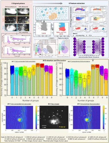
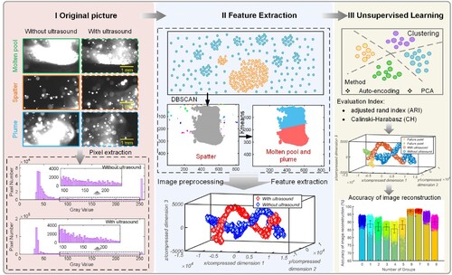
The previous work gives us massive inspiration for monitoring metal 3D printing. In the paper, a machine vision monitoring method combined with high-speed image was adopted, which can detect information of process signatures, e.g. melt pool, spatters and plume. The application of ultrasonic vibration makes the flow, spattering and plume in the melt pool more intense compared with the normal DED process. Therefore, the traditional supervised classification method is not suitable to identify the characteristics of melt pools, spatters and plumes due to its poor robustness. Here, the unsupervised machining was applied to monitor the surface quality of single tracks during DED with ultrasound. The paper structure can be divided into six sections (see Figure 1). Section 2 provides a detailed literature review. In Section 3, we tried to explore the generation mechanisms of the melt pool, spatter and severe plasma plume through the experimental device built during DED and UADED. The original images acquired during the experiment were elaborated in the paper. The new identification method was proposed to analyse the characteristics of the melt pool, spatter and plume in Section 4. Furthermore, the performance of the designed identification method was evaluated in Section 5, and the effects of ultrasound on the cross-section of tracks and the microstructure were discussed during DED and UADED in the paper. Finally, a series of conclusions are shown in Section 6.

Figure 1. The logical framework in the study.

2. Literature review

We survey the papers pertaining to melt pool monitoring and the existing spatters and plume detection techniques. To analyse characteristic information of melt pools, spatters and plumes, the authors attempted to use multiple sensors to obtain first-hand information [16,23–25]. Then, integrating machine learning into AM, the approach can help improve product quality, optimise manufacturing processes and reduce costs. This section is divided into two subsections: (i) Machine learning for melt pool monitoring; (ii) methods for spatters and plume characterisation.

2.1. Machine learning for the melt pool

Machine learning is an artificial intelligence technique that helps to identify patterns in data and generate similar data without human intervention to make decisions or predictions. Overall, the related research in identifying and analysing melt pool image features through machining learning is mainly divided into three categories: supervised, unsupervised and reinforcement learning. Supervised learning enables us to learn from a set of labelled data in the training set so that it can identify un-labelled data from a test set, to characterise the essential characteristics of relevant samples and reveal physical phenomena. Among them, classification and regression are normally two important functions for the prediction of as-built quality in additive manufacturing. Zhang et al. [26] studied the effects of these object characteristics on built quality during LPBF by using SVM and CNN. The experiments showed that the classification accuracy of the CNN was higher than that of the SVM for the as-built. Moreover, based on the CNN architecture, a hybrid CNN approach is further proposed for laser powder bed fusion (LPBF) process monitoring. This method saves image processing steps and can automatically learn spatial and temporal representative features (e.g. melt pool) from raw images [27]. However, supervised learning also has certain disadvantages. That is, only known categories can be effectively predicted in the model.

Unsupervised learning (e.g. clustering, principal component analysis (PCA)) speculates from un-labelled data, which can uncover hidden patterns or group similar data in a given random dataset. It is widely used in anomaly detection. Grasso et al. [16,28] investigated the defects in selective laser melting (SLM) and proposed a method to automatically detect defects by a machine vision system in the visible range, combined with PCA for statistical descriptor selection and K-means clustering for defect detection. Yang et al. [29] presented a novel method called the Layer-wise neighbouring-effect modelling method (L-NBEM) that used a scan strategy to predict melt pool size. Concretely, a fully connected neural network is trained on the data with a new set of features to predict the melt pool area. In a later study, Fathizadan et al. [30] proposed a framework to process melt pool images by a configuration of convolutional auto-encoder neural networks. The result is that the accuracy of feature extraction reached 95%. Subsequently, a control charting scheme based on Hotelling’s T² and S² statistics is developed to monitor the stability of the process. Following the same stream of research, Kim et al. [31] developed a new method based on deep learning to directly estimate the melt pool coordinate position from the melt pool images in AM. In terms of image preprocessing (i.e. image transformation and spatter reduction), a stacked convolutional auto-encoder is used to reduce noises from raw melt-pool monitoring images. Unlike previous work, a new porosity prediction method based on the temperature distribution of the top surface of the melt pool was presented by Khanzadeh et al. [32,33]. To determine the features of melt pool images, they transformed the relevant data into a spherical coordinate system and then utilised biharmonic surface interpolation to smooth and extract feature vectors. Afterwards, these vectors are put into self-organising maps (SOMs) and each image is clustered by SOMs to judge whether it is normal or porous. In addition, to better learn the process-structure–property (PSP) relationships for various AM processes, Ko et al. [34] proposed a novel framework driven by physics-guided machine learning, mainly involving three tiers: (i) knowledge of predictive PSP models and physics, (ii) PSP features of interest and (iii) raw AM data. This framework provided a systematic physics-guided data-driven approach for PSP in AM that combined physics knowledge with the versatility of data-driven machine learning models.

2.2. Spatters and plumes characterisation

The spatters and plume characteristics in metal AM can determine the quality of as-built parts to a certain extent. For obtaining raw data, high-speed camera technology shows great advantages in capturing the spatial dynamic changes and time changes of spatters and plumes in real time [35,36]. At present, related works of literature have reported some detection approaches on spatters and plumes, including traditional computer vision, combined image processing with simple machine learning and complex deep learning models. Typically, Tan et al. explored the characteristics of spatter and extracted the spatters by neural network based on image segmentation in the LPBF [37,38]. The results indicated that the proposed method can extract 80.48% of spatters in only 70 ms. Criales et al. [39] investigated the percentage of spatters in each frame obtained by using a high-speed camera and found that the spatters’ percentage was 20% or more, and in some conditions up to 70%. In addition, Repossini et al. [40] developed a logistic regression model to determine to classify different energy density conditions corresponding to different quality states by analysing the spatter characteristics. A significant increase in the capability to detect under-melting and over-melting conditions is observed by including spatters as process signature drivers. However, only three spatter signatures were investigated because of the limitation of the image-capturing method and the image-processing algorithm. In a later study, Baumgartl et al. [41] proposed a created CNN architecture with depthwise-separable convolutions to train the thermographic data. The results demonstrated the potential of deep learning over classic computer vision techniques for spatter detection. However, the limitation of the proposed method is that it can only detect spatters and delamination. Chebil et al. [42] developed a deep learning architecture (YOLOv4) to the peculiarities of spatter detection. The method established a rapid and automatic control method to evaluate the stability of the LPBF process, using spatters as a process signature.

In summary, considering the coupling effects of laser and ultrasound on melt pool, spatters and plume features, an improved convolutional auto-encoder architecture is constructed by a hybrid data augment and a semi-fixed weight iteration strategy for in-suit monitoring of melt pool in this paper. In the compression structure, the collected raw image data are first subjected to several symmetric transformation data enhancement preprocessing to reduce noise. Then, a semi-fixed weight iteration strategy is provided in the auto-encoding structure, that is, the weights of some layers are fixed, and the weight gradients of the remaining layers decrease. Finally, the feature signals are extracted in the middle layer and clustered in several dense stacks, which respectively belong to several different working conditions. In doing so, compared to typical unsupervised learning, the abilities of anomaly detection and analysing data are further enhanced by improving the iteration method and data compression structure.

3. Experimental section

3.1. Experimental set-up and materials

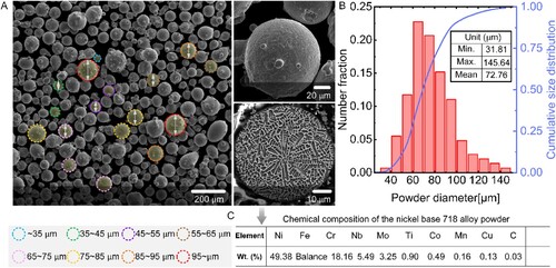
Figure 2 displays a schematic diagram of the experimental set-up for monitoring the laser deposition process and the inner workings of a multilayer auto-encoder neural network for pattern recognition. Considering that the plasma radiation would be overly bright to cover the information of the melt pool, a high-speed camera with a visible waveband cut-off filter was installed on the SVW80C-3D machining centre to collect an angled top view of the melt pool. The cut-off filter can reduce the brightness of the plume with the 400–800 nm visible waveband, which was put in front of the high-speed camera. The SVW80C-3D machining centre includes a laser system with a YLS-2000 fibre laser source (3 mm diameter, as shown in Supplementary Table S1 and Figure S1), a monitor control system, a chamber system, a delivery system for powder, nitrogen and ultrasonic vibration-assisted device. Among them, the maximum power of the laser source is 2000 W with the wavelength range from 1070 nm to 1080 nm coupled to a scanner for laser path control. The ultrasound vibration direction is along the scanning direction, and the calibration results are shown in Figure 2(A). In the process, the view field of 7 × 5 mm² was selected as a sample picture instead of the DED process through lens configuration to guarantee a sufficient spatial resolution. Sufficient information on the melt pool, spatter and the plume was captured in UA DED and DED, along with the 5000 frames sampling rate of a high-speed camera. Moreover, the installation position of the high-speed camera formed an angle of θ = 50° with the horizontal plane. The distance between the front end of the high-speed camera and the cladding surface is 260 mm. In addition, Inconel 718 powder with a size range from 31.81 μm to 145.64 μm was used in DED without and with ultrasound. The morphology, microstructure and composition of the powder are demonstrated in Figure 3. Simultaneously, #45 steel was selected as the substrate during the experiment.

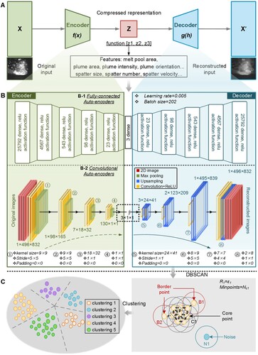
Figure 2. Schematic diagram of a physical-aware framework for monitoring quality in UADED and DED. (A) the in-situ monitoring experiment with a high-speed camera and a high-resolution laser displacement sensor (sampling frequency of 100 kHz) provided by Virtins Technology was used to track and analyse the vibration characteristics of the sample in real-time, including the vibration frequency and amplitude. (B) shows the experimental set-up, including the laser deposition processing centre, ultrasonic vibration device and the high-speed camera system. (C) Illustration of the inner workings of a multilayer auto-encoder neural network.

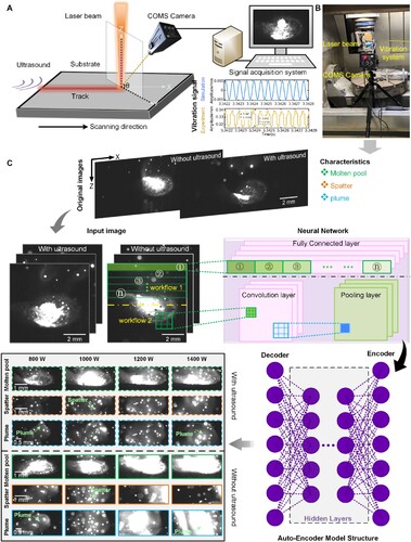
Figure 3. Powder characteristics of Inconel 718. (A) was the morphology and microstructure of powders. (B) was the size distribution of the powders. (C) was the Inconel 718 powder chemical composition.

3.2. Generation mechanisms of the melt pool, spatter and plume signals in UV-A DED

By the analysis of the high-quality images, the information objects (i.e. melt pool, spatter and plume) were selected in the study, as shown in Figure 2C. Here, the basic generation mechanisms of the melt pool, spatter and plume were stated in the paper. During DED, the flowing metal powders melt by absorbing high-density laser energy and quickly transform liquid metal, that is, melt pool. According to Planck's law, the thermal radiation of the melt pool surface can be used for melt pool temperature detection [26,43]. As can be seen, the stable surface of the melt pool was broken due to the introduction of ultrasound in DED. Compared with the non-ultrasound, a depression in the centre of the melt pool was caused, along with fish-scale ripples. The reason is that the inertial force generated by ultrasound is much greater than that of the surface tension [7]. Besides, the tail of the melt pool during DED with ultrasound was extended, and there is an obvious solid–liquid coexistence area at the tail, as shown in Supplementary Figure S2 and Movie S1–S2. For the solidified tracks, a stacking phenomenon was significant. The tracks were much uneven compared with these tracks without ultrasound. For plume generation, the high-density laser beam made plume vapour eject from the inside of the keyhole in DED, which is relatively stable. However, the synergistic effect of ultrasonic vibration and high-density laser beam changed the Marangoni flow and made the upper plume strengthen in UA DED, along with severe chaos. Here, we should try unsupervised learning to identify an analysis of the area of the plume, its size and the direction of the plume during UA DED. In addition, some studies indicated that the spatter was another important indicator to evaluate the as-built quality [44–46]. Surface tensile and recoil pressure caused by evaporation, and the gas entrainment driven by Bernoulli’s effect, were the main reasons for generation spatters during LPBF [47–49]. Unlike that, more severe spatter ejected due to the ultrasound vibration from the melt pool compared with the DED process, along with the chaotic direction. The spatter characteristics of the area of the spatter, direction and the speed rate are very important for the forming quality. Thus, comprehensive information on the melt pool, spatter and plume can help monitor and evaluate the forming quality during the laser deposition process.

3.3. Acquisition of original images

Considering the severe dynamic disturbance in DED with ultrasound, the active vision method with an additional light source was adopted to increase the accuracy of the extracted visual feature (see Figure 2). The 8-bit image captured by a high-speed camera has a greyscale value ranging from 0 to 255, and the original image resolution is 832 × 496 pixels. In addition, the images were randomly selected and the time interval is 0.16 ms. Here, we assume that the velocity of the spatter is constant when the spatters are ejected from the melt pool in a short time. The experiment parameter (laser power, scanning speed, and powder feeding rate) was set as follows, as shown in Table 1. As shown in Figure 2, the motion state of the melt pool and spatters was very severe by introducing ultrasound. During the spatter extraction process, some major factors can interfere with the extraction effect, including the melt pool produced by the laser beam, the residual uncooled melt pools and the plumes, whose luminance was similar to that of the spatters. Therefore, the raw images were preprocessed before feature extraction.

Table 1. Experimental parameters in the study.

Group	Laser power P (W)	Powder flow rate frate (r/min)	Scan rate vs. (mm/min)	Amplitude A0 (μm)
1	600,800,1000,1200,1400	1	360	10
2	1000	1	240,300,360,420,480
3	1000	0.5,1,1.5,2,2.5	360
4	600,800,1000,1200,1400	1	360	none
5	1000	1	240,300,360,420,480
6	1000	0.5,1,1.5,2,2.5	360

4. Image process and feature extraction

4.1. Image preprocessing methodology

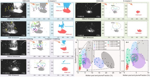
To obtain interesting characteristics from the original images, a hybrid preprocessing method based on DBSCAN (density-based spatial clustering of applications with noise) and K-means++ is presented in the study. Figure 4 shows the complete processing framework for the raw features, including melt pool, spatters and plume. Considering that the grey value of the melt pool image represents the information on melt pool temperature distribution and the flow stability of the melt pool, the grey value was calculated under the different process parameters (see Figure 5). In the study, the grey value was divided into m_b bins and the pixel number in different bins was extracted as melt pool, spatters and plume features. The m_b was 75. When the applied laser power exceeds 800 W, the pixel numbers of greyscale values 252∼255 with ultrasound are significantly lower than those without ultrasound. Combined with the original image analysis, the plume phenomenon is significantly weakened when ultrasonic vibration is applied (see Figure 6). Given the size, distribution and shape feature of spatters in the images, the spatters were divided into multiple dense heaps different from the melt pool and plume based on DBSCAN. For the DBSCAN, it is a density-based clustering algorithm, the main hyperparameters are neighbourhood radius ϵ and min-point N_ϵ, respectively. The method continuously searches for dense clusters which can be connected and then connects them, until no new clusters can be connected. The flow chart of processing the spatters for DBSCAN is shown in Figure 4C. Then, the melt pool and plume are further processed by the K-mean++, as shown in Figure 4D and Supplementary Figure S3.

Figure 4. Overview of the image hybrid preprocessing methodology. (A) The regions of interest extracted from the original image (melt pool, spatters and plumes). (B) Greyscale processing of the original image and grey-level distribution. (C) The preprocessed workflow of spatters by the DBSCAN. (D) The processed logical framework of the melt pool and plume by K-means++.

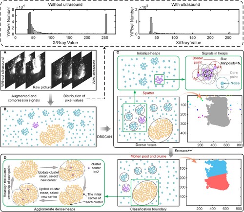
Figure 5. Greyscale distribution of the melt pool, spatter and plume under ultrasound or non-ultrasound conditions. Scale bars 1 mm.

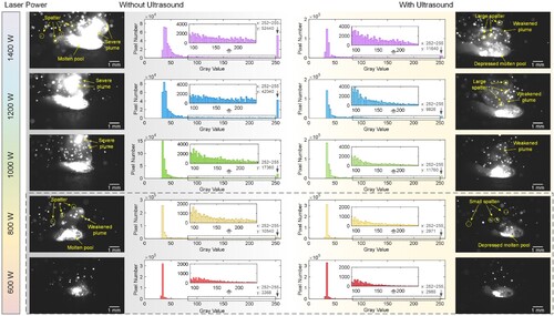
Figure 6. The extracted features from the melt pool, spatters and plume. (A–G) The area rate of the melt pool, spatter and plume was calculated in the study.

In Figure 4C, C is the starting point and the core point of the operational dataset. A1 and A2 are the border points of the operational dataset. And the radius size ϵ determined the size of the operational dataset. Thus, the X is defined as the dataset to be clustered in the study. The neighbourhood of a point x ∈ X within a given radius ϵ is called the ϵ-neighbourhood of x, denoted by N_ϵ. The mathematical representation of the N_ϵ is shown in Equation (1): (1) $N_{ϵ}\left(x\right)=\left\{y\in D|\mathrm{d}\mathrm{i}\mathrm{s}\mathrm{t}\mathrm{a}\mathrm{n}\mathrm{c}\mathrm{e}\left(x,y\right)\le ϵ,y\ne x\right\}$(1) (2) $\mathrm{d}\mathrm{i}\mathrm{s}\mathrm{t}\mathrm{a}\mathrm{n}\mathrm{c}\mathrm{e}\left(x,y\right)={\left(\sum _{i=1}^n{\left|x_i-y_i\right|}^2\right)}^{{\displaystyle \frac{1}{2}}}$(2) where the distance(x,y) is the Euclidean distance between x and y. D is the initial database.

And the following relationship is satisfied for the core point: |N_ϵ| ≥ Minpoints. Figure 6 shows the spatter a, b and c in preprocessed images and the corresponding spatter a′, b′ and c′ in raw images. To explore the effect of ultrasound and process parameters on spatters, the area ratio of the spatters can be further obtained in these images. 15 samples were randomly selected for statistical calculation under each process parameter. The specific analysis is presented in Section 5. Besides, the dynamic state of the plume and instability of the melt pool not only affected the formation of the spatter but also decreased the quality of the formed parts [5,7]. Therefore, the raw features of the plume and melt pool were also processed by the K-means++ method. Here, the clustering centre is K = 2. The distance between each observation and the c₁ was calculated in the paper, where the chosen observation is the first centroid, and is denoted c₁. The expression of selecting the next centroid c₂ at random from X with probability was obtained as follows (3) $P_2\left(x\right)=d^2\left(x_m,c_1\right)/\sum _{j=1}^n{d}^2\left(x_j,c_1\right)$(3) where the distance between c_j and the observation m was denoted as d(x_m, c_j). Furthermore, the centre j was chosen and the distances from each observation to each centroid were calculated. Similarly, the probability of selecting centroid j at random from X (4) $P_j\left(x\right)=d^2\left(x_m,c_p\right)/\sum _{\left\{h;x_h\in C_p\right\}}{d}^2\left(x_h,c_p\right)$(4) Among them, the m = 1, … ,n and p = 1, … ,j-1. C_p is the set of all observations closest to centroid c_p and x_m belongs to C_p. Finally, Equation (3) was repeated until K centroids are chosen. The distance metric d(x_m, c_j) was expressed as (5) $d\left(x,c\right)=1-x{c}^{\mathrm{\prime }}/\sqrt{\left(x{x}^{\mathrm{\prime }}\right)\left(c{c}^{\mathrm{\prime }}\right)}$(5) In Figure 6, the plume without ultrasound is quite severe when the laser power is at a high stage (such as P = 1400). The area ratio of the plume and melt pool reaches the range of 20%∼25%. However, the plume becomes weakened by using ultrasound during DED. Combined with the distribution of grey values in Figure 5, the pixel number in the range of grey values 252∼255 without ultrasound are higher than those of ultrasound. Similar results that ultrasonic vibration weakens the plume are obtained in the study. More formally, the proposed preprocessed method for melt pool and plume in raw images is summarised as follows.

Table

Algorithm 1: Preprocessing of melt pool and plume in the original images
Input: 1	image under each process parameter, S^q0^×^rdimension, q0 = qmelt pool + qplume, rdimension = 2.
Output:	Two clustered sets: Smelt pool, Splume.
Line 1:	A is all the vertical values (y) of the melt pool and the plume in the coordinate system,
Line 1:	Build an array B^1×^n0 = O,
Line 2:	for i1 = 1, 2, 3, … , n0
Line 3:	min(A) + (i1-1) × (max(A)-min(A))/n0 ≤ P < min(A) + (i1) × (max(A)-min(A))/n0
Line 4:	B(i) = NumberP
Line 6:	end for
Line 7:	Find all the Indexk in the B,
Line 8:	for k = 1, 2, 3, … , m0
Line 9:	if Indexk ≤ G×max(B)
Line 10:	C = [Indexk]
Line 11:	end if
Line 12:	end for
Line 13:	if IsEmpty($\mathit{C}$)  == false
Line 14	Temp1max = C(1);
Line 15	Temp2max = 1;
Line 16	Temp1this = C(1);
Line 17	Temp2this = 1;
Line 18	for ii = 1:(length(C) - 1)
Line 19	if C(ii + 1) - C(ii) >1
Line 20	%
Line 21	if Temp2max < Temp2this;
Line 22	Temp1max = Temp1this;
Line 23	Temp2max = Temp2this;
Line 24	%
Line 25	Temp1this = C(ii + 1);
Line 26	Temp2this = 1;
Line 27	end if
Line 28	else
Line 29	%
Line 30	Temp2this = Temp2this + 1;
Line 31	end for
Line 32	end if
Line 33	%
Line 34	if Temp2max < Temp2this;
Line 35	Temp1max = Temp1this;
Line 36	Temp2max = Temp2this;
Line 37	end if
Line 38	L = min(A) + (int(Temp1max + Temp2max /2)−1) × (max(A)-min(A))/n0
Line 39:	D = A – L;
Line 40:	D1′ =  (D1)^t1, D1 is the element of D < 0.
Line 41:	D2′ =  -(-D2)^t2, D2 is the element of D > 0.
Line 42:	Dnew = D;

4.2. Melt pool morphology, spatter and plume feature extraction

4.2.1. Principal component analysis (PCA)

Considering that the features extracted from the melt pool, plume and spatters may include some redundant information, principal component analysis (PCA) and auto-encoding were used for feature extraction to explore the effect of ultrasound and process parameters on the regions of interest (spatter, melt pool and plume) in the study, respectively. PCA based on the SVD (singular value decomposition) algorithm, as a feature selection scheme, can reduce the dimension of the analysed data by eliminating redundant data and irrelevant features, thereby improving the accuracy of feature extraction [26,50]. Firstly, the spatter, plume and melt pool as characteristic data were normalised with zero means. (6) $q={\displaystyle \frac{V-V_{\mathrm{m}\mathrm{i}\mathrm{d}}}{{\displaystyle \frac{1}{2}\left(V_{\mathrm{m}\mathrm{a}\mathrm{x}}-V_{\mathrm{m}\mathrm{i}\mathrm{n}}\right)}}}$(6) where V_min, V_mid and V_max are respectively the minimal, median and maximal values of the vector V. To obtain some valuable hidden information and weaken information, the SVD algorithm was used to separate the matrix data, the SVD of the matrix Q ∈ ℝ^n × m can be illustrated as follows. (7) $\mathit{Q}=\mathit{U}S{\mathit{V}}^{\mathrm{T}}$(7) The left eigenvector matrix U and right eigenvector matrix V are respectively an m × m orthogonal matrix and an n × n orthogonal matrix, and U^TU = E, V^TV = E. S is a m × n diagonal matrix, whose main diagonal elements are the singular value σ of the matrix Q sorting in descending order. The square of σ is equal to the eigenvalue λ of the matrix Q^TQ or QQ^T. (8) ${\mathit{S}}_{\lambda }=diag\left(\sqrt{{\lambda }_1},\sqrt{{\lambda }_2},\dots ,\sqrt{{\lambda }_r},\right),\sqrt{{\lambda }_1\ge }\sqrt{{\lambda }_2}\ge \dots \ge \sqrt{{\lambda }_r}$(8) where r is the rank of matrix Q, r ≤ min(m, n). Consequently, the matrix Q can be expressed as follows. (9) $\mathit{Q}=\sum _{k=1}^r{\sigma }_k{u}_k{v}_k^T$(9) where σ_k is the kth singular value of the matrix Q, which presents the coefficient of the eigenspace projection of the matrix Q and u_kv_k^T is the kth eigenspace. The matrix Q can be completely reconstructed. Thus, the local information can be reconstructed when selecting some eigenspaces, for example, the local melt pool, plume and spatters which are critical for forming quality.

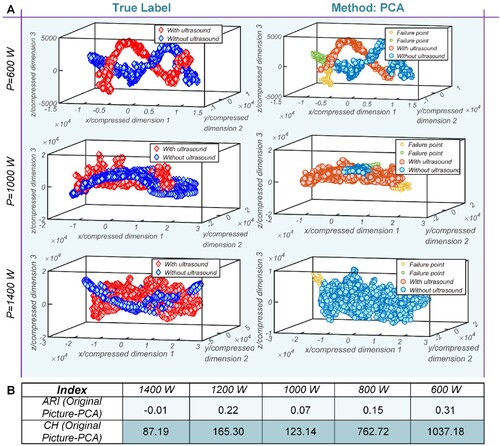
The compressed signals obtained by using PCA are displayed in Figure 7. The characteristic signals with ultrasound are marked in red. The signals without ultrasound are marked in blue. As can be seen from the true label, the spatial distribution of compressed signals in low power is smaller than those of high power. The non-ultrasound and ultrasound signals under low power are relatively concentrated in 3D spaces (i.e. P = 600 W). However, the signals under high power are sparsely distributed in relatively large spaces. (i.e. P = 1000, 1400 W). Meanwhile, in Figures 5 and 6, the same conclusions that the distributions of grey values and the features (spatters and plumes) are similar for ultrasound and non-ultrasound were concluded. It indicated that the plume and spatters under lower power are less impacted by ultrasound. In addition, compared to the true label, most of the non-ultrasound signals obtained by using the PCA method are correctly classified (i.e. P = 600, 1400 W), and only a few ultrasound signals are incorrectly classified in Figure 7(A) (i.e. P = 800 W). Thus, the non-ultrasound signals mixed with ultrasound signals are difficult to distinguish, which leads to difficulty in clustering. Some tolerable clustering error still exists in classification.

Figure 7. Compressed signals in 3D spaces by PCA.

4.2.2. Auto-encoding method

Considering that clustering algorithms based on PCA performed poorly, a designed auto-encoding with a fully connected network and a convolutional auto-encoding method were respectively proposed to analyse the dynamic melt pool feature, as shown in Figure 8A. Based on a previous study, the auto-encoder has the same network structure between input and output [51–53]. The auto-encoding method mainly consists of two stages: compressing original signals and reconstructing signals, as shown in Figure 8A. The encoding and decoding processes can be described: (10) $\mathit{h}=f\left(\mathit{x}\right)=s_f\left(\mathit{x}\ast \mathit{A}+\mathit{b}\right)$(10) (11) ${\mathit{x}}^{\mathrm{\prime }}=g\left(\mathit{h}\right)=s_h\left(\mathit{h}\ast \hat{\mathit{A}}+\mathit{c}\right)$(11) where A, b and Â, c are respectively the weight matrix and offset vector of the encoder and decoder, f(x) and g(h) denote the encoder and decoder's nonlinear activation function. To evaluate the performance of the proposed model, the reconstruction loss was obtained as follows: (12) $L\left(\mathit{x},{\mathit{x}}^{\mathrm{\prime }}\right)={\displaystyle \frac{1}{n}\sum ({\mathit{x}}_i^{\mathrm{\prime }}-{\mathit{x}}_i{)}^2}$(12) In the data processing stage, a large number of original signals were trained by unsupervised learning and acquired input representations of the input signal x in lower dimensions, further reconstructed these lower dimensional representations back to the higher dimensional data x′, aiming to make x and x′ as similar as possible. This method can reduce the reconstruction error between a reconstructed signal and an original signal by using an optimisation process based on gradient descent. The distribution of compressed signals showed some obvious features in 3D spaces when the reconstruction error was very small.

Figure 8. Schematic diagram of the auto-encoding model. (A) The model is a feed-forward network consisting of an auto-encoder and a decoder. (B) The detailed fully connected auto-encoders and the convolutional auto-encoders. In a fully connected network, the encoder takes a 1 × 496 × 832–sized input diffraction pattern image and puts it into a feature space via a series of fully connected layers (i.e. input 25,792 → 4567 → 543 → 98 → 23 → 3 latent space). The learning rate and the batch size are respectively 0.005 and 202. The decoding process is the reverse of the encoding process and the decoder adopts the same structure as the encoder. In a convolutional network, the encoder takes a 1 × 496 × 832–sized input diffraction pattern image and puts it into a feature space via a series of convolutional and max pooling layers (i.e. input 1 × 496 × 832 →1 × 98 × 165 → 7 × 18 × 32 → 130 × 1 × 1 → 3 × 1 × 1 → 3 × 24 × 41 → 2 × 123 × 209 → 1 × 495 × 839 → 1 × 496 × 832 latent space). Note that layers in the schematic are not drawn to scale. (C) The compressed signals obtained by the auto-encoding method are processed by DBSCAN.

For fully connected auto-encoders, a batch of train dataset H_h^m₁^×n₀ can be depicted as Equation (13), m₁ is the batch size. (13) $H_h^{m_1\times n_0}\subseteq U_i\left(H^{m_0\times n_0}\right),i=1,2,3\dots ,m_0=15,000,n_0=412672,m_1\le m_0$(13) Then, the compressed signal was transformed through multiple fully connected layers, and the reconstructed signal was obtained, as shown in Equation (14)-(18). (14) $H_h^{m_1\times n_0}=f_1\left(12\right)$(14) (15) $f_1\left(i+1\right)=\{\begin{array}{c}{f}_{2,i}\left[f_1\left(i\right)\cdot W_{i+1}^{n_i\times n_{i+1}}+B_{i+1}^{1\times n_{i+1}}\right],i>1\\ f_{2,i}\left(H_h^{m_1\times n_0}\cdot W_1^{n_0\times n_1}+B_1^{1\times n_1}\right),i=1\end{array}$(15) (16) $f_{2,i}\left(x\right)=\{\begin{array}{c}x,i=1,6,11\\ f_{3,i}\left(x\right),i=2,3,4,5,7,8,9,10\end{array}$(16) (17) $f_{3,i}\left(x\right)=\{\begin{array}{c}0,x<0\\ x,x\ge 0\end{array}$(17) (18) $\begin{array}{rl}& n_i=25792,4567,543,98,23,3,23,98,543,4567,\\ & 25792,412672,i=1,2,3,4,5,6,7,8,9,10,11,12\end{array}$(18) where W_i + 1 and B_i + 1 are respectively the weight matrix and offset vector of a dense layer. Likewise, the reconstructed signal acquired by convolutional auto-encoders can be expressed as Equation (19). 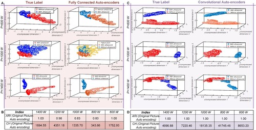(19) $f\left(i,j\right)=\left(X\ast W\right)\left(i,j\right)=\sum _m\sum _{n}x\left(i+m,j+n\right)w\left(m,n\right)$(19) As shown in Figure 8B, the specific frameworks of fully connected auto-encoders and convolutional auto-encoders are illustrated. In the designed network, 1500 images in each case are used in the study. The results of the distribution of compressed signals obtained by the auto-encoding algorithm are shown in Figure 9. Considering that the dynamic characteristics of the spatter, melt pool and plume were changed by ultrasound, the compressed signals were obviously divided into two clustering areas. All signals under different cases were respectively marked in red and blue. The clustering of compressed signals by fully connected auto-encoders and convolutional auto-encoders is consistent with those of true labels. If only based on the PCA method, some isolated areas refer to points clustered as noise. And the density of a non-ultrasound-points set and an ultrasound-points set is similar in some areas. For example, the density of the area is similar when the power is 1400 W in Figure 7. It indicated that the clustering obtained based on PCA was not excellent. However, based on designed auto-encoding, clustering errors caused by noise signals are reduced, resulting in obvious differences between ultrasound and non-ultrasound features.

Figure 9. Compressed signals in 3D spaces by the fully connected auto-encoders and the convolutional auto-encoders.

5. Results and discussion

5.1. Evaluation criteria on the performance of the supposed unsupervised learning

Considering that true labels of the sample can be obtained, several criteria are used to evaluate the performance of an algorithm in a typical supervised method, i.e. accuracy, precision, sensitivity (recall) and specificity. Internal evaluation and external evaluation are two main aspects to verify the clustering effects. Specifically, purity, rand index (RI), F-score, adjusted rand index (ARI) and the Calinski-Harbasz (CH) score can be used to evaluate the performance of an algorithm in a typical cluster analysis. These criteria can evaluate the differences among several clusters and the similarity among elements within a cluster. Here, considering the characteristics of the melt pool, plume and spatters, the ARI and CH score is used to analyse the performance of the clustering algorithm proposed in the study. The ARI and CH score are respectively described as Equation (20), Equations (21)–(23) (20) $\mathrm{A}\mathrm{R}\mathrm{I}={\displaystyle \frac{\mathrm{R}\mathrm{I}-\mathrm{E}\mathrm{x}\mathrm{p}\mathrm{e}\mathrm{c}\mathrm{t}\mathrm{e}\mathrm{d}\left(\mathrm{R}\mathrm{I}\right)}{max\left(\mathrm{R}\mathrm{I}\right)-\mathrm{E}\mathrm{x}\mathrm{p}\mathrm{e}\mathrm{c}\mathrm{t}\mathrm{e}\mathrm{d}\left(\mathrm{R}\mathrm{I}\right)}}$(20) (21) $S\left(K\right)={\displaystyle \frac{S{S}_B}{k-1}/{\displaystyle \frac{S{S}_W}{N-k}={\displaystyle \frac{tr\left(B_k\right)}{tr\left(W_k\right)}\times {\displaystyle \frac{N-k}{k-1}}}}}$(21) (22) $W_k=\sum _{q=1}^k\sum _{x\in C_q}\left(x-c_q\right)(x-c_q{)}^T$(22) (23) $B_k=\sum _{q=1}^k{n}_q\left(c_q-c_E\right)(c_q-c_E{)}^T$(23) where RI is the rand index, RI∈[0,1]. Thus, the value range of ARI is [−1,1], and the clustering result is better when the value of ARI is larger. In Figure 7, the values of ARI by PCA method are respectively 0.31, 0.15, 0.07, 0.22, −0.01 when the laser power takes the values of 1400, 1200, 1000, 800, 600 W, respectively. However, the values of ARI by the designed auto-encoding method are approximately 1 under different laser power, as shown in Figure 9. It indicated that the feature extraction of the melt pool, spatters and plume by the designed auto-encoding method was better than those of the PCA method. The value of ARI for convolutional auto-encoders is more stable than that of fully connected auto-encoders. In addition to evaluating the differences among several clusters, the CH score was adopted in the analysis of the similarity among elements within a cluster. In Equations (22) and (23), k, N, SS_B and SS_W respectively represent the number of clustering categories, the number of all data, the inter-class variance and the intra-class variance. W_k and B_k are within-cluster dispersion and between-clusters dispersion means. Besides, n_q, c_q, c_E and C_q are the total number of data points of class q, the centroid of the class q, the centroid of all data and the set of all data in the class q, respectively. And the higher CH score indicates the better clustering effect of the used method. From the calculated CH scores, the CH scores by using the designed auto-encoding method are significantly higher than those of the PCA method. For example, the CH score is 1335.70 by auto-encoding method when the laser power is 1000 W. However, the CH score is only 74.05 by PCA.

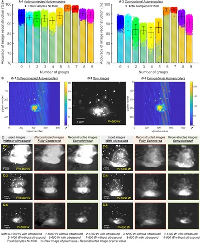
Furthermore, the accuracy of reconstructed images and absolution error of pixel points are calculated for fully connected networks and convolution networks. As shown in Figure 10 and Supplementary Figure S4, the average accuracy of reconstructed images by fully connected auto-encoder and convolution auto-encoder is respectively 94.52% and 90.05% under 10 cases. There is good agreement between the raw images and reconstructed images in terms of the characteristics of the melt pool and plume by convolutional auto-encoders and fully connected auto-encoders. The same conclusions are drawn by the absolute error distribution map of pixel points per image in Figure 10B. Thus, it stated the designed fully connected auto-encoders and convolutional auto-encoders in feature extraction and reconstruction image were effective in monitoring the feature of the melt pool during metal 3D printing.

Figure 10. Image feature reconstruction error analysis. (A) Accuracy of image reconstruction for the fully connected auto-encoders and the convolutional auto-encoders in different cases. (B) The absolute error of original image pixels and reconstructed image pixels. (C) Reconstructed images by the fully connected auto-encoders and the convolutional auto-encoders.

5.2. The results of monitoring the melt pool, spatters and plume

The dynamic characteristics of the melt pool, spatters and plumes are analysed in Figures 5 and 6. Regardless of non-ultrasound and ultrasound, both the area of the plume and the number of splatters increase significantly with the increase of laser power (i.e. increasing energy density). The reason is that the energy input exceeds a certain threshold and the metal vapour inside the keyhole of the melt pool transitions from a steady flow to a chaotic flow, resulting in a change in the refractive index of the vapour and aggravating the plume phenomenon. In addition, serious plume during DED also affects the forming quality of the melt track after solidification and defects [53–57]. In Figure 11A,B, the depth of tracks was increased due to the increase in energy density. The transition surface between the substrate and cladding layer also appears uneven in the cross-section of tracks compared to the low energy density. Moreover, the effect of other process parameters (laser power, scanning rate and powder flow rate) on the size of melt tracks is shown in Figure 11D. Consequently, the decrease in the scanning rate and the increase in the laser power both cause an increase in the laser density, which further leads to the increase in the depth and width of melt tracks. However, the effect of the powder flow rate on the depth of tracks was weaks. The width was slightly increased because of the increase in powder flow rate.

Figure 11. Morphologies of the solidified tracks and microstructure under different conditions. (A) Morphologies in the cross-section of the solidified tracks during DED and UADED. (B) Effect of energy density on the track width (w₁) and track depth (d₁). (C) The top surface defects of solidified tracks during DED and UADED. (D) Effect of processing parameters (laser power, scanning rate and powder flow rate) on the track width (w₁) and track depth (d₁). (E) and (F) Microstructure and grain size distribution during DED and UADED.

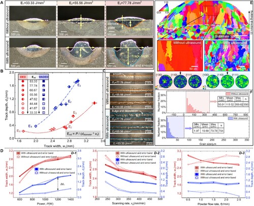
Different from DED, the area of the plume is reduced during UADED due to the application of ultrasound, as shown in Figure 6. In UADED, the flow pattern of the melt pool was dominated by the ultrasound-induced inertial force [7]. The inertial force drives the melt pool to flow back and forth along the scanning direction. There is no significant Marangoni during UADED. The flow stable state was disrupted due to the ultrasound. More profoundly, the flow of melt vapour inside the keyhole can become chaotic and weaken the generation of plumes. And the weak phenomena are obvious when the laser power is increased. The surface of the dynamic melt pool was depressed because the flow mode was changed, along with fish-scale ripples. However, it can be seen that the fraction of spatter during UADED is much more than that of DED. The average fraction in UADED is 1.20% when the laser power is 1400 W. The reason is that the inertial force drives the melt pool material to be thrown out to form spatters. The spatters of the formation mechanism are different from the conventional DED. As a result, the surface of melt tracks appears bulged and depressed in Figure 11C and supplementary Figure S5. Specifically, the bulge and depression are quite serious when the energy density is up to 77.78 J/mm². In the cross-section of melt tracks, the depth of tracks is significantly increased in UADED with the increase of the energy density, as shown in Figure 11A. Additionally, characteristic changes of the melt pool, spatter and plume also affect the microstructure and orientation of the samples. In Figure 11E,F, the sample manufactured without ultrasound exhibits columnar primary γ grains of 113.52 μm in average size. For the sample fabricated with ultrasound, the average grain size is only 10.89 μm due to cavitation and acoustic streaming by ultrasound, with a near-random crystallographic texture.

6. Conclusion

In this paper, a hybrid unsupervised method was proposed to distinguish the feature differences (spatter, plume, etc.) between ultrasound and non-ultrasound, and further to diagnose the print quality. First, a high-speed camera was used to monitor the printing process in real time, and then the captured raw sequential images were processed by the hybrid clustering algorithm, where the characteristics of the melt pool, plume and spatters were extracted. The area ratio of plume and spatters was quantified and the clustering performance for the DED and UADED was discussed. Finally, the quality of as-printed tracks and the microstructure features was also investigated. The detailed conclusions are as follows:

• o For the dynamic characteristics, the area fraction of the plume generated during DED is serious compared to UADED: the area fraction of the former reaches 21.53% when the laser power is 1400 W, while it is only 7.99% for the latter. The flow pattern was changed in UADED as the inertial force drives the melt pool to flow back and forth along the scanning direction and there is no significant Marangoni. Due to the ultrasound, the influence of weakening the plume is more pronounced with the laser power increasing during UADED. Moreover, the depression with fish scale appeared on the surface of the melt pool and the area fraction of spatter also obviously increased compared to the DED.

• o In terms of feature extraction, the designed auto-encoding method (fully connected and convolutional auto-encoders) can effectively discriminate the differences between DED and UADED in the melt pool characteristics, plume and spatter. Compared with those of PCA, the evaluation criteria of the auto-encoding method are more accurate and the clustering effects are relatively robust in feature extraction. Concerning ARI, the value is 1 by the fully connected auto-encoders when the laser power is 1400 W, while the value is only −0.01 by PCA. And the CH score of the auto-encoding method is higher than that of PCA. In addition, the fully-connected auto-encoder owns a better average accuracy for image reconstruction than the convolution auto-encoder, among the 10 cases, their corresponding results are 94.52% and 90.05%, respectively.

• o The experimental validations demonstrated that the ultrasound could weaken the formation of keyholes from the cross-section of melt tracks. Compared to DED, the depth of the tracks is greater during UADED since the flow mode of the melt pool is changed into reciprocal flow mode by introducing ultrasound. For the microstructures, the sample printed without ultrasound exhibits large columnar primary γ grains with an average size of 113.52 μm. By contrast, the average grain size is only 10.89 μm for UADED and a near-random crystallographic texture is generated. These can be attributed to the cavitation and acoustic streaming by ultrasound.

In conclusion, the quantitative analysis and the reliable validation suggest that the designed fully connected auto-encoders and convolutional auto-encoders are effective in feature extraction and image reconstruction. The proposed methods can provide a robust theoretical basis to understand the physical phenomena during DED and UADED more deeply and to guide to match the optimum process parameters for reducing potential defects and improving print quality.

Disclosure statement

No potential conflict of interest was reported by the author(s).

Additional information

Funding

This work was funded by the National Natural Science Foundation of China (51975112); Fundamental Research Funds for Central Universities (N2203011); and Liao Ning Revitalization Talents Program (XLYC1807063). Liaoning Revitalization Talents Program

References

- Cadiou S, Courtois M, Carin M, et al. 3D heat transfer, fluid flow and electromagnetic model for cold metal transfer wire arc additive manufacturing (Cmt-Waam). Additive Manuf. 2020;36:101541. doi:10.1016/j.addma.2020.101541
- Hu Y. Recent progress in field-assisted additive manufacturing: materials, methodologies, and applications. Mater Horiz. 2021;8(3):885–911. doi:10.1039/D0MH01322F
- Wang S, Ning J, Zhu L, et al. Role of porosity defects in metal 3D printing: formation mechanisms, impacts on properties and mitigation strategies. Mater Today. 2022;59(October):133–160. doi:10.1016/j.mattod.2022.08.014
- Todaro CJ, Easton MA, Qiu D, et al. Grain refinement of stainless steel in ultrasound-assisted additive manufacturing. Additive Manuf. 2021;37(September 2020):101632. doi:10.1016/j.addma.2020.101632
- Todaro CJ, Easton MA, Qiu D, et al. Grain structure control during metal 3D printing by high-intensity ultrasound. Nat Commun. 2020;11(1):1–9. doi:10.1038/s41467-019-13874-z
- Yuan T, Kou S, Luo Z. Grain refining by ultrasonic stirring of the weld pool. Acta Mater. 2016;106:144–154. doi:10.1016/j.actamat.2016.01.016
- Yang Z, Wang S, Zhu L, et al. Manipulating molten pool dynamics during metal 3D printing by ultrasound. Appl Phys Rev. 2022;9(2). doi:10.1063/5.0082461
- Yang Z, Zhu L, Zhang G, et al. Review of ultrasonic vibration-assisted machining in advanced materials. Int J Mach Tools Manuf. 2020;156(June):103594. doi:10.1016/j.ijmachtools.2020.103594
- Wang S, Guo ZP, Zhang XP, et al. On the mechanism of dendritic fragmentation by ultrasound induced cavitation. Ultrason Sonochem. 2019;51(October 2018):160–165. doi:10.1016/j.ultsonch.2018.10.031
- Wang S, Kang J, Guo Z, et al. In situ high speed imaging study and modelling of the fatigue fragmentation of dendritic structures in ultrasonic fields. Acta Mater. 2019;165:388–397. doi:10.1016/j.actamat.2018.11.053
- Cong W, Ning F. A fundamental investigation on ultrasonic vibration-assisted laser engineered net shaping of stainless steel. Int J Mach Tools Manuf. 2017;121(February):61–69. doi:10.1016/j.ijmachtools.2017.04.008
- Ning F, Hu Y, Liu Z, et al. Ultrasonic vibration-assisted laser engineered net shaping of Inconel 718 parts: a feasibility study. Procedia Manuf. 2017;10:771–778. doi:10.1016/j.promfg.2017.07.074
- Wang H, Hu Y, Ning F, et al. Ultrasonic vibration-assisted laser engineered net shaping of Inconel 718 parts: effects of ultrasonic frequency on microstructural and mechanical properties. J Mater Process Technol. 2020;276(April 2019):116395. doi:10.1016/j.jmatprotec.2019.116395
- Yang Z, Zhu L, Wang S, et al. Effects of ultrasound on multilayer forming mechanism of Inconel 718 in directed energy deposition. Additive Manuf. 2021;48:102462. doi:10.1016/j.addma.2021.102462
- Yang Z, Zhu L, Ning J, et al. Revealing the influence of ultrasound/heat treatment on microstructure evolution and tensile failure behavior in 3D-printing of Inconel 718. J Mater Process Technol. 2022;305(March):117574. doi:10.1016/j.jmatprotec.2022.117574
- Grasso M, Laguzza V, Semeraro Q, et al. In-process monitoring of selective laser melting: spatial detection of defects Via image data analysis. J Manuf Sci Eng, Transactions of the ASME. 2017;139(5). doi:10.1115/1.4034715
- Fernandez A, Souto A, Gonzalez C, et al. Embedded vision system for monitoring Arc welding with thermal imaging and deep learning. 2020 International Conference on Omni-Layer Intelligent Systems, COINS 2020; 2020. doi:10.1109/COINS49042.2020.9191650
- Huang W, Kovacevic R. Noise reduction during acoustic monitoring of laser welding of high-strength steels. Proceedings of the ASME International Manufacturing Science and Engineering Conference. MSEC2009-84080; 2009. 1–8.
- Ramalho A, Santos TG, Bevans B, et al. Effect of contaminations on the acoustic emissions during wire and Arc additive manufacturing of 316L stainless steel. Additive Manuf. 2022;51(September 2021):102585. doi:10.1016/j.addma.2021.102585
- Meng L, McWilliams B, Jarosinski W, et al. Machine learning in additive manufacturing: a review. Jom. 2020;72(6):2363–2377. doi:10.1007/s11837-020-04155-y
- Sing SL, Kuo CN, Shih CT, et al. Perspectives of using machine learning in laser powder bed fusion for metal additive manufacturing. Virtual Phys Prototyp. 2021;16(3):372–386. doi:10.1080/17452759.2021.1944229
- Lin X, Zhu K, Hsi Fuh JY, et al. Metal-based additive manufacturing condition monitoring methods: from measurement to control. ISA Trans. 2022;120:147–166. doi:10.1016/j.isatra.2021.03.001
- Yang S, Huang W, Lin D, et al. Monitoring of the spatter formation in laser welding of galvanized steels. Proceedings of the 2008 International Manufacturing Science and Engineering Conference. Msec _ Icmp2008-72224. 1–4; 2008.
- Zhang W, Ma H, Zhang Q, et al. Prediction of powder Bed thickness by spatter detection from coaxial optical images in selective laser melting of 316L stainless steel. Mater Des. 2022;213:110301. doi:10.1016/j.matdes.2021.110301
- Ye D, Zhu K, Hsi Fuh JY, et al. The investigation of plume and spatter signatures on melted states in selective laser melting. Opt Laser Technol. 2019;111(March 2018):395–406. doi:10.1016/j.optlastec.2018.10.019
- Zhang Y, Hong GS, Ye D, et al. Extraction and evaluation of melt pool, plume and spatter information for powder-bed fusion AM process monitoring. Mater Des. 2018;156:458–469. doi:10.1016/j.matdes.2018.07.002
- Zhang, Yingjie, Hong Geok Soon, Dongsen Ye, Jerry Ying Hsi Fuh, and Kunpeng Zhu. 2020. Powder-bed fusion process monitoring by machine vision with hybrid convolutional neural networks. IEEE Trans Ind Inf 16 (9). 5769–5779. doi:10.1109/TII.2019.2956078.
- Grasso M, Demir AG, Previtali B, et al. In situ monitoring of selective laser melting of zinc powder via infrared imaging of the process plume. Robot Comput Integr Manuf. 2018;49(July 2017):229–239. doi:10.1016/j.rcim.2017.07.001
- Yang Z, Lu Y, Yeung H, et al. From scan strategy to melt pool prediction: a neighboring-effect modeling method. J Comput Inf Sci Eng. 2020;20(5). doi:10.1115/1.4046335
- Fathizadan S, Ju F, Lu Y. Deep representation learning for process variation management in laser powder bed fusion. Additive Manuf. 2021;42(November 2020):101961, doi:10.1016/j.addma.2021.101961
- Kim J, Yang Z, Ko H, et al. Deep learning-based data registration of melt-pool-monitoring images for laser powder bed fusion additive manufacturing. J Manuf Syst. 2023;68(March):117–129. doi:10.1016/j.jmsy.2023.03.006
- Khanzadeh M, Chowdhury S, Tschopp MA, et al. In-situ monitoring of melt pool images for porosity prediction in directed energy deposition processes. IISE Trans. 2019;51(5):437–455. doi:10.1080/24725854.2017.1417656
- Khanzadeh M, Bian L, Shamsaei N, et al. Porosity detection of laser based additive manufacturing using melt pool morphology clustering. Solid Freeform Fabrication 2016: Proceedings of the 27th Annual International Solid Freeform Fabrication Symposium - An Additive Manufacturing Conference, SFF 2016, no. November: 1487–1494; 2016.
- Ko H, Lu Y, Yang Z, et al. A framework driven by physics-guided machine learning for process-structure-property causal analytics in additive manufacturing. J Manuf Syst. 2023;67(February):213–228. doi:10.1016/j.jmsy.2022.09.010
- You D, Gao X, Katayama S. Monitoring of high-power laser welding using high-speed photographing and image processing. Mech Syst Signal Process. 2014;49(1–2):39–52. doi:10.1016/j.ymssp.2013.10.024
- Meng W, Yin X, Fang J, et al. Dynamic features of plasma plume and molten pool in laser lap welding based on image monitoring and processing techniques. Opt Laser Technol. 2019;109(October 2017):168–177. doi:10.1016/j.optlastec.2018.07.073
- Tan Z, Fang Q, Li H, et al. Neural network based image segmentation for spatter extraction during laser-based powder bed fusion processing. Opt Laser Technol. 2020;130(March):106347. doi:10.1016/j.optlastec.2020.106347
- Fang Q, Tan Z, Li H, et al. In-situ capture of melt pool signature in selective laser melting using U-net-based convolutional neural network. J Manuf Process. 2021;68(PA):347–355. doi:10.1016/j.jmapro.2021.05.052
- Criales LE, Arısoy YM, Lane B, et al. Laser powder bed fusion of nickel alloy 625: experimental investigations of effects of process parameters on melt pool size and shape with spatter analysis. Int J Mach Tools Manuf. 2017;121(March):22–36. doi:10.1016/j.ijmachtools.2017.03.004
- Repossini G, Laguzza V, Grasso M, et al. On the use of spatter signature for In-situ monitoring of laser powder bed fusion. Additive Manuf. 2017;16:35–48. doi:10.1016/j.addma.2017.05.004
- Baumgartl H, Tomas J, Buettner R, et al. A deep learning-based model for defect detection in laser-powder Bed fusion using in-situ thermographic monitoring. Prog Additive Manuf. 2020;5(3):277–285. doi:10.1007/s40964-019-00108-3
- Chebil G, Bettebghor D, Renollet Y, et al. Deep learning object detection for optical monitoring of spatters in L-PBF. J Mater Process Technol. 2023;319(March):118063. doi:10.1016/j.jmatprotec.2023.118063
- Hagenlocher C, O’Toole P, Xu W, et al. In process monitoring of the thermal profile during solidification in laser directed energy deposition of aluminium. SSRN Electron J. 2022: 100084. doi:10.2139/ssrn.4098269
- Li J, Liu Y, Tao Y, et al. Analysis of vapor plume and keyhole dynamics in laser welding stainless steel with beam oscillation. Infrared Phys Technol. 2021;113(2):103536. doi:10.1016/j.infrared.2020.103536
- Jakumeit J, Zheng G, Laqua R, et al. Modelling the complex evaporated gas flow and Its impact on particle spattering during laser powder bed fusion. Additive Manuf. 2021;47(December 2020):102332. doi:10.1016/j.addma.2021.102332
- Zhang Y, You D, Gao X, et al. Online monitoring of welding status based on a DBN model during laser welding. Engineering. 2019;5(4):671–678. doi:10.1016/j.eng.2019.01.016
- Matthews MJ, Guss G, Khairallah SA, et al. Denudation of metal powder layers in laser powder bed fusion processes. Acta Mater. 2016;114:33–42. doi:10.1016/j.actamat.2016.05.017
- Ly S, Rubenchik AM, Khairallah SA, et al. Metal vapor micro-jet controls material redistribution in laser powder bed fusion additive manufacturing. Sci Rep. 2017;7(1):1–12. doi:10.1038/s41598-016-0028-x
- Liu J, Wen P. Metal vaporization and its influence during laser powder bed fusion process. Mater Des. 2022;215:110505. doi:10.1016/j.matdes.2022.110505
- Chen YQ, Zhao BN, Chen C, et al. Identification of ore-finding targets using the anomaly components of ore-forming element associations extracted by SVD and PCA in the Jiaodong Gold Cluster Area, Eastern CHINA. Ore Geol Rev. 2022;144(November 2021):104866. doi:10.1016/j.oregeorev.2022.104866
- Lin X, Wang Q, Hsi Fuh JY, et al. Motion feature based melt pool monitoring for selective laser melting process. J Mater Process Technol. 2022;303(February):117523. doi:10.1016/j.jmatprotec.2022.117523
- Lou S, Deng J, Lyu S. Chaotic signal denoising based on simplified convolutional denoising auto-encoder. Chaos, Solitons Fractals. 2022;161:112333. doi:10.1016/j.chaos.2022.112333
- Chan H, Nashed YSG, Kandel S, et al. Rapid 3D nanoscale coherent imaging via physics-aware deep learning. Appl Phys Rev. 2021;8(2). doi:10.1063/5.0031486
- Yang Y, Gao Z, Cao L. Identifying optimal process parameters in deep penetration laser welding by adopting hierarchical-kriging model. Infrared Phys Technol. 2018;92(November 2017):443–453. doi:10.1016/j.infrared.2018.07.006
- Bitharas I, Parab N, Zhao C, et al. The interplay between vapour, liquid, and solid phases in laser powder bed fusion. Nat Commun. 2022;13(1):1–12. doi:10.1038/s41467-022-30667-z
- Panwisawas C, Perumal B, Ward RM, et al. Keyhole formation and thermal fluid flow-induced porosity during laser fusion welding in titanium alloys: experimental and modelling. Acta Mater. 2017;126(June 2021):251–263. doi:10.1016/j.actamat.2016.12.062
- Li Y, Tian S, Wu CS, et al. Experimental sensing of molten flow velocity, weld pool and keyhole geometries in ultrasonic-assisted plasma Arc welding. J Manuf Process. 2021;64(March):1412–1419. doi:10.1016/j.jmapro.2021.03.005