Modelling and researching the evolution of stress during arc-directed energy deposition (ADED) hybrid inter-layer hammering

ABSTRACT

Hybrid manufacturing of arc-directed energy deposition (ADED) and inter-layer hammering can build components with low detrimental residual stress (RS) and warping. Inter-layer hammering with lower load demand has proved to be a promising technology to improve the microstructure and mechanical properties. In this paper, a finite element model of the ADED hybrid inter-layer hammering was constructed for the first time. The accuracy of the model is evaluated by comparing thermal history, RS, and warping. The results show that the maximum compressive RS -25Mpa appears at 3 mm from the top of the wall after a single inter-layer hammering. The RS of the inspection position is reduced by 74.6% after six layers of hammering compared with the wall manufactured by ADED alone, and low-stress distribution with a value of -30Mpa appears in the range of 7 mm to 15 mm from the substrate surface. The warping of the wall in the building direction was completely suppressed (from 0.21 mm to 0 mm). In addition, the plastic strain introduced by the hammering at the wall top exacerbates the “misfit” between the regions of the wall top, resulting in tensile stress at the wall top.

KEYWORDS:

• Arc-directed energy deposition
• inter-layer hammering
• finite element analysis
• residual stress
• hybrid manufacturing

1. Introduction

Arc-directed energy deposition (ADED), a new near-net forming directed energy deposition process layer by layer, can meet the requirements of small batches and personalised manufacturing. It imposes no special demands on equipment, and standard welding equipment, and consumables can be adopted, which significantly reduces operating costs [1]. A significant amount of energy is rapidly released during the ADED process, resulting in RS and severe deformation that hinder its application in large-part manufacturing. Numerous techniques have been developed to mitigate these effects, which can be broadly categorised into two groups [2]. A set of techniques relies on optimising the deposition parameters and sequences to mitigate residual stress (RS) and deformation levels. According to related reports, Brust et al. [3] studied the effect of deposition sequence on the RS of deposition parts by finite element analysis. The results show that the optimal deposition sequence can effectively control the deformation, but the mitigation was affected by the part structure studied. Mughal et al. [4] used finite element analysis to investigate the best deposition sequences of a square with seven parallel welds. The results show that the best deposition sequences were from the external path to the end of the central path. This method has gradually evolved to find optimal parameters and deposition sequences utilising intelligent algorithms. The method of reducing RS by optimising deposition parameters and sequence has shifted to finding the best deposition parameters and sequence by algorithms. Chigilipalli et al. [5], use neuro-fuzzy modelling to ascertain metal deposition parameters for wire arc additive manufacturing. Sun et al. [6], created a deposition model based on head sequence-driven residual stress reduction in additive manufacturing.

Another primary approach for reducing RS is through the implementation of additional auxiliary processes. This method can be categorised into two types: post-deposition treatment and inter-layer auxiliary processes. Post-deposition treatment includes post-deposition rolling [7], post-deposition hammering and post-deposition heat treatment [8,9], etc. Post-deposition heat treatment releases RS in the part by placing it in a high-temperature environment for a period of time. Hongyao et al. [8] successfully reduced the RS of the ADED part by using induction heat treatment, and the predicted results were in a certain agreement with the experimental results. Goviazin et al. [9] studied the effect of post-deposition heat treatment on the RS of 316 L stainless steel parts and found that the RS was almost completely eliminated under the heat treatment condition of 600°C. Post-deposition rolling and post-deposition hammering are to introduce plastic deformation to alleviate the deformation of parts during the ADED process after the ADED process, and to reduce the RS in the part generated by ADED. Colegrove et al. [10] studied the effects of load, different roller types, and friction on RS reduction of the ADED parts during post-deposition rolling. It is found that a high load can effectively reduce the tensile RS of the parts. Due to the limitation of rolling depth, the reduction effect of tensile RS is weak in the deeper region. However, the mitigation effect of post-deposition treatment was limited by the influence of depth and only mitigated the stress within a distance from the top of the wall. The post-deposition treatment way is weak in mitigating RS during the deposition of large parts [7]. It should be noted that parts may fail prematurely due to excessive deformation or cracks before post-deposition treatment. On the contrary, the advantage of the inter-layer auxiliary process is that the RS of the ADED parts can be reduced in situ and more effectively and timely during the deposition. Inter-layer rolling was recognised as an inter-layer auxiliary process that can effectively mitigate part RS. Martina et al. [11] studied the effect of the inter-layer rolling process on reducing the RS of ADED parts. Compared with the wall fabricated by ADED alone, the stress and deformation of the wall fabricated by ADED hybrid inter-layer rolling are reduced by 60% and more than 50%. Colegrove et al.[12] studied the effect of inter-layer rolling on the residual stress of titanium ADED wall. The result show that the peak tensile stress of the ADED wall is significantly reduced and the deformation of the wall is reduced by half compared with the control group.

Finite element analysis (FEA) is a robust method for studying manufacturing processes, which can significantly reduce the amount of experimental work. At present, scholars at Cranfield University have successfully applied the FEA to the rolling analysis. Gornyakov et al. [7] used ABAQUS software to construct a finite element model of post-deposition rolling based on the research of Colegrove et al. [10]. Studying the effects of load, different types of rolls, and friction on reducing RS of ADED parts. It is found that a high load can effectively reduce the tensile RS of parts. Due to the limitation of the influence depth, the tensile RS reduction effect is weak for the region with a deeper position. Similarly, Abbaszadeh et al. [13] simulated rolling of WAAM walls using the finite element method (FEM) software ABAQUS/Standard. Studying the effects of rolling load and roll radius on the RS field and plastic strain distribution of an ADED wall with different materials. Gornyakov et al. [14] established four efficient models for calculating the rolling process and applied them to a short transient rolling model, which reduced the calculation time by 96.9% compared to the control model. Gornyakov et al. [15] developed a finite element model of ADED hybrid inter-layer rolling based on the solution mapping of the ABAQUS software and the efficient computing model of previous research [14]. The interaction between the ADED process and the inter-layer rolling process is studied and the inter-layer rolling strategy is optimised according to the prediction results of the model. It is best to reduce the RS of the ADED wall by using a slotted roller with every four layers of deposition. Tangestani et al [16] studied the influence of roller curvature depth and roller shape on the RS and deformation of the ADED part in lateral clamping rolling by finite element analysis. It was found that the RS distribution was sensitive to the rolling direction. Using a thicker roller to apply fewer rolling passes can generate more compressive RS on the ADED wall.

However, rolling equipment was complex and required a high load as a power source during operation, and rolling with a flat roller requires lubrication and degreasing of the rolls. These operations significantly increase production time and energy consumption [15]. Lateral clamping rolling has the problem of insufficient improvement depth in the direction perpendicular to the ADED wall, and it was not applicable for multi-deposition layer interval distribution structures. Compared with inter-layer rolling, inter-layer hammering equipment was simple and flexible, only compressed air is used as a power source to complete the work in a short time. Currently, the research on inter-layer hammering primarily focuses on its impact on the microstructure and properties [17] of ADED walls. However, the effects of inter-layer hammering on RS and warping of the ADED wall have not been studied.

This study evaluates the ADED hybrid inter-layer hammering process and presents two challenges in constructing the inter-layer hammering hybrid ADED finite element model (Hybrid model). One is to determine how to transfer the calculation results of the ADED process and hammering process, including stress, strain, deformation, and temperature field. The other is to determine how the new layers are added during the new ADED process. The ‘field circulation transfer’, a technology used to transfer calculation results between deposition and hammering models, and the ‘surface mesh extraction and reconstruction’, a modelling method that guarantees cyclic calculation of the hybrid model proposed to solve these two challenges. The mitigation effect and influence range of inter-layer hammering on stress and deformation of ADED walls are studied based on the hybrid model. An interaction theory is proposed to better understand the evolution characteristics of stress in ADED walls during the hybrid process. This study guides optimising the ADED hybrid inter-layer hammering process to mitigate the accumulation of RS and warping more effectively.

2. Materials and methods

2.1. Material properties

The weldability of materials is a crucial factor in determining the suitability of metals and their alloys for ADED. Commonly used materials for part construction include steel [18], titanium alloy [19], aluminum alloy [20], and nickel superalloy [21], among others. The 5B06 aluminum alloy is primarily composed of magnesium. This alloy boasts exceptional heat resistance, welding performance, and fatigue strength. The aluminum alloy of 5B06 cannot be strengthened by heat treatment, but it can mitigate the strength by cold working [17]. In this study, 5B06 aluminum alloy was selected as the welding wire and substrate materials. The element composition of 5b06 is shown in Table 1. The material parameters involved in the hybrid model are computed using the Simufact Material library®. The mechanical and thermophysical parameters of materials used in the hybrid model are shown in Figure 1.

Figure 1. Material parameter, (a) Mechanical parameter, (b) Thermophysical parameter.

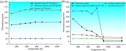
Table 1. Chemical compositions of the wire-deposited metal and the substrate (wt %).

Al	Mg	Mn	Cr	Cu	Fe	Si	Ti	Zn
91.6–93.7	4.5–5.6	0.1∼0.6	0.2	0.1	0.5	0.4	0.2	0.2

The cold forging model provided by Simufact® was used for describing the hardening of the materials during the hybrid process. The cold forging model mainly considers the effect of strain on the yield stress of materials, it can be used to describe the strain-strengthening behaviour between yield and necking initiation. The relationship between the stress and strain of the material in the hybrid process follows the cold forging formula (1) [22], where ‘$\phi$’ is the strain, N is the strain hardening exponent, and the value is 0.13 [22]. ‘C’ is the yield limit at room temperature. (1) ${\sigma }_F=C{\phi }^N$(1)

2.2. Experiment

Figure 2a, b show the utilisation of two six-degree-of-freedom welding arms as carriers for ADED and hammering. During the ADED process, a welding machine with a cold metal transfer (CMT) work pattern serves as the energy source, connected to a mechanical arm, and working in conjunction with the wire feeder. Two ADED wall specimens were prepared. One specimen, referred to as group 1, was prepared by ADED hybrid inter-layer hammering. The other specimen, referred to as group 2, was prepared using only the ADED process. Both specimens used a substrate with dimensions of 100 mm×30 mm×5 mm. Before the formal experiment, the optimal deposition parameters were determined by pre-experiment and determined the topography and size of the deposition layer under the optimal deposition parameters, including width and height. The length of the deposition layer can be determined by the programme. A total of 8 layers were deposited along the Y-axis of the substrate, each layer with dimensions of 70 mm×6 mm×2.5 mm. During the preparation process of the group 1 specimen, four clamps with bolts were used to securely fix the four corners of the substrate on the workbench. The clamps used to fix the substrate are only removed after the preparation of the specimen. During the ADED process, the torch was adjusted to maintain a distance of 15 mm from the substrate, while the wire was kept at a distance of 2 mm from the substrate surface. The shielding gas used was 100% argon, with a gas flow rate of 22 L/min. To strengthen the connection between the substrate and the ADED wall, a specific deposition strategy was adopted in the deposition of the first layer. A ‘high current + linear path’ strategy was used in the deposition of layer 1, with a wire feed speed of 6.5 m/min and a travel speed of 10 mm/s. The average value of the voltage and current are 11.5 V and 152 A, respectively. The remaining deposition layers were deposited using a linear reciprocating scanning path as illustrated by the red path shown in Figure 2c. The wire feed speed of 6 m/min and a travel speed of 5 mm/s. The average value of the voltage and current are 9.9 V and 146 A respectively.

Figure 2. ADED and hammering equipment: (a) ADED equipment, (b) Hammering equipment, (c) the strategy of ADED hybrid inter-layer hammering.

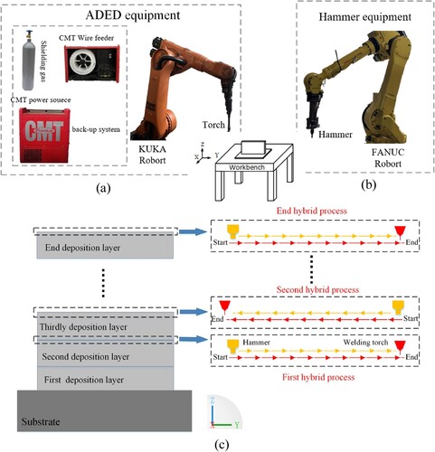
The in-situ hammering is performed on the ADED wall when the ADED process is completed and cooled to 25 °C. The direction of hammering is aligned with the deposition direction of the same layer. The inter-layer hammering is introduced after the deposition of layer 2 because the deposition of layer 1 reinforces the junction position between the substrate and the ADED wall. The hammer motion is shown by the yellow path in Figure 2c. The distance between the hammer and the deposited layer is adjusted to 10 mm. Each layer is then hammered once using a mechanical arm equipped with a pneumatic hammer with a 12 mm radius. The hammering frequency is set at 7 Hz. The deposition of the next layer begins directly after the ADED wall has cooled to 25 °C. Each new deposition layer is hammered once and then the next layer is deposited and hammered. On the other hand, the specimen prepared by ADED alone (group 2) uses the same deposition parameters as group 1.

2.3. Construction of inter-layer hammering hybrid ADED finite element model

2.3.1. Construction of ADED finite element model

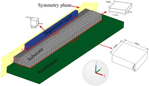
The finite element model of ADED (Deposition model) is constructed using the DED (Directed Energy Deposition) function in Simufact welding® software. The thermodynamic behaviour of the ADED process can be calculated by direct coupling and indirect coupling methods. In this study, the temperature field, stress, and strain field in the ADED process are calculated based on the direct coupling method of the Marc solver. Figure 3 provides a constitution of the deposition model, which consists of a worktable (rigid body), substrate (100mm×60mm×5 mm), and deposition layers (70mm×5mm×2.5 mm). It should be noted that only the model of the first layer deposition is shown in Figure 3. Only half of the deposition model is created because of the symmetric nature of the thermal and force boundary conditions along the deposition direction. Symmetric constraint boundary conditions are applied to the Y-Z cross-section. The workbench is considered completely fixed during the deposition process. The relationship between the substrate and the workbench was defined as bonding since the substrate was small in the experiment. Gornyakov et al. [15] discussed the feasibility of this approach, it is concluded that this simplification will not affect the prediction of the finite element model on stress variation trend. The graded mesh method [2] is employed for meshing the substrate to balance accuracy and computation time. Small meshes with dimensions of 0.5 mm×0.5 mm×0.5 mm are used for modelling the deposition layer and its vicinity. The mesh size increases to 3 mm×2.5 mm×1 mm at the edges of the substrate. The meshes number of the substrate is 9520, while each deposition layer comprises 3600 meshes.

Figure 3. Composition of the deposition finite element model.

The Goldak-double ellipsoidal heat source model [23] is used to simulate the heat input, and its heat flux distributions are described by Formulas (2) and (3). Where $q_1$ and $q_2$ describe the power density ($\mathrm{W}/{\mathrm{m}}^3$) distributions in the anterior and posterior hemispheres respectively. P is the energy input (W), and the values are given in Table 2. $\eta$ is the efficiency of the heat source. Figure 4 provides the size parameters of the heat source, and the numerical values of these parameters are shown in Table 2. The energy density used in the deposition of the first layer is greater than that of the subsequent because the deposition strategy of the ‘high current + linear path’ approach was adopted in the first layer deposition in the experiment. The ‘element birth’ technique [24] is implemented during the ADED process. The convection and radiation coefficients are assumed to be temperature-independent with values of 30 $W/m^2\ast K$ and 0.6, respectively. Considering the enhanced cooling effect of the platform on the substrate, the heat convection coefficient on the substrate bottom surface was set to 237$W/m^2\ast K$ [24]. The initial temperature of the deposition model is set at 25°C, and the environment temperature is also set to 25°C. The cooling time after the end of deposition is set to 300 s. However, once the temperature of the deposition layer reaches 25°C, the deposition process ends, and the hammering of the newly deposited layer begins. (2) $q_1={\displaystyle \frac{6\sqrt{3}{f}_1\mathrm{P\eta }}{\pi a_1\mathrm{bc}\sqrt{\pi }}\exp \left(-3{\displaystyle \frac{x^2}{a_1^2}}\right)\exp \left(-3{\displaystyle \frac{y^2}{b_{}^2}}\right)\exp \left(-3{\displaystyle \frac{z^2}{c_{}^2}}\right)}$(2) (3) $q_2={\displaystyle \frac{6\sqrt{3}{f}_2\mathrm{P\eta }}{\pi a_2\mathrm{bc}\sqrt{\pi }}\exp \left(-3{\displaystyle \frac{x^2}{a_2^2}}\right)\exp \left(-3{\displaystyle \frac{y^2}{b_{}^2}}\right)\exp \left(-3{\displaystyle \frac{z^2}{c_{}^2}}\right)}$(3)

Figure 4. Model of double ellipsoidal heat source.

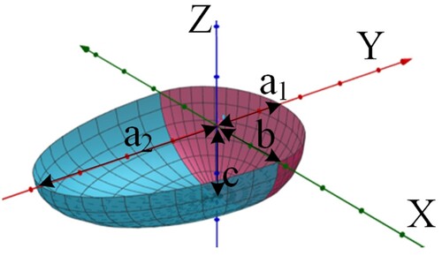
Table 2. Parameters of double ellipsoidal heat source model.

Layer	Heat source parameters (mm)				Travel speed$\mathrm{mm}/\mathrm{s}$	Energy density$\mathrm{J}/\mathrm{mm}$	Efficiency	P (W)
	$a_1$	$b$	$a_2$	$c$
1	2.5	3	6	2.7	10	196	0.7	2800
2—8	3	3.4	6	3	5	168	0.7	1200

2.3.2. Construction of the hammering finite element model

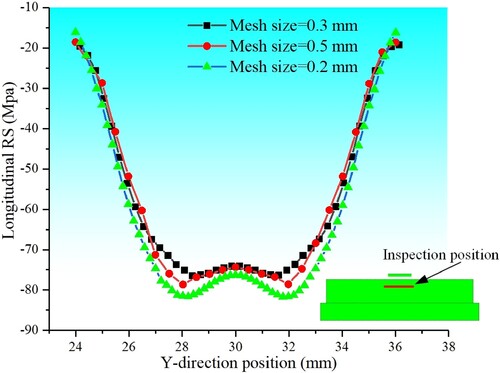
The hammering finite element model (Hammering model) was constructed in Simufact Forming® (Figure 5). The hammering model inherits the calculation results (Including stress, strain, warping, and temperature field) and mesh of the deposition model. A rigid cylinder with a radius of 12 mm is used to simulate the hammer. The hammering model adopts the same force boundary conditions as the deposition model. The initial temperature of both the substrate and the ADED wall is 25°C. The hammer and the ADED wall do not slide relative during the hammering process. The friction between the hammer and the deposition layer was set to 0.2 referring to the friction coefficient of structural steel. Figure 6 shows the mesh independence verification results of the hammering model. A series of inspection points located in the Z-Y plane of the hammering model, 2 mm from the top of the ADED wall, were selected to extract the longitudinal RS. The longitudinal RS results of the smaller mesh size (0.3, 0.2 mm) were compared with the hammering model mesh (0.5 mm). A series of inspection points 5 mm from the top of the ADED wall directly below the hammer were set up to capture the changes in the stress distribution of the ADED wall during the hammering process. As can be seen from Figure 6, as the mesh size decreases, the position of the inspection points with the largest change in longitudinal RS changes by 3.8% (the size mesh changed from 0.5 mm to 0.2 mm). And the calculation time has increased by four times. Considering the calculation accuracy and calculation cost, a 0.5 mm mesh size can be recognised as suitable for the hammering model.

Figure 5. Composition of the hammering finite element model.

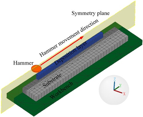
Figure 6. Hammering model mesh accuracy verification.

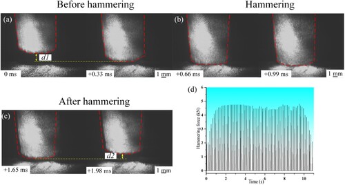
Hammering depth ‘a’ as shown in Figure 7a is used to simulate the hammering effect on the wall. Figure 8 shows the measuring method of the hammering depth. A full hammering process was filmed using a high-speed camera. The value difference of 0.4 mm between point ‘d’ and point ‘e’ at the top of the deposition layer is taken as the hammering depth. To avoid the hammering depth measurement error caused by the uneven surface of the deposition layer, six evenly distributed measuring points were set on the deposition layer to measure the hammering depth ‘$a_i$’. Bring the measured value ‘$a_i$’ into formula (4) to calculate the hammering depth ‘a’. The ‘h’ was the distance between the top of the ADED wall and the hammer, and its value was set to 10 mm in the hammering model. The hammer motion can be decomposed into a ‘reciprocating cycle motion’ (as shown in Figure 7c) and a ‘step motion’ (as shown in Figure 7d), which together complete the hammering process. The frequency setting reference experiment of ‘reciprocating motion’ is 7 Hz. The starting position of the hammer is the origin and then moves 10.4 mm in the negative direction of Z which includes the distance between the hammer and the top of the ADED wall (‘h’) and the hammering depth (‘a’). (4) $a=\sum _{i=1}^n{\displaystyle \frac{a_i}{n}}$(4) To verify the accuracy of simulating the hammering effect through the hammering depth, the hammering process was captured using a high-speed camera with a frame number ‘f’ of 3000 and the hammering force was calculated based on the photos taken. Hammering force is calculated by the impulse theorem and the momentum theorem. Taking the hammer as the research object, the impulse ($I=F\ast t$) generated by the force of the ADED wall on the hammer during a full hammering results in a change in hammer momentum ($\mathrm{\Delta }P=m\ast \mathrm{\Delta v}$) before and after hammering. The contact time (‘t’) of the hammer with the ADED wall can be obtained from Figure 9b. It can be seen from Figure 9b that the contact time ‘t’ between the hammer head and the deposition wall during the hammering process is 1/f. The change in the speed of the hammer before ($v_0$) and after ($v_1$) hammering can be calculated through the Figure 9a and c, respectively. As shown in Figure 9a and c, the displacement difference ‘d1’ with 0.0027 m and ‘d2’ with 0.002 m is calculated by the position of the hammerhead recorded in two consecutive frames of photos. The velocity of the hammer before ($v_0$) and after ($v_1$) hammering can be calculated by ‘$v=\mathrm{df}$’. It should be noted that the closer the measurement time of the hammer displacement during the rebound process aligns with the completion time hammering, the more effectively it mitigates the hammer spring on the velocity of rebounding. The weight of the hammer ‘m’ in the experiment is 0.1 kg. The weight of the hammer and the velocity of the hammer before ($v_0$) and after ($v_1$) the hammer is brought into formula 5 to calculate the variable of hammer momentum before and after the hammering. And then obtain the impulse (‘I’) of the ADED wall against the hammer. Finally, brought the I into formula (6) to calculate the hammer force of 4.23kN. Figure 9d shows the hammering force exerted by the hammer on the deposition wall in the hammering model, and the average value of the hammering force is 4.5 kN. The hammering force produced by displacement control in the simulation is slightly greater than that measured in the experiment. The error between the hammering force extracted by the hammering model and measured in the experiment is 6.3% (Compared with the hammer force measured in the experiment), which is acceptable. (5) $I=\mathrm{\Delta P}=m\ast \mathrm{\Delta v}=m\ast (v_0-v_1)$(5) (6) $I=F\ast t$(6)

Figure 7. Decomposition of hammer motion during hammering process, (a) Hammering operation schematic diagram, (b): Hammering motion law in the Y direction (local), (c): Hammering motion law in the Z direction (local).

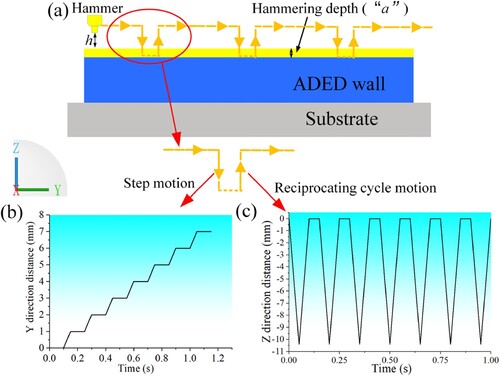
Figure 8. Measurement of the hammering depth value, (a) Before hammering, (b)Hammering, (c)After hammering.

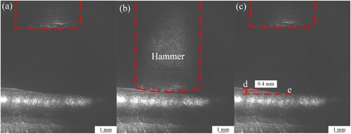
Figure 9. High-speed camera images of the hammering process, (a) The position of the hammer captured by the high-speed camera before the hammering, (b) The contact time between the hammer and deposited wall captured by the high-speed camera, (c) The position of the hammer captured by the high-speed camera after the hammering, (d) The hammering force extracted from the hammering model

2.3.3. Construction of ADED hybrid hammering finite element model

The key to constructing the ADED hybrid inter-layer hammering finite element model (Hybrid model) can be summarised in two main aspects. Firstly, it is essential to determine how to transfer the field distribution data, including stress, strain, deformation, and temperature fields, calculated by the deposition model (or hammering model), to the hammering model (or deposition model) as the initial state. This ensures a consistent starting point for the subsequent analysis. Secondly, it is critical to consider the effect of hammering on the deposition layer mesh deformation. This deformation is reflected in the region of the deposition layer that is hammered becomes undulating and the position of the mesh node changes. There is a need that requires a strategy for constructing subsequent deposition layers based on deformed mesh. Since the deposition wall mesh is cycled between the deposition and hammering models, only the correspondence between the newly added deposition layer and the mesh nodes of the deposition wall top is considered.

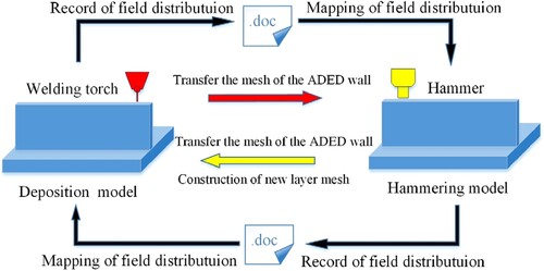
The ‘field circulation transfer’ technology was proposed to solve the transfer of field distribution between models. As shown in Figure 10, this technology uses a specialised file to record the field distribution data calculated by the deposition model. When the deposition process is complete, the mesh of the deposition wall is first imported into the hammering model through the software interface. Next, the field distribution data recorded in the file is read and mapped onto the deposition wall mesh in a node-to-node way. The field distribution data calculated by the deposition model is regarded as the initial state of the hammering model by the ‘field circulation transfer’ technology. The ‘field circulation transfer’ technique allows for the bi-directional transfer of field distributions between the deposition model and the hammering model.

Figure 10. ‘Result cyclic transfer’ technology schematic diagram.

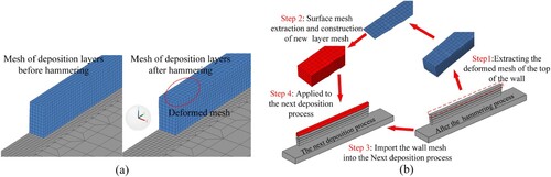
The hammering results in changes in the position of the top deposition layer mesh nodes (shown in Figure 11a deformed mesh), and these changes are difficult to predict. Therefore, when a new layer is to be deposited, it is necessary to consider the correspondence between the newly added layer and the mesh of the original deposition wall top. The ‘surface mesh extraction and reconstruction’ technique is proposed to solve the problem of constructing a new layer mesh. The ‘surface’ here refers to the deformed mesh at the top of the deposition wall. Figure 11b shows the details of ‘surface mesh extraction and reconstruction’. Step 1, the top of the deposition wall mesh is extracted and imported into Simufact mesh® after the hammering process. It should be noted that the ‘extraction’ can be understood as ‘duplication’, and not change the deposition wall mesh. In step 2, only the surface mesh is retained to construct the new layer mesh. Steps 3 and 4, the new layer mesh and the deposition wall mesh are imported into the next deposition process and used for subsequent simulations.

Figure 11. ‘Surface mesh extraction and reconstruction’ technology, (a) Deformed mesh of deposition layer after hammering, (b) ‘Surface mesh extraction and reconstruction’ technology schematic diagram.

Figure 12 shows the application details of the ‘field circulation transfer’ technology and ‘surface mesh extraction and reconstruction’ technology in the hybrid model. The ‘field circulation transfer’ technique is used to transfer the field distribution data calculated by the deposition model to the hammering model when the deposition process is completed. Similarly, when the hammering process is completed and a new deposition process, not only the field distribution data and deposition wall mesh are transferred, but also the new layer mesh based on ‘surface mesh extraction and reconstruction’ technology is added for a new round of deposition simulation.

Figure 12. Working flow chart of the hybrid finite element model.

2.4. Setting of the experiments and finite element models

Table 3 presents the experimental setups in this study, the experiment was divided into two categories: group 1 was the preparation of the ADED wall with inter-layer hammering, and group 2 was the ADED alone. Two groups’ experiments are used to verify the results of predictions. In addition, three groups of simulation models were set. Model 1 simulated the hybrid process of eight inter-layer hammering and ADED, with a focus on investigating the stress evolution during the hybrid process. Model 2 simulated the deposition of the ADED wall with the same number of layers as model 1. It is used to compare the prediction result with Model 1 and obtain the effect of hammering on reducing stress. Model 3 was designed to simulate a single inter-layer hammering without considering the ADED process. Its purpose was to capture the impact of hammering more clearly on wall strain and stress.

Table 3. Setting of the experiments and finite element models.

Type		Conditions	Purpose
experiment	Group 1	ADED hybrid inter-layer hammering	Used to verify finite element models
	Group 2	ADED alone
Simulation	Model 1	ADED hybrid inter-layer hammering	Study the evolution of RS and deformation under the interaction of hammering and deposition
	Model 2	ADED alone	The control group of model 1.
	Model 3	A single inter-layer hammering process without the ADED	Studying the distribution characteristics of a single hammering- introduced longitudinal deformation and stress.

2.5. Model computation

The models in this study were calculated on a computer with 8 cores, specifically a 13th Gen Intel® Core™ i5-13400F. The calculation method utilised for the deposition and hammering model is Simufact’s Paradiso calculation method, which is a robust direct solver suitable for small, medium, and large-sized models. This solver can handle all element types and is advantageous for unstable processes. The element type employed in both the deposition and hammering models is Tet134, which is a type of element with two degrees of freedom for temperature and displacement. Given the particularity of the deposition hybrid hammering finite element model, it is necessary to model the newly deposited layer in real time. Consequently, the number of meshes and the computation time for each process increase. The calculation of the last deposition model, which consists of 38,320 elements, took approximately 30 min. Subsequently, the inter-layer hammering process model took around 4 h to compute. It is worth noting that these calculation times may vary depending on the specific hardware configuration and computational resources available.

3. Results

3.1. Verification of the finite model

To validate the hybrid model, a comparison was made between the predicted results and experimental data for several parameters, including the ADED wall cross-section morphology (Built by inter-layer hammering hybrid ADED and ADED alone), heat input, warping, and RS.

3.1.1. Comparison of cross-section morphology

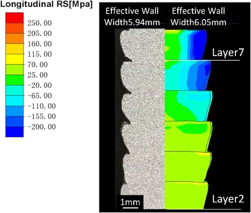
Figure 13 shows the cross-section morphology of the ADED wall of experiment 1 and model 1. Model 1 successfully predicted the width and height layers of the hammered wall, which matched the results from experiment 1. There is a slight discrepancy observed in the width, with the predicted width (6.05 mm) differing from the measured width (5.94 mm) by 0.1 mm. The predictions for the average height of the hammered wall align well with the experimental measurements. Model 1 predicted a height of 14.48 mm, while the measured height was 14.72 mm.

Figure 13. Comparison of the ADED wall cross-section morphology between experiment 1 and model 1 predicted.

3.1.2. Verification of heat input

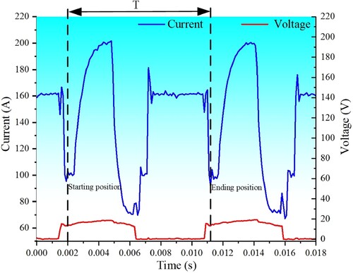
The research on heat input is divided into three parts: heat input verification, heat source size verification, and temperature history verification. Figure 14 shows the CMT current and voltage characteristic curves during deposition. The heat source power used in the deposition model is a constant value of 1200 W. The measurement frequency of the CMT characteristic curve is 10 kHz. The measured current and voltage in one period are brought into formula (7) to calculate the average power value in one CMT period as 1267.51W. The error between the heat source power used in the deposition model and the measured value is 5%. The heat input set in the deposition model is in good agreement with the experiment. (7) $P_{\mathrm{average}}=\sum _{i=1}^n{U}_i\ast I_i/n$(7)

Figure 14. Current and voltage characteristic curve of Cold metal transition (CMT).

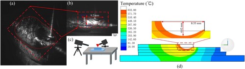
Figure 15 shows a comparison of the size of the molten pool captured by the high-speed camera and the size of the heat source in the deposition model. The frame number used for shooting was 2000. The welding wire used in the deposition process was 1.2 mm, and the maximum size of the molten pool in the experiment was calculated by referring to the diameter of the welding wire as 9.2 and 4.3 mm. The maximum size of the molten pool measured in the deposition model is 8.55 and 3.66 mm. The margin of error was 7% and 14%, respectively.

Figure 15. Verification of molten pool morphology (a) (b) Molten pool morphology captured by high-speed camera, (c) Shooting Angle, (d) size of heat source in deposition model.

Figure 16 shows a comparison of temperature history between the experiment and deposition model inspection points. The temperature history of inspection points in model 1 is obtained by pre-labeling corresponding cell nodes, and the temperature history of the inspection point in the experiment was obtained by using a type K thermocouple. Table 4 provides the coordinates of the inspection points used for the temperature history measurements. Figure 17 shows the position of the inspection point on the substrate. Take the L1P1 for example, which indicates that the temperature at point P1 was measured during the deposition of the first deposition layer. It can be found that the maximum temperature and history of temperature change of each inspection point in model 1 and experiment 1 are in good agreement. This indicates that the heat input utilised in the model was appropriate.

Figure 16. Position of thermal history inspection points.

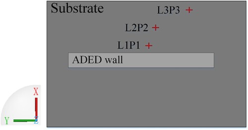
Figure 17. Comparison of inspection points thermal history between experiment and finite element models. (a) Temperature history at the L1P1 inspection point, (b) Temperature history at the L2P2 inspection point, (c) Temperature history at the L3P3 inspection point.

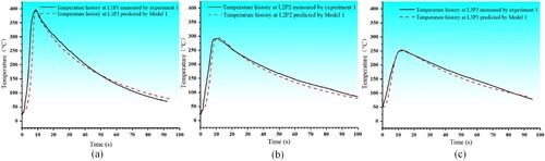
Table 4. Location of temperature inspection point (mm).

	X	Y	Z
L1P1	4.5	52.5	5.0
L2P2	7.5	51.0	5.0
L3P3	12.5	45.0	5.0

3.1.3. Verification of RS results

XRD method has been widely used to measure the RS of parts [25–28] and is a common and reliable method. Zhang et al. [29] simulated the RS of Ti-6Al-4V square plates prepared by six different scanning strategies and measured RS by XRD. The predicted results are in good agreement with the measured values. Najib et al. [30] used XRD to measure the RS at the weld position in friction stir welding and compared the results with those measured by the contour method, and the results showed consistency. Three-dimensional stress was measured using the XRD method after removing the clamps. The XRD measurement parameters are given in Table 5. The distribution of inspection points is shown in Figure 18b. The ADED wall was processed as shown in Figure 18a. Initially, the wire-cutting technique was employed to remove the mechanical removal region. Subsequently, the electrolytic method was used to eliminate the electrolytic removal region, ensuring the elimination of any additional mechanical stress.

Figure 18. The verification diagram of RS. (a): Pre-processing of the specimen before inspection, (b): Inspection point of RS.

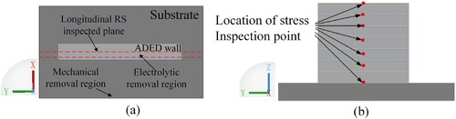
Table 5. X-ray diffraction scanning parameters.

Measuring method	side-incline method	Crystal orientation	{222}
Anode Material	CrK$\alpha$	Scanning current	25mA
Wavelength	1.790nm	Scanning voltage	30KV

The method of XRD-$\mathrm{si}{\mathrm{n}}^2\psi$ was used to analyse the measurement results of XRD, and calculated stress in the three directions of the inspection point. The measurement of lattice plane spacing D$\psi$ was carried out on an XRD diffractometer produced by Proto, Canada. The parameters of XRD diffraction used in the measurement process are shown in Table 5. The principle of XRD stress measurement tries to consider the lattice strain caused by a certain stress state as consistent with the macroscopic strain obtained by the elastic theory. The lattice strain can be measured by XRD through the Bragg equation so that the macroscopic stress can be calculated from the measured lattice strain. In the detection plane with a $\phi$ angle, the normal direction of a crystal plane satisfying the Bragg equation (hkl) is $\psi$ angled to the normal direction of the material surface, and the main formula of XRD-stress measurement can be written as (4) [31]. Among them, ‘E’ and ‘$\mu$’ are Young's modulus and Poisson's ratio of the material, respectively. The crystal plane spacing of the material in the non-stress state is $D_0$, and the crystal plane spacing is D$\psi$ under the action of stress ${\sigma }_{\phi }$. Where $(\mu /E)({\sigma }_1+{\sigma }_2)$ is a constant term. The figure ${\epsilon }_{\phi ,\psi }-\mathrm{si}{\mathrm{n}}^2(\mathrm{\Psi })$ is drawn with The measured lattice strain at the corresponding angle $\psi$, and the slope $(1+\mu /E){\sigma }_{\phi }$ is obtained by using the least square method. Then the stress component ${\sigma }_{\phi }$ acting on the measured cross-section with a normal angle of $\phi$ can be obtained. (8) ${\epsilon }_{\phi ,\psi }={\displaystyle \frac{D_{\psi }-D_0}{D_0}=\left({\displaystyle \frac{1+\mu }{E}}\right){\sigma }_{\phi }\mathrm{si}{\mathrm{n}}^2(\psi )-\left({\displaystyle \frac{\mu }{E}}\right)({\sigma }_1+{\sigma }_2)}$(8)

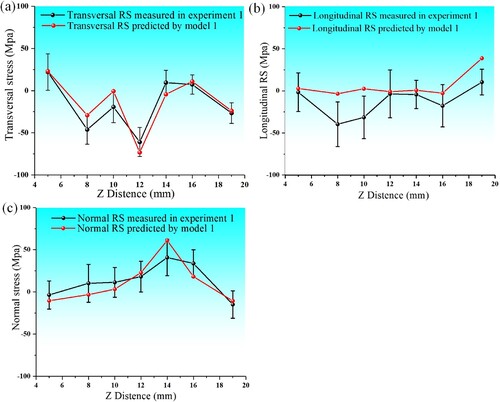
Three-dimensional RS is depicted at various distances from the underside of the substrate (5, 8, 10, 12, 14, 16, and 19 mm) in Figure 19. According to the characteristics of XRD RS measurement, the measured value can be considered as an average value of the RS in the 1 mm range of the each RS inspection point. This distribution of stress measurement points is representative considering the height of the ADED wall (19.48 mm). Model 1 predicts the longitudinal RS distribution, as shown in Figure 19b, is in good agreement with the results of experiment 1 in general. The maximum discrepancy with a value of 20 MPa between the predictions and measurements is observed at 8 and 10 mm. The bonding relationship between the substrate and the workbench in the hybrid model may cause the stress of the wall near the substrate to be greater than the measured value [15]. Additionally, the experimental measurements for transverse (Figure 19a) and normal (Figure 19c) stress range from −70 MPa to −25 MPa and −20 MPa to −30 MPa, respectively. The RS values predicted by the model at these seven positions all fall within the range allowed by the experimental measurements, and the tendency of the predicted value agrees with the measured value. The comparison of stress results demonstrates the model’s ability to accurately predict RS within the acceptable range observed in the experiment.

Figure 19. The RS of experiment 1 and model 1 after removing the clamps. (a) Longitudinal (Y direction) RS, (b) Transversal (X direction) RS, (c) Normal (Z direction) RS.

3.1.4. Comparison of ADED wall warping

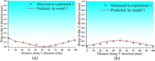
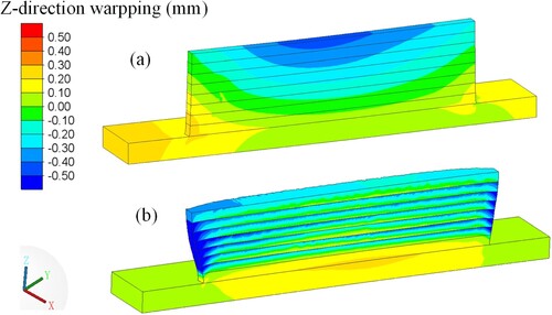
The substrate warping of experiments 1 and 2 after removing the clamps was measured using a 3D scanner and compared with the results predicted by models 1 and 2. To ensure stability during measurements, the ADED wall was placed on a measurement table and supported as shown in Figure 20. The scanner’s laser was used to collect the contour of the deformed substrate, which was then extracted and used to compare with the predicted results. The comparison aimed to assess the inhibitory effect of hammering on warping. Figure 21 shows the bending warping along the bottom of the substrate after removing the clamps. Figure 21a compares the Z-direction warping of the substrate between model 2 and experiment 2, while the warping comparison between model 1 and experiment 1 is shown in Figure 21b. In Figure 21a, it can be observed that there is a slight upward bending of the substrate after removing the constraints. Model 2 predicts a maximum warping of 0.196 mm, while the warping measured in experiment 2 is 0.20 mm. Moreover, the trend of warping predicted by the model is in good agreement with the experimental trend. For the warping of the hammered wall shown in Figure 21b, model 1 predicts an upward warping magnitude of 0.13 mm, whereas the experiment reveals an upward warping of 0.12 mm.

Figure 20. The scanning way of the ADED wall warping.

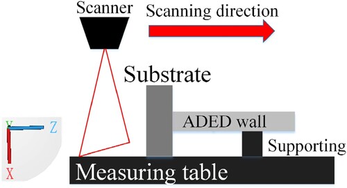
Figure 21. Comparison of the substrate warping of the experiment with the model prediction, (a) ADED alone, (b) ADED hybrid inter-layer hammering.

3.2. Formation of stress and plastic strain during a single inter-layer hammering process

3.2.1. Longitudinal plastic strain and stress

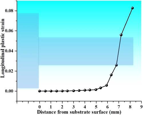
Inter-layer hammering can be regarded as a hybrid process involving multi-rounds of ADED and post-deposition hammering. To capture the impact of hammering more clearly on wall strain and stress, a single inter-layer hammering was simulated without considering the effect of the ADED process (model 3). Figure 22 shows the distributions of the longitudinal plastic strain predicted by model 3. Hammering introduces the tensile plastic strain in the wall, both accompanying transverse and longitudinal plastic strains. The longitudinal plastic strain and stress are focused on because of the significant longitudinal shrinkage that occurred during the process of ADED [7]. As shown in Figure 22a, the wall in front of the hammer produces a longitudinal tensile plastic strain region. As the hammering process continues, Longitudinal tensile plastic strain induced by hammering gradually extends along the direction of hammer movement and eventually occupies the top of the wall and a certain depth (Figure 22 b, c). Figure 23 shows the distribution of the longitudinal plastic strain of the ADED wall along the building direction. A large longitudinal plastic strain with 0.08 is generated at the top of the wall. A gradual reduction of the longitudinal tensile strain in the building's negative direction due to constrained by the material at a deeper position. The longitudinal strain level is almost 0 at the position of transition between the substrate and deposition wall. The longitudinal tensile plastic strain region extended up to 8 mm from the top of the wall. Two large longitudinal plastic strain regions were generated due to the absence of constraints at both ends of the wall.

Figure 22. The longitudinal plastic strain formation during a single inter-layer hammering process (a) The beginning of the hammering movement. (b) The middle stage of the hammering movement. (c) The final state of the ADED wall after the hammering.

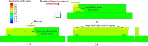
Figure 23. Longitudinal plastic strain in the walls introduced by a single inter-layer hammering.

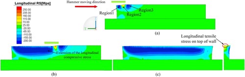
Figure 24 shows the longitudinal RS distribution under the condition of longitudinal plastic strain distribution shown in Figure 22. Three regions were defined to describe the longitudinal stress evolution at the beginning of the hammering (Figure 24 a) according to the level of longitudinal stress. Region 1 is located below the contact surface between the hammer and wall, while regions 2 and 3 are in front of the hammer below the wall surface. The tensile plastic strain introduced by hammering resulted in longitudinal compressive stress in regions 1 and 3, while region 2 was the longitudinal tensile stress. Region 2 was always generated in front of the hammering position and moved forward with the hammer during the process of hammering. As the hammering persisted, the compressive stress in region 3 underwent a transient conversion to tensile stress before subsequently transitioning back into compressive stress, amalgamating with the tensile stress in region 2 and contributing to the extension of longitudinal compressive stress. The longitudinal compressive stress occupied the core of the wall after the hammering process. The tensile stress with 102 Mpa was generated at the wall top (Figure 24c). Along the negative direction of the building, the tensile stress rapidly transforms into compressive stress and reaches its maximum value of −30 Mpa at 3 mm from the top of the wall. Subsequently, it gradually decreases to zero. It is worth noting that the longitudinal tensile plastic strain introduced by the hammering at the top of the wall is much greater than the core of the wall, but the top of the wall produces a large longitudinal tensile stress. This is contrary to the longitudinal compressive stress in the core region of the wall.

Figure 24. The longitudinal stress evolution during a single inter-layer hammering process. (a) The beginning of the hammering movement. (b) The middle stage of the hammering movement. (c) The final state of the ADED wall after the hammering.

3.2.2. The discrepancy of effects of inter-layer hammering on ADED wall top and core

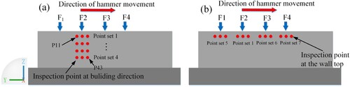
The discrepancy in longitudinal plastic stress introduced by hammering at the top and core of the wall is an interesting phenomenon. As shown in Figure 25a, to investigate the discrepancy between the effect of hammering on the top and core of the wall, a series of inspection points are placed along the building direction. These inspection points are located at different distances from the top of the wall, specifically at intervals of 0.5, 1.5, 2.5, and 3.5 mm, while the distance between the inspection points sets is 5 mm in Figure 25b. The inspection points along the wall were labelled using the matrix method, where each point is assigned a label such as Pmn. Here, m represents the row number (m = 1, 2, 3, 4) and n represents the column number (n = 1, 2, 3). For example, P11 denotes the initial point located at the top left corner of the wall, while P43 represents the final point situated at the bottom right corner of the wall. The F1-4 represents several adjacent hammerings during a single inter-layer hammering process. The inspection points were positioned beneath the contact surface between the hammering of F2 and the wall. More specifically, Pm2 was directly below the contact surface, Pm1 was to the left of Pm2 in terms of the hammering direction, and Pm3 was positioned to the right of Pm2.

Figure 25. Setting of inspection points at building direction and wall top, (a) inspection points at building direction, (b) inspection points at wall top.

Figure 26a shows the evolution of the longitudinal plastic strain of the wall top material (set 1) with the calculation step. The F1, F2, and F3 marked on the curve in Figure 26 represents the action time of hammering. It can be seen from Figure 26a that hammering induces compressive plastic strain at P13 and P11, resulting in the compression of the material at P13 and P11 towards the hammering centre (P12). Hammering-introduced tensile plastic strain at P12 leads to a stretching tendency of the material at P12. Withers et al. [29] proposed that the RS is caused by the‘misfit’ between regions caused by the deformation of the material. The stretching tendency at P12 and the compression at P13 and P11 exacerbate the ‘misfit’ between the regions represented by set 1's different inspection points. Figure 27b shows the plastic strain at the core of the wall. A stretching tendency at P23 and P22 because hammering-introduced tensile plastic strain at P23 and P22. It does not exacerbate the degree of ‘misfit’ between the regions because the direction of the expansion trend is the same. However, the Hammering-introduced compressive plastic strain at P21 will lead to the ‘misfit’ between the regions represented by P21 and P22. The degree of ‘misfit’ between the regions will decrease with the increase of the distance from the wall top. A similar strain evolution as observed in set 2 takes place (Figure 27 c, d) in the deeper region of the ADED wall. The difference in plastic strain results in a difference in the degree of ‘misfit’ between the top and core of the wall. This difference may be the cause of tensile stress at the top of the wall and the longitudinal compression stress distribution on the wall described in section 3.2.1.

Figure 26. Longitudinal plastic strain evolution of building direction inspection points with the calculation step. (a): Longitudinal plastic strain of set 1, (b): Longitudinal plastic strain of set 2, (c): Longitudinal plastic strain of set 3, (d): Longitudinal plastic strain of set 4.

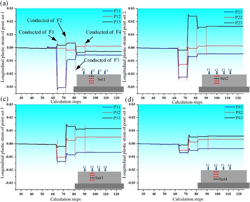
Figure 27. Longitudinal plastic strain evolution of the wall top inspection points with the calculation step. (a) Longitudinal plastic strain of set 5, (b) Longitudinal plastic strain of set 1, (c) Longitudinal plastic strain of set 6, (d) Longitudinal plastic strain of set 7.

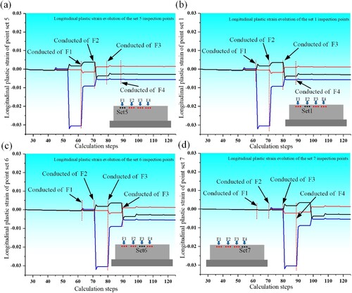
To eliminate the contingency of the top-of-wall strain evolution in Figure 26 a, a series of inspection points (Figure 25 b) was set at the top of the wall along the direction of the hammer movement, and the results of the longitudinal plastic strain during the hammering were extracted. As shown in Figure 27. the values and trends of longitudinal plastic strain at inspection points in different regions on the wall top were the same.

3.3. Stress during the hybrid process

3.3.1. Characteristics of the longitudinal stress distribution in the ADED wall

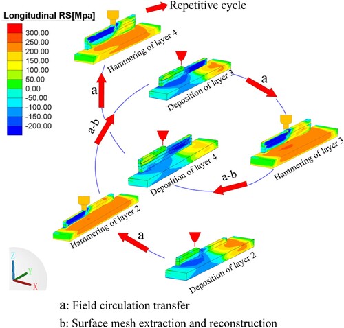
Figure 28 shows the distribution of longitudinal stress in the ADED wall predicted by model 1. The Z-X inspection plane for the longitudinal stress is positioned at the midpoint of the Y-axis (Figure 28e). As shown in Figure 28a, the tensile RS with an average value of 220 MPa was generated in the wall after the deposition of layer 2. The highest tensile longitudinal RS with 230 MPa was observed near the transition between the substrate and the wall. The longitudinal tensile stress of the ADED wall is reduced by the subsequent hammering of layer 2 and transforms into compressive stress. Two regions can be identified according to the stress distribution characteristics after the hammering of layer 2 (The right side of Figure 28a.). The outer region of the wall, referred to as region 1, with a width that accounts for one-third of the wall’s total width and extends to a depth of 4 mm in the Z direction. Region 1 is more prone to deformation under the action of hammering due to the lack of lateral constraints (X direction), resulting in large longitudinal compressive RS. Region 2, located at the core of the ADED wall, is constrained by lateral constraints of region 1 during the hammering process. The depth of influence of region 2 is greater than that of region 1 although the mitigation effect on stress is not as good as that of region 1. As shown in Figure 28b, the tensile RS with 201 Mpa was regenerated in the wall affected by the deposition of layer 3. The subsequent hammering of layer 3 has a similar mitigating effect on the longitudinal RS as the hammering of layer 2. Two regions with different stress mitigation effects can still be observed on the section of the wall, but the range is increased compared to Figure 28a (right).

Figure 28. Cloud diagram of longitudinal RS of the ADED wall cross-section, (a) (b) (c): the hybrid process of layers 2, 3, and 7 (the left is the longitudinal stress result after ADED and the right cloud diagram is after hammering), (d) ADED wall only deposition, (e) The position of the inspection plane.

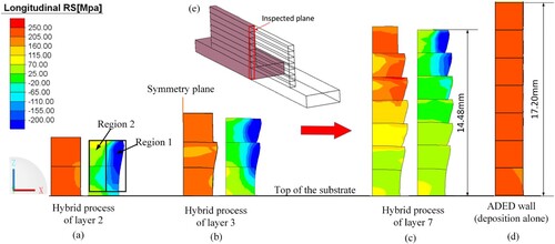
Comparing the stress level distribution in the wall section after the deposition of layers 2 and 3, it can be observed that although the tensile stress generated by the deposition of layer 2 is reduced by the hammering of layer 2 (Figure 28a, right), the longitudinal tensile stress on the wall is not significantly reduced after the deposition of layer 3 (Figure 28b, left). This indicates that affected by the deposition of layer 3, the mitigation effect of the hammering of layer 2 on the longitudinal tensile RS was not retained. However, following the deposition of layer 7 (Figure 28c), a notable decrease in the longitudinal RS was observed in the second deposit layer compared to Figure 28(a, b). This indicates that the mitigation effect of inter-layer hammering on the longitudinal stress was retained through subsequent rounds of hybrid process, i.e. the mitigation effect of multi-round inter-layer hammering on the stress of layer 2 resulted in a significant decrease in the longitudinal tensile stress of layer 2. In terms of height, the wall after the hammering of layer 7 was reduced in height by 2.72 mm. The average hammering depth per layer was 0.39 mm, slightly less than the predetermined hammering depth of 0.4 mm.

3.3.2. Longitudinal stress distribution in the ADED wall

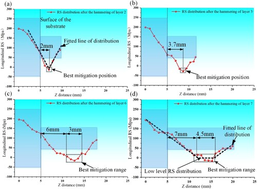
The longitudinal RS distribution in the wall after the hybrid process of layers 2, 3, 6, and 7 for model 1 was extracted to better demonstrate the dynamic effects of inter-layer hammering on RS during the hybrid process. The inspection plane was positioned as shown in Figure 28(e). A new concept of ‘best mitigation position’ where the position with the most significant stress reduction is proposed to reflect the dynamic change of stress distribution in the wall during the hybrid process.

Figure 29a shows the stress distribution after the hammering of layer 2. The stress at the transition position between the substrate and the wall and the top of the wall is 75 and 82 Mpa, respectively. The position of the ‘best mitigation position’ was observed 2 mm from the substrate surface, with a longitudinal stress level of −25 MPa. Overall, a V-shaped trend stress distribution on the wall was observed along the building direction (Figure 29a, the black fitted line). The ‘best mitigation position’ with an average value of −25 Mpa is changed from 2 mm away from the substrate surface to 3.7 mm after the hammering of layer 3 (Figure 29b). In addition, the stress at the transition position between the substrate and the wall, and the top of the wall reduce to 56 and 52 Mpa, respectively. After the hammering of layer 6 (Figure 29 c), The ‘best mitigation position’ with an average value of −10 Mpa is observed within the range of 6-9 mm from the substrate surface. Compared with the stress distribution after the hammering of layer 2, the ‘best mitigation position’ changed from a point position to a range after the hammering of layer 6, and the distance from the substrate surface changed from 2 mm to 6 mm. The stress at the transition position between the substrate and the wall and the top of the wall increased to 126 and 82 Mpa, respectively. The change of the ‘best mitigation position’ is more pronounced in the hammering of layer 7. The ‘best mitigation position’ changed from 6-9 mm away from the substrate’s surface to a new range of 7-11.5 mm after the hammering of layer 7 (Figure 29d). There are two significant differences between the stress distribution fitting line of the hammering of layers 2 and 7, which are reflected in the increase in the distance from the substrate surface and the range of the ‘best mitigation position’.

Figure 29. The accumulation of mitigation effect of hammering on longitudinal tensile stress in the hybrid process: (a) Longitudinal stress distribution after the hammering of layer 2, (b) Longitudinal stress distribution after the hammering of layer 3, (c) Longitudinal stress distribution after the hammering of layer 6, (d) Longitudinal stress distribution after the hammering of layer 7.

3.3.3. Longitudinal stress at the local position in the ADED wall

During the hybrid process, it is common and normal that the mitigation effect of the hammering on RS is eliminated by the subsequent deposition process. Under the influence of deposition, the accumulation of the mitigation effect of multi-layer inter-layer hammering on RS at a particular position should be focused. Figure 30 shows the concurrent evolution of longitudinal stress and plastic strain in layer 2 during the hybrid process of layers 2-8. The inspected element P₂ (0,50,8.5) for the physical variables is located in the middle of layer 2 and adjacent to the symmetry plane. Layer 2 is chosen for inspection of its appropriate distance from the hammering position at the onset of the hybrid process, and its ability to reflect a comprehensive representation of the influence of deposition hybrid hammering on stress. These results were extracted from simulation model 1.

Figure 30. The concurrent evolution of longitudinal stress and plastic strain at point P₂ during the hybrid process.

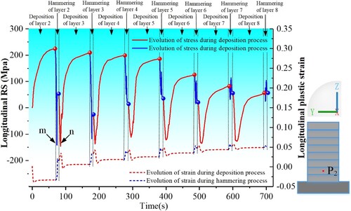
It can be seen from Figure 30 that the deposition of layer 2 generated longitudinal tensile stress with 221 Mpa and induced longitudinal compressive plastic strain in layer 2. However, the tensile plastic strain induced by the hammering of layer 2 mitigated the longitudinal compressive plastic strain in layer 2, and the longitudinal stress reduced from 221 Mpa to 53 Mpa. Subsequently, the longitudinal compressive plastic strain introduced by the deposition of layers 3–7 reduces the longitudinal tensile plastic strain of layer 2 and regenerates the longitudinal tensile stress of layer 2, but the accompanied hammering-induced tensile plastic strain reduces the tensile stress. By observing the longitudinal stress values in layer 2 after each layer deposition, it can be observed that the tensile stress generated by each subsequent layer deposition in layer 2 gradually decreased. On the other hand, the stress of layer 2 after the hammering of each layer initially increased and then decreased. During the hybrid process of layer 8, the stress of layer 2 tended to remain constant and the plastic strain hardly changed, this is because the deposition or hammering had minimal effect on the strain of layer 2. Compared to the longitudinal tensile RS generated by the deposition of layer 2, the RS of layer 2 reduced from 221 MPa to 56 MPa after the hammering of layer 8, and the longitudinal plastic strain level changed from compression (After the deposition of layer 2) to tension.

In addition, m and n instantaneous peak compressive stress shown in Figure 30 appeared in the hybrid process. The generation of m was affected by the hammering elastic strain generated, resulting in a short-term high-compression longitudinal stress level of −140 Mpa. With the recovery of elastic strain, the longitudinal stress rises to a 53 Mpa level. Subsequently, compressive longitudinal stress of −150 Mpa was generated during the deposition of layer 3. This is because the region where the heat source is located is heated dramatically. Due to the thermal expansion of the heated material, and constraints by the surrounding material, compressive stress is generated in front of the heated region. When the heat source passes through, the heated material will cool down in a short time. Due to the shrinkage of the heated material, the tensile stress is generated in the region behind the heat source [2]. Similar changes were also captured during the subsequent hybrid processes.

3.4. Mitigation of inter-layer hammering on ADED wall warping

Figure 31a, b shows the warping distribution of the deposition wall predicted by models 1 and 2 after removing the clamps. Along the Y-axis, it was observed that minimal warping occurred in the central region of the substrate, and the magnitude of warping was almost 0. The maximum warping was observed at both ends of the substrate, with a magnitude of 0.2 mm. As shown in Figure 31a, the distribution of warping magnitude exhibited a parabolic shape in the Y direction. The warping of the wall is similar to that of the substrate, a significant warping with 0.2 mm is observed at both ends. Figure 31b shows the suppression effect of inter-layer hammering on wall warping, it completely suppressed the warping in the building direction. The middle section bent upwards by 0.13 mm after removing the clamps.

Figure 31. The warping of the wall after removing the clamps: (a) ADED alone (model 2 predicts), (b) ADED hybrid inter-layer hammering (model 1 predicts).

4. Discussion

4.1. Longitudinal stress and plastic strain in ADED wall during a single inter-layer hammering process

Without considering the ADED process, the results of Section 3.2 show that the longitudinal tensile plastic strain is generated in the wall under the action of hammering. A longitudinal compressive plastic stress is generated in the wall to maintain the balance state. In contrast, the longitudinal tensile plastic strain introduced by the hammering at the top of the wall is much greater than the core of the wall, but the top of the wall produces a large longitudinal tensile stress. The same phenomenon is observed in the hybrid process. Ding et al. [2] attributed the generation of tensile stress region on the top of the ADED wall to the compressive plastic deformation at the end of the wall. The longitudinal tensile stress region near the wall top in the middle of the wall was not explained. By extracting the evolution of longitudinal strain at the top (Figure 26a) and core (Figure 26b, c, d) of the wall, it is found that the effect of hammering on the plastic strain of the top and core is different, and this difference can lead to tensile stress in the tensile plastic strain region at the top of the wall. According to the distribution of plastic strain in Figure 26, hammering causes a tendency for the material of the wall top to compress towards the hammering centre, while the region directly below the hammering action causes a tendency for the material to stretch lengthwise. which exacerbates the extrusion between materials. When studying the deformation in the welding process, Withers et al. [32] proposed that the RS is caused by the ‘misfit’ between regions caused by the thermal expansion of the material. The extrusion between the top materials of the wall caused by hammering can exacerbate the ‘misfit’ between the regions represented by the inspection points and result in tensile stress.

4.2. Evolution of longitudinal stress in ADED wall during the hybrid process

4.2.1. Characteristics of stress evolution

During the hybrid process of layers 2 and 3, the stress near the top of the wall was changed considerably. There was a phenomenon where the compressive stress generated by hammering completely covered the tensile stress generated by subsequent deposition or the opposite. The reduction of hammering on the longitudinal tensile stress was not retained. However, the longitudinal stress of the second layer is significantly reduced after the hammering of layer 7 (as shown in Figure 28c). An interaction theory between deposition and hammering was proposed to understand the stress evolution in the wall during the hybrid process. This interaction theory was created and generalised based on the stress evolution of the second deposition layer in Figure 28. It can describe the stress evolution characteristics of most deposition wall manufacturing processes. Distinct hues were employed to indicate the longitudinal stress levels throughout the hybrid process. The red region (Figure 32 a) indicates the generation of high longitudinal tensile stress after the deposition of layer N. Subsequently, the region longitudinal stress mitigation can be classified into two regions after the hammering of layer N (Figure 32b): the region of stress reduction ${\mathrm{H}}_0$ and the region beyond the range of hammering mitigation. Affected by the deposition of layer N+1 (Figure 32c), the region of stress reduction H₀ can be partitioned into two subdomains (H₁ and H₂). The region H₁ is near the top of the wall, the mitigation of the hammering of layer N on H₁ region stress is eliminated and the tensile stress is regenerated under the influence of layer N+1 deposition. In the region far away from the top of the wall (H₂), the migration effect of hammering on tensile stress was retained. Affected by the hammering of layer N+1 (Figure 32d), the tensile stress of region H₁ has been mitigated again, and region H₂ was further mitigated.

Figure 32. Characteristics model of ADED and inter-layer hammering interaction.

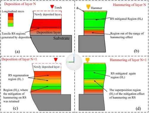
The hybrid process can be seen as a continuous cycle of the evolutionary process shown in Figure 32. The hammering continuously reduces the tensile stress introduced by the deposition in the region H₁, and when a newly deposited layer is deposition, this mitigation effect on tensile stress is eliminated by the deposition, then keep circulating. At the same time, the mitigation effect of hammering on tensile stress in region H₂ continues to accumulate, although each deposition weakens the accumulation effect. As the hybrid process proceeds. newly deposit layers were deposition, the region H₁ gradually far away from the location of deposition and hammering, and less affected by the influence than before, hence, the mitigation effect of hammering on tensile stress was not completely eliminated by subsequent deposition, i.e. the mitigation effect of hammering on tensile stress can be retained and then accumulated. The characteristics of stress evolution in the hybrid process can be summarised as follows: In the regions where far from the current deposition and hammering region (Like H₂), the mitigation effect of hammering on longitudinal RS will not be completely eliminated by deposition because the effect of deposition is small. In the near the current deposition and hammering region (Like H₁), due to the effects of deposition eliminate the mitigation effect of hammering on RS and regenerate tensile stress in these regions. As the hybrid process proceeds, the mitigation effect of hammering on longitudinal RS can be retained after several layers of deposition because the effect of deposition is reduced.

4.2.2. Dynamic evolution of stress distribution in ADED wall under the intersection of the deposition and hammering

Without considering the subsequent hybrid processes, the hammering of layer 2 (Figure 29a) is equivalent to post-deposition hammering, and it can be found that the ‘best mitigation position’ in longitudinal RS is observed to be at 2 mm from the surface of the substrate. However, when the subsequent multi-layer hybrid process is introduced, the ‘best mitigation position’ continuously changes. Under the influence of the deposition and hammering of layer 3, the best mitigation position shifts to 3.7 mm away from the surface of the substrate (Figure 29b). After the hammering of layers 6 and 7, the ‘best mitigation position’ is changed to 6 and 7 mm from the substrate surface, and the widths are 3 and 4.5 mm, respectively. The interaction of deposition and hammering is responsible for the variation of the‘best mitigation position’. The stress of the ADED wall will regenerate under the influence of deposition. The deposition of newly deposited layers leads to the impact position of the hammer rising in the Z direction, while the peak of the longitudinal compressive stress introduced by hammering occurs at 3 mm from the wall top (Section 3.2.1). The change in distance cannot allow the hammering to reduce stress in the same position by a constant mitigation effect, resulting in the distance between the ‘best mitigation location’ and the substrate surface being increased. In addition, the ‘best mitigation position’ changed from a single point position (Figure 29a) to a range (Figure 29d). The widening of the ‘best mitigation position’ range indicates that the stress in the ADED wall is affected by multi-round inter-layer hammering and the mitigation effect of hammering on longitudinal tensile RS continuously accumulates. This change is shown in the RS distribution curve as a distribution of low-level longitudinal stress (Figure 29d).

4.2.3. Dynamic evolution of local stress evolution in ADED wall under the interaction of deposition and hammering

It can be seen in Figure 30 that the compressive plastic strain induced by deposition is mitigated by the tensile plastic strain introduced by hammering and reduces the tensile RS in the wall. This is consistent with the results of the introduction of tensile plastic strain by single-layer hammering in section 3.2.1. The subsequent deposition continuously regenerated the longitudinal tensile stress of the wall and induced the longitudinal compressive plastic strain. However, the change amount of tensile plastic strain introduced by hammering was greater than that induced by the deposition, ensuring the accumulation of tensile plastic strain and the stress reduction in layer 2. The longitudinal stress evolution during the hybrid process (Figure 30) demonstrates that the influence of the deposition and hammering of each layer has a certain depth, i.e. the longitudinal stress and longitudinal plastic strain in the layers underneath the top surface are changed by the deposition or hammering, and the influence depth can be indicated by the number of deposition layers between the layer 2 and the active surface of deposition or hammering. During the deposition of layer 8, the deposition has little effect on the plastic strain of the layer 2. The plastic strain difference caused by the deposition of layer 7 and layer 8 in layer 2 is less than 0.005, and the deposition of layer 8 had almost no influence on the longitudinal RS in layer 2(Compared to the RS after the hammering of layer 7). Hence, the distance from layers 2 to 8 (i.e. layers 2-8) is thus considered as the depth of deposition influence.

From the evolution of layer 2 longitudinal RS and plastic strain during the hybrid process, the plastic strain level in layer 2 stabilised after the hammering of layer 7, and the hammering of layer 8 changed the plastic strain of layer 2 by less than 0.001. In contrast to the longitudinal stress levels in layer 2 after the deposition of layer 8 and hammering of layer 8, there was no change in the longitudinal stress in layer 2 after the hammering of layer 7. Thus, the depth of hammering influence is the distance from layers 2 to 7. The value of influence depth was slightly deeper than predicted by model 3. This shows that it is necessary to build a hybrid model to predict the mitigation effect of inter-layer hammering on RS. Compared with the stress predicted by model 2, the final longitudinal RS in layer 2 reduced from 221 MPa to 56 MPa.

5. Conclusions

In this paper, the ADED hybrid inter-layer hammering finite element model was developed based on the ‘result cyclic transfer’ and ‘surface mesh extraction and reconstruction’. The hybrid model was verified from four aspects: heat input, ADED wall section morphology, warping of the substrate, and the RS. The distribution of plastic strain and stress of a single inter-layer hammering was used as the basis for studying the evolution of plastic strain and stress during the hybrid process. In the hybrid process, the change amount of hammering-introduced plastic strain was greater than deposition-introduced, which ensures the accumulation of tensile plastic strain in the deposition layer. An intersection theory is proposed and universalised to explain the evolution characteristics of stress during the hybrid process. Finally, the concurrent evolution of local stress and strain in the hybrid process reveals the influence range of deposition and hammering. The following conclusions are drawn:

1. The longitudinal stress of the deposition layer was influenced by the subsequent six layers of inter-layer hammering. Compared with the RS predicted by model 2 (ADED alone), the RS value reduced by 74.6% from 221 MPa to 56 MPa.

2. During the hybrid process, the magnitude of the hammering-introduced tensile plastic strain is greater than that of the deposition-introduced, which ensures the accumulation of tensile plastic strain and stress reduction in the ADED wall.

3. After a single inter-layer hammering, the tensile stress at the wall top rapidly changes to compressive stress along the negative direction of the building, and the compressive stress exhibits an increasing trend from the top of the wall, reaching its maximum of −30 Mpa at a position of 3 mm away, and then gradually decreases. After seven hybrid processes, a low-stress distribution with an average value of 10Mpa was formed in the range of the ADED wall 6.5-11 mm from the substrate surface.

4. According to the characteristics of stress evolution in interaction theory, a more effective RS reduction strategy of the ADED wall needs to consider how to better retain the stress reduction effect of hammering in regions far away from the current deposition position.

5. The distribution of longitudinal plastic strain introduced by hammering at the ADED wall top and wall centre is different. The hammering-introduced plastic strain at the wall top can exacerbate the ‘misfit’ between the top regions of the wall. This leads to longitudinal tensile stress in the longitudinal tensile plastic strain region at the top of the wall.

Disclosure statement

No potential conflict of interest was reported by the author(s).

Data availability statement

The data that support the findings of this study are available from the corresponding author, upon reasonable request.

Additional information

Funding

This work was supported by the National Key Research and Development Program of China [Grant No. 2022YFB4602201], National Natural Science Foundation of China [Grant No.52005351], China Postdoctoral Science Foundation [Grant No. 2022M722993], Shenyang Youth Science and technology innovation project [Grant No. RC220449] and Basic Scientific Research Project of Liaoning Provincial Department of Education [Grant No. LJKQZ2021160].

References

- Williams SW, Martina F. Wire+ air additive manufacture[J]. Materials Science And Technology, IoM, Bedford, England; 2015.
- Ding J. Thermo-mechanical analysis of wire and arc additive manufacturing process[D]. Cranfield, Bedfordshire: Cranfield University; 2012.
- Brust FW, Kim DS. Mitigating welding residual stress and deformation[M]//Processes and mechanisms of welding residual stress and deformation. Woodhead Publishing; 2005:264–294. doi:10.1533/9781845690939.2.264
- Mughal MP, Mufti RA, Fawad H. The mechanical effects of deposition patterns in welding-based layered manufacturing[J]. Proc Inst Mech Eng, Part B: J Eng Manuf. 2007;221(10):1499–1509. doi:10.1243/09544054JEM783
- Chigilipalli BK, Veeramani A. An experimental investigation and neuro-fuzzy modeling to ascertain metal deposition parameters for the wire arc additive manufacturing of Incoloy 825[J]. CIRP J Manuf Sci Technol. 2022;38:386–400. doi:10.1016/j.cirpj.2022.05.008
- Sun L, Ren X, He J, et al. A bead sequence-driven deposition pattern evaluation criterion for lowering residual stresses in additive manufacturing[J]. Addit Manuf. 2021;48:102424. doi:10.1016/j.addma.2021.102424
- Gornyakov V, Ding J, Sun Y, et al. Understanding and designing post-build rolling for mitigation of residual stress and deformation in wire arc additively manufactured components[J]. Mater Des. 2022;213:110335. doi:10.1016/j.matdes.2021.110335
- Shen H, Lin J, Zhou Z, et al. Effect of induction heat treatment on residual stress distribution of components fabricated by wire arc additive manufacturing[J]. J Manuf Process. 2022;75:331–345. doi:10.1016/j.jmapro.2022.01.018
- Goviazin GG, Rittel D, Shirizly A. Achieving high strength with low residual stress in WAAM SS316L using flow-forming and heat treatment[J]. Mater Sci Eng A. 2023;873:145043. doi:10.1016/j.msea.2023.145043
- Colegrove PA, Coules HE, Fairman J, et al. Microstructure and residual stress improvement in wire and arc additively manufactured parts through high-pressure rolling[J]. J Mater Process Technol. 2013;213(10):1782–1791. doi:10.1016/j.jmatprotec.2013.04.012
- Martina F, Roy MJ, Szost BA, et al. Residual stress of as-deposited and rolled wire+ arc additive manufacturing Ti–6Al–4 V components[J]. Mater Sci Technol. 2016;32(14):1439–1448. doi:10.1080/02670836.2016.1142704
- Colegrove P A, Martina F, Roy MJ, et al. High pressure interpass rolling of wire+ arc additively manufactured titanium components[J]. Adv Mat Res. 2014;996:694–700. doi:10.4028/www.scientific.net/AMR.996.694
- Abbaszadeh M, Hönnige JR, Martina F, et al. Numerical investigation of the effect of rolling on the localized stress and strain induction for wire+ arc additive manufactured structures[J]. J Mater Eng Perform. 2019;28:4931–4942. doi:10.1007/s11665-019-04249-y
- Gornyakov V, Sun Y, Ding J, et al. Computationally efficient models of high pressure rolling for wire arc additively manufactured components[J]. Appl Sci. 2021;11(1):402. doi:10.3390/app11010402
- Gornyakov V, Sun Y, Ding J, et al. Modelling and optimizing hybrid process of wire arc additive manufacturing and high-pressure rolling[J]. Mater Des. 2022;223:111121. doi:10.1016/j.matdes.2022.111121
- Tangestani R, Farrahi GH, Shishegar M, et al. Effects of vertical and pinch rolling on residual stress distributions in wire and arc additively manufactured components[J]. J Mater Eng Perform. 2020;29(4):2073–2084. doi:10.1007/s11665-020-04767-0
- Zhou S, Wang J, Yang G, et al. Periodic microstructure of Al-Mg alloy fabricated by inter-layer hammering hybrid wire arc additive manufacturing: Formation mechanism, microstructural and mechanical characterization[J]. Mater Sci Eng A. 2022:144314. doi:10.1016/j.msea.2022.144314
- Jin W, Zhang C, Jin S, et al. Wire arc additive manufacturing of stainless steels: a review. Appl Sci. 2020;10:1563. doi:10.3390/app10051563
- Lin Z, Song K, Yu X. A review on wire and arc additive manufacturing of titanium alloy[J]. J Manuf Process. 2021;70:24–45. doi:10.1016/j.jmapro.2021.08.018
- Derekar KS, Ahmad B, Zhang X, et al. Effects of process variants on residual stresses in Wire Arc additive manufacturing of Aluminum Alloy 5183[J]. J Manuf Sci Eng. 2022;144(7). doi:10.1115/1.4052930
- Asala G, Khan AK, Andersson J, et al. Microstructural analyses of ATI 718Plus® produced by wire-ARC additive manufacturing process[J]. Metall Mater Trans A. 2017;48(9):4211–4228. doi:10.1007/s11661-017-4162-2
- Kalpakjian S. Manufacturing engineering and technology[M]; 1995.
- Goldak J, Chakravarti A, Bibby M. A new finite element model for welding heat sources[J]. Metall Trans B. 1984;15(2):299–305.
- Fang X, Zhang L, Yang J, et al. Effect of characteristic substrate parameters on the deposition geometry of CMT additive manufactured Al-6.3% Cu alloy[J]. Appl Therm Eng. 2019;162:114302. doi:10.1016/j.applthermaleng.2019.114302
- Fitzpatrick ME, Fry AT, Holdway P, et al. Determination of residual stresses by X-ray diffraction[J]; 2005.
- Krawitz AD, Brune JE, Schmank MJ. Residual stress and stress relaxation[J]. Kula and V. Weiss eds, 1982: 139.
- Cullity BD. Elements of X-ray Diffraction[M]. Boston, Massachusetts: Addison-Wesley Publishing; 1956.
- Teixeira V, Andritschky M, Fischer W, et al. Effects of deposition temperature and thermal cycling on residual stress state in zirconia-based thermal barrier coatings[J]. Surf Coat Technol. 1999;120:103–111. doi:10.1016/S0257-8972(99)00341-2
- Zhang W, Guo D, Wang L, et al. X-ray diffraction measurements and computational prediction of residual stress mitigation scanning strategies in powder bed fusion additive manufacturing[J]. Addit Manuf. 2023;61:103275. doi:10.1016/j.addma.2022.103275
- Muhammad NA, Geng P, Wu CS, et al. Unravelling the ultrasonic effect on residual stress and microstructure in dissimilar ultrasonic-assisted friction stir welding of Al/Mg alloys[J]. Int J Mach Tools Manuf. 2023;186:104004. doi:10.1016/j.jallcom.2023.169315
- Luo Q, Jones AH. High-precision determination of residual stress of polycrystalline coatings using optimised XRD-sin2ψ technique[J]. Surf Coat Technol. 2010;205(5):1403–1408. doi:10.1016/j.surfcoat.2010.07.108
- Withers PJ, Bhadeshia H. Residual stress. Part 2–Nature and origins[J]. Mater Sci Technol. 2001;17(4):366–375. doi:10.1179/026708301101510087