Land-use conversions from managed grasslands to croplands in Uruguay increase medium-term net carbon emissions to the atmosphere

ABSTRACT

Globally, significant land conversions of traditionally managed temperate grasslands to croplands were taking place. Among these is South-Central Uruguay where changes in recent decades have highly likely impacted plant productivity, soil quality, and carbon fluxes at a regional scale. A geospatial version of the biophysical model EPIC was developed and validated (Geospatial-EPIC-UY). An analysis of the potential impact of the land use change on the carbon fluxes was performed, considering the conversion of all the suitable cropping areas over a 15-year period. Modeled net ecosystem exchange (NEE) showed that, on average, grasslands C emissions were close to neutral (0.1 Mg CO₂ ha⁻¹ year⁻¹), while croplands contributed almost 7 times this value. Also, the inter-annual variation of grassland NEE was significantly less than that of the cropland. These results highlight the potential C losses under extended land conversions, which could be attenuated or even reverted if best management practices were implemented.

KEYWORDS:

• Carbon fluxes
• NPP
• NEE
• soil carbon
• carbon dynamics
• natural grassland ecosystem
• cropland ecosystem
• epic model
• regional scale
• uruguay

1 Introduction

For decades, there has been worldwide land use conversion (LUC) of natural grassland to cropland ecosystems to increase farm profits and satisfy ever-increasing demands for food, feed, and fiber. This conversion from grassland to cropland ecosystems is mostly achieved using tillage implementations to prepare seedbeds, control weeds and apply nutrients. Often, tillage disturbance enhances soil organic matter oxidation, enhancing soil carbon emissions to the atmosphere, destroying soil structure, and accelerating soil erosion, thereby reducing soil quality, crop productivity, and provision of ecosystem services (Lal, 2002).

Globally, beyond the need for soil degradation assessments, there is also an urgent need to better quantify carbon budgets and fluxes (stock, sequestration and emissions) of managed ecosystem conversions at different scales: field, regional, national, and global (IPCC, 2003). At a global scale, carbon fluxes resulting from LUC are being estimated by book-keeping models and coarse resolution dynamic global vegetation models (R. A. Houghton & Nassikas, 2017; Richard A. Houghton, 2018). At a national scale, local calibrated and adapted process-based models providing spatially and temporally explicit estimations are required to fulfill the National Reports of greenhouse emissions under the United Nations Framework Convention on Climate Change (UNFCCC) and Kyoto Protocol using IPCC ‘Tier 2’ or ‘Tier 3’ methodologies (IPCC, 2003) and also to provide scientific basis to develop sustainable land use policies at a country level (Sohl et al., 2012; Tiemeyer et al., 2020).

Temperate grasslands, a major type of grasslands, account for a large fraction of the Earth’s vegetation (Coupland, 1992). Large expanses of temperate grasslands and derivative croplands are located particularly in the mid-latitudes in Asia, North America, and South America (Sala et al., 1996). In South America, temperate grasslands occupy large areas. The Pampa grasslands alone are one of the largest temperate grassland regions in the world, occupying over 700,000 km² across eastern Argentina, Uruguay, and southern Brazil (Soriano et al., 1992). This region, the most extensive biogeographic unit of the prairie biome in South America, has been extensively modified by human activities (Guerschman et al., 2003). Currently, it contributes significantly to the domestic and international trades of crop commodities, thereby inducing extensive and intensive changes in land use and cover (Altesor et al., 2006; Vega et al., 2009) and, in so doing, affecting carbon cycling and ecosystem properties.

Uruguay, in contrast with other regions, still has a high percentage of grasslands, which are therefore vulnerable to land use change. During 1999–2010, Uruguay expanded its cropland area from 200,000 to >1,000,000 ha, mainly due to soybean (Glycine max (L.) Merr.) and wheat (Triticum aestivum L.) cropping (MGAP Uruguay, MVOTMA Uruguay & FAO, 2011). During the same period, the area under grassland cover decreased from 67.4% to 61.4% (MGAP-DIEA, 2016a). This process mainly took place in the South-Central Uruguay region (Baeza & Paruelo, 2020). However, a quantification of the intensity and extent of the potential impacts of the land use and management changes on soil quality and carbon cycling is currently lacking.

At present, there is a scarcity of systematic and extensive collection of field data of C budget and fluxes and spatial estimations. Smith et al. (2012) suggested using process-based agroecosystem models to provide these essential measurements. In this study, the EPIC (Environmental Policy Integrated Climate) model was selected to simulate key agroecological processes associated with grassland-cropland conversions such as plant growth, plant yield, water balance, soil erosion, soil carbon dynamics, nutrient cycling, and greenhouse-gas emissions (Izaurralde et al., 2006; Williams et al., 1984). The EPIC model (Williams et al., 1984) has been used elsewhere to simulate C fluxes, for example, US cropland regions (Causarano et al., 2008; Izaurralde et al., 2007; Zhang et al., 2015) and other regions of the world (Apezteguía et al., 2009; Billen et al., 2009). Previous studies in Uruguay used the Century model (Baethgen, 2003; Parton et al., 1988), but it does not explicitly simulate land degradation processes such as soil erosion as needed for this study (Baethgen, 2003; Caride et al., 2012).

The objectives of this research were to i) Develop and test a spatial data-modeling system to simulate field-scale crop productivity and soil processes under grassland and cropland covers in South-Central Uruguay (Geospatial-EPIC-UY) achievable through the point-scale calibration and testing using local data and by developing a spatial version of the model adapted to Uruguayan agroecosystems and ii) address the potential C-flux impacts of the Land Use (LU) change if all the suitable areas to grow crops where converted from grassland to cropland. To our knowledge, this is an original contribution to simulate grassland productivity and carbon fluxes under conditions of LU change in the Rio de la Plata grasslands.

2 Materials and methods

2.1 Study area

Uruguay is in the southeast of South America, between 30º and 35º South and 54º and 59° West. The total land area is 176,215 km². The region is dominated by rolling plains with a maximum elevation of 514 m. The climate is temperate, with a range of rainfall between 1,100 and 1,300 mm yr⁻¹, mean temperatures of 11°C in the winter and 27°C in the summer, and extreme temperatures of – 4°C and 40°C (Castaño-Sánchez et al., 2011). The main ecosystem is grassland associated with riparian bush forest. Soils are slightly acidic Prairie Soils (Mollisols) (Berretta, 2003). The ‘Southern Campos’ sub-region (Soriano & Paruelo, 1992) was selected as the study area (Figure 1); it is located in the center-south of Uruguay where soils support natural grassland and has limited crop use capabilities (MGAP-RENARE-DSA, 2003). Our objective was to quantify the potential impacts of LU change considering only soil units deemed suitable for growing cash crops (Figs. S2 and S10). Soil units were selected using the crop suitability classification (suitable, less suitable, marginal, and not suitable) made by MGAP-RENARE-DSA (2003) at scale 1:40,000 scale (MGAP-DGRNR-CONEAT, 1994).

Figure 1. Map of the study area showing the main categories of LULC in 2010 (MGAP Uruguay, MVOTMA Uruguay & FAO, 2011). Inserted map of South America, showing the study area (green zone)

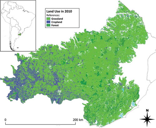
Currently, the Uruguayan agroecosystem is composed of two main sub-systems, which usually co-exist in the same farm: a) Natural Grasslands and b) Croplands. The Natural Grassland sub-ecosystem is characterized by domestic bovine and ovine herbivores, grazing together on the evolved natural pasture. Productivity averages 3–4 Mg DM ha⁻¹ yr⁻¹. The managed grassland consists of a consociation of grasses, herbs, and shrubs, with the presence of few if any trees. It is rich in biodiversity (>400 grass species) with a high proportion of summer species (C₄) in comparison to winter species (C₃). Perennials dominate over annual species. However, of this great diversity of species, only 10 are the main contributors to the annual forage production (Berretta, 2003). The pastures are grazed by the livestock continuously year-round without mowing, and the livestock rate or density is moderate averaging 0.6 LSU ha⁻¹ [LSU: Live Stock Units (EUROSTAT, 2013)] and remains mostly fixed across years (Fig. S12) and within the year (MGAP-DIEA, 2016b).

The Cropland sub-ecosystem consists of a rainfed crop production system. On average, farms are 775 ha in size and are privately owned. And a high proportion is rented under short-term contracts (MGAP-DIEA, 2016a). About half of the crop area is under a summer-winter rotation while the other half is under a summer-summer rotation. The main crops are soybean in the summer and wheat in the winter, both produced with no-tillage (MGAP-DIEA, 2016a). In the study area, the main winter crop is wheat and the main summer crop is soybean followed by sorghum (Sorghum bicolor (L.) Moench).

2.2 Description of the EPIC model and inputs

The Environmental Policy Integrated Climate (EPIC) Model is a cropping systems simulation model originally developed in the 1980s to estimate the effects of erosion on soil productivity throughout the United States (Williams et al., 2008, 2006). Since then, EPIC has evolved into a comprehensive agro-ecosystem model capable of simulating the growth of crops grown in complex rotations and management operations, such as tillage, irrigation, fertilization and liming (Izaurralde et al., 2006). EPIC has been continually improved through the addition of algorithms to simulate nitrogen, carbon, and phosphorus cycling, water quality, the effect of atmospheric CO₂ concentration and climate changes (Izaurralde et al., 2012). The model operates at field/small watershed scale at daily time steps simulating soil erosion, nutrient balance, crop growth, and related processes. Fig. S1 shows the schematic of the modeling steps with its main inputs, components/processes and outputs. The EPIC version 1102 was used in this research (Williams et al., 2006).

The main sub-models/processes of EPIC pertaining to this research include the crop and the soil carbon-nitrogen sub-model. A single plant growth model is used to simulate about 100 plant species, each using a unique set of parameter values. These include crops (annual and perennial), native grasses, and trees. The coupled soil carbon-nitrogen (C:N) sub-model (Izaurralde et al., 2006) follows the approach used in the Century model (Parton et al., 1988), where C and N in soil organic matter are distributed among three pools: active (microbial), slow and passive. The pools differ in size and function and have turnover times ranging from days to hundreds of years (Izaurralde et al., 2006).

The EPIC model has been widely used for assessing the effects of management on erosion, soil productivity and soil C dynamics, in a wide range of environments and agricultural systems, e.g. North America (Causarano et al., 2008; Izaurralde et al., 2012; Roloff et al., 1998), Europe (Balkovič et al., 2013; Billen et al., 2009; Farina et al., 2011), Asia (Causarano et al., 2011; Ma et al., 2016), South America (Apezteguía et al., 2009; Bernardos et al., 2001; Gaiser et al., 2010) and Africa (Adejuwon, 2005; Freier et al., 2011).

2.3 Development and validation of the Geospatial-EPIC-UY

Even though EPIC is flexible enough to perform under a variety of environments, there was no prior experience using the model to simulate the Uruguayan agroecosystem. Consequently, there was a need to calibrate and validate the model, first at a field scale and then at a regional scale.

2.3.1 Field-scale EPIC calibration and validation

The calibration process followed the guidelines provided in the EPIC user’s guide (Williams et al., 2006). It includes successive modifications of the model parameters using the weather, soils, land use and agronomic conditions of the study area until an acceptable reproduction of observed biophysical processes is achieved (Bernardos et al., 2001). The calibration was performed independently for the grassland and the cropland ecosystems because these have very different vegetation, management and development conditions following the guidelines provided in the EPIC user’s guide (Williams et al., 2006). Site descriptions and sources of data for field calibration are given in Tables S1 and S2.

Since the plant-C input is the main driver of soil C dynamics (Apezteguía et al., 2009), as a first step in the calibration process, it was important to confirm that the EPIC crop growth module (Gassman et al., 2005) correctly simulated the annual C inputs to the soil. Second, to address the complete C cycle, we tested the ability of EPIC to reproduce field observations of soil organic carbon. Model performance, when replicated observational data were available, was measured with two standard statistical tests: 1) t-test to evaluate the probability that modeled and observed values were the same and 2) regression analysis to test if the modeled and field data were correlated (statistical significance of the coefficient of determination and the regression slope).

Simulation of the grassland ecosystem

First, we focused on the model calibration of grass forage yields by comparing historical yearly and seasonal yield averages with outputs from model runs using a representative soil profile of the study area and 30 years of daily weather data (Table S2). A grass species from the crop database available in EPIC was selected and adapted to simulate the ‘Grassland Uruguay crop’. After testing different summer, winter and combination of both grasses available in EPIC, we selected ‘Summer grass crop’ as a foundation since Uruguayan grassland is dominated by summer grasses, with a C₄ photosynthetic pathway (Berretta, 2003). To reflect the characteristics of the dominated species in the study area, we manually modified the crop parameters based on previous published procedures (Adejuwon, 2005; Causarano et al., 2008) (Table S3). Although the EPIC has a grazing routine, the best option was to employ a simulated grazing approach using available EPIC’s operations and detailed grazing calculations based on published data, which is presented in detail in the supplemental information (Appendix S3). After calibration, we validated the modeled forage yield with field data measured yearly and seasonally from two sites (INIA-TyT-RS and SUL-CC-RS) undergoing continuous cattle grazing (Tables S1 and S2, Fig. S2). We tested the model’s capability to reproduce soil carbon dynamics as affected by residue additions, microbial respiration, and carbon losses with soil sediments, runoff, and leaching, against measured soil carbon in one of the grassland experiments previously used to validate the forage yield (INIA-TyT-RS) where the data consisted of yearly measurements of soil carbon to 15-cm depth (Table S1 and S2).

Simulation of the cropland ecosystem

As described above, the cropland ecosystem consisted of a rotation of winter and summer crops. We selected a 2-year rotation sequence of three crops: spring wheat, soybean and sorghum, which allows a sustainable crop production in the study region (Terra et al., 2006). The rotation consists of (a) spring wheat planted in late autumn, harvested in late spring; (b) soybean planted immediately after wheat harvest and harvested in early autumn; (c) spring wheat planted in late autumn, harvested in late spring, and (d) sorghum planted in late spring and harvested in mid-autumn. Thus, we performed the model calibration on three crops: spring wheat, soybean and sorghum, following the general modeling procedures as described by Causarano et al. (2007) and Apezteguía et al. (2009).

Similar to the process applied to calibrate the grassland system, the first step was to simulate the three crops using historical weather data over a period of 15 years, and we focused on achieving representative crop grain yields comparable to historical yearly national statistics data (MGAP-DIEA, 2015) and reproducing the crop cycle characteristics of the three crops (Castro et al., 2015). During this stage, the parameters of the three crops in the EPIC crop database were modified manually based on previous research (Causarano et al., 2007) and the characteristics of the Uruguayan cropland management (planting date, plant population, fertilization, etc.) (Table S4). To obtain a better adjustment, a second, automatic calibration was conducted using a parameter optimization algorithm (HydroPSO package; Zambrano-Bigiarini & Rojas, 2013) from the R statistical software package (R Development Core Team, 2013). This package implements a modified version of the Particle Swarm Optimization (PSO) algorithm which optimizes based on a user-defined goodness-of-fit measure until a maximum number of iterations or a convergence criterion are met (Zambrano-Bigiarini & Rojas, 2013). We selected and adjusted five EPIC parameters in this process (Table S5). To conduct the automatic calibration, we used the first 6 years (2003–2008) of measured grain yield and crop management data (Table S4) from a 10-year crop variety trial experiment (INIA-LE-RS, Table S2 and Fig. S2). We selected these available experimental data because in our study region, the grain yields of these trial experiments were similar to those of farmers from good managed crop yields in high crop aptitude soils (AUSID, 2009, 2010), and based on similar research where Sharda et al. (2020) on a regional simulation of maize yields in the USA found that field trials were deemed a valid option when lack of farm field data was available. Moreover, contrasting environments were present during the first 6 years (Fig. S11), thus allowing for a more robust calibration.

We performed the validation of modeled crop grain yields with data not used previously during the calibration of the INIA-LE-RS experiment (4 years, 2009–2012) and from two other sites: first, ten-year crop variety trial experiment (INIA-SRRN, Table S2), which is an independent dataset replicating the experiment used for calibration under slightly different agro-ecological conditions (Figs. S11) located 200 km north (Figs. S2) and second, a six-year no-tillage farm-scale crop rotation experiment (year 1 – wheat-soybean, year 2 – wheat-sorghum) conducted with crop management and machines used by farmers located in soils with medium agricultural aptitude (INIA-TyT-RS, Table S2, Fig. S2) to evaluate if the calibrated model represents the crop yields in representative farm with medium soil aptitude. Currently, this crop rotation is not a common practice, but it is deemed as a sustainable crop production rotation in the study region. Finally, we tested the capability of EPIC to reproduce soil carbon dynamics in cropland systems by comparison with 15-cm depth soil carbon measured in the crop rotation experiment (INIA-TyT-RS, Table S2).

2.3.2 Development and validation of the EPIC model at regional scale

The development of a spatially explicit version of the EPIC model at the regional scale (Geospatial-EPIC-UY) includes the following steps: 1) building of a geospatial database with the required data (Table S6), 2) building of the Homogenous Spatial Modeling Units (HSMUs) and 3) building of faster computing environment using a parallel model-running environment.

2.3.2.1 Building of the Homogenous spatial modeling units (HSMU) and computing environment

As mentioned above, we only modeled the land suitable for growing cash crops, as indicated by MGAP-RENARE-DSA (2003) (Figure 1). This cash-crop area, covering ~50% of the total study area, was assumed to be the maximum area that could potentially be dedicated to growing cash crops.

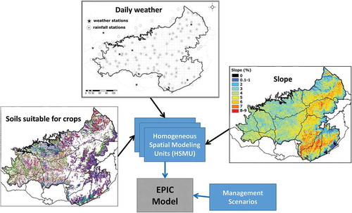
To build the homogenous spatial modeling units (HSMU), considering the maximum potential crop area, we adapted the approach presented by Zhang et al. (2010) to this region using the available data sources (Table S6). A conceptual diagram of the geospatial EPIC simulation system is presented in Figure 2. We used the polygons of the 1:40,000 soil map shapefile as a base, getting about 7,500 HSMUs (polygons). For each HSMU, we computed the spatial average of the Slope and Elevation from the digital elevation model (DEM) raster file; finally, we assigned a grid cell with daily weather data based on the proximity of both centroids (weather grid and HSMU polygon). The computing environment was a parallel version of EPIC implemented in Linux (Zhang et al., 2015) in order to reduce the run time that would be needed to simulate each HSMU in turn. Finally, the simulation results were extracted from the EPIC output using a script from R Statistics software (R Development Core Team, 2013).

Figure 2. Conceptual diagram of Geospatial-EPIC-UY. For description and source of data, see Table S6. Enlarged individual maps are provided in the online appendix (Fig. S3 and S4)

2.3.2.2 Spatial EPIC validation

Following the validation at a field scale and the development of the Geospatial-EPIC-UY for these conditions, the next step was to validate it for both agroecosystems with the available data at this scale.

Grassland ecosystem validation

Due to the lack of spatially distributed grassland forage yield field data, we conducted an indirect validation, by comparing for each HSMU the average of the modeled grassland forage production by the Geospatial-EPIC-UY over 15 years, with the CONEAT (acronym in Spanish of the National Commission for the Agronomic Study of Soils) Productivity Index (CONEAT PI). The CONEAT PI (Act 13.695; October 1968 of the Uruguayan government) is an index of the potential production capacity of the soils in terms of annual production of bovine meat, sheep meat, and wool per hectare. It was developed using an expert assessment approach by Uruguayan soil professionals, and the productivity value was assigned to 188 soil groups of the map scale 1:40.000 according to their similarities. The index values range from 0 (lowest) to 263 (highest) while the average value at a country scale is the index of 100 (Capurro Etchegaray, 1977). A detailed description of the origin and conceptual base and how the index and the cartography were made could be found in Lanfranco Crespo and Sapriza Fraga (2011). Despite having been developed almost 50 years ago, the index still captures well the current land productivity/capability, as confirmed by Lanfranco Crespo and Sapriza Fraga (2011) who found a positive correlation between the CONEAT PI and the unit price of farmland. We considered that this index could be used as an indirect measure of the grassland productivity since it is directly related to forage availability. Since they are in different units, the standardized values (z-value) of both were used (Rahman et al., 2009) and expressed as in Eq. (1)(1) $z_i=\frac{\left(x_i-{\mu }_i\right)}{{\sigma }_i}$(1) :

(1) $z_i=\frac{\left(x_i-{\mu }_i\right)}{{\sigma }_i}$(1)

where z_i is the standardized value for each soil group, x_i is the original value,${\mu }_i$ is the mean value of the population and ${\sigma }_i$ is the standard deviation.

Cropland ecosystem validation

We selected the soybean crop to validate the EPIC spatial model on croplands since its area is 90% of summer crops – almost double the winter crop area (MGAP-DIEA, 2015). In order to obtain a good representation of the crop productivity, we compared the average of the Geospatial-EPIC-UY annual yield outputs for the whole region with national crop yield averages (MGAP-DIEA, 2016b). Although these data are for an area larger than the study area, it covered 16 years, thus enabling a comparison of trends in inter-annual yield variability.

2.4 Potential changes in carbon fluxes

The net ecosystem exchange (NEE) is the net CO₂ flux between the terrestrial ecosystem and the atmosphere; a negative sign of NEE indicates C uptake into the biosphere, while a positive value denotes net emission to the atmosphere (Chapin et al., 2006). Recent studies (Schwalm et al., 2010; Zhang et al., 2015) showed that the C algorithm in EPIC acceptably simulated NEE of diverse agroecosystems in the US Midwest. NEE was calculated as heterotrophic soil respiration (RSPC) minus the net C sequestration (NPP) from the atmosphere into plant biomass (Chapin et al., 2006).

Here, we performed an analysis of the potential impact on the carbon fluxes of a hypothetical land use change of all the potential cultivable area from grassland to cropland on the carbon fluxes. For both, we ran the Geospatial-EPIC-UY over 15 years, extracting the pertinent variables (NEE, RSPC, NPP). The grassland was simulated for each HSMU as was described previously during the calibration/validation, considering that during the simulated period, the stocking rate is kept fixed (Fig. S12) grazing a proportion of the available forage (Appendix 3). The cropland was simulated as only soybean crop without rotation with other crops (soybean monoculture) considering that all the area was converted from grassland at the beginning of the 15-year period, where the grassland was chemically terminated with herbicide followed by the soybean planted with no-till. The focus was on the biogenic-related C processes included in the NEE calculation omitting fuel use and heterotrophic respiration by humans and livestock (West et al., 2011).

3 Results

3.1 Development and validation of UY-adapted GeoSpatial EPIC

3.1.1 Field-scale calibration and validation

Simulation of grassland ecosystem

We calibrated the model by comparing it with the historical yearly averages extracted from sparse bibliographic data sources (Table S2). During the calibration process, we manually modified the crop parameters to best mimic the observed forage yields (seasonal, yearly, inter-annual) to build the ‘Grassland Uruguay crop’, until the best adjustment of the model was achieved. The final values of these parameters are shown in Table S3. These results indicated that EPIC simulated well the mean response of historic, yearly, forage yields (Table 1). Furthermore, simulated maximum and minimum yearly yields agreed well with those recorded in dry and wet years (Castaño-Sánchez et al., 2011). In the seasonal representation, the model tended to overpredict yields somewhat in the summer and underpredict in the winter (Table 1).

Table 1. Results of field-scale grassland calibration and validation

Calibration
				Average of yearly results
Variable	Site	Period	Type	(Mg ha^−1) [minimum-maximum]				Seasonal distribution (percentage of yearly)
Forage	Representative soil and climate	1995–2015 (30 years)	simulated	3.56 [1.77–4.55]				27% SP, 51% SU, 20% FA, 2% WI
	Published across study region		measured	3.46 [1.19–5.25]				25–29% SP, 38–48% SU,19–23% FA, 9–13% WI
Validation
				Yearly results
Variable	Site	Period	Type	(Mg ha^−1)	Standard error	RMSE	correlation	Seasonal correlation
Forage	INIA-TyT-RS	1991–2003 (12 years)	simulated	3.55*	0.16	0.43	R^2 = 0.60**	R^2 = 0.69**
			measured	3.39*
Forage	SUL-CC-RS	1984–1990 (7 years)	simulated	3.09*	0.50	0.50	R^2 = 0.51**
			measured	3.24*
SOC loss	INIA-TyT-RS	2006–2012 (7 years)	simulated	−0.496*	0.48	1.08	R^2 = 0.72**
			measured	−0.446*

* difference not statistically significant between simulated and measured (T-Test, p < 0.05), ** significantly correlated (ANOVA, p < 0.05)

SP: Spring, SU: Summer, FA: Fall, WI: Winter

Next, we validated the modeled forage results on two sites (Table 1). Modeled mean forage annual yield at the two sites tested showed good agreement with measured yields (Table 1, Fig. S5a). There was also close agreement between seasonal yields (Fig. S5b and S5b) although the model overestimated the yield in the summer and underestimated it in the winter, repeating the trend during the calibration.

For the modeling of soil carbon changes, the simulated mean yearly C loss was close to the measured loss during the study period (Table 1). Analyzing the inter-annual behavior (Fig. S6), measured soil carbon was more variable than modeled ones, likely due to expected spatial variability and sampling errors. In spite of this, there were significant negative trends in both observed and simulated soil carbon.

Simulation of cropland ecosystem

As with the grassland, the first step of the model calibration process was to achieve the measured historical grain yield (national statistics, Table S2) and the length of the crop cycle (Table S2) of the three crops, manually modifying the EPIC´s crop parameters. After this process, we obtained a reasonable behavior of the model outputs, a realistic agreement of the length of crop cycle and an acceptable crop yield average, but the model was still overpredicted by more than 20% the measured yields that required a further step to improve it. During the automatic calibration using the HydroPSO package, with data from the INIA-LE-RS experiment (6 years), the best adjustment of the model was achieved with the values of the model parameters shown in Table S5. After this procedure, the agreement between modeled and measured crop yields was excellent, as could be observed in Table 2 and Fig. S7a.

Table 2. Results of field-scale cropland calibration and validation

Calibration
				Soybean	Wheat	Sorghum		Three crops
Variable	Site	Period	Type	(Mg ha^−1)	(Mg ha^−1)	(Mg ha^−1)	(Mg ha^−1)	Standard error	RMSE	correlation
Grain Yield	INIA-LE-RS	2003–2008 (6 years)	simulated	2.87*	6.33*	5.60*	4.93*	0.16	0.66	R^2 = 0.87**
			measured	2.84*	6.52*	5.28*	4.88*
Validation
Grain Yield	INIA-LE-RS	2009–2012 (4 years)	simulated	2.94*	6.12*	5.06*	4.71*	0.20	0.67	R^2 = 0.81**
			measured	2.99*	6.00*	4.94*	4.64*
Grain Yield	INIA-SRRN	2003–2012 (10 years)	simulated	3.14*	4.66*	5.80*	4.78*	0.22	1.18	R^2 = 0.59**
			measured	3.03*	5.39*	5.62*	4.88*
Grain Yield	INIA-TyT-RS	2006–2013 (8 years)	simulated				3.76*	0.38	1.13	R^2 = 0.71**
			measured				3.60*
SOC loss	INIA-TyT-RS	2006–2013 (8 years)	simulated				−0.664*	0.54	1.30	R^2 = 0.75**
			measured				−0.729*

* difference not statistically significant between simulated and measured (T-Test, p < 0.05), ** significantly correlated (ANOVA, p < 0.05)

We validated the model cropland simulation with yield data from INIA-LE-RS and two other locations. The first was with 4 years of the crop yield trial experiment not used previously during the calibration, showing a excellent agreement between the average of the three crops simulated and measured yields (INIA-LE-RS, Table 2 and Fig. S7b), and by analyzing the crop results individually, the mean simulated yields for each crop were close to those measured. The second was with 10 years of crop yield trial experiment in INIA-SRRN, also showing a good agreement between the average of the three crops simulated and measured yields (INIA-SRRN, Table 2, Fig. S7c), and analyzing the results of the crop individually, the average yields were very close for the soybean and sorghum, and the wheat crop was less closed, but all these differences were not statistically significant. The third dataset used was a two-year crop rotation (1-wheat-soybean, 2-sorghum) experiment (INIA-TyT-RS, Table S2) to mimic the sustainable crop production rotation in the study region. The results showed a good agreement between simulated and measured average crop yields (INIA-TyT-RS, Table S2, Fig. S7d), and individual crops were not compared due to a few of each during the evaluation period. Finally, we compared the simulated soil carbon changes during an eight-year period with measured soil C from the crop rotation experiment (INIA-TyT-RS, Table S2), finding a significant agreement between simulated and measured soil organic carbon loss during the study period (INIA-TyT-RS, Table 2, Fig. S6). As with the grassland dataset, the inter-annual values of measured soil carbon showed more variation than the simulated values (Fig. S6).

3.1.2 Geospatial-EPIC-UY development and validation

Grassland ecosystem

We run the EPIC model on all HSMUs for a period of 15 years (1996–2015) using the locally adapted calibrated grassland with the simulated grazing. The modeled forage production yearly average for the whole region over this period was 2.67 Mg DM ha⁻¹ year⁻¹ (maximum 2.17, minimum 2.92) (Fig. S9)

As described in Section 2.3.2.2, due to the lack of spatially distributed grassland forage yield field data, we validated the Geospatial-EPIC-UY model by comparison with CONEAT Productivity Index (CONEAT PI). Modeled NPP was averaged over 15 years. Comparing the spatial distribution of the modeled forage production (Figure 3a) with the CONEAT PI (Figure 3b) indicated good agreement where the areas with higher forage yield values agree with the higher PIs and vice versa (Figure 3c). To further confirm these results, we grouped the HSMU results (average) by each soil unit, using the most representative units (28 out of a total of 80 units), which together cover 80% of the study area, and found that a significant correlation was maintained (R² = 0.64, ANOVA, p < 0.05) (Figure 4).

Figure 3. Maps of standardized values of (a) EPIC grassland production averaged over 15 years, (b) CONEAT productivity index (PI) and (c) the difference between EPIC and the CONEAT PI

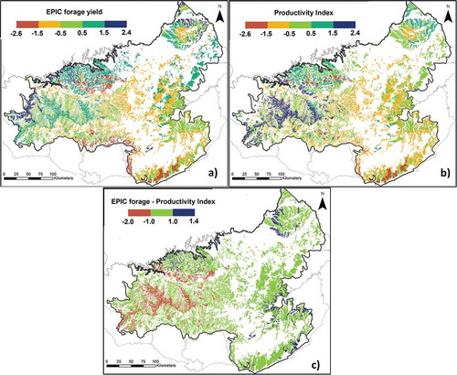
Figure 4. Graphical comparison between standardized values of simulated EPIC grassland production averaged over 15 years and the CONEAT productivity index (PI) grouped in each of the representative CONEAT units (Points). Dotted line is the linear regression

Cropland ecosystem

We selected the soybean crop (Section 2.3.2.2) to test the behavior of the spatial version for the cropland ecosystem. We compared the Geospatial-EPIC-UY annual soybean grain yield outputs for the whole region against the national soybean grain yearly averages during the period 2000–2015 (MGAP-DIEA, 2016b). First, there was a good agreement between modeled annual crop yields and the country yield averages (R² = 0.56, p < 0.05; Figure 5a). A t-test revealed no statistically significant differences (p < 0.05) between the two means (y_sim = 2.36 Mg ha⁻¹, y_obs = 2.01 Mg ha⁻¹, and Std Err = 0.20). Second, we analyzed the inter-annual behavior (Figure 5b) and found that the model captures well the inter-annual variation in crop yields. The main exception occurred in 2010 when the model overestimated production, an exception likely related to wet conditions in this summer and fall (INIA Uruguay – GRAS Unit, 2016) which may have reduced the efficiency of crop harvest operations.

Figure 5. Graphical comparison between EPIC modeled annual soybean grain yield (15 years) and national statistics (MGAP-DIEA, 2016b) (a) correlation considering all years and (b) the time-series

3.2 Potential carbon fluxes changes

After developing and validating Geospatial-EPIC-UY, we analyzed the likely impact of hypothetical land use changes on ecosystem carbon fluxes (NEE, RSPC, NPP) when the entire potentially cultivable area was converted from grassland to cropland, considering soybean monoculture as the option most likely to cause the most negative impact on the environment (Figure 6).

Figure 6. Maps of EPIC simulations over a period of 15 years (1996–2015) of average yearly carbon fluxes of net primary productivity (NPP), heterotrophic soil respiration (RSPC) and net ecosystem exchange (NEE) of Grassland, Cropland and Grassland minus Cropland

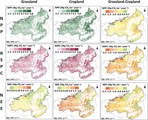
The modeled results showed that during the study period, averaging across the region, the NEE of the grassland was 0.10 and the cropland was 0.70 Mg CO₂ ha⁻¹ year⁻¹. Thus, both ecosystems emitted CO₂ to the atmosphere or acted as a soil C source; however, while the grassland was close to being C neutral, the cropland emitted a considerable amount. Furthermore, the grassland NEE was less variable than the cropland (Figs. 6 and 7). The difference in NEE between the grassland and cropland was caused mainly by the difference in RSPC (grassland = 3.60, cropland = 4.49 Mg CO₂ ha⁻¹ year⁻¹) rather than NPP (grassland = 3.50, cropland = 3.79 Mg CO₂ ha⁻¹ year⁻¹).

Figure 7. Simulated carbon fluxes (NPP, RSPC, NEE) on grassland and cropland by soils crop’s suitable class. For each class, boxes are delimiting the 25 and 75 percentile with the median inside, ‘X’ are the mean of simulated variables by class, whiskers are 10 and 90 percentile

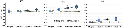
In addition to differences in average carbon budgets, there was high spatial variability, particularly in cropland (Figure 6). Comparing the map of modeled cropland results with the map of soil suitability classes (Fig. S10), we found higher NEE in the more suitable classes and lower for the marginal class. By classifying the data by soil suitability (Figure 7), low variability was observed within and between the grassland classes. However, on cropland, NPP was higher on more suitable classes, characterized by soils with better conditions (fertility and drainage) to grow crops, A similar trend was also observed for RSPC, but with larger differences, and consequently, the NEE increased with soil suitability.

4 Discussion

Here, we developed a geospatial tool (Geospatial-EPIC-UY) integrating the biophysical model EPIC with local climate, land, and management data to quantify the impact of land use conversions taking place in South-Center Uruguay on short- and long-term ecosystem productivity, soil quality and carbon fluxes at field and regional scales.

At a field scale, after the adaptation, calibration, and validation steps, EPIC successfully represented the natural grassland ecosystem of the study region. Our results capture the mean response of historic yearly forage yields and the inter-annual variability (dry-wet years). In the seasonal representation, as expected since summer grass was used as the base, the model slightly overpredicted in the summer and underpredicted in the winter. This underprediction in the winter had almost no impact in our results due to the reported low production in the winter (~0.40 Mg ha⁻¹) (Berretta, 2003). Given that forage yield was the main yearly C input, this low production in the winter was counterbalanced with the summer forage production. The model adjustment of the forage yield (difference, standard error, and correlation) is similar to those reported for other cropping conditions (Apezteguía et al., 2009; Causarano et al., 2008) where EPIC had been calibrated given the lack of published calibrations in natural grassland environments. Finally, the model captured the negative trends of measured soil C, and simulated values also agree with those reported by Piñeiro et al. (2006) for the Pampa grasslands.

For the cropland at a field scale, after automatic calibration and validation with the data of the two sites, we achieved an acceptable representation of the yield production of the modeled crops. This agreement of simulated and measured results is similar to previous EPIC calibration exercises (Apezteguía et al., 2009). Finally, the model captured well the trends in soil carbon loss. The higher soil carbon loss simulated in cropland than in grassland, even under no-tillage, agrees with previous research of grassland conversion to cropland (Culman et al., 2010; DuPont et al., 2010).

After developing the Geospatial-EPIC-UY, the validation showed that at regional scale, the grassland forage production variation over the region was well represented by the model, and also, the yearly modeled values of the whole region over this period agree with those of Ayala and Bermudez (2005), Bermudez and Ayala (2005), and Formoso (2005). In addition, a good representation was achieved in the cropland ecosystem when compared with national statistics (MGAP-DIEA, 2016b).

After the successful validation, we addressed the likely impact of hypothetical land use changes from grassland to cropland (soybean monoculture) on ecosystem carbon fluxes. The grassland land cover was permanent pasture present since the introduction of domestic herbivores (cattle, sheep, and horses) by European settlers in the XVI century. Livestock densities increased since then and reached a stable stocking rate by the 1900s, when all land was fenced, and remained mostly unchanged till now (Fig. S12), consuming between 30% and 60% of annual NPP (MGAP-DIEA, 2016a; Soriano et al., 1992). This stocking rate equilibrium is reflected in the average grassland carbon fluxes. On average, for the whole region and the study period, C emissions (NEE) from grasslands were close to neutral (0.1 Mg CO₂ ha⁻¹ year⁻¹) with low variability across the region (Figures 6 and 7), and this NEE was the result of almost a balance between the annual productivity (NPP) and heterotrophic respiration (RSPC). These rather small C emissions agree with the small simulated soil C loss and small long-term C losses reported by Piñeiro et al. (2006) for the Rio de la Plata region. Rolinski et al. (2018) reported results of a dynamic global vegetation model (LJmL) showing no changes in soil C stocks in temperate regions (including our study region) under continuous grazing and with similar stocking rates.

Conversion to cropland produced a significant alteration of the C cycle across the study region. On average, net cropland C emissions (NEE) contributed seven times more C to the atmosphere (and showed larger variability) than emissions from grassland (Figs.6 and 7). A similar trend of C loss was reported by Abraha et al. (2018) in the US where converting grasslands to croplands (no-till corn with partial residue removal) resulted in a continued net C loss to the atmosphere. This higher NEE on cropland arose from the positive difference between heterotrophic respiration and crop NPP. In this region, the temperature and hydrologic regime favor a rapid turnover of soil organic matter, which is roughly 1.5 times faster than cooler and wetter conditions (US. Midwest) and 5 times faster than cooler and drier regions (US Oregon) (S. S. Mazzilli et al., 2012). Further, under these conditions, the decomposition of soybean residues is quick because of the quick turnover of the soybean crop residues after harvesting (Alvarez et al., 1998). Ernst et al. (2002) found that the stubble was barely visible 4 months after harvest. Consequently, the C input from soybean residues, under these environmental conditions, is low as reported by S. R. Mazzilli et al. (2015) who found soybean residue contribution to the soil organic carbon pool to be 0.4% and 1.4% of the NPP from aboveground and belowground residues, respectively.

In addition to differences in average C budgets over the region, our analysis of the spatial distribution of the different components of the C fluxes over the region revealed a high spatial variability across the study region, particularly in cropland (Figure 6). After classifying the HSMUs by soil crop suitability, we found a large difference in the RSPC among groups, where the RSPC increased with the increase in crop suitability. The more suitable soils have higher natural SOC than the less suitable, so the main driver is attributable to the higher C oxidation from soils with higher SOC stocks. The result is that the NEE increased with soil suitability. These results confirm that land use conversions that cause soil and vegetation disturbances will result in a large net C emission to the atmosphere as was previously reported for other regions (Fargione et al., 2008; Gelfand et al., 2011).

These results highlight the potential risk of an extended land use conversion in the C cycle, changing an almost neutral C system (grassland) to C source (cropland). This could be ameliorated if, before the conversion, mitigation strategies considering the different soil crop suitability are adopted across the different spatial scales (region, farm, and parcel). At a region scale, we conducted a hypothetical conversion of all the areas, but as could be observed in Figure 1, in 2010, vast part of the west region has already been converted to cropland, so regionally, the land use change policies need to focus on the areas that still are not transformed (center-east) and have higher risk of increased C losses (Figure 6 Grass-Crop NEE yellow to orange areas). At a farm scale, based on detailed soil maps, the identification by farmers of areas with different soil crop capabilities, defining new parcel if necessary and planning the use for each parcel based on suitability. Finally, at a parcel level, the adoption of best management practice strategies adapted to the region could be recommended. These options could range from ones that could produce less or more impacts on current production systems: a) inclusion of winter cover crops (oat and rye grass) in the rotation after soybean, diminishing the decomposition of the residues of soybean and increasing the input of biomass (Varela et al., 2014), b) adopting a crop rotation with higher C return to soils and cover during the year with the inclusion of wheat and sorghum (Pravia et al., 2019; Terra et al., 2006) and c) even better, by adopting a crop/grass rotation that was deemed as a proved long-term suitable management option (Díaz Rossello, 1992). Even though it was beyond the scope of the present research, we conducted an analysis of the impact of the first two options considering different soil capabilities in one site that confirm the benefits of these potential strategies (Appendix 4, Supplemental Data).

Furthermore, although the current grassland management was close to C neutral, it may be improved by grazing management and stocking rate adjustments. In grassland ecosystems, grazing by livestock plays an important role in regulating the stock and dynamics of C. Our approach when modeling this ecosystem includes the grazing processes assuming a well-managed grassland with fixed stocking rate that covers the animal nutrient requirements on a yearly basis. However, pastures in the study region, under continuous grazing year around, are subject to cycles of overgrazing and undergrazing, and these processes occur across temporal and spatial scales. Temporarily, the almost fixed stocking rate grazing a pasture with significant seasonal variation in the NPP generates period of excess and deficit across the year, this condition is exacerbated in drier years, spatially within the parcels (patchiness) resulting from difference in livestock grazing distribution based on the animals’ grazing preferences and among parcels/farms as a consequence of differences in livestock density (Natural Grassland Working Group, 2017). Overgrazing occurs when forage production does not cover the livestock nutritional requirements, and it is the most significant negative process in the study area producing loss of plant species, rise of weed population, increase in soil erosion and finally decrease in NPP and belowground biomass, a primary control of soil organic C formation (Picasso et al., 2014; Zhu et al., 2018). On the contrary, undergrazing occurs when forage available exceeds livestock demands, produces in the medium term a decline in the forage quality, promotes shrub encroachment, and, as a consequence, decreases NPP and belowground biomass (López-Mársico et al., 2015). We did not include these processes in our simulations because the diverse spatial and temporal distribution remains a topic of future study requiring, currently unavailable, new field data and mapping of the affected areas.

These results showed that this modeling approach is a valuable tool to address the changes in the C balance caused by conversion of grassland to cropland, which could help in the development of land use policies by government or public agencies, considering also potential mitigation options based on new, more sustainable, methods of crop production. Moreover, it was also shown that it can be applied to large areas, in addition to a field scale, under contemporary grassland-cropland conversions and future climate, land use, and management scenarios. One of the limitations with this research was the scarcity of field data required to perform the calibration/validation steps in modeling. This deficiency suggests a need to conduct more field measurements using conventional agronomic, soil and weather techniques as well as new types of monitoring of relevant gas fluxes (e.g. eddy covariance measurements of NEE) or the inclusion of satellite observations (e.g. weather and NPP) that are currently available worldwide.

Disclosure of potential conflicts of interest

No potential conflict of interest was reported by the author(s).

Acknowledgments

We would like to thank the following individuals and institutions for their assistance: José Terra, Walter Ayala and Andrés Quincke (INIA, Uruguay); Daniel Formoso (SUL, Uruguay), Mario Bidegain (INUMET, Uruguay); Taras Lychuk, Varaprasad Bandaru, Curtis Jones, Matthew Hansen, George Hurtt, and Adel Shirmohammadi (University of Maryland, USA); and Jimmy Williams (Texas A&M University, USA).

Supplementary material

Supplemental data for this article can be accessed here.

Additional information

Funding

This work was supported by the National Agricultural Research Institute (INIA) of Uruguay, by a fellowship of the Department of Geographical Sciences, University of Maryland, College Park, MD to the senior author, and by the NASA Harvest Program (Grant No. NNX16AP16G).

References

- Abraha, M., Hamilton, S.K., Chen, J., & Robertson, G.P. (2018). Ecosystem carbon exchange on conversion of Conservation Reserve Program grasslands to annual and perennial cropping systems. Agricultural and Forest Meteorology, 253–254(October 2017), 151–160. https://doi.org/10.1016/j.agrformet.2018.02.016
- Adejuwon, J. (2005). Assessing the suitability of the EPIC crop model for use in the study of impacts of climate variability and climate change in West Africa. Singapore Journal of Tropical Geography, 26(1), 44–60. https://doi.org/10.1111/j.0129-7619.2005.00203.x
- Altesor, A., Piñeiro, G., Lezama, F., Jackson, R.B., Sarasola, M., & Paruelo, J.M. (2006). Ecosystem changes associated with grazing in subhumid South American grasslands. Journal of Vegetation Science, 17(3), 323–332. Blackwell Publishing Ltd. https://doi.org/10.1111/j.1654-1103.2006.tb02452.x
- Alvarez, R., Russo, M.E., Prystupa, P., Scheiner, J.D., & Blotta, L. (1998). Soil Carbon Pools under Conventional and No-Tillage Systems in the Argentine Rolling Pampa. Agronomy Journal, 90(2), 138. https://doi.org/10.2134/agronj1998.00021962009000020003x
- Apezteguía, H., Izaurralde, R.C., & Sereno, R. (2009). Simulation study of soil organic matter dynamics as affected by land use and agricultural practices in semiarid Córdoba, Argentina. Soil and Tillage Research, 102(1), 101–108. https://doi.org/10.1016/j.still.2008.07.016
- AUSID. (2009). Annual conference and field day 2009 - La Manera. https://ausid.com.uy/jornada2009.html
- AUSID. (2010). Annual conference and field day 2010 - Las Brisas. AUSID. https://ausid.com.uy/jornada2010a.html
- Ayala, W., & Bermudez, R. (2005). Estrategias de manejo en campos naturales sobre suelos de lomadas en la región Este. Seminario De Actualización Técnica En Manejo De Campo Natural, (pp. 41–50). INIA Uruguay..
- Baethgen, W.E. (2003). Utilización del modelo Century para estudiar la dinámica de carbono y nitrógeno [Using the Century model to study the dynamics of carbon and nitrogen]. In R. Gomez & M. Albicette (Eds.). 40 años de rotaciones agrícolas-ganaderas (40 years of agricultural-livestock rotations) (pp. 9–18). National Agricultural Research Institute.
- Baeza, S., & Paruelo, J.M. (2020). Land Use/Land Cover Change (2000–2014) in the Rio de la Plata Grasslands: An analysis based on MODIS NDVI time series. Remote Sensing, 12(3), 381. https://doi.org/10.3390/rs12030381
- Balkovič, J., van der Velde, M., Schmid, E., Skalský, R., Khabarov, N., Obersteiner, M., Stürmer, B., & Xiong, W. (2013). Pan-European crop modelling with EPIC: Implementation, up-scaling and regional crop yield validation. Agricultural Systems, 120, 61–75. https://doi.org/10.1016/j.agsy.2013.05.008
- Bermudez, R., & Ayala, W. (2005). Producción de forraje de un campo natural de la zona de Lomadas del Este [Forage production of a natural grassland field of the hilly Eastern]. Seminario De Actualización Técnica En Manejo De Campo Natural, 33–39. INIA Uruguay.
- Bernardos, J.N., Viglizzo, E.F., Jouvet, V., Lértora, F.A., Pordomingo, A.J., & Cid, F.D. (2001). The use of EPIC model to study the agroecological change during 93 years of farming transformation in the Argentine pampas. Agricultural Systems, 69(3), 215–234. https://doi.org/10.1016/S0308-521X(01)00027-0
- Berretta, E.J. (2003). Uruguay in Country Pasture Profiles. Food and Agriculture Organization (FAO). http://www.fao.org/ag/AGP/AGPC/doc/Counprof/uruguay/uruguay.htm
- Billen, N., Röder, C., Gaiser, T., & Stahr, K. (2009). Carbon sequestration in soils of SW-Germany as affected by agricultural management—Calibration of the EPIC model for regional simulations. Ecological Modelling, 220(1), 71–80. https://doi.org/10.1016/j.ecolmodel.2008.08.015
- Capurro Etchegaray, M. (1977). CONEAT, reseña de la metodología adoptada para determinar la productividad a nivel predial [National Commission for the Agronomic Study of Soils (CONEAT), a review of the methodology adopted to determine productivity at the farm level]. Fundación de la Cultura Universitaria.
- Caride, C., Piñeiro, G., & Paruelo, J.M. (2012). How does agricultural management modify ecosystem services in the argentine Pampas? The effects on soil C dynamics. Agriculture, Ecosystems & Environment, 154, 23–33. https://doi.org/10.1016/j.agee.2011.05.031
- Castaño-Sánchez, J.P., Gimenez, A., Ceroni, M., Furest, J., Aunchayna, R., & Bidegain, M. (2011). Caracterización Agroclimática del Uruguay (1980–1989) [Agroclimatic characterization of Uruguay (1980–2009)] (Issue 193). INIA Uruguay.
- Castro, M., Coutiño, M.J., & Perez, O. (2015). Evaluación de cultivares de cultivos de verano e invierno INIA La Estanzuela y Young (2000–2014) [Winter and Summer Field Crop Variety Trials]. INIA Uruguay. http://www.inia.org.uy/convenio_inase_inia/resultados/index_00.htm
- Causarano, H.J., Doraiswamy, P.C., McCarty, G.W., Hatfield, J.L., Milak, S., & Stern, A.J. (2008). EPIC modeling of soil organic carbon sequestration in croplands of Iowa. Journal of Environmental Quality, 37(4), 1345–1353. https://doi.org/10.2134/jeq2007.0277
- Causarano, H.J., Doraiswamy, P.C., Muratova, N., Pachikin, K., McCarty, G.W., Akhmedov, B., & Williams, J.R. (2011). Improved modeling of soil organic carbon in a semiarid region of Central East Kazakhstan using EPIC. Agronomy for Sustainable Development, 31(2), 275–286. https://doi.org/10.1051/agro/2010028
- Causarano, H.J., Shaw, J.N., Franzluebbers, A.J., Reeves, D.W., Raper, R.L., Balkcom, K.S., Norfleet, M.L., & Izaurralde, R.C. (2007). Simulating field-scale soil organic carbon dynamics using EPIC. Soil Science Society of America Journal, 71(4), 1174–1185. https://doi.org/10.2136/sssaj2006.0356
- Chapin, F.S., Woodwell, G.M., Randerson, J.T., Rastetter, E.B., Lovett, G.M., Baldocchi, D.D., Clark, D.A., Harmon, M.E., Schimel, D.S., Valentini, R., Wirth, C., Aber, J.D., Cole, J.J., Goulden, M.L., Harden, J.W., Heimann, M., Howarth, R.W., Matson, P.A., McGuire, A.D., & Schulze, E.-D. (2006). Reconciling Carbon-cycle Concepts, Terminology, and Methods. Ecosystems, 9(7), 1041–1050. https://doi.org/10.1007/s10021-005-0105-7
- Coupland, R.T. (1992). Overview of South American Grasslands. In R.T. Coupland (Ed.), Ecosystems of the world (Issue 18, pp. 363–366). Elsevier.
- Culman, S.W., DuPont, S.T., Glover, J.D., Buckley, D.H., Fick, G.W., Ferris, H., & Crews, T.E. (2010). Long-term impacts of high-input annual cropping and unfertilized perennial grass production on soil properties and belowground food webs in Kansas, USA. Agriculture, Ecosystems & Environment, 137(1–2), 13–24. https://doi.org/10.1016/j.agee.2009.11.008
- Díaz Rossello, R. (1992). Evolución de la materia orgánica en rotaciones de cultivos con pasturas. Revista INIA De Investigaciones Agronómicas, 1(1), 103–110.
- DuPont, S.T., Culman, S.W., Ferris, H., Buckley, D.H., & Glover, J.D. (2010). No-tillage conversion of harvested perennial grassland to annual cropland reduces root biomass, decreases active carbon stocks, and impacts soil biota. Agriculture, Ecosystems & Environment, 137(1–2), 25–32. https://doi.org/10.1016/j.agee.2009.12.021
- Ernst, O., Bentancur, O., & Borges, R. (2002). Decomposition of Crop Residues Under No-Till Management : Wheat, Corn, Soybeans and Wheat. Agrociencia, 6, 20–26.
- EUROSTAT. (2013). Eurostat Statistics Explained. Glossary: Livestock Unit (LSU]. https://ec.europa.eu/eurostat/statistics-explained/index.php/Glossary:Livestock_unit_(LSU)
- Fargione, J., Hill, J., Tilman, D., Polasky, S., & Hawthorne, P. (2008). Land clearing and the biofuel carbon debt. Science, 319(5867), 1235–1238. https://doi.org/10.1126/science.1152747
- Farina, R., Seddaiu, G., Orsini, R., Steglich, E., Roggero, P.P., & Francaviglia, R. (2011). Soil carbon dynamics and crop productivity as influenced by climate change in a rainfed cereal system under contrasting tillage using EPIC. Soil and Tillage Research, 112(1), 36–46. https://doi.org/10.1016/j.still.2010.11.002
- Formoso, D. (2005). La investigación en utilización de pasturas naturales sobre cristalino desarrollada por el SUL [Reseach in natural pastures over granite soils made by SUL]. In Seminario de actualización Técnica en manejo de campo natural (pp. 51–59). INIA Uruguay.
- Freier, K.P., Schneider, U.A., & Finckh, M. (2011). Dynamic interactions between vegetation and land use in semi-arid Morocco: Using a Markov process for modeling rangelands under climate change. Agriculture, Ecosystems & Environment, 140(3–4), 462–472. https://doi.org/10.1016/j.agee.2011.01.011
- Gaiser, T., de Barros, I., Sereke, F., & Lange, F.-M. (2010). Validation and reliability of the EPIC model to simulate maize production in small-holder farming systems in tropical sub-humid West Africa and semi-arid Brazil. Agriculture, Ecosystems & Environment, 135(4), 318–327. https://doi.org/10.1016/j.agee.2009.10.014
- Gassman, P.W., Williams, J.R., Benson, V., Izaurralde, R.C., Hauck, L.M., Jones, C.A., Atwood, J.D., Kiniry, J.R., & Flowers, J.D. (2005). Historical development and applications of the EPIC and APEX models. In Director. Center for Agricultural and Rural Development, Iowa State University. https://doi.org/10.13031/2013.17074.
- Gelfand, I., Zenone, T., Jasrotia, P., Chen, J., Hamilton, S.K., & Robertson, G.P. (2011). Carbon debt of Conservation Reserve Program (CRP) grasslands converted to bioenergy production. Proceedings of the National Academy of Sciences of the United States of America, 108(33), 13864–13869. https://doi.org/10.1073/pnas.1017277108
- Guerschman, J.P., Paruelo, J.M., Di Bella, C.M., Giallorenzi, M.C., & Pacin, F. (2003). Land cover classification in the Argentine Pampas using multi-temporal Landsat TM data. International Journal of Remote Sensing, 24(17), 3381–3402. https://doi.org/10.1080/0143116021000021288
- Houghton, R.A. (2018). Interactions Between Land-Use Change and Climate-Carbon Cycle Feedbacks. In Current Climate Change Reports (Vol. 4(2), 115–127). Springer. https://doi.org/10.1007/s40641-018-0099-9.
- Houghton, R.A., & Nassikas, A.A. (2017). Global and regional fluxes of carbon from land use and land cover change 1850–2015. Global Biogeochemical Cycles, 31(3), 456–472. https://doi.org/10.1002/2016GB005546
- INIA Uruguay - GRAS Unit. (2016). INIA - Mapas de precipitación acumulada [INIA accumulated precipitation maps]. http://www.inia.uy/investigación-e-innovación/unidades/GRAS/Clima/Precipitación-nacional/Mapas-de-precipitación-acumulada
- IPCC. (2003). Good Practice Guidance for Land Use, Land-Use Change and Forestry - Methodology Report.
- Izaurralde, R.C., McGill, W.B., & Williams, J.R. (2012). Development and application of the EPIC model for carbon cycle, greenhouse-gas mitigation, and biofuel studies. In M. A. Liebig, A. J. Franzluebbers, & R. F. Follet (Eds.), Managing agricultural greenhouse gases: Coordinated agricultural research through GRACEnet to address our changing climate (Issue 17, pp. 293–308). Academic Press. http://site.ebrary.com/lib/umd/docDetail.action?docID=10566556
- Izaurralde, R.C., Williams, J.R., McGill, W.B., Rosenberg, N.J., & Jakas, M.C.Q. (2006). Simulating soil C dynamics with EPIC: Model description and testing against long-term data. In Ecological Modelling (Vol. 192, Issues 3–4, pp. 362–384). https://doi.org/10.1016/j.ecolmodel.2005.07.010.
- Izaurralde, R.C., Williams, J.R., Post, W.M., Thomson, A.M., McGill, W.B., Owens, L.B., & Lal, R. (2007). Long-term modeling of soil C erosion and sequestration at the small watershed scale. In Climatic Change (Vol. 80, Issues 1–2, pp. 73–90). Springer Netherlands. https://doi.org/10.1007/s10584-006-9167-6.
- Lal, R. (2002). Soil carbon dynamics in cropland and rangeland. Environmental Pollution, 116(3), 353–362. https://doi.org/10.1016/S0269-7491(01)00211-1
- Lanfranco Crespo, B., & Sapriza Fraga, G. (2011). El índice CONEAT como medida de productividad y valor de la tierra [The CONEAT index as a measure of land productivity and value]. (INIA Uruguay (ed.); Serie Técn). INIA Uruguay.
- López-Mársico, L., Altesor, A., Oyarzabal, M., Baldassini, P., & Paruelo, J.M. (2015). Grazing increases below-ground biomass and net primary production in a temperate grassland. Plant and Soil, 392(1–2), 155–162. https://doi.org/10.1007/s11104-015-2452-2
- Ma, K., Liu, J., Balkovič, J., Skalský, R., Azevedo, L.B., & Kraxner, F. (2016). Changes in soil organic carbon stocks of wetlands on China’s Zoige plateau from 1980 to 2010. Ecological Modelling, 327, 18–28. https://doi.org/10.1016/j.ecolmodel.2016.01.009
- Mazzilli, S., Piñeiro, G., & Kemanian, A. (2012). Priming effects on soil organic carbon decomposition induced by high C:N crop inputs. Agrociencia Uruguay, 16(3), 191–198. https://doi.org/10.31285/AGRO.16.669
- Mazzilli, S.R., Kemanian, A.R., Ernst, O.R., Jackson, R.B., & Piñeiro, G. (2015). Greater humification of belowground than aboveground biomass carbon into particulate soil organic matter in no-till corn and soybean crops. Soil Biology and Biochemistry, 85(September 2016), 22–30. https://doi.org/10.1016/j.soilbio.2015.02.014
- MGAP Uruguay, MVOTMA Uruguay, & FAO. (2011). Mapa de Cobertura del Suelo de Uruguay - Land Cover Classification System. FAO Uruguay.
- MGAP-DGRNR-CONEAT. (1994). Indice de Productividad grupos de suelos CONEAT (Productivity Index of CONEAT Soil map).
- MGAP-DIEA. (2015). Anuario estadístico Agropecuario 2015 [Agricultural Statistical Yearbook 2015]. MGAP.
- MGAP-DIEA. (2016a). Anuario estadístico Agropecuario 2016 [Agricultural Statistical Yearbook 2016]. MGAP.
- MGAP-DIEA. (2016b). Series Historicas de Estadísticas Agropecuarias [Historical Series of Agricultural Statistics]. MGAP Uruguayhttp://www.mgap.gub.uy/portal/page.aspx?2,diea,diea-series-historicas,O,es,0
- MGAP-RENARE-DSA. (2003). Zonificación de cultivos de verano de secano [Zoning rainfed summer crops]. MGAP Uruguay.
- Natural Grassland Working Group. (2017). Producción animal sostenible en pastoreo sobre campo natural [Sustainable livestock production grazing natural grasslands]. MGAP. http://www.mgap.gub.uy/sites/default/files/multimedia/libro_campo_natural_final_en_baja.pdf
- Parton, W.J., Stewart, J.W.B., & Cole, C.V. (1988). Dynamics of C, N, P and S in grassland soils: A model. Biogeochemistry, 5(1), 109–131. https://doi.org/10.1007/BF02180320
- Picasso, V.D., Modernel, P.D., Becoña, G., Salvo, L., Gutiérrez, L., & Astigarraga, L. (2014). Sustainability of meat production beyond carbon footprint: A synthesis of case studies from grazing systems in Uruguay. Meat Science, 98(3), 346–354. https://doi.org/10.1016/j.meatsci.2014.07.005
- Piñeiro, G., Paruelo, J.M., & Oesterheld, M. (2006). Potential long-term impacts of livestock introduction on carbon and nitrogen cycling in grasslands of Southern South America. Global Change Biology, 12(7), 1267–1284. https://doi.org/10.1111/j.1365-2486.2006.01173.x
- Pravia, M.V., Kemanian, A.R., Terra, J.A., Shi, Y., Macedo, I., & Goslee, S. (2019). Soil carbon saturation, productivity, and carbon and nitrogen cycling in crop-pasture rotations. Agricultural Systems, 171, 13–22. https://doi.org/10.1016/j.agsy.2018.11.001
- R Development Core Team. (2013). R Software. R: A Language and Environment for Statistical Computing. R Foundation for Statistical Computing, Vienna, Austria. https://www.R-project.org/
- Rahman, M.R., Shi, Z.H., & Chongfa, C. (2009). Soil erosion hazard evaluation—An integrated use of remote sensing, GIS and statistical approaches with biophysical parameters towards management strategies. Ecological Modelling, 220(13–14), 1724–1734. https://doi.org/10.1016/j.ecolmodel.2009.04.004
- Rolinski, S., Müller, C., Heinke, J., Weindl, I., Biewald, A., Leon Bodirsky, B., Bondeau, A., Boons-Prins, E.R., Bouwman, A.F., Leffelaar, P.A., Roller, J.A.T., Schaphoff, S., & Thonicke, K. (2018). Modeling vegetation and carbon dynamics of managed grasslands at the global scale with LPJmL 3.6. Geoscientific Model Development, 11(1), 429–451. https://doi.org/10.5194/gmd-11-429-2018
- Roloff, G., De Jong, R., Zentner, R.P., Campbell, C.A., & Benson, V.W. (1998). Estimating spring wheat yield variability with EPIC. Canadian Journal of Soil Science, 78(3), 541–549. https://doi.org/10.4141/S97-063
- Sala, O.E., Lauenroth, W.K., & Burke, I.C. (1996). Carbon Budgets of Temperate Grasslands and the Effects of Global Change. In A.I. Breymeyer, D.O. Hall, J.M. Melillo, & G.I. Agren (Eds.), Global Change: Effects on Coniferous Forests and Grasslands (56thed., xxiv + 459 pp.). John Wiley. http://www.scopenvironment.org/downloadpubs/scope56/Chapter05.html%5Cnhttp://www.scopenvironment.org/downloadpubs/scope56/contents.html
- Schwalm, C.R., Williams, C.A., Schaefer, K., Anderson, R., Arain, M.A., Baker, I., Barr, A., Black, T.A., Chen, G., Chen, J.M., Ciais, P., Davis, K.J., Desai, A., Dietze, M., Dragoni, D., Fischer, M.L., Flanagan, L.B., Grant, R., Gu, L., & Verma, S.B. (2010). A model-data intercomparison of CO 2 exchange across North America: Results from the North American Carbon Program site synthesis. Journal of Geophysical Research, 115(4), G00H05. https://doi.org/10.1029/2009JG001229
- Sharda, V., Mekonnen, M.M., Ray, C., & Gowda, P.H. (2020). Use of Multiple Environment Variety Trials Data to Simulate Maize Yields in the Ogallala Aquifer Region: A Two Model Approach. Journal of the American Water Resources Association, 57(2), 1–15. https://doi.org/10.1111/1752-1688.12873
- Smith, P., Davies, C.A., Ogle, S., Zanchi, G., Bellarby, J., Bird, N., Boddey, R.M., McNamara, N.P., Powlson, D., Cowie, A., Noordwijk, M., Davis, S.C., Richter, D.D.B., Kryzanowski, L., Wijk, M.T., Stuart, J., Kirton, A., Eggar, D., Newton-Cross, G., & Braimoh, A.K. (2012). Towards an integrated global framework to assess the impacts of land use and management change on soil carbon: Current capability and future vision. Global Change Biology, 18(7), 2089–2101. https://doi.org/10.1111/j.1365-2486.2012.02689.x
- Sohl, T.L., Sleeter, B.M., Zhu, Z., Sayler, K.L., Bennett, S., Bouchard, M., Reker, R., Hawbaker, T., Wein, A., Liu, S., Kanengieter, R., & Acevedo, W. (2012). A land-use and land-cover modeling strategy to support a national assessment of carbon stocks and fluxes. Applied Geography34, 111–124). https://doi.org/10.1016/j.apgeog.2011.10.019.
- Soriano, A., León, R.J.C., Sala, O.E., Lavado, R.S., Deregibus, V.A., Cahuépé, M.A., Scaglia, O.A., Velázquez, C.A., & Lemcoff, J.H. (1992). Río de la Plata Grasslands. In R.T. Coupland (Ed.), Ecosystems of the world (Issue 19, pp. 367–407). Elsevier. http://cat.inist.fr/?aModele=afficheN&cpsidt=5613792
- Soriano, A., & Paruelo, J.M. (1992). Biozones: Vegetation Units Defined by Functional Characters Identifiable with the Aid of Satellite Sensor Images. Global Ecology and Biogeography Letters, 2(3), 82. https://doi.org/10.2307/2997510
- Terra, J.A., García Préchac, F., Salvo, L., & Hernández, J. (2006). Soil use intensity impacts on total and particulate soil organic Matter in no-till crop-pasture rotations under direct grazing. Advances in Geoecology, 38, 233–241.
- Tiemeyer, B., Freibauer, A., Borraz, E.A., Augustin, J., Bechtold, M., Beetz, S., Beyer, C., Ebli, M., Eickenscheidt, T., Fiedler, S., Förster, C., Gensior, A., Giebels, M., Glatzel, S., Heinichen, J., Hoffmann, M., Höper, H., Jurasinski, G., Laggner, A., & Drösler, M. (2020). A new methodology for organic soils in national greenhouse gas inventories: Data synthesis, derivation and application. Ecological Indicators, 109(October 2019), 105838. https://doi.org/10.1016/j.ecolind.2019.105838
- Varela, M.F., Scianca, C.M., Taboada, M.A., & Rubio, G. (2014). Cover crop effects on soybean residue decomposition and P release in no-tillage systems of Argentina. Soil and Tillage Research, 143(November 2014), 59–66. https://doi.org/10.1016/j.still.2014.05.005https://doi.org/10.1016/j.still.2014.05.005.
- Vega, E., Baldi, G., Jobbágy, E.G. & Paruelo, J.M. (2009). Land use change patterns in the Río de la Plata grasslands: The influence of phytogeographic and political boundaries. In Agriculture, Ecosystems and Environment 134(3–4), 287–292. https://doi.org/10.1016/j.agee.2009.07.011.
- West, T.O., Bandaru, V., Brandt, C.C., Schuh, A.E., & Ogle, S.M. (2011). Regional uptake and release of crop carbon in the United States. Biogeosciences, 8(8), 2037–2046. https://doi.org/10.5194/bg-8-2037-2011
- Williams, J.R., Arnold, J.G., Kiniry, J.R., Gassman, P.W., & Green, C.H. (2008). History of model development at Temple, Texas. In Hydrological Sciences Journal - Journal Des Sciences Hydrologiques 53(5), 948–960. https://doi.org/10.1623/hysj.53.5.948.
- Williams, J.R., Jones, C.A., & Dyke, P.T. (1984). A modelling approach to determining the relationship between erosion and soil productivity. Transactions - American Society of Agricultural Engineers, 27(1), 129–144. https://doi.org/10.13031/2013.32748
- Williams, J.R., Wang, E., Meinardus, A., Harman, W.L., Siemers, M., & Atwood, J.D. (2006). EPIC user guide v.0509. Texas A&M AgriLife Extension Center.
- Zambrano-Bigiarini, M., & Rojas, R. (2013). A model-independent Particle Swarm Optimisation software for model calibration. Environmental Modelling and Software, 43, 5–25. https://doi.org/10.1016/j.envsoft.2013.01.004
- Zhang, X., Izaurralde, R.C., Manowitz, D., West, T.O., Post, W.M., Thomson, A.M., Bandaru, V.P., Nichols, J., & Williams, J.R. (2010). An integrative modeling framework to evaluate the productivity and sustainability of biofuel crop production systems. GCB Bioenergy, 2(5), 258–277. https://doi.org/10.1111/j.1757-1707.2010.01046.x
- Zhang, X., Izaurralde, R.C., Manowitz, D.H., Sahajpal, R., West, T.O., Thomson, A.M., Xu, M., Zhao, K., LeDuc, S.D., & Williams, J.R. (2015). Regional scale cropland carbon budgets: Evaluating a geospatial agricultural modeling system using inventory data. Environmental Modelling & Software, 63, 199–216. https://doi.org/10.1016/j.envsoft.2014.10.005
- Zhu, G., Tang, Z., Chen, L., Shangguan, Z., & Deng, L. (2018). Overgrazing depresses soil carbon stock through changing plant diversity in temperate grassland of the loess plateau. Plant, Soil and Environment, 64(1), 1–6. https://doi.org/10.17221/610/2017-PSE