Numerical investigation of indoor thermal comfort and air quality for an office equipped with corner impinging jet ventilation

ABSTRACT

This study investigates the feasibility of using only corner impinging jet ventilation (CIJV) for heating and cooling a medium-sized office space with two occupants while maintaining adequate indoor thermal comfort and air quality compared to traditional mixing ventilation systems. This study examines what impact various outdoor temperatures, ranging from −15°C to 25°C, have on an office environment in terms of indoor thermal comfort and air quality. Three different workspace positions were evaluated. The results show that the CIJV system meets the ASHRAE thermal comfort standards for all three positions. In terms of indoor air quality, CIJV performs better than traditional mixing systems, with improved mean age of air and ACE values. This study concludes that CIJV can be used both close and far away from the supply inlets and still provide adequate indoor thermal comfort and air quality during both cooling and heating season.

KEYWORDS:

• corner impinging jet ventilation
• heating and cooling
• computational fluid dynamic
• thermal comfort
• indoor air quality

Nomenclature

ACE	=	air change efficiency [–]
ADS	=	air distribution system
BBR	=	Boverket’s building regulations in Sweden
CFD	=	computational fluid dynamic
CIJV	=	corner impinging jet ventilation
DO	=	discrete ordinates
DR	=	draught rate [%]
DV	=	displacement ventilation
IAQ	=	indoor air quality
IJV	=	impinging jet ventilation
MV	=	mixing ventilation
PMV	=	predicted mean vote
PPD	=	predicted percentage of dissatisfied [%]
RANS	=	Reynolds-averaged Navier–Stokes
RMSE	=	root-mean-square error [%]
ΔT1.1–0.1	=	vertical temperature difference between head and ankle level for a seated person [°C]
H	=	height above floor level [m]
Il	=	local turbulence intensity [%]
$P$	=	pressure [N m−2]
Sct	=	turbulent Schmidt number [m2 s]
Ta	=	local temperature [°C]
$T_o$	=	outdoor air temperature [°C]
$T_s$	=	supply air temperature [°C]
$U_i$	=	mean component of velocity [m s−1]
$U_{in}$	=	nominal air velocity of the inlet device [m s−1]
$k$	=	turbulent kinetic energy [m2 s−2]
$u^{\mathrm{\prime }}$	=	fluctuating component of velocity [m s−1]
$x_i=x,y,z$	=	cartesian spatial coordinates [m]
y+	=	dimensionless wall distance [–]
${\delta }_{ij}$	=	Kronecker delta [–]
ϵ	=	turbulence dissipation rate [m2 s−3]
σt	=	turbulent Prandtl number [–]
$\rho$	=	density [kg m−3]
$-\rho \overline{u_i^{\mathrm{\prime }}}\overline{u_j^{\mathrm{\prime }}}$	=	Reynolds stress tensor [kg m−1 s−2]
${\varphi }_{i,BG}$	=	numerical solution at base grid resolution
${\varphi }_{i,RG}$	=	numerical solution at refined grid resolution
$\mu$	=	dynamic viscosity [kg m−1 s−1]
${\mu }_t$	=	turbulent viscosity [kg m−1 s−1]
$\tau$	=	arithmetic average mean age of air [s]
${\tau }_n$	=	nominal time constant [s]
${\tau }_w$	=	wall shear stress [kg m−1 s−2]
$\nu$	=	kinematic viscosity [m2 s−1]

1. Introduction

The ventilation system is responsible for bringing fresh air into the building while removing stale air and pollutants. A poorly designed or inefficient ventilation system can lead to poor indoor air quality, which can cause health problems for the building’s occupants. In order to accommodate for a good indoor environment in buildings it is important to choose the right ventilation strategy. The type of ventilation system or air distribution system (ADS) used will have a direct impact on the indoor air quality, indoor environment, thermal comfort level as well as energy usage (American Society of Heating and Refrigerating and Air-Conditioning Engineers, 2017; Vimalanathan & Babu, 2014; Yang et al., 2019) in a building. In recent years several alternative air distribution systems have been proposed and researched in order to improve these aspects. One of the early ADS developed is called mixing ventilation (MV). This system is currently dominating the market and has been extensively researched in the past (Ameen et al., 2019b; Cao et al., 2014; Kong et al., 2019; Lee & Awbi, 2004; Liu et al., 2022). MV is usually used as a benchmark for newly developed ADS (Ameen et al., 2019b, 2019a; Cehlin et al., 2019) in terms of ventilation performance. One of the more recently developed ventilation systems is called impinging jet ventilation (IJV). IJV has been studied previously by many research groups and has been compared to other systems such as displacement ventilation, wall confluent jet ventilation and MV in terms of ventilation performance with good results (Chen et al., 2015; Karimipanah & Awbi, 2002; Wang et al., 2021). Studies have shown that IJV produce a similar thermal stratification in cooling mode when compared to displacement ventilation system (Ameen et al., 2019a; Awbi, 2002; Yamasawa et al., 2022). Yamasawa et al. (2021b) compared centre and corner-placed IJV and examined these configurations based on several indexes. Their study showed that a larger number of terminals and/or occupants resulted in a displacement-type flow, whereas the smaller number of terminals and/or occupants lead to a fully mixed condition. Also, a correlation was found between the increase in the number of occupants and the enhancement of temperature stratification in the space. The study also showed that the cooling and ventilation effectiveness within the room could be increased by locating the supply terminal at the centre of the walls compared to the corner of the room. Yang et al. (2021) carried out a CFD study in order to examine the airflow and temperature fields in an IJV room with cool, warm or isothermal jets. The study evaluated what impact jet discharge height, supply grill shape and room height had on the airflow pattern. Their result showed that the supply air spreads out along the whole floor when IJV was operated in cooling or isothermal scenarios, which was also shown by Ameen et al., (2022b). But when using a warm jet, the flow patterns were affected by thermal buoyancy, which lead to the warm supply air separating from the floor and rose upwards to the ceiling after it spread at a certain distance. The study concluded that IJV has a strong advantage over the MV in ensuring the thermal comfort in the occupied zone and improving energy efficiency. Another conclusion was that draught discomfort might occur near the floor when the ankle is bare, since the air velocity in the region near the floor is typically high in a IJV configured room, which has also been shown in other studies (Ameen et al., 2022b).

Yamasawa et al. (2021a) compared IJV against displacement ventilation under heating operation. Their results showed that IJV performs similarly to a perfect mixing condition in terms of temperature and contaminant distribution, which also has been shown by Ameen et al. (2019b).

Ameen et al. published two studies (Ameen et al., 2019b, 2019a) that evaluated IJV by placing the inlets in the corner of an office room. This setup was named corner impinging jet (CIJV). The first study (Ameen et al., 2019a) tested CIJV in cooling mode against other systems such as MV and displacement ventilation. The results of the study showed that the CIJV system behaved similarly to displacement system and performed slightly better when evaluating draft rate. The system with CIJV also performed slightly better than MV when evaluating average air change effectiveness and air exchange effectiveness. In the heating mode study (Ameen et al., 2019b) the results showed that both CIJV and hybrid displacement ventilation performed similarly to mixing ventilation in terms of their ventilation effectiveness. Ameen et al. (2022b) examined the flow behaviour of a room equipped with an isothermal CIJV numerically in order to evaluate the flow field close to the inlet and floor surface. The results showed that diffuser geometries had in general a minor effect on the velocity developments. An additional study was carried out by the same author (Ameen et al., 2022c) which showed that placing the inlets opposite to each other compared to the same side, would lower the velocity in the room in some specific regions and cases. This study is a continuation of research based on CIJV that has been carried out by Ameen et al. (Ameen et al., 2019b, 2019a; Ameen et al., 2022b; Ameen et al., 2022c) in the last five years.

The aim of this paper is to evaluate the possibly of only using CIJV for heating and cooling a medium-sized office room without any addition equipment such as radiators or chilled beams. Additionally, the location of the workspace inside the room is also taken into account. A range of boundary conditions are set up including the variables of: (1) cooling/heating load; (2) heat load composition and (3) air-supplied condition (flowrate and temperature). The results will be analysed with respect to temperature pattern, thermal stratification, local thermal comfort and local indoor air quality in close approximation to the occupants working space area. Numerical simulations will be utilized to carry out all the various configuration based on an experimentally validated model.

2. Method

2.1. Physical model

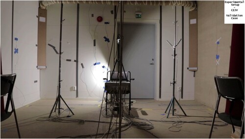
The experiment intended for the CFD validation was conducted in a medium-sized office room with the dimensions 7.2 × 4.1 × 2.7 m. The room contained two workstations, one facing the east side and one facing the west side as shown in Figure 1. The experimental room facing the south wall at which the inlets are located in the office mock-up room are shown in Figure 2. Each workstation contained an office chair, a desk and a seated thermal mannequin. The composition of the sidewalls was 15 mm wood sheet, 35 mm air gap, 15 mm wood sheet, 190 mm insulation and 5 mm wood sheet. The ceiling and the floor were insulated by 150 mm mineral wool. Since the walls on all side were well insulated and the temperature inside was close to the ambient external temperature, the heat transfer from this room to the laboratory hall was assumed minor. The office room was situated inside a spacious laboratory hall which kept a constant temperature of 23.6°C ± 0.6°C throughout the measurement period. The supply inlets were positioned at the corners of the south wall, with the main air inlet situated in the middle of the wall section. Air was delivered to each device through well-insulated ventilation tubes (20 mm mineral wool). The inlets were placed at a height of 0.8 m above the floor level, while the outlet was positioned at the centre near the north wall. Apart from the two thermal mannequins, two heat sources in the form of lamps were placed on the north side of the tables. To measure velocity and temperature, low-velocity omnidirectional thermistor anemometers were used. The thermistor and the logger system, CTA88, were designed and calibrated for velocities between 0.05 and 1.0 m/s. The velocity was measured with an accuracy of ±5%, ±0.05 m/s, excluding the directional error, directional sensitivity: 10% at angles within ±130° relative to the probe axis and the response time of 0.2 s to 90% of a step change. The uncertainty of temperature measurements was ±0.2°C with the response time of 12 s to 90% of value in still air. The measuring temperature range is 10–40°C. For a more comprehensive explanation of the measurement equipment and the uncertainty associated with the measurements, etc. see Ameen et al. (2019a). Measurements were conducted at various locations labelled as P1–P5, with measurements taken at different heights of 0.1, 0.6, 1.1 and 1.7 m. The supply air temperature was kept constant at 17°C, and a flow rate of 20 L/s was set for each inlet during the validation study. The thermal mannequins used in the experiment had the same surface area as a human (∼1.7 m²) and produced 100 W of heat in a seated position. Two enclosures containing halogen lamps generated 75 W of heat each, which were placed beside each desk as seen in Figure 1. Each inlet had a surface area of 0.0133 m² and had side dimensions of 0.163 × 0.163 × 0.231 m. In this study, sulphur hexafluoride (SF₆) was utilized as the tracer gas. To calculate the age of the air values, measurements were taken at six different locations in the room, including P1–P5 as depicted in Figure 1, at a height of 1.1 m as well as the outlet. Gas chromatography was utilized to measure the concentration of the gas in air samples, with three repetitions of each measurement to ensure validity. The average deviation among all three measurements ranged from 1% to 3%. The uncertainty of mean age of air measurements was ±2.5%, but this value could increase when accounting for airflow variation, pressure balancing, air leakage and other factors. The uncertainty of air change efficiency in this study complied with Appendix E of ASHRAE Standard 129 (ASHRAE, 1997). The total accumulated uncertainty of measured air change efficiency values was approximately 7%, based on minor air leakage and the measuring accuracy of the equipment. This outcome is consistent with previous laboratory studies (Buratti et al., 2011; Cehlin et al., 2019; Faulkner et al., 1995).

Figure 1. Measurement positions and schematic top-view layout of the mockup office room.

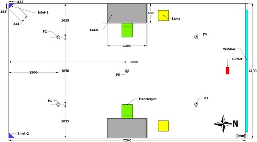
Figure 2. The office room showing the two CIJV inlets in the experimental validation setup.

2.2. Governing equations

The conservation laws of mass, momentum and energy equations were used to describe the airflow and temperature in the model. The simulations were conducted under certain assumptions and limitations, including three-dimensional, steady-state, incompressible and turbulent conditions. The momentum equation includes the buoyancy effect, and the density is governed by the incompressible ideal gas law, which only changes with temperature (ANSYS, 2020). The radiative heat fluxes within the computational domain were evaluated using the discrete ordinates (DO) radiation model. Specifically, this radiation model is founded on the conservative DO version, which employs the finite-volume method as outlined by Howell et al. (2020). This approach calculates the radiative transfer equation by considering a finite set of discrete solid angles (the number of equations considered aligns with the defined discrete solid angles). As a result, the radiative transfer equation is transformed into a standard transport equation, which is then solved numerically alongside the other equations that solve the other components in the domain. For the DO radiation model utilized, the solid angles are established through fixed vector directions within the spatial coordinates. This involves an angular discretization strategy grounded in control angles that dictate how each octant in the angular space is discretized. In this study the DO configuration in Fluent is set as follows; angular discretization is set to 2 theta divisions, 2 phi divisions, 1 theta pixels and 1 phi pixels. The energy iterations per radiation iteration is set to 1. Under these assumptions, the three-dimensional Reynolds time-averaged Navier-Stokes (RANS) equations are expressed as: (1) ${\displaystyle \frac{\mathrm{\partial }}{\mathrm{\partial }{x}_i}\left(\rho U_i\right)=0}$(1) (2) ${\displaystyle \frac{\mathrm{\partial }\left(\rho U_j{U}_i\right)}{\mathrm{\partial }{x}_j}=-{\displaystyle \frac{\mathrm{\partial }P}{\mathrm{\partial }{x}_i}+{\displaystyle \frac{\mathrm{\partial }}{\mathrm{\partial }{x}_j}\left(\mu {\displaystyle \frac{\mathrm{\partial }{U}_i}{\mathrm{\partial }{x}_j}-\rho \overline{u_i^{\mathrm{\prime }}}\overline{u_j^{\mathrm{\prime }}}}\right)+\left(\rho -{\rho }_0\right)g_i}}}$(2) (3) ${\displaystyle \frac{\mathrm{\partial }\left(\rho C_p{U}_{j}T\right)}{\mathrm{\partial }{x}_j}={\displaystyle \frac{\mathrm{\partial }}{\mathrm{\partial }{x}_j}\left(\lambda {\displaystyle \frac{\mathrm{\partial }T}{\mathrm{\partial }{x}_j}}\right)-{\displaystyle \frac{\mathrm{\partial }}{\mathrm{\partial }{x}_j}\left(\rho C_p\overline{u_j^{\mathrm{\prime }}{T}^{\mathrm{\prime }}}\right)}}}$(3) where $\rho$ is the density of the fluid, $U_i$ is the mean component of velocity in the direction $x_i$, $P$ is the pressure, $\mu$ is the dynamic viscosity and $u^{\mathrm{\prime }}$ is the fluctuating component of velocity.

In Equation (3) the Reynolds stresses $-\rho \overline{u_i^{\mathrm{\prime }}}\overline{u_j^{\mathrm{\prime }}}$ are given by the Boussinesq hypothesis: (4) $-\rho \overline{u_i^{\mathrm{\prime }}}\overline{u_j^{\mathrm{\prime }}}={\mu }_t\left({\displaystyle \frac{\mathrm{\partial }{U}_i}{\mathrm{\partial }{x}_j}+{\displaystyle \frac{\mathrm{\partial }{U}_j}{\mathrm{\partial }{x}_i}}}\right)-{\displaystyle \frac{2}{3}{\delta }_{ij}k}$(4) and (5) $-\rho C_p\overline{u_j^{\mathrm{\prime }}{T}^{\mathrm{\prime }}}={\displaystyle \frac{C_p{\mu }_t}{{\sigma }_t}{\displaystyle \frac{\mathrm{\partial }T}{\mathrm{\partial }{x}_j}}}$(5) where $k$ is the turbulent kinetic energy which is defined by $k={\displaystyle \frac{1}{2}\overline{u_i^{\mathrm{\prime }}}\overline{u_j^{\mathrm{\prime }}}}$, ${\mu }_t$ is the turbulent viscosity, ${\delta }_{ij}$ the Kronecker symbol; ${\delta }_{ij}$ = 1 if i = j and ${\delta }_{ij}$ = 0 if i≠j and ${\sigma }_t$ is turbulent Prandtl number. In order to calculate ${\mu }_t$ additional transport equations have to be considered. Depending on the type of turbulence model chosen this can vary. Evaluating previous studies in the same field show that several turbulence models have been successfully used to model IJV system. From previous research (Chen & Moshfegh, 2011; Hu et al., 2021a; Yakhot & Orszag, 1986; Ye et al., 2019) four models, Standard $k-ϵ$, RNG $k-ϵ$, Realizable $k-ϵ$ and SST $k-\omega$, were chosen which have yielded good results in predicting impinging jet air flow and temperature fields. Additionally, in the nearfield evaluation of CJIV (Ameen et al., 2022b), it was shown that RNG $k-ϵ$ was able to predict a CIJV configuration. Since the RNG $k-ϵ$ was chosen a more in-depth theoretical background is provided for this model. In the RNG $k-ϵ$ (Chen et al., 2013a; Hu et al., 2021b) model, ${\mu }_t$ is expressed as: (6) ${\mu }_t=\rho C_{\mu }{\displaystyle \frac{k^2}{ϵ}}$(6) The transport equation for the kinetic energy k and its dissipation rate $ϵ$ are as follows: (7) ${\displaystyle \frac{\mathrm{\partial }\left(\rho U_{j}k\right)}{\mathrm{\partial }{x}_j}={\displaystyle \frac{\mathrm{\partial }}{\mathrm{\partial }{x}_j}\left(\left(\mu +{\displaystyle \frac{{\mu }_t}{{\sigma }_k}}\right){\displaystyle \frac{\mathrm{\partial }k}{\mathrm{\partial }{x}_j}}\right)+{\mu }_t\left({\displaystyle \frac{\mathrm{\partial }{U}_i}{\mathrm{\partial }{x}_j}+{\displaystyle \frac{\mathrm{\partial }{U}_j}{\mathrm{\partial }{x}_i}}}\right){\displaystyle \frac{\mathrm{\partial }{U}_i}{\mathrm{\partial }{x}_j}+\text{β}{g}_i{\displaystyle \frac{{\mu }_t}{{\sigma }_t}{\displaystyle \frac{\mathrm{\partial }T}{\mathrm{\partial }{x}_i}-\rho ϵ}}}}}$(7) (8) ${\displaystyle \frac{\mathrm{\partial }\left(\rho U_jϵ\right)}{\mathrm{\partial }{x}_j}={\displaystyle \frac{\mathrm{\partial }}{\mathrm{\partial }{x}_j}\left(\left(\mu +{\displaystyle \frac{{\mu }_t}{{\sigma }_{ϵ}}}\right){\displaystyle \frac{\mathrm{\partial }ϵ}{\mathrm{\partial }{x}_j}}\right)+C_{1ϵ}{\displaystyle \frac{ϵ}{k}\left[{\mu }_t\left({\displaystyle \frac{\mathrm{\partial }{U}_i}{\mathrm{\partial }{x}_j}+{\displaystyle \frac{\mathrm{\partial }{U}_j}{\mathrm{\partial }{x}_i}}}\right){\displaystyle \frac{\mathrm{\partial }{U}_i}{\mathrm{\partial }{x}_j}+C_{3ϵ}\left(\text{β}{g}_i{\displaystyle \frac{{\mu }_t}{{\sigma }_t}{\displaystyle \frac{\mathrm{\partial }T}{\mathrm{\partial }{x}_i}}}\right)}\right]-C_{2ϵ}\rho {\displaystyle \frac{{ϵ}^2}{k}-{\displaystyle \frac{C_{\mu }\rho {\eta }^3\left(1-\eta /{\eta }_0\right)}{1+\text{β}{\eta }^3}{\displaystyle \frac{{ϵ}^2}{k}}}}}}}$(8) where $\eta =S\left(k/ϵ\right)$ describes the ratio between the time scales of the turbulence and the mean flow, S is the coefficient of surface tension. The constants used in the RNG $k-ϵ$ model are: $C_{\mu }$ = 0.0845, $C_{1ϵ}$ = 1.42, $C_{2ϵ}$ = 1.68, $C_{3ϵ}$ = $tanh\left(u_{par}/u_{per}\right)$, ${\sigma }_{ϵ}$ =  ${\sigma }_k$ = 0.7194, ${\sigma }_t$ = 0.85, $\text{β}$ = 0.012 and ${\eta }_0$ = 4.38.

2.3. Numerical setup and boundary conditions

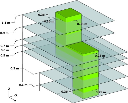
In this study, Ansys, 2020 R2 software was used to create the geometry, mesh and simulate the cases. Fluent 20.2.0, a finite-volume solver, was used with ‘coupled’ pressure-velocity coupling scheme and least squares cell-based method was used to solve the gradients. Second-order upwind discretization schemes were used for the pressure-term and the momentum-term, and an under-relaxation factor of 0.3 and 0.7 were used at the start of the simulations, respectively. The maximum relative difference between two consecutive iterations for all variables was set to less than 10⁻³ to achieve numerical convergence. The simulations were performed on a server with two AMD Epyc 7402 3.35 GHz processors, each with 24 cores. The enhanced wall treatment method was used to model the properties of turbulent flow in the near-wall regions. The inlet profile of the computational domain was set as a cyclic boundary condition, and the pressure outlet setting was used for the exhaust. Non-slip walls were set for all internal surfaces, while grey surfaces with an emissivity of 0.9 were assumed for all surfaces except for windows, computers, and mannequins, which were provided with constant heat flux. The thermal comfort and ventilation performance in a room are strongly influenced by the external environment. Therefore, accurate prediction of the heat flow was essential for setting up a precise computational fluid dynamics (CFD) model. In this study, IDA Indoor Climate and Energy 4.8 SP2 (IDA ICE) was employed to investigate the impact of external conditions on the examined room. IDA ICE is a building simulation software developed by the Royal Institute of Technology and the Swedish Institute of Applied Mathematics (Sahlin et al., 2004) and has been validated in a previous study by Woloszyn and Rode (2008). This software enables energy and indoor climate simulation for the entire building and is suitable for both large buildings with multiple zones and simple one-zone models, such as the one used in this study. IDA ICE is widely used in Nordic countries and Europe for energy performance estimates (Ahmed et al., 2018; Ameen et al., 2022a; Kristjansdottir et al., 2018; Pieskä et al., 2020) and comparison of energy performance in different climate regions (Soleimani-Mohseni et al., 2016). To evaluate various outdoor temperatures for winter and summer seasons, this research used IDA ICE simulation software's specific simulation functions for heating and cooling loads. Heat loads in the room were generated by occupants, computers, and office lamps. A synthetic weather condition was selected, which allowed for a fixed temperature to be set for the outdoor environment. The simulations took into account 100% of the internal heat gains, while assuming no impact from solar radiation by using internal blinds. The model included five internal walls, including the floor and ceiling, and one external wall facing the north side. Heat transfer was assumed to not occur through the internal walls, as it was assumed that the temperature on the other side was similar to that of an office indoor environment. The external wall featured a triple-pane window with a glazing area of 5.92 m², with a U-value of 1.2 W/(m² K) for the window and 0.18 W/(m² K) for the external wall. The simulations maintained consistent heat loads from occupants, computers, and lamps, with two occupants (100 W each), two computers (60 W each), and six lamps (20 W each). An imposed heat flux was applied to the external wall and window based on the outdoor temperature. The boundary conditions for the CFD model in Ansys Fluent were obtained from simulation results generated by IDA ICE software. A fixed supply air flowrate of 24.3 L/s (12.15 L/s for each inlet) was used for all cases, as per the recommended guidelines set by Boverket’s building regulations in Sweden (BBR) for an office room with two occupants. The supply air temperature was determined based on the outdoor environment, ranging from 12.5°C to 19°C. Using the method described, the operative temperatures for all cases studied were maintained within the range of 21–23°C for winter cases and 24–26°C for summer cases. The supply inlet temperature was chosen based on the target indoor temperature for winter and summer cases while minimizing energy usage. The aim was to achieve an indoor air temperature range of 21–26°C while minimizing energy consumption by keeping the inlet temperature as close as possible to the outdoor temperature. Multiple IDA ICE simulations were performed in an iterative process to achieve this. For the CFD simulations, a symmetry plane was placed in the centre of the model to reduce simulation time and computational resources. Figure 3 shows the areas of interest, located at 0.1, 0.3, 0.5, 0.6, 0.7, 0.9 and 1.1 m above the floor. 1.1 m was considered to be at the face level of a person sitting in an office environment. Thermal comfort and indoor air quality indices were evaluated in these areas to assess the effectiveness of the ventilation system.

Figure 3. Evaluated areas around the mannequin at various heights.

2.4. Mesh strategy and mesh independence study

For this study, a non-uniform grid distribution was used. The mesh was refined around the inlet, walls and object inside the room. Ansys Icepak 2020 R2 was used to create the mesh, and three different mesh densities were tested and compared. Three different mesh densities were tested and evaluated. The number of structured hexahedral cells contained within these models were 13.56 (coarse), 19 (medium) and 26.58 (fine) million. The RNG $k-ϵ$ turbulence model was used, with the enhanced wall treatment method applied for the near-wall modelling, see ANSYS Fluent Tutorial Guide (ANSYS, 2020). The authors concluded that since all chosen models for validation were RANS-based, testing other models would not significantly impact the outcome of the mesh independency test, see (Chen et al., 2012). The differences between the mesh densities were evaluated by comparing temperature and velocity measurements at various points within the office room. The root-mean-square error (RMSE) was computed using Equation 9, based on data collected from 1335 measurement points located at P1–P5. At each of the five locations 267 measuring positions were evaluated and data extracted. In Equation 9 n is the total number of selected measuring points (267) and ${\varphi }_{in}$ is the nominal inlet velocity or the inlet temperature depending on what physical parameter was evaluated. For velocity ${\varphi }_{in}$ = 1.5 m/s and for temperature ${\varphi }_{in}$ = 17°C. ${\varphi }_{i,BG}$ is the numerical solution at base grid resolution (lower cell count) and ${\varphi }_{i,RG}$ is the numerical solution at refined grid resolution (higher cell count). 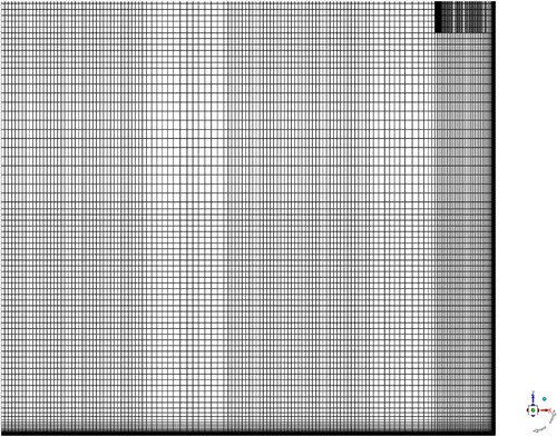(9) $RMSE=\sqrt{{\displaystyle \frac{1}{n}\sum _{i=1}^n{\left({\displaystyle \frac{{\varphi }_{i,BG-}{\varphi }_{i,RG}}{{\varphi }_{in}}}\right)}^2}}$(9) The result of this evaluation showed a small gain between the fine and medium model, that had 19 and 26.58 million cells respectively. The difference between coarse model (13.56 million) and the medium (19 million) was 4.1% when comparing temperature and 0.4% when comparing velocity measurements. These were 2.8% and 0.4% for temperature and velocity respectively between the medium and fine model, hence the medium model with 19 million cells was chosen for the numerical study. Figure 4–6 visualizes the final mesh from different angles and directions.

Figure 4. Isometric view over the mesh in the office room.

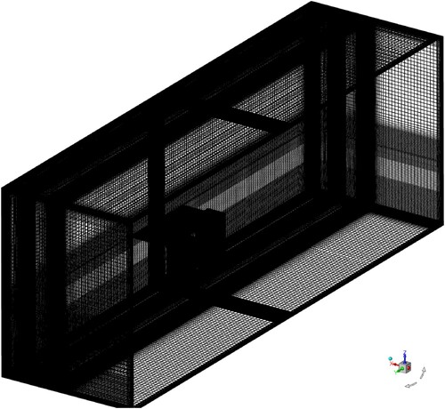
Figure 5. Mesh view in the x-direction directly below the inlet.

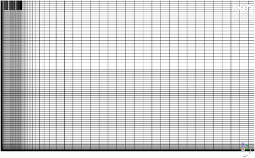
Figure 6. Mesh view in the y-direction directly below the inlet.

The dimensionless wall distance, y⁺, is used to accurately describe the turbulence flow in the vicinity of the walls and defined by: (10) $y^{+}={\displaystyle \frac{\mathrm{\Delta }y}{\nu }\sqrt{{\displaystyle \frac{{\tau }_w}{\rho }}}}$(10) where $\mathrm{\Delta }y$ is the vertical distance from wall to the first grid point, $\nu$ is the kinematic viscosity, $\rho$ is the fluid density and ${\tau }_w$ is the wall shear stress. The refined mesh resulted in an average y⁺ ≤ 1 on all walls and floor.

2.5. Model validation

Figure 7(a–j) presents a comparison of simulation results obtained using four turbulence models, namely Standard $k-ϵ$, RNG $k-ϵ$, Realizable $k-ϵ$ and SST $k-\omega$, with the experimental measurements. The evaluation of results was performed at various locations (P1–P5) indicated in Figure 1. For validation purposes, triangle-shaped inlets were used, with an inlet area of 0.0133 m² and side dimensions of 0.163 × 0.163 × 0.231 m. The measurements were taken at heights of 0.1, 0.6, 1.1 and 1.7 m. The validation study was carried out at a supply air temperature of 17°C and a total flow rate of 20 L/s, with each inlet receiving a flow rate of 10 L/s. During the experiment, mannequins with the same surface area as a human were used, with each mannequin producing 100 W of heat while in a sitting position. Additionally, two enclosures containing halogen lamps, each generating 75 W of heat, were placed at the sides of each desk. The results demonstrate that the predicted jet profiles are consistent across all the tested models. While there were some variations in accuracy across different regions, the predictions obtained using the four turbulence models were largely similar, with some models exhibiting slightly better accuracy than others. As an example, the SST $k-\omega$ model slightly underestimates the temperature at h = 0.1 m in P1, P2 and P3. Similar results have been observed in previous research when comparing the RNG $k-ϵ$ and SST $k-\omega$ models (Chen et al., 2012). It’s noteworthy that the airflow is not entirely stable, and fluctuations can occur in the flow field, as demonstrated in other studies (Cehlin & Moshfegh, 2010). Despite this, all four turbulence models provide temperature and velocity predictions that agree well with the measurements. To compute the RMSE for the turbulence models in comparison to the experimental data, Equation (9) was used. To perform this computation, temperatures and velocities recorded in the experimental arrangement (at heights of 0.1, 0.6, 1.1 and 1.7 m in P1–P5) were compared at the identical points for each turbulence model. The outcomes indicated an RMSE of 1.05% for RNG $k-ϵ$, 1.27% for Realizable $k-ϵ$, 1.12% for Standard $k-ϵ$ and 1.57% for SST $k-\omega$ for the temperature measurements. For the velocity measurements the results showed an RMSE value of 1.28% for RNG $k-ϵ$, 1.40% for Realizable $k-ϵ$, 1.30% for Standard $k-ϵ$ and 1.50% for SST $k-\omega$. Besides temperature and velocity, air change efficiency (ACE) was compared against the experimental outcomes. These measurements were taken at a height of 1.1 m in P1–P5 and are presented in Table 1. Only the RNG $k-ϵ$ turbulence model was employed to evaluate ACE. The comparison between the simulated and experimental results displayed a minor underestimation in the simulated results. Consequently, the RNG $k-ϵ$ model was chosen as the most suitable turbulence model for this study. This model demonstrated overall good performance when compared to the experimental data, and it has been widely employed in various numerical studies to simulate and predict impinging jet flow fields (Abbas, 2018; Chen et al., 2013a; Chen & Moshfegh, 2011; Hu et al., 2021a; Koufi et al., 2017; Staveckis & Borodinecs, 2021; Yang et al., 2021; Ye et al., 2016, 2020).

Figure 7. (a–j) Temperature and velocity profile comparisons for different turbulence models and experimental measurements at different locations (P1–P5).

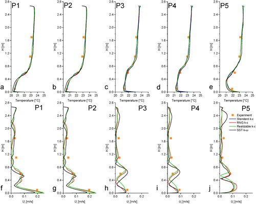
Table 1. ACE comparison between experimental and CFD at five locations.

	Experimental	CFD (RNG $k-ϵ$)	Difference (%)
P1 (@1.1 m)	1.35	1.32	2.2
P2 (@1.1 m)	1.36	1.32	2.9
P3 (@1.1 m)	1.39	1.36	2.2
P4 (@1.1 m)	1.38	1.36	1.5
P5 (@1.1 m)	1.19	1.18	0.5

2.6. Case studies

A total of 15 cases were simulated to investigate the effects of different outdoor environment and supplied air temperature have on the thermal and ventilation performance of the CIJV system, as shown in Table 2. All cases used the same supply flowrate of 24.3 L/s. The 15 cases were divided into 9 winter cases and 6 summer cases. A heat flux was imposed on the window and external wall as shown in Table 2. Heat loads from occupants, computers and lamps were the same for all the simulations, two occupants (100 W each), two computers (60 W each) and 6 lamps (20 W each). One CIJV inlet configurations was tested for each external temperature. The size of the inlet configuration was 0.00665 m². For each outdoor temperature, 3 different workspace location were evaluated, L-1, 1.8 m from the south wall, L-2 in the centre of the room at 3.6 m from the south wall and L-3, 5.4 m from the south wall as seen in Figure 8.

Figure 8. Workspace locations evaluated at 3 positions L-1, L-2 and L-3.

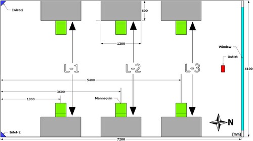
Table 2. Case conditions and parameter settings when evaluating the impact of different outdoor environment and supplied air temperature.

Cae	Workspace distance from south wall (m)	To (°C)	Ts (°C)	Uin (m/s)	Heat loss exterior wall and window (W)	Heat source from Occupant, Computer and Lighting (W)
Winter (heating)
Case 01	1.8	−15	19	1.84	−314	440
Case 02	3.6	−15	19	1.84	−314	440
Case 03	5.4	−15	19	1.84	−314	440
Case 04	1.8	−5	17	1.84	−238	440
Case 05	3.6	−5	17	1.84	−238	440
Case 06	5.4	−5	17	1.84	−238	440
Case 07	1.8	5	14	1.84	−156	440
Case 08	3.6	5	14	1.84	−156	440
Case 09	5.4	5	14	1.84	−156	440
Summer (cooling)
Case 10	1.8	15	15	1.84	−100	440
Case 11	3.6	15	15	1.84	−100	440
Case 12	5.4	15	15	1.84	−100	440
Case 13	1.8	25	12.5	1.84	−19	440
Case 14	3.6	25	12.5	1.84	−19	440
Case 15	5.4	25	12.5	1.84	−19	440

2.7. Evaluation indices

A quantitative assessment of the thermal comfort and indoor air quality (IAQ) performance of the CIJV using several key indices was carried out in this study. The evaluation of these indices was concentrated in the working zone area of the occupants, which we defined as a 1 m² area surrounding the occupant. With the working area established the height of 0.1, 0.3, 0.5, 0.6, 0.7, 0.9 and 1.1 m were used to extract the relevant data needed for all the indices.

2.7.1. Vertical temperature difference

One index that is commonly used to evaluate the local thermal comfort is the vertical temperature difference between head and ankle level. According to ASHRAE Standard 55-2020 (American Society of Heating and Refrigerating and Air-Conditioning Engineers, 2021), this difference should not exceed 3°C when measuring between occupants’ ankle level at 0.1 m above the floor, and the head level at 1.1 m for a seated person. This is calculated as: (11) $\mathrm{\Delta }{T}_{1.1-0.1}=T_{1.1}-T_{0.1}$(11) where $\mathrm{\Delta }{T}_{1.1-0.1}$ is the temperature difference between head and ankle level for a seated person. This index is important to evaluate due to the nature of the air stratification when using this type of ventilation system which typically creates a strong stratification in the occupied space compared to mixing ventilation, especially in cooling mode (Ameen et al., 2019a).

2.7.2. Draught rate

Another index is draught rate (DR) which describes the discomfort a person is feeling due to unwanted cooling of the human body. This index is a function of air velocity, temperature and turbulence intensity. DR predicts the percentage of dissatisfaction due to draft. According to ISO 7730-2005 (ISO 7730, 2005) DR is calculated as: (12) $\mathrm{D}\mathrm{R}=\left(3.14+0.37\cdot U_i\cdot I_l\right)\cdot \left(34-T_a\right)\cdot (u_m-0.05{)}^{0.62}$(12) $\mathrm{F}\mathrm{o}\mathrm{r}{U}_i<0.05\mathrm{m}/\mathrm{s}\mathrm{u}\mathrm{s}\mathrm{e}{U}_i=0.05\mathrm{m}/\mathrm{s}$ $\mathrm{F}\mathrm{o}\mathrm{r}DR>100\text{\%}\mathrm{u}\mathrm{s}\mathrm{e}DR=100\text{\%}$where $U_i$ is the mean air velocity, $I_l$ is the local turbulence intensity and $T_a$ is the local temperature. In term of thermal environmental classifications for DR, ISO 7730-2005 gives three categories. Category A which is best requires a DR < 10%, B requires DR < 20% and the lowest is C which requires DR < 30%. In this study, the DR is evaluated at ankle level (H = 0.1 m).

2.7.3. PMV and PPD

The predicted mean vote (PMV) is one of the most widely used indices for assessing thermal comfort. This model accounts for several factors, including air temperature, mean radiant temperature, air velocity, relative humidity, metabolic rate and clothing insulation, to approximate an individual's thermal sensation in the occupied space. PMV is defined in ASHRAE 55-2020 (American Society of Heating and Refrigerating and Air-Conditioning Engineers, 2021). The PMV model uses a scale from −3 to +3, where −3 indicates extreme cold, 0 indicates neutral, and +3 indicates extreme heat. A PMV value of 0 indicates that the environment is in thermal neutrality, meaning the individual is neither feeling hot nor cold and is thermally comfortable. PMV is typically evaluated at the height of 1.1 m (at head level) above floor level close to the occupant for a seated person. The MET value used for calculating PMV was set to 1.0 and CLO was set between 0.5 and 1.0 depending on outdoor weather conditions. The humidity value was set to 50% for all cases. PPD is an index that predicts quantitively the percentage of thermally dissatisfied people who feel too cool or too warm. At 5% the occupant is at thermal equilibrium which corresponds to PMV 0 and higher level of PPD indicates that the occupant feels either too cold or too warm. PPD is a function of PMV and is calculated by: (13) $\mathit{P}PD=\mathbf{100}\mathbf{-}\mathbf{95}\cdot {\mathit{e}}^{-\left(\mathbf{0.03353}\cdot \mathit{P}\mathbf{M}{\mathit{V}}^{\mathbf{4}}\mathbf{+}\mathbf{0.2179}\cdot \mathit{P}\mathbf{M}{\mathit{V}}^{\mathbf{2}}\right)}$(13) The PMV and PPD results were calculated by extracting the necessary parameters such as the horizontal average mean air temperature, horizontal average mean radiant and horizontal average mean air velocity for each specific plane at different heights which is shown in Figure 2. In Ansys Fluent the radiation temperature is defined as (ANSYS, 2020): (14) ${\mathit{\theta }}_{\mathit{R}}={\left({\displaystyle \frac{\mathit{G}}{\mathbf{4}\mathit{\sigma }}}\right)}^{\mathbf{1}\mathbf{/}\mathbf{4}}$(14) where G is the incident radiation in W/m², and $\sigma$ = 5.669 × 10⁻⁸ ${\displaystyle \frac{\mathrm{W}}{{\mathrm{m}}^2\times {\mathrm{K}}^4}}$ is the Stefan–Boltzmann constant. This data together with the MET and CLO value was used in the CBE thermal comfort tool (Tartarini et al., 2020) in order to obtain the PMV and PPD value.

2.7.4. Mean age of air and air change effectiveness

The air quality for CIJV during heating and cooling was evaluated using mean age of air and ACE. The local mean age of air is the average time for the air to move from the supply inlet entrance to a specific location in the ventilated space (Li et al., 2003). The transport equation used for mean age of air is defined as (Li et al., 2003; Ye et al., 2020): (15) ${\displaystyle \frac{\mathbf{\partial }\left(\mathit{\rho }{\mathit{u}}_{\mathit{i}}\mathit{\tau }\right)}{\mathbf{\partial }{\mathit{x}}_{\mathit{i}}}={\displaystyle \frac{\mathrm{\partial }}{\mathbf{\partial }{\mathit{x}}_{\mathit{i}}}\cdot \left[\left(2.88\mathit{\rho }\cdot {10}^{-5}+{\displaystyle \frac{{\mathit{\mu }}_{\mathit{e}ff}}{\mathit{S}{\mathit{c}}_{\mathit{\tau }}}}\right)\cdot {\displaystyle \frac{\mathbf{\partial }\mathit{\tau }}{\mathbf{\partial }{\mathit{x}}_{\mathit{i}}}}\right]+{\mathit{S}}_{\mathit{\tau }}}}$(15) where ${\mu }_{\mathrm{e}\mathrm{f}\mathrm{f}}$ is the effective turbulent viscosity of air, τ represents the local age of air and $\mathrm{S}{\mathrm{c}}_{\tau }$ is the turbulent Schmidt number of the age of air. Here $\mathrm{S}{\mathrm{c}}_{\tau }$ = 0.7. The source term ${\mathrm{S}}_{\tau }$ is commonly set with the fix value of 1.0. In Ansys fluent a user-defined scalar (UDS) was used in order to calculate the mean age of air. ACE was used as an indicator to investigate the capability of CIJV to deliver fresh air into the occupied zone. ACE is defined as the ratio of the nominal time to mean age of air in the occupied zone (Fan et al., 2017). (16) $\mathrm{A}\mathrm{C}\mathrm{E}={\displaystyle \frac{{\tau }_n}{\tau }}$(16) where ${\tau }_n$ and $\tau$ denotes in (s). The nominal time constant ${\tau }_n$ is defined as: (17) ${\tau }_n={\displaystyle \frac{V_{room}}{q_i}}$(17) where $V_{room}$ is the room volume (m³) and $q_i$ is the inlet supply air flowrate (m³/s). ${\tau }_n$ is the arithmetic average age of air for a defined horizontal area (see Figure 2). The value of ACE = 1.0 indicates a fully mixed air in the room. According to (ASHRAE, 1997; Fan et al., 2017) the minimum recommended value of ACE should be 0.95, which can provide an adequate level of IAQ in the occupied zone, and a higher value of ACE means better IAQ.

3. Results and discussion

3.1. Results for indoor thermal comfort

3.1.1. Characteristics of the temperature field

Figure 9(a) shows the results of the horizontal average temperature profiles at the height of 0.1–1.1 m for all winter cases (Cases 1–9). The results for Case 1 (L-1 position) showed a fairly uniform temperature between 22.9°C and 23.3°C at the height between 0.1 and 0.6 m. Higher up, between 0.6 and 0.9 m the temperature for Case 1 increased up to almost 24.7°C and at head level (H = 1.1 m) the temperature was around 23.6°C. The results for Case 2 (L-2 position) showed a fairly uniform temperature between 22.9°C and 23.2°C at the height between 0.1 and 0.6 m. Higher up, between 0.6 and 0.9 m the temperature for Case 1 increased up to almost 24.2°C and at head level (H = 1.1 m) the temperature was around 23.7°C. The results for Case 3 (L-3 position) showed a fairly uniform temperature between 22.7°C and 23.0°C at the height between 0.1 and 0.6 m. Higher up, between 0.6 and 0.9 m the temperature for Case 1 increased up to almost 23.9°C and at head level (H = 1.1 m) the temperature was around 23.4°C. The results showed that the overall temperature was slightly colder if the workspace is closer to the window than compared to the centre or close to the south wall. At head level (H = 1.1 m) the difference between Case 1 and Case 3 was 0.2°C. When evaluating Cases 4–6 when the outdoor temperature has increased by 10°C to −5°C, a similar development has occurred, with Case 6 (L-3) having a slightly colder temperature except at 0.1 m where it is slightly lower (0.3°C) that Cases 4 and 5. This trend was still maintained when evaluating Cases 7–9. Figure 9(b) shows the results of the temperature profiles at the height of 0.1–1.1 m for all summer cases (Cases 10–15). In the summer cases the ventilation system was switched to cooling mode instead of heating and consequently a higher temperature setpoint was adapted. The results for Case 10 (L-1 position) showed a temperature range between 24.3°C and 25.9°C at the height between 0.1 and 0.6 m. Higher up, between 0.6 and 0.9 m the temperature for Case 10 increased up to almost 27.4°C and at head level (H = 1.1 m) the temperature was around 26.3°C. The results for Case 11 (L-2 position) showed a temperature range between 24.8 and 25.8°C at the height between 0.1 and 0.6 m. Higher up, between 0.6 and 0.9 m, the temperature for Case 11 increased up to almost 26.8°C and at head level (H = 1.1 m) the temperature was around 26.3°C. The results for Case 12 (L-3 position) showed a temperature range between 24.8°C and 25.5°C at the height between 0.1 and 0.6 m. Higher up, between 0.6 and 0.9 m the temperature for Case 1 increased up to almost 26.3°C and at head level (H = 1.1 m) the temperature was around 25.9°C. The results once again showed that the overall temperature is slightly colder if the workspace is closer to the window than compared to the centre or close to the south wall for H ≥ 0.6 m. At head level (H = 1.1 m). When evaluating the final 3 summer cases, the results showed a deviation from the previous trends.

Figure 9. (a) Shows the horizontal averaged temperatures at different heights in the occupied zone (See Figure 2) for winter cases and (b) for summer cases.

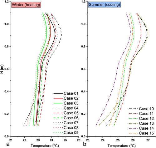
The results for Case 13 (L-1 position) showed an overall warmer temperature except at the lower parts at H = 0.1 m. The results also showed that Case 15 (L-3 position) was now slightly warmer than warmer than Case 14 (L-2 position). The reason for this was that the room was now supplied with cold air at at 12.5°C with made the south side room colder than the north side which now faced a wall that was connected to an outdoor temperature of 25°C. The results also showed that the temperature stratification was increasing as the outdoor temperature was increased.

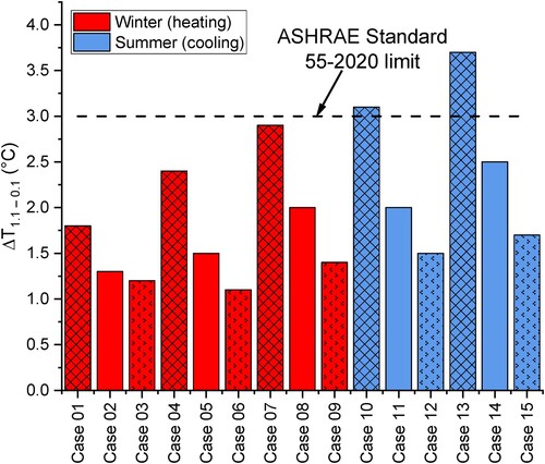
In order to quantify the temperature stratification, Figure 10 shows the temperature difference between head and ankle level (1.1–0.1 m). The figure also shows the maximum limit that ASHRAE Standard 55-2020 (American Society of Heating and Refrigerating and Air-Conditioning Engineers, 2021) allows for temperature difference between these levels, which is 3°C. When evaluating Cases 1–3 the results showed that the temperature differences were below of the ASHRAE limit, at around 1.8°C for Case 1 (L-1 position), 1.3°C for Case 2 (L-2 position) and 1.2°C for Case 3 (L-3 position). These results were slightly increased for Cases 4, 5 to 2.4, 1.5°C and but stayed almost the same at 1.1°C for Case 6. For Cases 7, 8 and 9 the results showed 2.9, 2.0 and 1.4°C respectively. This trend is continued when evaluating the summer cases with increased temperatures for Cases 10, 11 and 12 which showed 3.1, 2 and 1.5°C respectively and for Cases 13, 14 and 15 that showed 3.7, 2.5 and 1.7°C respectively. There results show a clear temperature stratification which is strengthen by increased outdoor temperature. It is also worth noting that for Cases 10 and 13 which is L-1 (close to the inlets) the temperature difference exceeds the limit of 3°C set by ASHRAE. However, this overreach is very small, for Case 10 the results showed 0.1°C and for Case 13, 0.7°C. These results are similar to previous research that have showed how impinging jet ventilation creates temperature stratification depending on if it was working in heating mode (Ameen et al., 2019b; Hu et al., 2021b; Ye et al., 2019, 2022) or in cooling mode (Ameen et al., 2019a; Chen et al., 2013b; Hu et al., 2021a). As the room requirement (i.e. how much heating or cooling is required and supply air temperature) changes depending on the outdoor temperature so does the room temperature stratification. In general, the CIJV has less temperature stratification when working heating mode, which the system behaves similar to MV. However, when working in cooling mode the CIJV creates a clear stratification in the occupied region.

Figure 10. The temperature difference between the height of 1.1 and 0.1 m in the occupied zone for all cases.

3.1.2. Evaluation of thermal comfort and draft sensation

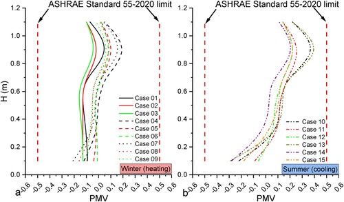
Figure 11(a) shows the results of PMV at the height of 0.1–1.1 m for all winter cases (Cases 1–9). The results for Cases 1–3 showed a PMV level that is within the acceptable range of −0.16 to 0.1. This value was within the acceptable thermal comfort range of ≥−0.5 to ≤0.5 set by ASHRAE Standard 55-2020 (American Society of Heating and Refrigerating and Air-Conditioning Engineers, 2021). Continuing to the next set of cases (Cases 4–6) the results showed a slight increase in PMV for all the cases (−0.12 to 0.26). Cases 7–9 showed a similar result compared to Cases 4–6 (−0.21 to 0.22). Evaluating the rest of the summer cases (Cases 10–15 in Figure 11(b)) for summer conditions, the results showed that the PMV values were kept within the recommended value with the lowest recorded value registered for Case 14 (0.03), and highest by Case 13 (0.49). When evaluating the summer cases, the PMV results showed how the temperature stratification affected PMV results. At lower heights (H = 0.1) where fresh (and colder) air was supplied by the ventilation system to the room, the PMV value gravitated towards the colder side (PMV < 0) even during the summer period as shown in Figure 11(b).

Figure 11. (a) Shows the horizontal averaged PMV level at different heights in the occupied zone (See Figure 2) for winter cases and (b) for summer cases.

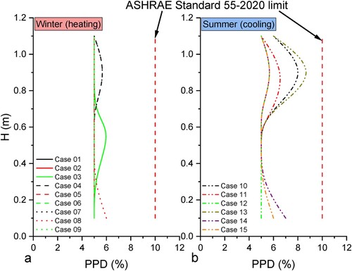
The PMV results are strongly affected by the temperature profiles shown in Figure 9. When evaluating the PPD levels the result showed that all the cases (Cases 1–15) were all below the limit of 10% which is stipulated by the ASHRAE Standard as shown in Figure 12(a,b). However, the PPD values were elevated for several cases at lower heights H = 0.1 m and at H = 0.9 m. When evaluating the winter cases as shown in Figure 12(b), the results showed higher PPD level than compared to the summer cases, especially at H = 0.9 m. Still, these values are below the limit of 10% which counts as an acceptable thermal comfort level of the occupants. The predominant reason for this is the high temperature at this height in the summer cases.

Figure 12. (a) Shows PPD level at different heights in the occupied zone for winter cases. (b) Shows PPD level at different heights in the occupied zone for summer cases.

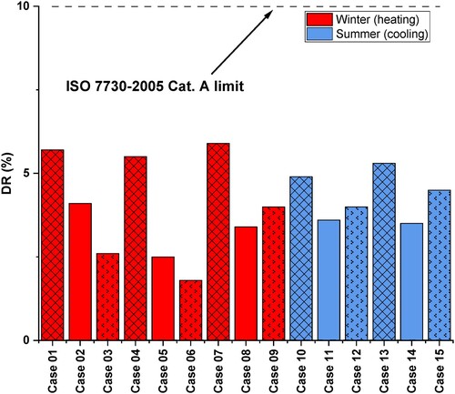
When evaluating the draught level at ankle level (H = 0.1 m) as seen in Figure 13, the results showed that the DR levels were below 5% for all cases, both during winter and summer. The results for the winter cases (Cases 1–9) showed a slightly higher level of DR for all cases close to the inlet (L-1 cases). This is related to the high velocity jet exiting the inlets and flowing towards the mannequins. As the distance becomes greater the jet loses its momentum and the velocity is reduced which in turn reduces the draught rate sensation. However, the results for the summer cases (Cases 10–15) showed a much more uniform level of DR. The authors believe that this is due to that in summertime the jet from the inlet is not affected as much by the buoyancy force as with the winter cases and hence it can travel much further into the room when compared to wintertime.

Figure 13. Shows the DR level at H = 0.1 m for all cases.

3.2. Results for indoor air quality

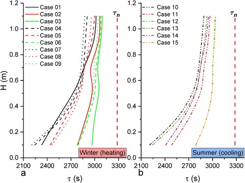
Figure 14(a) shows the results of the mean age of air (τ) for the winter cases (Cases 1–9). When evaluating Cases 1–3 the results showed a lower τ for Case 1(L-1 position) at 2330 s at H = 0.1 m compared to 2783 s for Case 2 (L-1 position) and 2966 s for Case 3 (L-3 position). Since Case 1 is closer to the inlet this development is not a surprise. However, when evaluating at higher levels, specifically at the breathing level the difference in τ is reduced considerably. At the height of H = 1.1 m, the results for Cases 1, 2 and 3 showed 3017, 3063 and 3095 s, respectively. Evaluating Cases 4, 5 and 6 at 1.1 m the results showed 2905, 2997 and 3080 s, respectively, which is lower than the nominal time constant τ_n which in this study was 3280 s. Looking at Cases 7, 8 and the results showed 2874, 2959 and 3044 s, respectively. These results show that τ during wintertime is lower than the τ_n. The results also show that at the critical level of 1.1 m L-1 Cases have better values compared to L-2 and L-3 cases and L-3 has the worst. These results can be contributed to the distance the workstations have from the inlets. A similar development can be seen with the summer cases that is shown in Figure 14(b). The results for Cases 10, 11 and 12 at the height of 1.1 m were 2891, 2968 and 3039 respectively. The results for Cases 13, 14 and 15 at the height of 1.1 m were 2930, 2950 and 3032 respectively. The values, both for summer and winter cases, were all below the τ_n which indicates a potential for energy saving in future studies.

Figure 14. (a) Shows the horizontal averaged τ at different heights in the occupied zone for winter cases and (b) for summer cases.

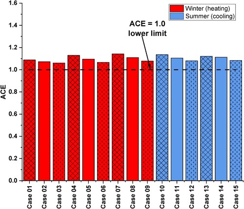
Figure 15 shows the ACE value at H = 1.1 m for all cases (Cases 1–15) for both heating and cooling season. The results of ACE value showed that the ACE value was consistently over 1.0 limit, which showed that this system was efficient both during summer and winter conditions. When evaluating Cases 1, 2 and 3 the results showed an ACE value of 1.09, 1.07 and 1.06, respectively. The ACE results for Cases 4, 5 and 6 were 1.13, 1.10 and 1.07 respectively. The ACE results for Cases 7, 8 and 9 were 1.14, 1.11 and 1.08, respectively. For the summer cases (Cases 10–15) the ACE results are very similar to Cases 7–9. It is worth noting that having the workspace close to the inlet device (L-1 cases) yields a slightly higher ACE value compared to L-2 and L-3 cases. The L-3 cases showed the worst ACE performance, and the L-2 ends up in the middle. Even though the results are in favour of having the workspace closer to the inlets it is still possible to place them close to the external wall as well since the difference in ACE between each position is small. The largest difference between L-1 and L-3 cases is 0.06 which is between Cases 4 and 6, Cases 7 and 9 and Cases 10 and 12. These ACE results are in line with other studies that have concluded that ACE >1.0 for air distribution systems based on impinging ventilation (Ameen et al., 2019b, 2019a; Ye et al., 2020).

Figure 15. Shows the ACE at head level (H = 1.1 m) for all cases.

4. Conclusion

This study aimed to investigate the feasibility of using corner impinging jet ventilation (CIJV) as the sole method for heating and cooling a medium-sized office space with two occupants while maintaining adequate indoor thermal comfort and air quality compared to traditional mixing systems. The study examined the impact of various outdoor temperatures ranging from −15°C (winter) to 25°C (summer) on the office environment using a parametric setup with fixed ventilation flowrate (24.3 L/s) and specific heating loads. Three different workspace locations were evaluated, one close to the inlet, one in the middle of the room and one far away.

The results showed that the CIJV system met ASHRAE thermal comfort standards, with acceptable levels of PMV, PPD, DR. For ΔT_1.1–0.1 all cases were below the 3°C threshold except for the two summer cases in which the workstation was closest to the inlets. In terms of indoor air quality, CIJV performed better than traditional mixing systems, with improved τ and ACE values. Temperature stratification was stronger in the summer compared to winter. This study concluded that CIJV can be used for all three evaluated workspace locations (1.8, 3.6 and 5.4 m from the inlet) in terms of thermal comfort and indoor air quality both during cooling and heating season.

Declaration of competing interest

The authors declare that they have no known competing financial interests or personal relationships that could have appeared to influence the work reported in this paper.

Disclosure statement

No potential conflict of interest was reported by the author(s).

Data availability

Data will be made available on request by contacting the corresponding author.

Additional information

Funding

Internal research funding from the University of Gävle.

References

- Abbas, S. M. (2018). Experimental and theoretical investigation of impinging jet ventilation at different cross sectional area of supply air duct. Journal of University of Babylon for Engineering Sciences, 26(5), 238–257. https://www.journalofbabylon.com/index.php/JUBES/article/view/1033
- Ahmed, K., Carlier, M., Feldmann, C., & Kurnitski, J. (2018). A new method for contrasting energy performance and near-zero energy building requirements in different climates and countries. Energies, 11(6), 1334. https://doi.org/10.3390/en11061334
- Ameen, A., Bahrami, A., & El Tayara, K. (2022a). Energy performance evaluation of historical building. Buildings, 12(10), 1667. https://doi.org/10.3390/buildings12101667
- Ameen, A., Cehlin, M., Larsson, U., & Karimipanah, T. (2019a). Experimental investigation of the ventilation performance of different air distribution systems in an office environment – cooling mode. Energies, 12(7), 1354. https://doi.org/10.3390/en12071354
- Ameen, A., Cehlin, M., Larsson, U., & Karimipanah, T. (2019b). Experimental investigation of ventilation performance of different air distribution systems in an office environment-heating mode. Energies, 12(10), 1835. https://doi.org/10.3390/en12101835
- Ameen, A., Cehlin, M., Larsson, U., Yamasawa, H., & Kobayashi, T. (2022b). Numerical investigation of the flow behavior of an isothermal corner impinging jet for building ventilation. Building and Environment, 223, 109486. https://doi.org/10.1016/j.buildenv.2022.109486
- Ameen, A., Yamasawa, H., & Kobayashi, T. (2022c). Numerical evaluation of the flow field of an isothermal dual-corner impinging jet for building ventilation. Buildings, 12(10), 1767. https://doi.org/10.3390/buildings12101767
- American Society of Heating and Refrigerating and Air-Conditioning Engineers. (2017). Thermal environmental conditions for human occupancy: ANSI/ASHRAE standard 55-2017. ASHRAE Peachtree Corners, GA, USA.
- American Society of Heating and Refrigerating and Air-Conditioning Engineers. (2021). Thermal environmental conditions for human occupancy: ANSI/ASHRAE standard 55-2020. ASHRAE Peachtree Corners, GA, USA.
- ANSYS. (2020). ANSYS fluent theory guide 2020 R2. In ANSYS Inc. ANSYS, Inc. Canonsburgh, PA, USA.
- ASHRAE, A. S. (1997). Standard 129-1997. Measuring air-change effectiveness, AHSRAE, Atlanta, GA.
- Awbi, H. B. (2002). Ventilation of buildings. Routledge.
- Buratti, C., Mariani, R., & Moretti, E. (2011). Mean age of air in a naturally ventilated office: Experimental data and simulations. Energy and Buildings, 43(8), 2021–2027. https://doi.org/10.1016/j.enbuild.2011.04.015
- Cao, G., Awbi, H., Yao, R., Fan, Y., Sirén, K., Kosonen, R., & Zhang, J. J. (2014). A review of the performance of different ventilation and airflow distribution systems in buildings. Building and Environment, 73, 171–186. https://doi.org/10.1016/j.buildenv.2013.12.009
- Cehlin, M., Karimipanah, T., Larsson, U., & Ameen, A. (2019). Comparing thermal comfort and air quality performance of two active chilled beam systems in an open-plan office. Journal of Building Engineering, 22. https://doi.org/10.1016/j.jobe.2018.11.013
- Cehlin, M., & Moshfegh, B. (2010). Numerical modeling of a complex diffuser in a room with displacement ventilation. Building and Environment, 45(10), 2240–2252. https://doi.org/10.1016/j.buildenv.2010.04.008
- Chen, H., Janbakhsh, S., Larsson, U., & Moshfegh, B. (2015). Numerical investigation of ventilation performance of different air supply devices in an office environment. Building and Environment, 90, 37–50. https://doi.org/10.1016/j.buildenv.2015.03.021
- Chen, H., & Moshfegh, B. (2011). Comparing k-ϵ models on predictions of an impinging jet for ventilation of an office room. The 12th International Conference on Air Distribution in Rooms, Trondheim, Norway June 19-22, 2011. https://www.diva-portal.org/smash/get/diva2:450171/FULLTEXT01.pdf
- Chen, H., Moshfegh, B., & Cehlin, M. (2013b). Computational investigation on the factors influencing thermal comfort for impinging jet ventilation. Building and Environment, 66, 29–41. https://doi.org/10.1016/j.buildenv.2013.04.018
- Chen, H. J., Moshfegh, B., & Cehlin, M. (2012). Numerical investigation of the flow behavior of an isothermal impinging jet in a room. Building and Environment, 49, 154–166. https://doi.org/10.1016/j.buildenv.2011.09.027
- Chen, H. J., Moshfegh, B., & Cehlin, M. (2013a). Investigation on the flow and thermal behavior of impinging jet ventilation systems in an office with different heat loads. Building and Environment, 59, 127–144. https://doi.org/10.1016/j.buildenv.2012.08.014
- Fan, Y., Li, X., Yan, Y., & Tu, J. (2017). Overall performance evaluation of underfloor air distribution system with different heights of return vents. Energy and Buildings, 147. https://doi.org/10.1016/j.enbuild.2017.04.070
- Faulkner, D., Fisk, W. J., & Sullivan, D. P. (1995). Indoor airflow and pollutant removal in a room with floor-based task ventilation: Results of additional experiments. Building and Environment, 30(3), 323–332. https://doi.org/10.1016/0360-1323(94)00051-S
- Howell, J. R., Mengüc, M. P., Daun, K., & Siegel, R. (2020). Thermal radiation heat transfer (7th ed.). CRC Press. https://doi.org/10.1201/9780429327308
- Hu, J., Kang, Y., Lu, Y., Yu, J., & Zhong, K. (2021a). Simplified models for predicting thermal stratification in impinging jet ventilation rooms using multiple regression analysis. Building and Environment, 206, 108311. https://doi.org/10.1016/j.buildenv.2021.108311
- Hu, J., Kang, Y., Yu, J., & Zhong, K. (2021b). Numerical study on thermal stratification for impinging jet ventilation system in office buildings. Building and Environment, 196, 107798. https://doi.org/10.1016/j.buildenv.2021.107798
- International Organization for Standardization. (2005). ISO 7730:2005 ergonomics of the thermal environment: Analytical determination and interpretation of thermal comfort using calculation of the PMV and PPD indices and local thermal comfort criteria. ISO.
- Karimipanah, T., & Awbi, H. B. (2002). Theoretical and experimental investigation of impinging jet ventilation and comparison with wall displacement ventilation. Building and Environment, 37(12), 1329–1342. https://doi.org/10.1016/S0360-1323(01)00117-2
- Kong, X., Xi, C., Li, H., & Lin, Z. (2019). A comparative experimental study on the performance of mixing ventilation and stratum ventilation for space heating. Building and Environment, 157, 34–46. https://doi.org/10.1016/j.buildenv.2019.04.045
- Koufi, L., Younsi, Z., Cherif, Y., & Naji, H. (2017). Numerical investigation and analysis of indoor air quality in a room based on impinging jet ventilation. Energy Procedia, 139, 710–717. https://doi.org/10.1016/j.egypro.2017.11.276
- Kristjansdottir, T. F., Heeren, N., Andresen, I., & Brattebø, H. (2018). Comparative emission analysis of low-energy and zero-emission buildings. Building Research & Information, 46(4), 367–382. https://doi.org/10.1080/09613218.2017.1305690
- Lee, H., & Awbi, H. B. (2004). Effect of internal partitioning on indoor air quality of rooms with mixing ventilation—basic study. Building and Environment, 39(2), 127–141. https://doi.org/10.1016/j.buildenv.2003.08.007
- Li, X., Li, D., Yang, X., & Yang, J. (2003). Total air age: An extension of the air age concept. Building and Environment, 38(11). https://doi.org/10.1016/S0360-1323(03)00133-1
- Liu, S., Koupriyanov, M., Paskaruk, D., Fediuk, G., & Chen, Q. (2022). Investigation of airborne particle exposure in an office with mixing and displacement ventilation. Sustainable Cities and Society, 79, 103718. https://doi.org/10.1016/j.scs.2022.103718
- Pieskä, H., Ploskić, A., & Wang, Q. (2020). Design requirements for condensation-free operation of high-temperature cooling systems in Mediterranean climate. Building and Environment, 185, 107273. https://doi.org/10.1016/j.buildenv.2020.107273
- Sahlin, P., Eriksson, L., Grozman, P., Johnsson, H., Shapovalov, A., & Vuolle, M. (2004). Whole-building simulation with symbolic DAE equations and general purpose solvers. Building and Environment, 39(8), 949–958. https://doi.org/10.1016/j.buildenv.2004.01.019
- Soleimani-Mohseni, M., Nair, G., & Hasselrot, R. (2016). Energy simulation for a high-rise building using IDA ICE: Investigations in different climates. Building Simulation, 9(6), 629–640. https://doi.org/10.1007/s12273-016-0300-9
- Staveckis, A., & Borodinecs, A. (2021). Impact of impinging jet ventilation on thermal comfort and indoor air quality in office buildings. Energy and Buildings, 235, 110738. https://doi.org/10.1016/j.enbuild.2021.110738
- Tartarini, F., Schiavon, S., Cheung, T., & Hoyt, T. (2020). CBE thermal comfort tool: Online tool for thermal comfort calculations and visualizations. SoftwareX, 12, 100563. https://doi.org/10.1016/j.softx.2020.100563
- Vimalanathan, K., & Babu, T. R. (2014). The effect of indoor office environment on the work performance, health and well-being of office workers. Journal of Environmental Health Science and Engineering, 12(1), 1–8. https://doi.org/10.1186/s40201-014-0113-7
- Wang, L., Dai, X., Wei, J., Ai, Z., Fan, Y., Tang, L., Jin, T., & Ge, J. (2021). Numerical comparison of the efficiency of mixing ventilation and impinging jet ventilation for exhaled particle removal in a model intensive care unit. Building and Environment, 200, 107955. https://doi.org/10.1016/j.buildenv.2021.107955
- Woloszyn, M., & Rode, C. (2008). Tools for performance simulation of heat, air and moisture conditions of whole buildings. Building Simulation, 1(1), 5–24. https://doi.org/10.1007/s12273-008-8106-z
- Yakhot, V., & Orszag, S. A. (1986). Renormalization group analysis of turbulence. I. Basic theory. Journal of Scientific Computing, 1(1), 3–51. https://doi.org/10.1007/BF01061452
- Yamasawa, H., Kobayashi, T., Yamanaka, T., Choi, N., Cehlin, M., & Ameen, A. (2021a). Applicability of displacement ventilation and impinging jet ventilation system to heating operation. Japan Architectural Review, 4(2), 403–416. https://doi.org/10.1002/2475-8876.12220
- Yamasawa, H., Kobayashi, T., Yamanaka, T., Choi, N., Cehlin, M., & Ameen, A. (2021b). Effect of supply velocity and heat generation density on cooling and ventilation effectiveness in room with impinging jet ventilation system. Building and Environment, 108299. https://doi.org/10.1016/j.buildenv.2021.108299
- Yamasawa, H., Kobayashi, T., Yamanaka, T., Choi, N., Cehlin, M., & Ameen, A. (2022). Prediction of thermal and contaminant environment in a room with impinging jet ventilation system by zonal model. Building and Environment, 221, 109298. https://doi.org/10.1016/j.buildenv.2022.109298
- Yang, B., Melikov, A. K., Kabanshi, A., Zhang, C., Bauman, F. S., Cao, G., Awbi, H., Wigö, H., Niu, J., & Cheong, K. W. D. (2019). A review of advanced air distribution methods-theory, practice, limitations and solutions. Energy and Buildings, 202, 109359. https://doi.org/10.1016/j.enbuild.2019.109359
- Yang, X., Ye, X., Zuo, B., Zhong, K., & Kang, Y. (2021). Analysis of the factors influencing the airflow behavior in an impinging jet ventilation room. Building Simulation, 14(3), 749–762. https://doi.org/10.1007/s12273-020-0690-6
- Ye, X., Kang, Y., Yan, Z., Chen, B., & Zhong, K. (2020). Optimization study of return vent height for an impinging jet ventilation system with exhaust/return-split configuration by TOPSIS method. Building and Environment, 177, 106858. https://doi.org/10.1016/j.buildenv.2020.106858
- Ye, X., Kang, Y., Yang, F., & Zhong, K. (2019). Comparison study of contaminant distribution and indoor air quality in large-height spaces between impinging jet and mixing ventilation systems in heating mode. Building and Environment, 160, 106159. https://doi.org/10.1016/j.buildenv.2019.106159
- Ye, X., Qi, H., Kang, Y., & Zhong, K. (2022). Optimization study of heating performance for an impinging jet ventilation system based on data-driven model coupled with TOPSIS method. Building and Environment, 223, 109465. https://doi.org/10.1016/j.buildenv.2022.109465
- Ye, X., Zhu, H., Kang, Y., & Zhong, K. (2016). Heating energy consumption of impinging jet ventilation and mixing ventilation in large-height spaces: A comparison study. Energy and Buildings, 130, 697–708. https://doi.org/10.1016/j.enbuild.2016.08.055