Deceptive pollination and insects’ learning: a delicate balance

ABSTRACT

In this paper we propose and discuss a simple two-dimensional model describing the interaction between two species: a plant population that gets pollinated by an insect population. The plants attract the insects deceiving them and not delivering any reward. We are interested in analysing the effect of learning by the insect population due to unsuccessfully visiting the deceiving plants. We are especially interested in three elements: conditions for the simultaneous coexistence of both species, their extinction as a function of the biological cost of the deceptiveness for the pollinator, and the appearance of oscillations in the dynamics. We also look for conditions under which plants would be better off by switching to different strategies, in particular, we look for conditions for the existence and stability of the equilibria of the corresponding differential equations system, and the conditions for the existence of periodic solutions.

KEYWORDS:

• Periodic oscillation
• deceptive pollination
• learning
• coexistence
• intraspecific communication

1. Introduction

The majority of plants in almost any habitat are flowering plants [1]. Their diversity and abundance relies heavily on their interaction with pollinating animals, insects in particular [1]. Despite the existence of abiotic pollination, the mutualistic relation between angiosperms and pollinating insects remains a very important ecological element in the conservation of natural as well as of agricultural environments [1,19]. The economic as well as the environmental relevance of pollination has been underlined in recent studies on the worldwide decline of honeybees and bumblebees [2]. This problem makes it urgent to gather more knowledge on the coevolution between plants and pollinators in order, among other things, to be able to proceed with ecological restoration, if needed [22]. This being a very general problem, we star by studying one special kind of pollination, deceptive pollination.

Many flowers reward the pollinators through nectar, pollen or both [4]. In the paper [28], Sprengel the founder of the modern study of flowering plants, was the first to observe that plants do not always reward their pollinators. He worked on the genus Orchis. In his observations, he noticed that the pollination process was a deceptive one. The insects were attracted by false signals of reward. For a successful deceptiveness the plants are forced to reproduce a perfectly false sensory impression in the insects’ nervous system, and one might think this is a very unlikely event, but in nature such a mechanism actually evolved many times. There are many known cases of very effective deceptiveness, even when the process involved might look cumbersome. Compared with other genera, Orchids are known by their diverse number of forms of pollination, in particular by their great number of species relying in deceptive pollination [18].

Despite having been studied intensively since Darwin’s time, the evolutionary mechanisms of deceptive pollination in orchids and other plants still keep many secrets [18]. The different forms of trickery include food deception, sexual deception, flower mimetism, shelter imitation, pseudo-antagonism, etc. [18]. Food deception for instance has been reported in more than 30 genera, and sexual deception in more than 18 genera [18].

To limit the costs of visiting deceptive plants, pollinators may learn to discriminate deceptive from rewarding flowers [10,24,27]. Prior to any foraging experience, naive generalist pollinators usually prefer flowers according to their innate preferences [21]. After visiting rewarding flowers, they usually learn to associate floral cues to the presence of reward [6]. This learning process leads to a learned preference that dominates over innate preferences [13]. However, naive pollinators may learn to discriminate rewarding from deceptive flowers at different rates depending on the local ecological conditions in which the deceptive plants flower [14]. In the paper, de Jager and Ellis [15] show that male pollinators deceived by G. diffusa’s fly-mimicking spots suffer potential mating costs. The severity of these costs is determined by the amount of mating behaviour they exhibit on deceptive spots (the extent to which they are deceived) [15]. Male pollinators, for their part, suffer reproductive costs when they are deceived and may therefore experience selection for an increased learning capacity [15]. After reviewing the references on deceptive plants and learning in pollinators one naturally would like to know the mechanisms for coexistence in a deceptive relationship. One needs to better understand the effects of the biological cost of deceptiveness and any mechanism that might counterbalance it. In particular, how the deceptiveness and learning can balance each other. If a level of deceptiveness is exceeded one could expect a collapse of the system, but the specific details should be known beforehand, because of the potential consequences. From the evolutionary point of view, it would be interesting to know the perfect learning level for each level of the biological cost of deceptiveness. We want to give an answer to these questions at least when the plants depend exclusively on the insects for their reproduction.

A standing enigma in pollination ecology is the evolution of pollinator attraction without offering reward in about one-third of all orchid [25]. The fact that not all species and even not all individuals in the same species turn to this strategy points to the possibility of one strategy being advantageous under certain environmental conditions, but not in a different setting.

Authors in [18] mention, for instance, ‘We suggest that floral deception is particularly beneficial, because of its promotion of outcrossing, when pollinators are abundant, but that when pollinators are consistently rare, selection may favour a nectar reward or a shift to autopollination’.

The answer to the question of whether or not deception is stable from an evolutionary point of view, as asked by Jersáková et al. [18], probably depends on the ever-changing environmental conditions. Understanding the conditions for stability of such a coexistence state can shed light on a more general answer. A mathematical model for analysing the stability of different states might help to understand different scenarios. The purpose of this paper is to shed some light on potential outcomes in the dynamics of pollinator–plants interactions relying on deception.

Here, we present a mathematical model of the interaction of two species, plants and insects with the intention to give some answers to the questions posed. The plant species gets pollinated by deception. We assume an alternate source of food for the insects’ population, but the plants are assumed dependent exclusively on the insects for reproduction.

We also assume that intraspecific competition among plants is intense. An important element in the model is learning by the insects, leading to a reduction of visits after repeated failure to obtain a reward from the plant. We are interested in studying two things: the cost which the pollinators incur for visiting deceptive plants, and learning by the pollinators due to unsuccessfully visiting the plants.

We present results on the existence and stability of nontrivial stationary states, which represent coexistence of both species. We analyse the possibility of sustained oscillations around such equilibrium states, putting special emphasize in the effect on the dynamics generated by the cost of visiting deceptive plants and different behaviours that this cost can produce.

The work is organized as follows: first, we present the model for deceptive pollination and learning and analyse the biological interpretation of the processes involved. Later, we analyse the conditions for different outcomes and present some numerical simulations to illustrate unsuspected dangers that can lead to a collapse of the system. At the end we discuss the results, their biological consequences and some measures that can avoid a collapse of the population.

2. The model

We consider two species: a plant population, and a pollinator population, denoted for any time t by x(t) and y(t), respectively. The main hypotheses on the system are:

1. The plant population depends exclusively on the pollination by this pollinator for survival, this hypothesis has been observed in the genus of orchids (e.g. Cypripedium calceolus) [30].

2. Intraspecific competition among plants is stronger than the natural death rate.

3. Pollinators look for the false rewards offered by the plants, but have access to alternative sources of food. Growth of the insects’ population is assumed logistic.

4. Reproduction of the plants occurs through deceptive pollination, i.e. the plants send false signals to the insects, imitating some rewarding conditions, such as food, sexual, and shelter.

5. Pollinators perceive the number of unrewarding visits to the plants and adjust their behaviour accordingly.

Based on these hypotheses, we obtain the following model for deceptive pollination under learning conditions: (1) $\begin{array}{rl}\frac{\text{d}x}{\text{d}t}& =-{\mu }_1{x}^2+\frac{a}{1+\beta \left(x\right)+\gamma y}xy,\\ \frac{\text{d}y}{\text{d}t}& =ry-{\mu }_2{y}^2-\frac{c}{1+\beta \left(x\right)+\gamma y}xy,\end{array}$(1) Due to the biological interpretation of the variables, we restrict the analysis to the region x ≥ 0 and y ≥ 0.

Table 1. Summary of different parameters in model (1) and their dimensions.

Parameter	Meaning	Dimensions
${\mu }_1$	Rate of intraspecific competition between plants	$1/(\text{time}\times \text{number of plants})$
${\mu }_2$	Rate of intraspecific competition among insects	$1/(\text{time}\times \text{number of insects})$
$r$	Intrinsic growth rate of pollinators	$1\text{/time}$
$a$	Maximum possible rate of effective encounters between insects and plants multiplied by the benefit one insect gives the plant	$1/(\text{time}\times \text{number of insects})$
$c$	Maximum rate of effective encounters between insects and plants multiplied by the cost that incurs one insect for each visit	$1/(\text{time}\times \text{number of plants})$
$\gamma$	Saturation rate of visits to plants by insects due to intraspecific communication among pollinator	$1\text{/number of insects}$
$\beta \left(x\right)$	Function indicating the decrease in the number of visits per insect due to learning. An example would be $\beta \left(x\right)=\beta x$. Another example would be $\beta \left(x\right)=\beta x^2$	Dimensionless after evaluation, but as a parameter for the two examples shown $1\text{/number}\text{of}\text{plants}$ or $1/(\text{number of plants}{)}^2$

Table 1 summarizes the different parameters in model (1) and their dimensions.

In system (1) an interpretation of the parameter a is that, when neglecting the denominator, we assume a mass-action law, a being a measure of how often the insect visits the plant and pollinates it effectively. a can be seen as a biological measure of the net benefit obtained by the plant after a visit be an insect when no learning (β(x) = 0) or intraspecific communication among insects (γ = 0) is taking place. In a similar way, before introducing the denominator, c is a measure of the damage suffered by the insect due to an unrewarding visit to a deceiving plant. The biological cost the pollinator incurs by visiting a deceiving plant depends on the time an energy it invests in finding and visiting the plant. Costs typically involve a missed feeding opportunity for the pollinator, such as in food deceptive orchids [16]. One of the few studies investigating the negative effects of sexual deception on a pollinating species proposed that the interaction might reduce fitness of the mimicked female insects as they receive less attention from male suitors when in the presence of deceptive flowers [31]. A study reporting sperm wastage of male pollinators that attempt to copulate with sexually deceptive flowers [12] suggests that males may suffer considerable costs when deceived. Depending on the kind of deceptiveness one can assign different values of c. In the case of a missed feeding opportunity, the cost might be small, but especially in cases of strong competition, sperm wastage of the male pollinators can be very costly, and the outcome could be dramatic, as we will show. We will show that high cost can induce very undesirable behaviours.

The parameter γ models any form of intraspecific communication the pollinators might have to indicate to each other that a plant has already been visited recently, thereby reducing the number of expected visit from other insects. This mechanism has being documented in [3]. Pollinators can learn to avoid deceptive plants and to favour nectariferous species [10,11,24,25]. The parameters c and the function β(x) will be central in our analysis for coexistence of the species, possible extinction of the plants, and even oscillations of both species.

In our model, we assume intense intraspecific competition, hence the quadratic term, but a quadratic death rate has also been used to model, the fact that predation or any other death process or reduction in birth rate, for instance, lack of pollination, occurs in a three-dimensional space [8,9,17].

The modification of a simple mass-action law to model contacts between plants and insects can include a saturation effect by adding a denominator. This effect has two elements: plants are ‘marked’ by recent previous visitor (γ) [3], and learning by the insects (β) causes the number of future visits to deceiving plants to be reduced. For β one can imagine functions with the following general properties: increasing and nonnegative, since we assume the learning process to reflect the fact that the commoner cheating flowers are, the more they are to avoided. So, we assume the function β(x) to be a nonnegative increasing function of x describing how a learning process by the deceived insects induces a diminishing number of future visits to such plants. If one wants for instance to model a memory effect for the insects, β could be a fraction indicating how often a previous visit to a cheating plant is remembered, and the plant avoided.

The units of β depend naturally on the phenomenon described. If learning is only a function of x, as in the example in the table, and neglecting the role played by any intraspecific communication by the insects (γ = 0), β is equal to 1/x, with x being the number of insects that produce a reduction of the visits to the plant by one half. In general, the function β measures the rapidity with which insects reduce their visits. If such process depends only on the direct number of visits and the percentage of failure, one would expect it to be linear, but if insects communicate among themselves in a way as it is known [3] to happen, the function could be quadratic, describing the number of encounters among themselves. The units for β in such case would be 1/x². And the value of β would be the inverse of the number of encounters among insects necessary to reduce the visits to the plants by one half.

γ is the inverse of the number of insects necessary for the number of visits to the plants to be reduced by one half, due to previous visits and plants be identified as marked.

Even though the final units for the function β(x) are dimensionless, the units of the parameter β will depend on the power of the expression. In the case $\beta \left(x\right)=\beta x$, β is measured in units 1/number of plants, but if $\beta \left(x\right)=\beta x$², the units for β would be 1/(number of plants)².

3. Stability analysis

Let us start with the steady-state equations $\text{d}x\text{/d}t=\text{d}y\text{/d}t=0$, for all time t. We will denote by E(x*,y*) any equilibrium solution of this system. They represent states in which the number of individuals in both species are in equilibrium. If both, x* and y* are different from zero, we call the equilibrium E(x*,y*) a nontrivial one, otherwise we call it trivial equilibrium.

System (1) has two trivial equilibria E(0,0) and $E(0,r/{\mu }_2)$; the first one represents the absence of plants and pollinators, and the second one represents the absence of plant, but a pollinator population in a nonzero equilibrium.

Of special interest are the nontrivial equilibria, since they represent states in which both species coexist. The nontrivial equilibria satisfy the following equations: (2) $y-\frac{{\mu }_{1}x(1+\beta (x\left)\right)}{a-\gamma {\mu }_{1}x}=0,$(2) (3) $(r-{\mu }_{2}y)(1+\beta (x)+\gamma y)-cx=0.$(3) The term $(r-{\mu }_{2}y)(1+\beta (x)+\gamma y)$ measures the increase in the number of insects y due to efficient intraspecific communication (γy) and through learning (β(x)). We look for conditions that balance that against the damage caused by deception (cx).

Since we are considering very general functions β(x), it is not reasonable to expect to explicitly find x* and y* as a function of the parameters involved. That is why we will proceed as follows. First, we will select the ‘bifurcation parameter’ c, to show that the intersections of a straight line depending on c and a function g(x) guarantee the existence of a unique fixed point of the system, which turns out to be globally stable, under certain conditions. Next, we analyse sufficient conditions for the point to turn unstable, producing a periodic solution. Finally, we will show sufficient conditions on the parameters for the existence of multiple steady states and periodic solutions around some of them.

Employing Equations (2) and (3), we get (4) $y^{\ast }=\frac{{\mu }_{1}x{}^{\ast }(1+\beta (x^{\ast }\left)\right)}{a-\gamma {\mu }_1{x}^{\ast }},$(4) (5) $c{x}^{\ast }=\frac{a(1+\beta (x^{\ast }\left)\right)}{{(a-\gamma {\mu }_1{x}^{\ast })}^2}\left\{r\right(a-\gamma {\mu }_1{x}^{\ast })-{\mu }_1{\mu }_2{x}^{\ast }(1+\beta \left(x^{\ast }\right)\left)\right\}.$(5) Equation (5) gives the equilibrium value of x* and then Equation (4) the corresponding value of y*. Note that x* is in the interval $(0,a/\gamma {\mu }_1)$. Considering the left-hand side of Equation (5) as a function l(x), and the right-hand side as a function g(x), the equilibrium E(x*,y*) is then represented by the intersection of a straight line with the function g as shown in Figure 1.

Figure 1. The equilibrium point E(x*,y*) seen as the intersection of function g(x) (curve) with the straight line l(x). In this case β(x) = βx.

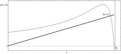
Since g(0) = r and the fact that g(x) tends to minus infinity when x tends to α/γμ₁ from the left, and l(x) is a straight line through the origin with positive slope, there is always at least one fixed point. As we will show later (Equations (6)–(8)), in case that g(x) has negative slope at the intersection the resulting fixed point is always stable. So, for now we will concentrate in the search for intersections for which g(x) intersects l(x) at a point where both functions have positive slopes, first of at least one such fixed point, and later for specific conditions for the existence of exactly such an equilibrium.

The following result provides sufficient conditions for the existence of at least one inflection point x with g(x) > 0 in the range $(0,a/\gamma {\mu }_1)$ with positive slope. In the biological context this means, under certain conditions on the learning curve β(x) and on the carrying capacity of the insect $(r/{\mu }_2>2/\gamma )$, there is an equilibrium level for the plant for which the pollinator has a maximum reaction to the deception, due for instance to effective intraspecific communication and learning.

Lemma 3.1:

If β′′(0) ≥ 0 β′(0) ≥ 0 and $r/{\mu }_2>2/\gamma$, then g has at least one inflection point, x_in, in $(0,a/\gamma {\mu }_1)$ such that $g^{\mathrm{\prime }}\left(x_{in}\right)>0$.

Proof :

We have g(0) = r. Moreover, $g^{\mathrm{\prime }}\left(0\right)=r{\beta }^{\mathrm{\prime }}\left(0\right)+{\mu }_1(\gamma r-{\mu }_2)/a$ and $g^{\mathrm{\prime \prime }}\left(0\right)=r{\beta }^{\mathrm{\prime \prime }}\left(0\right)+2{\mu }_1(\gamma {\mu }_1+a{\beta }^{\mathrm{\prime }}(0\left)\right)(\gamma r-2{\mu }_2)/a^2$. Next, making use of the hypotheses, we get $g^{\mathrm{\prime }}\left(0\right)>0$ and $g^{\mathrm{\prime \prime }}\left(0\right)>0$; i.e. g is increasing and convex when x = 0. On the other hand, we have that g(x) tends to −∞ when x tends to $\left(a/\gamma {\mu }_1\right)$ from below.

Lemma 3.1 proves the existence of an inflection point, but not its uniqueness. In what follows, unless otherwise stated, we assume that the function g(x) has a unique inflection point with positive slope, and therefore a single maximum point, x^M, as depicted in Figure 1. Later on we will comment on the possibility of g(x) having more than one inflection point. Here, we will focus on the parameter c, the measure of the damage or biological cost for the pollinator by being fooled by a deceiving plant.

Lemma 3.2:

If $g^{\mathrm{\prime }}\left(x_{in}\right)\le g\left(x_{in}\right)/x_{in}$, then $g^{\mathrm{\prime }}\left(x\right)<g\left(x\right)/x$ for all $x\in (0,x_{in})\cup (x_{in},(a/\gamma {\mu }_1\left)\right)$.

Proof :

If $x\in (0,x_{in})$, then $g^{\mathrm{\prime }}\left(x\right)<g^{\mathrm{\prime }}\left(x_{in}\right)$ by the convexity of g in the range. On the other hand, $g\left(x_{\mathrm{in}}\right)/x_{\mathrm{in}}<g\left(x\right)/x$. Note also that $g^{\mathrm{\prime }}\left(x\right)<g\left(x\right)/x$.

Analogously, for $x\in (x_{\mathrm{in}},a/\gamma {\mu }_1)$, we have $g^{\mathrm{\prime }}\left(x\right)<g^{\mathrm{\prime }}\left(x_{\mathrm{in}}\right)$ by the concavity of g. Moreover, $g\left(x_{\mathrm{in}}\right)/x_{\mathrm{in}}<g\left(x\right)/x$. Therefore, $g^{\mathrm{\prime }}\left(x\right)<g\left(x\right)/x$.

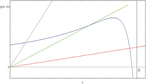
It can be seen that a consequence of Lemma 3.2 is the existence of unique equilibrium point E(x*,y*). The corresponding configuration is depicted in Figure 2.

Figure 2. When function g(x) (curve has a maximum point) satisfies the hypotheses of Lemma 3.2, we get a unique equilibrium point for different values of c (straight lines). Here, we used $\beta \left(x\right)=\beta x$.

Before proving Theorem 3.1, we consider the Jacobian matrix, J(x,y), of system (1) in order to find its eigenvalues around the equilibrium $J(x,y)=\left(\begin{array}{cc}-2{\mu }_{1}x+\frac{ay(D-x{\beta }^{\mathrm{\prime }}(x\left)\right)}{D^2}& \frac{ax(1+\beta (x\left)\right)}{D^2}\\ -\frac{cy(D-x{\beta }^{\mathrm{\prime }}(x\left)\right)}{D^2}& r-2{\mu }_{2}y-\frac{cx(1+\beta (x\left)\right)}{D^2}\end{array}\right),$ where $D=1+\beta \left(x\right)+\gamma y$.

The Jacobian matrix evaluated at E(x*,y*) is $J\left(E\right)=\left(\begin{array}{cc}{e}_1& e_2\\ e_3& e_4\end{array}\right),$ where $\begin{array}{rl}{e}_1& =-x^{\ast }\left({\mu }_1+\frac{a{y}^{\ast }{\beta }^{\mathrm{\prime }}\left(x^{\ast }\right)}{{\left[D^{\ast }\right]}^2}\right),\\ e_2& =\frac{a{x}^{\ast }(1+\beta (x^{\ast }\left)\right)}{{\left[D^{\ast }\right]}^2},\\ e_3& =-\frac{c{y}^{\ast }(D^{\ast }-x^{\ast }{\beta }^{\mathrm{\prime }}(x^{\ast }\left)\right)}{{\left[D^{\ast }\right]}^2},\\ e_4& =y^{\ast }\left(-{\mu }_3+\frac{c\gamma x^{\ast }}{{\left[D^{\ast }\right]}^2}\right),\end{array}$ and $D^{\ast }=1+\beta \left(x^{\ast }\right)+\gamma y^{\ast }.$ Note that $e_1<0<e_2$.

The eigenvalues of J(E) are given by (6) $\lambda =\frac{\tau \pm \sqrt{{\tau }^2-4\mathrm{\Delta }}}{2},$(6) where τ denotes the trace and Δ the determinant of J(E). From Equations (2) and (3), we have (7) $\mathrm{\Delta }=\frac{{\mu }_1{x}^2{(a-\gamma {\mu }_{1}x)}^2}{a^2(1+\beta (x\left)\right)}\left(\frac{g\left(x\right)}{x}-g^{\mathrm{\prime }}\left(x\right)\right)$(7) and (8) $e_4=\frac{e_2{\mu }_{1}x}{e_{1}a}\left(\frac{{\beta }^{\mathrm{\prime }}\left(x\right)(a-\gamma {\mu }_{1}x)}{a(1+\beta (x\left)\right)}g\left(x\right)-g^{\mathrm{\prime }}\left(x\right)\right).$(8)

Theorem 3.1:

Assume:

1. $g^{\mathrm{\prime }}\left(x_{in}\right)<\frac{g\left(x_{in}\right)}{x_{in}}$, and

2. $c\le {\mu }_1.$

Then system (1) has a unique equilibrium point, (x*,y*), which is globally asymptotically stable.

Proof :

From Lemma 3.2 and Equation (7), we get Δ > 0. On the other hand, we have $\tau =-{\mu }_{2}y-\frac{axy{\beta }^{\mathrm{\prime }}\left(x\right)}{{(1+\beta (x)+\gamma y)}^2}+\frac{x}{{(1+\beta (x)+\gamma y)}^2}(-{\mu }_1(1+\beta (x)+\gamma y{)}^2+c\gamma y),$ and by hypothesis $c\le {\mu }_1$. Therefore, we get τ < 0. Then, employing Equation(9), we obtain Re(λ) < 0. Hence, E(x*,y*) is locally stable.

To prove global stability, we will apply Dulac’s criterion [29], to rule out periodic orbits. Let $g(x,y)=1/xy$ and $\dot{\mathbf{\text{x}}}=\left(-{\mu }_1{x}^2+\frac{a}{1+\beta \left(x\right)+\gamma y}xy,ry-{\mu }_2{y}^2-\frac{c}{1+\beta \left(x\right)+\gamma y}xy\right),$ then $\begin{array}{rl}\mathrm{\nabla }\cdot \left(g\dot{\mathbf{\text{x}}}\right)& =\frac{\mathrm{\partial }}{\mathrm{\partial }x}\left(g\dot{x}\right)+\frac{\mathrm{\partial }}{\mathrm{\partial }y}\left(g\dot{y}\right)\\ & =\frac{\mathrm{\partial }}{\mathrm{\partial }x}\left(-\frac{{\mu }_{1}x}{y}+\frac{a}{1+\beta \left(x\right)+\gamma y}\right)+\frac{\mathrm{\partial }}{\mathrm{\partial }y}\left(\frac{r-{\mu }_{2}y}{x}-\frac{c}{1+\beta \left(x\right)+\gamma y}\right)\\ & =-\frac{{\mu }_1}{y}-\frac{a{\beta }^{\mathrm{\prime }}\left(x\right)}{{(1+\beta (x)+\gamma y)}^2}-\frac{{\mu }_2}{x}+\frac{c\gamma }{{(1+\beta (x)+\gamma y)}^2}.\end{array}$ The condition $c\le {\mu }_1$, implies $-\frac{{\mu }_1}{y}+\frac{c\gamma }{{(1+\beta (x)+\gamma y)}^2}<0.$

Theorem 3.1 assures that once considering the damping effect of learning and intraspecific communications among insects, the increase in the reproduction rate of the plants is not too big, and the biological cost for the pollinator, c, is small enough compared with the death rate of the plant, μ₁, then the system always tends to stabilize at an equilibrium level. In particular, the system is able to maintain itself, and even more, after small perturbations in the environment, it will return to its original equilibrium level x*.

The level of equilibrium for the pollinator, depends on the biological cost, c, it increases as c decreases. For smaller values of c, i.e. a lesser deceptive pollination level, the plant will attain a bigger level of occupancy, benefiting both species. Theorem 3.1 offers a possible answer to the question by Jersáková et al. [18] on the evolutionary stability of deceptive pollination.

Since condition (2) in theorem is used to exclude periodic solutions, we now turn to the possibility of oscillations appearing by increasing c beyond μ₁. As we will show, damped oscillations will first appear, and later they will turn undamped via Hopf bifurcation. Biologically this might be very dangerous for both the plant and the insect, since both will be oscillating in regions that might become too close to zero, so that any additional disturbance in the environment could cause the extinction of the plant, stopping any benefit for the insect.

The following lemma provides conditions on the eigenvalues of the linearization for the existence of oscillations via Hopf bifurcation, considering c as bifurcation parameter.

Lemma 3.3:

Assume system (1) has a unique equilibrium point, and the following hypotheses hold true:

1. ${\beta }^{\mathrm{\prime \prime }}\left(x_{in}\right)\le 0,$

2. μ₂ ≥ a.

Then, there exists c₀ such that $\lambda =\pm \sqrt{\mathrm{\Delta }}i$, where Δ > 0.

Proof :

By Lemma 3.2 always Δ > 0 in the interval $(x_{\mathrm{in}},x^M]$. From Equation (6), we have $\tau =e_1+e_4$, where e₁ < 0. For $x=x^M$, we get τ < 0 by Equation (8).

Combining Equations (4) and (5), we can rewrite τ as (9) $\begin{array}{rl}\tau & =-\frac{{\mu }_{1}x}{a(1+\beta (x\left)\right)}\left[a\right(1+\beta \left(x\right))+x{\beta }^{\mathrm{\prime }}(x\left)\right(a-\gamma {\mu }_{1}x\left)\right]\\ & +\frac{{\mu }_{1}x}{a(a-\gamma {\mu }_{1}x)}\left\{\gamma \right[r(a-\gamma {\mu }_{1}x)-{\mu }_1{\mu }_{2}x(1+\beta (x\left)\right)]-a{\mu }_2(1+\beta \left(x\right)\left)\right\}.\end{array}$(9) On the other hand, for $x=x_{\mathrm{in}}$, it holds $\begin{array}{rl}& \gamma \left[r\right(a-\gamma {\mu }_{1}x)-{\mu }_1{\mu }_{2}x(1+\beta \left(x\right)\left)\right]-a{\mu }_2(1+\beta (x\left)\right)={\mu }_{2}x(a-\gamma {\mu }_{1}x){\beta }^{\mathrm{\prime }}\left(x\right)\\ & +a{\mu }_2(1+\beta (x\left)\right)-\frac{{\beta }^{\mathrm{\prime \prime }}\left(x\right){(a-\gamma {\mu }_{1}x)}^2\left[r\right(a-\gamma {\mu }_{1}x)-2{\mu }_1{\mu }_{2}x(1+\beta \left(x\right)\left)\right]}{2{\mu }_1\left[\right(a-\gamma {\mu }_{1}x\left){\beta }^{\mathrm{\prime }}\right(x)+\gamma {\mu }_1(1+\beta \left(x\right)\left)\right]}.\end{array}$ Substituting this expression in Equation (9), we get $\begin{array}{rl}\tau & =\frac{{\mu }_1{x}_{\mathrm{in}}\left[a\right(1+\beta \left(x_{\mathrm{in}}\right))+x_{\mathrm{in}}{\beta }^{\mathrm{\prime }}(x_{\mathrm{in}}\left)\right(a-\gamma {\mu }_1{x}_{\mathrm{in}}\left)\right]}{a(1+\beta (x_{\mathrm{in}}\left)\right)(a-\gamma {\mu }_1{x}_{\mathrm{in}})}\left[{\mu }_2\right(1+\beta \left(x_{\mathrm{in}}\right))-(a-\gamma {\mu }_1{x}_{\mathrm{in}}\left)\right]\\ & -\frac{x_{\mathrm{in}}{\beta }^{\mathrm{\prime \prime }}\left(x_{\mathrm{in}}\right)(a-\gamma {\mu }_1{x}_{\mathrm{in}})\left[r\right(a-\gamma {\mu }_1{x}_{\mathrm{in}})-2{\mu }_1{\mu }_2{x}_{\mathrm{in}}(1+\beta \left(x_{\mathrm{in}}\right)\left)\right]}{2a\left[\right(a-\gamma {\mu }_1{x}_{\mathrm{in}}\left){\beta }^{\mathrm{\prime }}\right(x_{\mathrm{in}})+\gamma {\mu }_1(1+\beta \left(x_{\mathrm{in}}\right)\left)\right]}.\end{array}$ By hypothesis, ${\mu }_2\ge a$ and ${\beta }^{\mathrm{\prime \prime }}\left(x_{\mathrm{in}}\right)\le 0$, we get τ>0, at x = x_in. Continuity of τ(x) implies the existence of a $x^{c_0}$ such that $\tau \left(x^{c_0}\right)=0$. On the other hand, $x^{c_0}$ satisfies the equilibria equation cx = g(x), from this it follows the existence of a c₀ such that $c_0=g\left(x^{c_0}\right)/x^{c_0}$.

Theorem 3.2:

Assume system (1) has a unique equilibrium point, and the following hypotheses hold true:

1. ${\beta }^{\mathrm{\prime \prime }}\left(x_{in}\right)\le 0$,

2. $x^{c_0}{\beta }^{\mathrm{\prime \prime }}\left(x^{c_0}\right)+2{\beta }^{\mathrm{\prime }}\left(x^{c_0}\right)\ge 0$ and

3. ${\mu }_2\ge 2a$.

Then, system (1) has a periodic orbit around the equilibrium E(x*,y*).

Proof :

We know by Lemma 3.3 that there is a value c₀, called the bifurcation value, such that $Re\left(\lambda \right(c_0\left)\right)=0$ and $Im\left(\lambda \right(c_0\left)\right)\ne 0$. We need to prove $\text{d}Re\left(\lambda \right)\text{/d}c\ne 0$ at c = c₀.

From Equation (9), we have $\frac{\text{d}Re\left(\lambda \right)}{\text{d}c}=\frac{1}{2}\frac{\mathrm{\partial }\tau }{\mathrm{\partial }x}\frac{\text{d}x}{\text{d}c}.$ From Figure 2, clearly $\text{d}x\text{/d}c<0$. On the other hand, $\begin{array}{rl}\frac{\mathrm{\partial }\tau }{\mathrm{\partial }x}& =-\frac{{\mu }_{1}x(a-\gamma {\mu }_{1}x)}{a(1+\beta (x\left)\right)}\left(x{\beta }^{\mathrm{\prime \prime }}\right(x)+2{\beta }^{\mathrm{\prime }}(x\left)\right)\\ & -\frac{{\mu }_1{\mu }_{2}x}{a(a-\gamma {\mu }_{1}x)}\left[\right(a+\gamma {\mu }_{1}x\left){\beta }^{\mathrm{\prime }}\right(x)+\gamma {\mu }_1\beta (x\left)\right]\\ & -\frac{\gamma {\mu }_1^{2}x}{a(a-\gamma {\mu }_{1}x)}(\gamma r+{\mu }_2)+\frac{{\mu }_{1}x{\beta }^{\mathrm{\prime }}\left(x\right)}{a{(1+\beta (x\left)\right)}^2}\left[x\right(a-\gamma {\mu }_{1}x\left){\beta }^{\mathrm{\prime }}\right(x)+a(1+\beta \left(x\right)\left)\right]\\ & +\frac{\gamma {\mu }_1^{2}x}{a{(a-\gamma {\mu }_{1}x)}^2}\left\{\gamma \right[r(a-\gamma {\mu }_{1}x)-{\mu }_1{\mu }_{2}x(1+\beta (x\left)\right)]-a{\mu }_2(1+\beta \left(x\right)\left)\right\}\\ & +\frac{{\mu }_1}{a(a-\gamma {\mu }_{1}x)}\left\{\gamma \right[r(a-\gamma {\mu }_{1}x)-{\mu }_1{\mu }_{2}x(1+\beta (x\left)\right)]-a{\mu }_2(1+\beta \left(x\right)\left)\right\}\\ & -\frac{{\mu }_1}{a(1+\beta (x\left)\right)}\left[x\right(a-\gamma {\mu }_{1}x\left){\beta }^{\mathrm{\prime }}\right(x)+a(1+\beta \left(x\right)\left)\right].\end{array}$ Evaluating the expression at c = c₀, and simplifying we obtain $\begin{array}{rl}\frac{\mathrm{\partial }\tau }{\mathrm{\partial }x}\left(c_0\right)& =-\frac{{\mu }_1{x}^{c_0}(a-\gamma {\mu }_1{x}^{c_0})}{a(1+\beta (x^{c_0}\left)\right)}\left(x^{c_0}{\beta }^{\mathrm{\prime \prime }}\right(x^{c_0})+2{\beta }^{\mathrm{\prime }}(x^{c_0}\left)\right)-\frac{\gamma {\mu }_2{\left({\mu }_1{x}^{c_0}\right)}^2{\beta }^{\mathrm{\prime }}\left(x^{c_0}\right)}{a(a-\gamma {\mu }_1{x}^{c_0})}\\ & +\frac{{\mu }_1(a-\gamma {\mu }_1{x}^{c_0}){\left(x^{c_0}{\beta }^{\mathrm{\prime }}\right(x^{c_0}\left)\right)}^2}{a{(1+\beta (x^{c_0}\left)\right)}^2}-\frac{2\gamma {{\mu }_1}^2{\mu }_2{x}^{c_0}(1+\beta (x^{c_0}\left)\right)}{{(a-\gamma {\mu }_1{x}^{c_0})}^2}\\ & +\frac{{\mu }_1{x}^{c_0}{\beta }^{\mathrm{\prime }}\left(x^{c_0}\right)}{(1+\beta (x^{c_0}\left)\right)(a-\gamma {\mu }_1{x}^{c_0})}(a-\gamma {\mu }_1{x}^{c_0}-{\mu }_2(1+\beta \left(x^{c_0}\right)\left)\right).\end{array}$ Condition $e_4\left(x^{c_0}\right)>0$ implies $\frac{{\mu }_1(a-\gamma {\mu }_1{x}^{c_0}){\left(x^{c_0}{\beta }^{\mathrm{\prime }}\right(x^{c_0}\left)\right)}^2}{a{(1+\beta (x^{c_0}\left)\right)}^2}<\frac{{\mu }_1{x}^{c_0}{\beta }^{\mathrm{\prime }}\left(x^{c_0}\right)}{1+\beta \left(x^{c_0}\right)}.$ Therefore, $\begin{array}{rl}\frac{\mathrm{\partial }\tau }{\mathrm{\partial }x}\left(c_0\right)<& -\frac{{\mu }_1{x}^{c_0}(a-\gamma {\mu }_1{x}^{c_0})}{a(1+\beta (x^{c_0}\left)\right)}\left(x^{c_0}{\beta }^{\mathrm{\prime \prime }}\right(x^{c_0})+2{\beta }^{\mathrm{\prime }}(x^{c_0}\left)\right)-\frac{\gamma {\mu }_2{\left({\mu }_1{x}^{c_0}\right)}^2{\beta }^{\mathrm{\prime }}\left(x^{c_0}\right)}{a(a-\gamma {\mu }_1{x}^{c_0})}\\ & +\frac{{\mu }_1{x}^{c_0}{\beta }^{\mathrm{\prime }}\left(x^{c_0}\right)}{(1+\beta (x^{c_0}\left)\right)(a-\gamma {\mu }_1{x}^{c_0})}\left(2\right(a-\gamma {\mu }_1{x}^{c_0})-{\mu }_2(1+\beta \left(x^{c_0}\right)\left)\right)\\ & -\frac{2\gamma {{\mu }_1}^2{\mu }_2{x}^{c_0}(1+\beta (x^{c_0}\left)\right)}{{(a-\gamma {\mu }_1{x}^{c_0})}^2}.\end{array}$ By hypothesis, we have $-\frac{{\mu }_1{x}^{c_0}(a-\gamma {\mu }_1{x}^{c_0})}{a(1+\beta (x^{c_0}\left)\right)}\left(x^{c_0}{\beta }^{\mathrm{\prime \prime }}\right(x^{c_0})+2{\beta }^{\mathrm{\prime }}(x^{c_0}\left)\right)\le 0,$ and $2(a-\gamma {\mu }_1{x}^{c_0})-{\mu }_2(1+\beta (x^{c_0}\left)\right)<0$. These inequalities implies $\left(\mathrm{\partial }\tau /\mathrm{\partial }x\right)\left(c_0\right)<0.$ Hence, $\text{d}Re\left(\lambda \right)\text{/d}c\ne 0$ and c = c₀ and by the Hopf bifurcation theorem [7], we get the result.

The simulations presented in this figure, as well as the ones in Figures 4, 5 and 8, are dimensionless, but one can easily think of the units on the axes as being a proper power of 10, times the size of the population. This means, that we are especially interested in variations of the population size as a fraction of the original size. So, for instance examples (a) through (d) in Figure 3 indicate variations (increase or decrease) in population size by a factor between 2 and 3.

Figure 3. Periodic orbits for different beta functions: (a) β(x) = 0, (b) β(x) = 0.1x, (c) $\beta \left(x\right)=x^2/(4+9x^2)$, (d) $\beta \left(x\right)=x^3/(4+9x^3)$. (a) Shows that plants population achieves a significant level. (b) Shows that population level of the plant is reduced and the insect population level increases. (c, d) Shows that both populations reach significant levels.

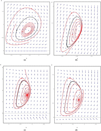
Figure 4. Equilibria points for plants x* and insects y* for different values of the parameter c. Stars represent those equilibria for which the corresponding eigenvalues of the linearization are negative, i.e. real numbers; the squares represent complex eigenvalues with negative real part and finally the plus signs represent complex eigenvalues with positive real part.

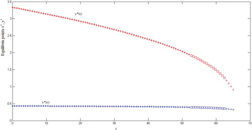
Figure 5. A typical solution of system (1) with initial condition (0.3, 0.6), for different values of c and β(x) = βx. (a) Shows that pollinator can coexist very well with the plant. (b) Shows that the insect induces a slight decrease in the initial population of the plant, and it begins to emerge a small damped oscillation after which immediately both populations recover and reach the equilibrium point. (c, d) Shows both species are forced to lower their initial size and damped oscillations become stronger. (e) Shows the solution of system (1) for which a periodic solution already appeared.

The first two conditions in Theorem 3.2 determine how the functions describing the learning process by the pollinators give rise to a Hopf bifurcation [7]. The interpretation of the third condition is that the intraspecific competition among pollinators is big enough compared to the benefit it provides to the deceptive plant. In such case both species oscillate around an equilibrium level. The mechanics for this oscillation looks like the following: an increasing number of pollinator induce an increase in the number of plants. Once the number of plant increases, the number of unrewarding visits by the pollinators also increases, which induces a reduction in the number of visits. The reduced number of pollination events finally leads to a reduction in the number of plants. Figure 3, shows simulations. In the simulations we use beta functions, they satisfy every condition of Theorem 3.2, of style: (a) β(x) = 0, (b) β(x)=βx, (c) $\beta \left(x\right)={\alpha }_1{x}^2/({\alpha }_2+{\alpha }_3{x}^2)$, (d) $\beta \left(x\right)={\delta }_1{x}^3/({\delta }_2+{\delta }_3{x}^3)$. The respective dimensions of the parameters involved are: (b) β has dimensions 1/number of plants (c) α₁ has dimensions 1/(number of plants)², α₂ is dimensionless and α₃ has dimensions 1/(number of plants)² (d) δ₁ has dimensions 1/(number of plants)³, δ₂ is dimensionless and δ₃ has dimensions 1/(number of plants)³. (a) Shows the behaviour of the solutions when there is not learning by the insects, for (b) we considered that learning by the insects is proportional to the number of plants that cheat, for (c) and (d) we are considering that at first the insect population begins to slowly learns to identify cheating plants, later the learning speed reaches its maximum and then it slowly starts decreasing until it reaches a saturation level. Simulations in (a) show the case when there is no learning by the insects: the plants population achieves a significant level compared to (b) before the periodic orbit appears. In simulation (b), there is a kind of learning (learning by insects is proportional to the number of plants that cheat) by the insects; in this case, the population level of the plant is reduced and the insect population level increases. Simulations (c) and (d) shows the orbit periodic when the function beta is sigmoidal, in these cases, both populations reach significant levels. In general, the dynamic behaviour strongly depends on the form of learning by the insects (β(x)) and the biological cost to the pollinator (c).

Combining the interpretation of Theorems 3.1 and 3.2, we see that for low levels of deception both species coexist and stabilize at the equilibrium but, for bigger values of c, i.e. a bigger biological cost for the pollinator, the systems starts to oscillate. This oscillation increases in amplitude, making it possible that the plant as well as the pollinator population approach very low levels. Any addition perturbation could make them go extinct even before the appearance of sustained oscillations. In such case, it is of interest to know how big these oscillations can get. Here, we present some simulations for a specific function to show that that risk is important.

We set the following values for the parameters: ${\mu }_1=2,a=2,r=10,{\mu }_2=3,\gamma =2,$ and the function β(x) = 0.1x. We calculated equilibrium points of both species for different values of c. For each c, Figure 4 shows the plant population, x*, and insect population y*, both at equilibrium. Observe that the insect’s population at equilibrium decreases fast, while the plant population remains almost constant.

In Figure 4 we see that for small values of c equilibria are locally stable (as predicted by Theorem 3.1). The value of c can be increased considerably before oscillations appear, allowing the plant population to be maintained by the pollinators. Later (as predicted by Theorem 3.2) eigenvalues turn complex giving rise to damped and later sustained oscillations.

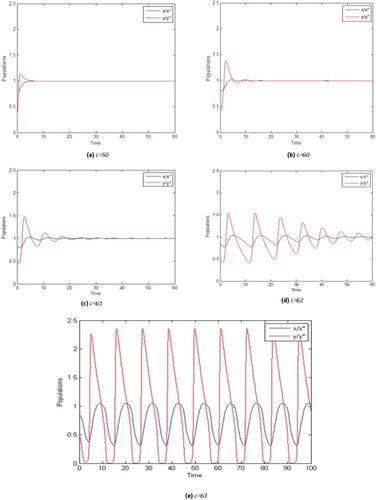
In Figure 5, we show a variety of behaviours of system (1) for solutions with initial condition (0.3,0.6) for many values of c. x and y were normalized for the equilibria point x* and y* to be equal to 1. Figure 5(a) for instance shows the behaviour of the solutions with c = 50. In this case both populations increase their initial size until they reach the equilibrium level. In this case pollinators need not reduce their initial population. With this level of deception, pollinator can coexist very well with the plant.

When the value of c = 60, Figure 5(b) shows that the insect induces a slight decrease in the initial population of the plant, and it begins to emerge a small damped oscillation after which immediately both populations recover and reach the equilibrium point. With c = 61, Figure 5(c) shows both species are forced to lower their initial size and damped oscillations become stronger until they can almost persist as it is shown in Figure 5(d) with c = 62. Biologically, this mathematical behaviour indicates that the damage caused by the plant´s adaptation, even though it is in no way sensed by the plant, has a high cost for the pollinator. The most critical case arises when c = 63, Figure 5(e) shows the solution of system (1) for which a periodic solution already appeared. Notice that the amplitude of the oscillation is very high, and the solutions do not tend to nontrivial equilibria points any more. Biologically, this behaviour is very dangerous because insect population reaches very low levels; which means that any external disturbance, for example, environmental disaster, can cause extinction of both species. In summary, after observing the behaviour of solutions with initial condition (0.3,0.6) for different values of c, we can say that for ‘small’ deception levels the plant-insect system can coexist, but for increasing values of the parameter c, both populations become extinct.

Since the appearance of oscillation is not desirable for the species, we now analyse for special cases how big the parameter c has to be in order for the oscillations to start, and eventually become sustained. The graph in Figure 6 shows such behaviour for β(x) being a straight line of slope δ. We are especially interested in the onset of oscillations and in the moment they become sustained.

Figure 6. c as a function of the parameter δ, for the special case β(x) = δx. The stars represent the value of c for which oscillations start, and the small circles represent the onset of periodic solutions. This graph shows how an increase in the cost of deception, c, requires a quicker learning by the insect, δ, in order to balance the damage and allow coexistence of both species.

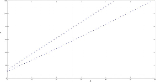
We take β(x) = δx, Figure 6 shows the behaviour of c as a function of the parameter δ. Here, c represents the biological cost to the pollinator and δ represents the reaction to the deception. If δ is big then the visit of pollinators is reduced rapidly. The stars represent the value of c for which oscillations start, and the small circles represent the onset of periodic solutions. Figure 6 shows how an increase in the cost of deception, c, requires a quicker learning by the insect, δ, in order to balance the damage and allow coexistence of both species. This might suggest an evolutive advantage if plants were able to ‘sense’ the reaction capacity of the insects in order to avoid going beyond their learning threshold. In fact, any mechanism allowing the plant to evaluate the damage it produces could lead to a maximization of the benefit for the plant. The authors do not know of any report that plant sense the damage they inflict upon the insects, but it could be interesting to study the possibility. This could for instance be a strategy followed by some orchids in using sexual deception as described in [26].

Even though we imposed some strong conditions on the function g(x) in order to show Theorems 3.1 and 3.2, the results presented can be generalized to a bigger number of steady states. In what follows, we give conditions for the existence of multiple equilibria. Figure 7 shows such an example; each straight line shows a different case and the possibility of one or multiple steady states.

Figure 7. When the function g(x) satisfies conditions in Lemma 3.4, there are values of c, the slope of the straight line l(x), for which multiple steady-state coexist. Here we used β(x) = βx.

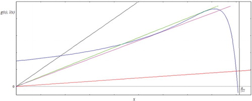
Figure 8. Periodic orbits for different beta functions: (a) β(x) = 0, in this case, the plants population achieves a significant level; (b) β(x) = 0.1x, in this case, the population level of the plant is reduced and the insect population level increases; (c) $\beta \left(x\right)=x^2/(4+9x^2)$ and (d) $\beta \left(x\right)=x^3/(4+9x^3)$ in these cases both populations reach significant levels.

In the next lemma, we stated the existence of a tangency point between g and the straight line with slope c closest to x^M.

Lemma 3.4:

If $g^{\mathrm{\prime }}\left(x_{in}\right)>g\left(x_{in}\right)/x_{in}$, then the equation $g^{\mathrm{\prime }}\left(x\right)=g\left(x\right)/x$ has exactly two solutions, $x^{T_1}\in (0,x_{in})$ and $x^{T_2}\in (x_{in},x^M)$.

Proof :

Let $f\left(x\right)=\left(g\right(x\left)/x\right)-g^{\mathrm{\prime }}\left(x\right)$, then by hypothesis $f\left(x_{\mathrm{in}}\right)<0$. On the other hand, we have that $\underset{x\to 0^{+}}{lim}{g}^{\mathrm{\prime }}\left(x\right)$ is finite, this imply that f(x) tends to ∞ when x tends to 0 from over. Moreover, by continuity of f(x), we have the existence of a $x^{T_1}$ in (0,x_in) such that $f\left(x^{T_1}\right)=0$. And by convexity of g(x) in the interval (0,x_in), we have the uniqueness.

On the other hand, clearly f > 0 at x = x^M. Hence, we have the existence of a $x^{T_2}$ in $(x_{\mathrm{in}},x^M)$, such that $f\left(x^{T_2}\right)=0$. Now, by concavity of g(x) in $(x_{\mathrm{in}},x^M)$, we have the uniqueness of $x^{T_2}$.

When we vary the parameter c, Lemma 3.4 states the existence of multiple equilibria of the system as shown in Figure 7.

Under the hypothesis of Lemma 3.4, the following theorem shows the stability of the equilibrium points in the range of $(0,a/\gamma {\mu }_1)$.

Theorem 3.3:

Let $g^{\mathrm{\prime }}\left(x_{in}\right)>g\left(x_{in}\right)/x_{in}$ and E(x*,y*) an equilibria point of system (1):

1. If $x^{\ast }\in (x^{T_1},x^{T_2})$, then E(x*,y*) is a saddle point.

2. If $x^{\ast }=x^{T_1}$($x^{\ast }=x^{T_2}$) and $e_4\le 0$, then ${\lambda }_1<0$ y ${\lambda }_2=0$.

3. If $x^{\ast }\notin [x^{T_1},x^{T_2}]$ and $e_4\le 0$, then E(x*,y*) is stable. Furthermore, provided that $x^{\ast }\in [x^M,\frac{a}{\gamma {\mu }_1})$ the equilibria E(x*,y*) is stable.

Proof :

1. If $x^{\ast }\in (x^{T_1},x^{T_2})$, then $g\left(x^{\ast }\right)/x^{\ast }<g^{\mathrm{\prime }}\left(x^{\ast }\right)$, implying $\mathrm{\Delta }<0$.

2. At the tangent point, $\mathrm{\Delta }=0$. Condition $e_4\le 0$, implies ${\lambda }_1=\tau <0$ and ${\lambda }_2=0$.

3. If $x^{\ast }\notin [x^{T_1},x^{T_2}]$, we have $g\left(x^{\ast }\right)/x^{\ast }>g^{\mathrm{\prime }}\left(x^{\ast }\right)$, this inequality implies $\mathrm{\Delta }>0$. From the condition $e_4\le 0$, we get $Re\left(\lambda \right)<0.$ Furthermore, $e_4=\frac{e_2{\mu }_1{x}^{\ast }}{e_{1}a}\left(\frac{{\beta }^{\mathrm{\prime }}\left(x^{\ast }\right)(a-\gamma {\mu }_1{x}^{\ast })}{a(1+\beta (x^{\ast }\left)\right)}g\left(x^{\ast }\right)-g^{\mathrm{\prime }}\left(x^{\ast }\right)\right)<0,$

provided that $x^{\ast }\in [x^M,a/\gamma {\mu }_1)$.

The following lemma helps us to prove the existence of a periodic orbit under some conditions.

Lemma 3.5:

Assume $g^{\mathrm{\prime }}\left(x_{in}\right)>g\left(x_{in}\right)/x_{in}$, ${\mu }_2\ge 2a$ and $\left(x^{T_2}{\beta }^{\mathrm{\prime }}\right(x^{T_2}\left)/\right(1+\beta \left(x^{T_2}\right)\left)\right)<1$, then there exists c₀ such that $\lambda =\pm \sqrt{\mathrm{\Delta }}i$, where $\mathrm{\Delta }>0$.

Proof :

At $x=x^M$ by Equation (8), we have $Re\left(\lambda \right(x^M\left)\right)<0.$ On the other hand, the equation $g\left(x^{T_2}\right)/x^{T_2}=g^{\mathrm{\prime }}\left(x^{T_2}\right)$, implies $\begin{array}{rl}& {\mu }_1{x}^{T_2}\left\{\gamma \right[r(a-\gamma {\mu }_1{x}^{T_2})-{\mu }_1{\mu }_2{x}^{T_2}(1+\beta (x^{T_2}\left)\right)]-a{\mu }_2(1+\beta \left(x^{T_2}\right)\left)\right\}\\ & =\frac{x^{T_2}(a-\gamma {\mu }_1{x}^{T_2}){\beta }^{\mathrm{\prime }}\left(x^{T_2}\right)}{1+\beta \left(x^{T_2}\right)}\left\{{\mu }_1{\mu }_2{x}^{T_2}\right(1+\beta \left(x^{T_2}\right))-[r(a-\gamma {\mu }_1{x}^{T_2})\\ & -{\mu }_1{\mu }_2{x}^{T_2}(1+\beta (x^{T_2}\left)\right)\left]\right\}+(a-\gamma {\mu }_1{x}^{T_2})\left[r\right(a-\gamma {\mu }_1{x}^{T_2})\\ & -{\mu }_1{\mu }_2{x}^{T_2}(1+\beta (x^{T_2}\left)\right)].\end{array}$ Substituting this expression in e₄, we get $\begin{array}{rl}{e}_4& =\frac{x^{T_2}{\beta }^{\mathrm{\prime }}\left(x^{T_2}\right)}{a(1+\beta (x^{T_2}\left)\right)}\left\{{\mu }_1{\mu }_2{x}^{T_2}\right(1+\beta \left(x^{T_2}\right))-[r(a-\gamma {\mu }_1{x}^{T_2})-{\mu }_1{\mu }_2{x}^{T_2}(1+\beta (x^{T_2}\left)\right)\left]\right\}\\ & +\frac{1}{a}\left[r\right(a-\gamma {\mu }_1{x}^{T_2})-{\mu }_1{\mu }_2{x}^{T_2}(1+\beta \left(x^{T_2}\right)\left)\right].\end{array}$ Then, adding e₁ to e₄, we get $\begin{array}{rl}\tau \left(x^{T_2}\right)& =\frac{1}{a}\left(1-\frac{x^{T_2}{\beta }^{\mathrm{\prime }}\left(x^{T_2}\right)}{1+\beta \left(x^{T_2}\right)}\right)\left[r\right(a-\gamma {\mu }_1{x}^{T_2})-{\mu }_1{\mu }_2{x}^{T_2}(1+\beta \left(x^{T_2}\right))-a{\mu }_1{x}^{T_2}]\\ & +\frac{{\mu }_1{\left(x^{T_2}\right)}^2{\beta }^{\mathrm{\prime }}\left(x^{T_2}\right)}{a(1+\beta (x^{T_2}\left)\right)}\left[{\mu }_2\right(1+\beta \left(x^{T_2}\right))-a-(a-\gamma {\mu }_1{x}^{T_2}\left)\right].\end{array}$ By the assumptions, $\tau \left(x^{T_2}\right)>0.$ Hence, by continuity of τ(x), we conclude the existence of a $x^{c_0}$ such that $\tau \left(x^{c_0}\right)=0$. On the other hand, $x^{c_0}$ satisfies the equilibria equation cx = g(x). This equation implies the existence of c₀ such that $c_0=g\left(x^{c_0}\right)/x^{c_0}$.

Theorem 3.4:

Assume the following conditions hold true:

1. $\frac{g\left(x_{in}\right)}{x_{in}}<g^{\mathrm{\prime }}\left(x_{in}\right)$,

2. $\frac{x^{T_2}{\beta }^{\mathrm{\prime }}\left(x^{T_2}\right)}{1+\beta \left(x^{T_2}\right)}\le 1$,

3. $x^{c_0}{\beta }^{\mathrm{\prime \prime }}\left(x^{c_0}\right)+2{\beta }^{\mathrm{\prime }}\left(x^{c_0}\right)\ge 0$, and

4. ${\mu }_2\ge 2a$.

Then, there is a periodic orbit around the equilibrium E(x*,y*) and $x^{T_2}<x^{\ast }<x^M$.

Proof :

We know by Lemma 3.5 that there is a value c₀, such that $Re\left(\lambda \right(c_0\left)\right)=0$ and $Im\left(\lambda \right(c_0\left)\right)\ne 0$. The proof of the condition $\text{d}Re\left(\lambda \right)\text{/d}c\ne 0$ at c = c₀; is analogous to that of Theorem 3.2.

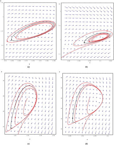
The main biologically relevant difference between this case and Theorem 3.2 is the fact that the oscillation assured in Theorem 3.4 can disappear under some disturbances. Figure 8 shows cases for which an unstable periodic solution appears for β(x).

Results obtained in this work were made considering that the function g has a unique inflection point. But, depending on the selection of the parameters and function β one can obtain a corresponding function g with multiple inflection points, in such case the system (1) can have multiple equilibria points and even multiple periodic orbits. Repeating the local analysis for each of the stable fixed points, one can show that some parameters make each point turn into an unstable one, giving rise to Hopf bifurcation. The precise conditions for that to occur are given by Lemma 3.1. The same line of thought would prove analogous generalizations in the case of multiple inflection points.

For an example of a function β that causes g to have multiple inflection points consider $\beta \left(x\right)=\frac{x^2}{1+x^2},$ with parameters, a = 100, r = 3000, µ₂ = 300, µ₁ = 2, γ = 1, the function g(x) has the following inflection points: x₁ = 0.5840, x₂ = 8.1737 and x₃ = 24.9799.

The biological interpretation of this kind of behaviour is that the learning process starts slowly, later it increases more rapidly, and finally, for big numbers of the insect population, it levels down again.

Because of its biological significance and corresponding consequences, the main purpose of this work was to show the conditions under which oscillations and periodic solutions arise. But this does not rule out that the system (1) can have more complex behaviours such as the existence of multiple periodic orbits.

4. Discussion

The main purpose of this work was to present and analyse a mathematical model for understanding the complex interaction between deception by plants and learning by insects. In the specific model, the deceptive pollination is obligatory for the plant population and the pollinators are able to learn from unrewarding visits, reducing the number of pollinated plants by reducing visiting. Learning has been observed in insects pollinating deceiving orchids [11,14,15,25]. This interactions, deception and learning, are modelled by the parameter c and function β in system (1).

The main results outlined in the theorems describe the possible behaviours depending on the parameter c, which represents the biological cost for the pollinator being deceived. At low levels of deceptiveness, the pollinators sustain a reduction on the numbers of individuals at equilibrium. The equilibrium is a global attractor, which means that for almost any initial condition or disturbances, the system tends to return to the equilibrium level. In particular, even though the plants depend exclusively on the deceptive pollination, it is always possible for the plant to parasitize the pollinator population via deception, and even obtaining a maximum benefit avoiding collapse of the system. In particular, we believe that Theorems 3.1 and 3.2, for small values of c shed important light on the question, IS FLORAL DECEPTION EVOLUTIONARILY STABLE?, stated by Jersáková et al. [18] and give a reasonable mechanism for sexual deceit as an efficient pollination facilitator in orchids.

For bigger biological cost for the insects, (i.e. bigger values of c), the system start oscillating around the equilibrium level making it dangerous for both species, since they approach very low levels, making them prone to extinction due to any additional environmental element. Numerical simulations show that this danger appears long before the periodic solutions occur.

For an increasing level of deceptiveness, that equilibrium can turn unstable, giving way to a sustained oscillation around the equilibrium. The oscillations, once they appear, turn to be stable, attracting any other solution.

For even greater values of c, the biological cost of being fooled, the oscillations turn wilder, allowing the number of individuals to increase above the equilibrium, but also reducing the numbers far below the equilibrium. As c is so bigger, against any additional disturbance, the insects are more strongly affected and more likely to go extinct first, and in consequence to extinction of both species involved.

From the evolutionary perspective one should expect to find species of plants that deceive, as it is actually the case, but only if the biological cost for the pollinator remains limited. Otherwise, both species involved would disappear in the evolutionary race. Of course, this extinction of both species has also to do with learning insects which is measured by the function β; that is to say, the insect can prevent the collapse of its population, if it could detect the deception of the plants rapidly enough and consequently decrease the cost of being deceived. Although the quantitative measurement of the learning rate (β) is difficult to perform, some authors have done research in this field, for example, Dukas and Bernays [5] performed an experiment about the role of learning in acquiring an optimally balanced diet in grasshoppers and they showed that the behavioural differences between the treatments translated into a 20% higher growth rate in the learning grasshoppers compared with the random grasshoppers. Another quantitative study on learning is given in the paper by Leadbeater and Chittka [20] here, the authors used a quantitative analysis of learning in a forage task to illustrate that the attraction of bumble bees (Bombus terrestris) to those particular inflorescences where other bees are already foraging can lead bees to learn more quickly which flower species are rewarding if they forage in the company of experienced conspecifics.

It would be of special interest to consider how a bigger value of c would accelerate the learning process in insects. One would expect that a small cost, like missed feeding opportunity would induce a much smaller learning than a costly sperm wastage incurred by the insect if actual copulation takes place in setting with strong intraspecific competition.

During recent years massive local extinctions have been observed, for instance, the local honeybee populations have collapsed in several regions and countries [2], making it very important to understand how the regular dynamics might work and which potential dangers are hidden in the intrinsic dynamics of the system. The authors do not know of specific oscillations of the population shortly before disappearing, but if that is a plausible mechanism for extinction, we should be aware of it.

Often the plant and pollinator distributions do not show much overlap [23]. In these cases, the pollinator population may not experience much coevolution as only a very small part of the population encounters the deceptive plants and experiments costs. This is also likely to affect evolutionary outcomes. Considering the generation times of the plants and the insects will likely also have large impacts on evolutionary outcomes. Insects often have short annual or seasonal generation times, but orchids may live for decades. This means that if pollinator populations become dangerously low, it will not immediately affect the plants negatively, and plants may be able to easily persist during insect population size oscillations until the insect populations recovers; this is possible because we assumed in our model that the insect feeds on alternative plants with flowers. But if insect population’s sizes are plummeting, the plants may initially remain abundant and therefore continue to drive the insect populations further down. This may in fact then hasten the local extinction of pollinators, and eventually of the plants as well, as our model predicts. These hypotheses posed depend on how large is the population of plants that offer reward versus those who cheat and other factors; but this topic would remain pending for future work.

Also, as future work would be of interest to propose different functions beta and designing experiments to actually measure the learning process and its effect on the change in strategy by the deceiving plant. Is there a better function for the insect or for the plant? Does the same plant present different reproductive strategies depending on the insects it relies on for pollination? What about different strategies for different environmental conditions? Has evolution changed the learning response by the insects and changed the strategy of the plants accordingly? It is very likely that functional responses have evolved in different directions and it is our challenge to try to understand them, especially in a setting when human influences are increasingly affecting natural ecosystems.

Acknowledgements

We thank an anonymous reviewer for insightful comments.

Disclosure statement

No potential conflict of interest was reported by the authors.

References

- D.P. Abrol, Pollination biology, Springer, Dordrecht, 2012. doi: 10.1007/978-94-007-1942-2 .
- J. Biesmeijer, S. Roberts, and M. Reemer, Parallel declines in pollinators and insect-pollinated plants in Britain and the Netherlands, Science 313 (2006), pp. 351–354. doi: 10.1126/science.1127863
- D. Clarke, H. Whitney, G.P. Sutton, and D. Robert, Detection and learning of floral electric fields by bumblebees, Science. 340 (2013), pp. 66–69. doi: 10.1126/science.1230883.
- A. Dafni, Mimicry and deception in pollination, Annu. Rev. Ecol. Syst. 15 (1984), pp. 259–278. doi: 10.1146/annurev.es.15.110184.001355
- R. Dukas and E. Bernays, Learning improves growth rate in grasshoppers, Proc. Natl. Acad. Sci. USA 97 (2000), pp. 2637–2640. doi: 10.1073/pnas.050461497
- R. Dukas and L.A. Real, Learning constraints and floral choice behaviour in bumble bees, Anim. Behav. 46 (1993), pp. 637–644. doi: 10.1006/anbe.1993.1240.
- L. Edelstein-Keshet, Mathematical Models in Biology, Society for Industrial and Applied Mathematics, Philadelphia, 1988.
- A. Edwards and A. Yool, The role of higher predation in plankton population models, J. Plankton Res. 22 (2000), pp. 1085–1112. doi: 10.1093/plankt/22.6.1085
- A. Edwards and J. Brindley, Oscillatory behaviour in a three-component plankton population model, Dyn. Stab. Syst. 11 (1996), pp. 347–370. doi: 10.1080/02681119608806231
- J. Ferdy, F. Austerlitz, J. Moret, P. Gouyon, and B. Godelle, Pollinator-induced density dependence in deceptive species, Oikos 87 (1999), pp. 549–560. doi: 10.2307/3546819
- J.B. Ferdy, P.H. Gouyon, J. Moret, and B. Godelle, Pollinator behavior and deceptive pollination: learning process and floral evolution, Am. Nat. 152 (1998), pp. 696–705. doi: 10.1086/286200.
- A. Gaskett and C. Winnick, Orchid sexual deceit provokes ejaculation, Am. Nat. 171 (2008), pp. E206–E212. doi: 10.1086/587532
- A. Gumbert, Color choices by bumble bees (Bombus terrestris): Innate preferences and generalization after learning, Behav. Ecol. Sociobiol. 48 (2000), pp. 36–43. doi:10.1007/s002650000213. doi: 10.1007/s002650000213
- A.I. Internicola, P.A. Page, G. Bernasconi, and L.D.B. Gigord, Competition for pollinator visitation between deceptive and rewarding artificial inflorescences: An experimental test of the effects of floral colour similarity and spatial mingling, Funct. Ecol. 21 (2007), pp. 864–872. doi: 10.1111/j.1365-2435.2007.01303.x.
- M.L. de Jager and A.G. Ellis, Costs of deception and learned resistance in deceptive interactions, Proc. R. Soc. B. 281 (2014), pp. 20132861. doi: 10.1098/rspb.2013.2861.
- M. de Jager, E. Newman, G. Theron, P. Botha, M. Barton, and B. Anderson, Pollinators can prefer rewarding models to mimics: Consequences for the assumptions of Batesian floral mimicry, Plant Syst. Evol. 302 (2016), pp. 409–418. doi: 10.1007/s00606-015-1276-0.
- S. Jang and J. Baglama, Nutrient-plankton models with nutrient recycling, Comput. Math. Appl. 49 (2005), pp. 375–387. doi: 10.1016/j.camwa.2004.03.013
- J. Jersáková, S.D. Johnson, and P. Kindlmann, Mechanisms and evolution of deceptive pollination in orchids, Biol. Rev. 81 (2006), pp. 219–235. doi: 10.1017/S1464793105006986.
- C.A. Kearns, D.W. Inouye, and N.M. Waser, Endangered mutualisms: The conservation of plant–pollinator interactions, Annu. Rev. Ecol. Syst. 29 (1998), pp. 83–112. doi: 10.1146/annurev.ecolsys.29.1.83
- E. Leadbeater and L. Chittka, The dynamics of social learning in an insect model, the bumblebee (Bombus terrestris), Behav. Ecol. Sociobiol. 61 (2007), pp. 1789–1796. doi: 10.1007/s00265-007-0412-4
- K. Lunau and E.J. Maier, Innate colour preferences of flower visitors, J. Comp. Physiol. A 177 (1995), pp. 1–19. doi: 10.1007/BF00243394
- R. Mitchell, R. Irwin, R. Flanagan, and J. Karron, Ecology and evolution of plant–pollinator interactions, Ann. Bot. 103 (2009), pp. 1355–1363. doi: 10.1093/aob/mcp122
- R. Peakall, L. Jones, C.C. Bower, and B.G. Mackey, Bioclimatic assessment of the geographic and climatic limits to hybridisation in a sexually deceptive orchid system, Aust. J. Bot. 50 (2002), pp. 21–30. doi: 10.1071/BT01021.
- C. Salzmann, A. Nardella, S. Cozzolino, and F.P. Schiestl, Variability in floral scent in rewarding and deceptive orchids: the signature of pollinator-imposed selection? Ann. Bot. 100 (2007), pp. 757–765. doi: 10.1093/aob/mcm161
- F.P. Schiestl, On the success of a swindle: pollination by deception in orchids, Naturwissenschaften 92 (2005), pp. 255–264. doi: 10.1007/s00114-005-0636-y.
- G. Scopece, S. Cozzolino, S.D.D. Johnson, and F.P.P. Schiestl, Pollination efficiency and the evolution of specialized deceptive pollination systems, Am. Nat. 175 (2010), pp. 98–105. doi: 10.1086/648555.
- A. Smithson and M. MacNair, Negative frequency-dependent selection by pollinators on artificial flowers without rewards, Evolution 51 (1997), pp. 715–723. doi: 10.1111/j.1558-5646.1997.tb03655.x
- C. Sprengel, Das entdeckte Geheimnis der Natur im Bau und in der Befruchtung der Blumen, 1793.
- S. Strogatz, Nonlinear Dynamics and Chaos: with Applications to Physics, Biology, Chemistry and Engineering, Westview Press, Cambridge, MA, 2001.
- R. Tremblay, Trends in the pollination ecology of the Orchidaceae: Evolution and systematics, Can. J. Bot. 70 (1992), pp. 642–650. doi: 10.1139/b92-083
- B. Wong and F. Schiestl, How an orchid harms its pollinator, Proc. R. Soc. B Biol. Sci. 269 (2002), pp. 1529–1532. doi: 10.1098/rspb.2002.2052