Bifurcation analysis and chaos control for a plant–herbivore model with weak predator functional response

Abstract

The interaction between plants and herbivores is one of the most fundamental processes in ecology. Discrete-time models are frequently used for describing the dynamics of plants and herbivores interaction with non-overlapping generations, such that a new generation replaces the old at regular time intervals. Keeping in view the interaction of the apple twig borer and the grape vine, the qualitative behaviour of a discrete-time plant–herbivore model is investigated with weak predator functional response. The topological classification of equilibria is investigated. It is proved that the boundary equilibrium undergoes transcritical bifurcation, whereas unique positive steady-state of discrete-time plant–herbivore model undergoes Neimark–Sacker bifurcation. Numerical simulation is provided to strengthen our theoretical discussion.

Keywords:

• Plant–herbivore model
• stability
• transcritical bifurcation
• Neimark–Sacker bifurcation
• chaos control

2010 AMS Mathematics Subject Classifications:

• 39A30
• 40A05
• 92D25
• 92C50

1. Introduction

In mathematical biology, plant–herbivore models are basically modifications of prey–predator models [8]. The interaction between plants and herbivores has been investigated by many researchers both in differential and difference equations. Kartal [31] investigated the dynamical behaviour of a plant–herbivore model including both differential and difference equations. In [30] Kang et al. discussed bistability, bifurcation and chaos control in a discrete-time plant–herbivore model. In [38] Liu et al. investigated stability, limit cycle, Neimark–Sacker bifurcations and homoclinic bifurcation for a plant–herbivore model with toxin-determined functional response. Li et al. [37] discussed period-doubling and Neimark–Sacker bifurcations for a plant–herbivore model incorporating plant toxicity in the functional response of plant–herbivore interactions. Similarly, for some other discussions related to qualitative behaviour of plant–herbivore models, the interested reader is referred to [2,10,21,25–27,29,33,45,47,52] and references are therein.

Taking into account the interaction of the apple twig borer and the grape vine [3], a mathematical model for plant–herbivore interaction based on weak predator functional response is given by (1) $\begin{array}{rl}{x}_{n+1}& =\frac{x_n}{\alpha (1+y_n^2)+\beta x_n},\\ y_{n+1}& =\gamma y_n(1+x_n),\end{array}$(1) where $x_n$ and $y_n$ are population densities for grape vine and apple twig borer, respectively. Moreover, α, β and γ are positive parameters. For some earlier investigations related to model (1(1) $\begin{array}{rl}{x}_{n+1}& =\frac{x_n}{\alpha (1+y_n^2)+\beta x_n},\\ y_{n+1}& =\gamma y_n(1+x_n),\end{array}$(1) ), we refer to [4–7,34,35]. Moreover, taking into account strong predator functional response, Din [12] discussed global stability of system (1(1) $\begin{array}{rl}{x}_{n+1}& =\frac{x_n}{\alpha (1+y_n^2)+\beta x_n},\\ y_{n+1}& =\gamma y_n(1+x_n),\end{array}$(1) ), and Khan et al. [32] investigated Neimark–Sacker bifurcation for system (1(1) $\begin{array}{rl}{x}_{n+1}& =\frac{x_n}{\alpha (1+y_n^2)+\beta x_n},\\ y_{n+1}& =\gamma y_n(1+x_n),\end{array}$(1) ) with strong predator functional response.

The main findings of this paper are summarized as follows:

• Existence of equilibria and their stability analysis is investigated.

• It is proved that model (1(1) $\begin{array}{rl}{x}_{n+1}& =\frac{x_n}{\alpha (1+y_n^2)+\beta x_n},\\ y_{n+1}& =\gamma y_n(1+x_n),\end{array}$(1) ) undergoes transcritical bifurcation at its boundary equilibrium by implementing bifurcation theory of normal forms and centre manifold theorem.

• Direction and existence criteria for Neimark–Sacker bifurcation are investigated at positive steady-state of plant–herbivore model (1(1) $\begin{array}{rl}{x}_{n+1}& =\frac{x_n}{\alpha (1+y_n^2)+\beta x_n},\\ y_{n+1}& =\gamma y_n(1+x_n),\end{array}$(1) ).

• Pole-placement and hybrid control methods are implemented in order to discuss chaos control in system (1(1) $\begin{array}{rl}{x}_{n+1}& =\frac{x_n}{\alpha (1+y_n^2)+\beta x_n},\\ y_{n+1}& =\gamma y_n(1+x_n),\end{array}$(1) ).

Moreover, in Section 2 the existence of steady-states and their local asymptotic behaviour is analysed. Section 3 is dedicated to investigate transcritical bifurcation about boundary steady-state of system (1(1) $\begin{array}{rl}{x}_{n+1}& =\frac{x_n}{\alpha (1+y_n^2)+\beta x_n},\\ y_{n+1}& =\gamma y_n(1+x_n),\end{array}$(1) ). In Section 4, we discuss Neimark–Sacker bifurcation at positive steady-state of model (1(1) $\begin{array}{rl}{x}_{n+1}& =\frac{x_n}{\alpha (1+y_n^2)+\beta x_n},\\ y_{n+1}& =\gamma y_n(1+x_n),\end{array}$(1) ). We study pole-placement chaos control and hybrid control strategies in Section 5. Finally, in Section 6, numerical simulations are carried out to authenticate the theoretical discussion.

2. Existence of equilibria and stability

In this section, first we investigate fixed points for system (1(1) $\begin{array}{rl}{x}_{n+1}& =\frac{x_n}{\alpha (1+y_n^2)+\beta x_n},\\ y_{n+1}& =\gamma y_n(1+x_n),\end{array}$(1) ). For this, these fixed points must solve the following algebraic system: (2) $x=\frac{x}{\alpha (1+y^2)+\beta x},y=\gamma (1+x)y.$(2) Simple computation yields the following steady-states for the plant–herbivore model (1(1) $\begin{array}{rl}{x}_{n+1}& =\frac{x_n}{\alpha (1+y_n^2)+\beta x_n},\\ y_{n+1}& =\gamma y_n(1+x_n),\end{array}$(1) ): $P_0=(0,0),P_1=(\frac{1-\alpha }{\beta },0),P_{\ast }=(\frac{1-\gamma }{\gamma },\sqrt{\frac{\gamma (1+\beta )-(\alpha \gamma +\beta )}{\alpha \gamma }}).$ 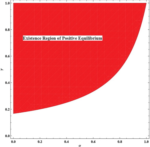Assume that $0<\alpha <1,\beta >0,\beta /(1-\alpha +\beta )<\gamma <1$, then $P_{\ast }$ is unique positive equilibrium point of the system (1(1) $\begin{array}{rl}{x}_{n+1}& =\frac{x_n}{\alpha (1+y_n^2)+\beta x_n},\\ y_{n+1}& =\gamma y_n(1+x_n),\end{array}$(1) ). For $\beta =0.2$, the region in $\alpha \gamma$-plane where inequalities $0<\alpha <1,\beta /(1-\alpha +\beta )<\gamma <1$ are satisfied is depicted in Figure 1 by red shaded region. In order to see the dynamical behaviour of system (1(1) $\begin{array}{rl}{x}_{n+1}& =\frac{x_n}{\alpha (1+y_n^2)+\beta x_n},\\ y_{n+1}& =\gamma y_n(1+x_n),\end{array}$(1) ) at equilibria, we first compute Jacobian matrix of system (1(1) $\begin{array}{rl}{x}_{n+1}& =\frac{x_n}{\alpha (1+y_n^2)+\beta x_n},\\ y_{n+1}& =\gamma y_n(1+x_n),\end{array}$(1) ) at $(x,y)$ as follows: (3) $J(x,y):=\left(\begin{array}{cc}{\displaystyle \frac{\alpha (1+y^2)}{{(\alpha (1+y^2)+\beta x)}^2}}& -{\displaystyle \frac{2\alpha xy}{{(\alpha (1+y^2)+\beta x)}^2}}\\ \gamma y& \gamma (1+x)\end{array}\right).$(3) Then, at $(x,y)=(0,0)$ the Jacobian matrix $J(x,y)$ given in (3(3) $J(x,y):=\left(\begin{array}{cc}{\displaystyle \frac{\alpha (1+y^2)}{{(\alpha (1+y^2)+\beta x)}^2}}& -{\displaystyle \frac{2\alpha xy}{{(\alpha (1+y^2)+\beta x)}^2}}\\ \gamma y& \gamma (1+x)\end{array}\right).$(3) ) reduces to $J(0,0):=\left(\begin{array}{ccc}{\displaystyle \frac{1}{\alpha }}& 00& \gamma \end{array}\right).$ Then topological classification of $P_0$ is given as follows:

• $P_0$ is a sink if and only if $\alpha >1$ and $0<\gamma <1$.

• $P_0$ is a saddle point if and only if $0<\alpha <1$ and $0<\gamma <1$, or $\alpha >1$ and $\gamma >1$.

• $P_0$ is a source if and only if $0<\alpha <1$ and $\gamma >1$.

• $P_0$ is a non-hyperbolic point if and only if $\alpha =1$, or $\gamma =1$.

Figure 1. Existence region (red) for $P_{\ast }$ at $\beta =0.2$.

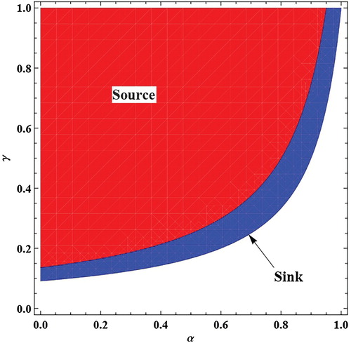
Next, for $\alpha \in [0,2]$ and $\gamma \in [0,2]$ the aforementioned topological classification for $P_0$ is depicted in Figure 2. Moreover, for the existence of boundary equilibrium $P_1$, we assume that $0<\alpha <1$, then the Jacobian matrix $J(x,y)$ at $P_1$ is computed as follows: $J(P_1):=\left(\begin{array}{cc}\alpha & 0\\ 0& {\displaystyle \frac{\gamma (1-\alpha +\beta )}{\beta }}\end{array}\right).$ Furthermore, topological classification for boundary equilibrium $P_1$ is itemized as follows:

• $P_1$ is a sink if and only if $0<\alpha <1$ and $0<\gamma <\beta /(1-\alpha +\beta )$.

• $P_1$ is a saddle point if and only if $0<\alpha <1$ and $\gamma >\beta /(1-\alpha +\beta )$.

• $P_1$ is a non-hyperbolic point if and only if $\gamma =\beta /(1-\alpha +\beta )$.

Figure 2. Topological classification of $P_0$ for $\alpha \in [0,2]$ and $\gamma \in [0,2]$.

Furthermore, for $\alpha \in [0,1]$, $\beta \in [0,200]$ and $\gamma =0.995$ the topological classification of $P_1$ is depicted in Figure 3. At the end of this section, we explore dynamics of model (1(1) $\begin{array}{rl}{x}_{n+1}& =\frac{x_n}{\alpha (1+y_n^2)+\beta x_n},\\ y_{n+1}& =\gamma y_n(1+x_n),\end{array}$(1) ) at its unique positive steady-state $P_{\ast }$. For this, first Jacobian matrix at this equilibrium is computed as follows: $J(P_{\ast }):=\left(\begin{array}{cc}1+\beta -{\displaystyle \frac{\beta }{\gamma }}& {\displaystyle \frac{2(\gamma -1)\sqrt{\alpha (\beta (\gamma -1)+\gamma -\alpha \gamma )}}{{\gamma }^{3/2}}}\\ \sqrt{\frac{\gamma (\beta (\gamma -1)+\gamma -\alpha \gamma )}{\alpha }}& 1\end{array}\right).$ Moreover, characteristic polynomial for $J(P_{\ast })$ is computed as follows: (4) $F(\lambda )={\lambda }^2-(2-\beta (\frac{1}{\gamma }-1))\lambda +3+5\beta -2\alpha (1-\gamma )-\frac{3\beta }{\gamma }-2\gamma (1+\beta ).$(4) From (4(4) $F(\lambda )={\lambda }^2-(2-\beta (\frac{1}{\gamma }-1))\lambda +3+5\beta -2\alpha (1-\gamma )-\frac{3\beta }{\gamma }-2\gamma (1+\beta ).$(4) ) we have $F(1)=\frac{2(1-\gamma )(\beta (\gamma -1)+\gamma -\alpha \gamma )}{\gamma }$ and $F(-1)=6+6\beta -2\alpha (1-\gamma )-\frac{4\beta }{\gamma }-2(1+\beta )\gamma .$ Assume that $0<\alpha <1,\beta >0$, and $\beta /(1-\alpha +\beta )<\gamma <1$, then from first part of last inequality we have $\beta <\gamma (1-\alpha +\beta )$, or equivalently $\beta (\gamma -1)+\gamma -\alpha \gamma >0$. Hence, it follows that $F(1)>0$. Similarly, one can prove that $F(-1)>0$ under the existence conditions for positive steady-state $P_{\ast }$ of system (1(1) $\begin{array}{rl}{x}_{n+1}& =\frac{x_n}{\alpha (1+y_n^2)+\beta x_n},\\ y_{n+1}& =\gamma y_n(1+x_n),\end{array}$(1) ). That is, $F(-1)>0$ for $0<\alpha <1,\beta >0$, and $\beta /(1-\alpha +\beta )<\gamma <1$. Indeed, it follows that $\begin{array}{rl}F(-1)& =6+6\beta -2\alpha (1-\gamma )-\frac{4\beta }{\gamma }-2(1+\beta )\gamma \\ & =2+6\beta -2\alpha (1-\gamma )-\frac{4\beta }{\gamma }-2(1+\beta )\gamma +4\\ & =2(1-\gamma )(1-\alpha +\beta )-4(1-\gamma )\left(\frac{\beta }{\gamma }\right)+4\\ & >2(1-\gamma )\left(\frac{\beta }{\gamma }\right)-4(1-\gamma )\left(\frac{\beta }{\gamma }\right)+4\\ & =2(2+\beta -\frac{\beta }{\gamma })>2(1+\alpha )>0.\end{array}$ Therefore, according to Jury condition roots of $F(\lambda )=0$ inside the unit open disk if and only if $F(0)<1$, which on simplification gives that $2\alpha +\beta >2$, or $\gamma <3\beta /(2-2\alpha +2\beta )$ and $2\alpha +\beta \le 2$. Similarly, $F(0)>1$ if and only if $2\alpha +\beta <2$ and $3\beta /(2-2\alpha +2\beta )<\gamma$. Moreover, $F(0)=1$ if and only if $\gamma =3\beta /(2-2\alpha +2\beta )$ and $2\alpha +\beta <2$. Due to aforementioned computations, we have the following results:

Lemma 2.1

Assume that $0<\alpha <1,\beta >0$, and $\beta /(1-\alpha +\beta )<\gamma <1$, then the following conditions hold true:

• $P_{\ast }$ is a sink if and only if $2\alpha +\beta >2$, or $\gamma <3\beta /(2-2\alpha +2\beta )$ and $2\alpha +\beta \le 2$.

• $P_{\ast }$ is a source if and only if $2\alpha +\beta <2$ and $3\beta /(2-2\alpha +2\beta )<\gamma$.

• $P_{\ast }$ is a non-hyperbolic fixed point if and only if $\gamma =3\beta /(2-2\alpha +2\beta )$ and $2\alpha +\beta <2$.

In Figure 4, topological classification of $P_{\ast }$ is depicted for $0<\alpha <1$, $0<\gamma <1$ and $\beta =0.1$.

Figure 3. Topological classification of $P_1$ for $\alpha \in [0,1]$, $\beta \in [0,200]$ and $\gamma =0.995$.

Figure 4. Topological classification of $P_{\ast }$ for $0<\alpha <1$, $0<\gamma <1$ and $\beta =0.1$.

3. Transcritical bifurcation

In this section, we investigate that boundary equilibrium $P_1$ undergoes transcritical bifurcation. For this, we assume that $\gamma \equiv {\gamma }_0:=\frac{\beta }{1-\alpha +\beta }.$ Consider the set ${\mathrm{\Omega }}_{TB}$ given by ${\mathrm{\Omega }}_{TB}:=\{(\alpha ,\beta ,{\gamma }_0)\in {\mathbb{R}}_{+}^3:{\gamma }_0=\frac{\beta }{1-\alpha +\beta },0<\alpha <1,\beta >0\}.$ Assume that $(\alpha ,\beta ,{\gamma }_0)\in {\mathrm{\Omega }}_{TB}$, then system (1(1) $\begin{array}{rl}{x}_{n+1}& =\frac{x_n}{\alpha (1+y_n^2)+\beta x_n},\\ y_{n+1}& =\gamma y_n(1+x_n),\end{array}$(1) ) is equivalently represented by the following 2-dimensional map: (5) $\left(\begin{array}{c}u\\ v\end{array}\right)\to \left(\begin{array}{c}{\displaystyle \frac{u}{\alpha (1+v^2)+\beta u}}\\ ({\gamma }_0+\overline{\gamma })v(1+u)\end{array}\right),$(5) where $\overline{\gamma }$ is very small perturbation in ${\gamma }_0$. Furthermore, if we consider $x=u-(1-\alpha )/\beta$ and y=v, then map (5(5) $\left(\begin{array}{c}u\\ v\end{array}\right)\to \left(\begin{array}{c}{\displaystyle \frac{u}{\alpha (1+v^2)+\beta u}}\\ ({\gamma }_0+\overline{\gamma })v(1+u)\end{array}\right),$(5) ) is transformed into the following map: (6) $\left(\begin{array}{c}x\\ y\end{array}\right)\to \left(\begin{array}{c}{\displaystyle \frac{x+\frac{1-\alpha }{\beta }}{\alpha (1+y^2)+\beta (x+\frac{1-\alpha }{\beta })}}({\gamma }_0+\overline{\gamma })y(1+x+\frac{1-\alpha }{\beta })\end{array}\right).$(6) An application of Taylor series expansion about $(x,y,\overline{\gamma })=(0,0,0)$ yields that (7) $\left(\begin{array}{c}x\\ y\end{array}\right)\to \left(\begin{array}{cc}\alpha & 0\\ 0& {\displaystyle \frac{{\gamma }_0(1-\alpha +\beta )}{\beta }}\end{array}\right)\left(\begin{array}{c}x\\ y\end{array}\right)+\left(\begin{array}{c}f(x,y)\\ g(x,y,\overline{\gamma })\end{array}\right),$(7) where $f(x,y)=-\alpha \beta x^2-\frac{\alpha (1-\alpha )}{\beta }{y}^2+\alpha {\beta }^2{x}^3+\alpha (1-2\alpha )x{y}^2+O((|x|+|y|{)}^4)$ and $g(x,y,\overline{\gamma })={\gamma }_{0}xy+\left(\frac{1-\alpha +\beta }{\beta }\right)y\overline{\gamma }+xy\overline{\gamma }.$ Since at ${\gamma }_0=\beta /(1-\alpha +\beta )$ the linear part of map (7(7) $\left(\begin{array}{c}x\\ y\end{array}\right)\to \left(\begin{array}{cc}\alpha & 0\\ 0& {\displaystyle \frac{{\gamma }_0(1-\alpha +\beta )}{\beta }}\end{array}\right)\left(\begin{array}{c}x\\ y\end{array}\right)+\left(\begin{array}{c}f(x,y)\\ g(x,y,\overline{\gamma })\end{array}\right),$(7) ) is already in canonical form. Therefore, in order to implement the centre manifold theorem [9], let $W^C(0,0,0)$ denotes the centre manifold for the map (7(7) $\left(\begin{array}{c}x\\ y\end{array}\right)\to \left(\begin{array}{cc}\alpha & 0\\ 0& {\displaystyle \frac{{\gamma }_0(1-\alpha +\beta )}{\beta }}\end{array}\right)\left(\begin{array}{c}x\\ y\end{array}\right)+\left(\begin{array}{c}f(x,y)\\ g(x,y,\overline{\gamma })\end{array}\right),$(7) ) which is evaluated at $(0,0)$ in a small neighbourhood of $\overline{\gamma }=0$. Then, $W^C(0,0,0)$ is computed as follows: $W^C(0,0,0)=\{(x,y,\overline{\gamma })\in {\mathbb{R}}^3:y=m_1{x}^2+m_{2}x\overline{\gamma }+m_3{\overline{\gamma }}^2+O((|x|+|\overline{\gamma }|{)}^3)\},$ where $m_1=m_2=m_3=0.$ Moreover, we define the following mapping which is restricted to the centre manifold $W^C(0,0,0)$: $F:x\to x+\overline{\gamma }+s_1{x}^2+s_{2}x\overline{\gamma }+s_3{\overline{\gamma }}^2+O((|x|+|\overline{\gamma }|{)}^3),$ where $s_1=-\alpha \beta ,s_2=s_3=0.$ Furthermore, it follows that $F(0,0)=0,F_x(0,0)=1,F_{\overline{\gamma }}(0,0)=1,F_{xx}(0,0)=-2\alpha \beta <0.$ Then, the following theorem gives the parametric conditions for existence and direction of transcritical bifurcation for system (1(1) $\begin{array}{rl}{x}_{n+1}& =\frac{x_n}{\alpha (1+y_n^2)+\beta x_n},\\ y_{n+1}& =\gamma y_n(1+x_n),\end{array}$(1) ) at its boundary fixed point $P_1$.

Theorem 3.1

Suppose that $\gamma =\beta /(1-\alpha +\beta )$ and $0<\alpha <1$, then system (1(1) $\begin{array}{rl}{x}_{n+1}& =\frac{x_n}{\alpha (1+y_n^2)+\beta x_n},\\ y_{n+1}& =\gamma y_n(1+x_n),\end{array}$(1) ) undergoes transcritical bifurcation at its boundary steady-state $P_1$ when parameter γ varies in a small neighbourhood of ${\gamma }_0=\beta /(1-\alpha +\beta )$. Furthermore, two steady-states bifurcate from $P_1$ for $\gamma <{\gamma }_0$, and merge as the steady-state $P_1$ at $\gamma ={\gamma }_0$ and disappear at $\gamma >{\gamma }_0$.

4. Neimark–Sacker bifurcation

In this section, we study that unique positive steady-state of system (1(1) $\begin{array}{rl}{x}_{n+1}& =\frac{x_n}{\alpha (1+y_n^2)+\beta x_n},\\ y_{n+1}& =\gamma y_n(1+x_n),\end{array}$(1) ) undergoes Neimark–Sacker bifurcation. For this, necessary conditions for existence of Neimark–Sacker bifurcation at $P_{\ast }$ are given as follows: $\gamma =\frac{3\beta }{2-2\alpha +2\beta },2\alpha +\beta <2.$ Next, we consider the following set: ${\mathbf{S}}_{NB}:=\{(\alpha ,\beta ,{\gamma }_1)\in {\mathbb{R}}_{+}^3:{\gamma }_1=\frac{3\beta }{2-2\alpha +2\beta },2\alpha +\beta <2,0<\alpha <1,\beta >0\}.$ Assume that $(\alpha ,\beta ,{\gamma }_1)\in {\mathbf{S}}_{NB}$, and $\tilde{\gamma }$ be small perturbation in ${\gamma }_1$, then system (1(1) $\begin{array}{rl}{x}_{n+1}& =\frac{x_n}{\alpha (1+y_n^2)+\beta x_n},\\ y_{n+1}& =\gamma y_n(1+x_n),\end{array}$(1) ) can be expressed by the following two-dimensional perturbed map: (8) $\left(\begin{array}{c}u\\ v\end{array}\right)\to \left(\begin{array}{c}{\displaystyle \frac{u}{\alpha (1+v^2)+\beta u}}\\ ({\gamma }_1+\tilde{\gamma })v(1+u)\end{array}\right).$(8) In order to translate the unique positive fixed point $(\frac{1-({\gamma }_1+\tilde{\gamma })}{{\gamma }_1+\tilde{\gamma }},\sqrt{\frac{({\gamma }_1+\tilde{\gamma })(1+\beta )-(\alpha ({\gamma }_1+\tilde{\gamma })+\beta )}{\alpha ({\gamma }_1+\tilde{\gamma })}})$ of the perturbed map (8(8) $\left(\begin{array}{c}u\\ v\end{array}\right)\to \left(\begin{array}{c}{\displaystyle \frac{u}{\alpha (1+v^2)+\beta u}}\\ ({\gamma }_1+\tilde{\gamma })v(1+u)\end{array}\right).$(8) ) at origin, we consider the following translations: (9) $x=u-\frac{1-({\gamma }_1+\tilde{\gamma })}{{\gamma }_1+\tilde{\gamma }},y=v-\sqrt{\frac{({\gamma }_1+\tilde{\gamma })(1+\beta )-(\alpha ({\gamma }_1+\tilde{\gamma })+\beta )}{\alpha ({\gamma }_1+\tilde{\gamma })}}.$(9) Then, from (8(8) $\left(\begin{array}{c}u\\ v\end{array}\right)\to \left(\begin{array}{c}{\displaystyle \frac{u}{\alpha (1+v^2)+\beta u}}\\ ({\gamma }_1+\tilde{\gamma })v(1+u)\end{array}\right).$(8) ) and (9(9) $x=u-\frac{1-({\gamma }_1+\tilde{\gamma })}{{\gamma }_1+\tilde{\gamma }},y=v-\sqrt{\frac{({\gamma }_1+\tilde{\gamma })(1+\beta )-(\alpha ({\gamma }_1+\tilde{\gamma })+\beta )}{\alpha ({\gamma }_1+\tilde{\gamma })}}.$(9) ) it follows that (10) $\left(\begin{array}{c}x\\ y\end{array}\right)\to \left(\begin{array}{cc}{a}_{11}& a_{12}\\ a_{21}& a_{22}\end{array}\right)\left(\begin{array}{c}x\\ y\end{array}\right)+\left(\begin{array}{c}{f}_2(x,y)\\ g_2(x,y)\end{array}\right),$(10) where $\begin{array}{rl}\left(\begin{array}{cc}{a}_{11}& a_{12}\\ a_{21}& a_{22}\end{array}\right)& =(\begin{array}{c}1+\beta -\frac{\beta }{{\gamma }_1+\tilde{\gamma }}\\ \sqrt{\frac{({\gamma }_1+\tilde{\gamma })(\beta (({\gamma }_1+\tilde{\gamma })-1)+({\gamma }_1+\tilde{\gamma })-\alpha ({\gamma }_1+\tilde{\gamma }))}{\alpha }}\end{array}\\ & \times \begin{array}{c}\frac{2(({\gamma }_1+\tilde{\gamma })-1)\sqrt{\alpha (\beta (({\gamma }_1+\tilde{\gamma })-1)+({\gamma }_1+\tilde{\gamma })-\alpha ({\gamma }_1+\tilde{\gamma }))}}{({\gamma }_1+\tilde{\gamma }{)}^{3/2}}\\ 1\end{array}),\\ f_2(x,y)& =-\left(\frac{\alpha \beta +\alpha \beta Y^2}{{(\alpha +\beta X+\alpha Y^2)}^3}\right)x^2-\left(\frac{2\alpha Y(\alpha -\beta X+\alpha Y^2)}{{(\alpha +\beta X+\alpha Y^2)}^3}\right)xy\\ & -\left(\frac{X({\alpha }^2+\alpha \beta X-3{\alpha }^2{Y}^2)}{{(\alpha +\beta X+\alpha Y^2)}^3}\right)y^2+\left(\frac{\alpha {\beta }^2+\alpha {\beta }^2{Y}^2}{{(\alpha +\beta X+\alpha Y^2)}^4}\right)x^3\\ & +\left(\frac{2\alpha Y(2\alpha \beta -{\beta }^{2}X+2\alpha \beta Y^2)}{{(\alpha +\beta X+\alpha Y^2)}^4}\right)x^{2}y\\ & +\left(\frac{\alpha {\beta }^2{X}^2-{\alpha }^3-8{\alpha }^2\beta X{Y}^2+3{\alpha }^3{Y}^4+2{\alpha }^3{Y}^2}{{(\alpha +\beta X+\alpha Y^2)}^4}\right)x{y}^2\\ & +\left(\frac{4X({\alpha }^2\beta XY-{\alpha }^3{Y}^3+{\alpha }^{3}Y)}{{(\alpha +\beta X+\alpha Y^2)}^4}\right)y^3+O((|x|+|y|{)}^4),\\ g_2(x,y)& =({\gamma }_1+\tilde{\gamma })xy,X=\frac{1-({\gamma }_1+\tilde{\gamma })}{{\gamma }_1+\tilde{\gamma }},\\ Y& =\sqrt{\frac{({\gamma }_1+\tilde{\gamma })(1+\beta )-(\alpha ({\gamma }_1+\tilde{\gamma })+\beta )}{\alpha ({\gamma }_1+\tilde{\gamma })}}.\end{array}$ Moreover, the characteristic polynomial for $\left(\begin{array}{cc}{a}_{11}& a_{12}\\ a_{21}& a_{22}\end{array}\right)$ is computed as follows: (11) $\begin{array}{rl}P(\rho )& ={\rho }^2-(2-\beta (\frac{1}{{\gamma }_1+\tilde{\gamma }}-1))\rho +3+5\beta -2\alpha (1-({\gamma }_1+\tilde{\gamma }))\\ & -\frac{3\beta }{{\gamma }_1+\tilde{\gamma }}-2({\gamma }_1+\tilde{\gamma })(1+\beta ).\end{array}$(11) Assume that $\rho (\tilde{\gamma })$ and $\overline{\rho }(\tilde{\gamma })$ be complex conjugate roots of (11(11) $\begin{array}{rl}P(\rho )& ={\rho }^2-(2-\beta (\frac{1}{{\gamma }_1+\tilde{\gamma }}-1))\rho +3+5\beta -2\alpha (1-({\gamma }_1+\tilde{\gamma }))\\ & -\frac{3\beta }{{\gamma }_1+\tilde{\gamma }}-2({\gamma }_1+\tilde{\gamma })(1+\beta ).\end{array}$(11) ), then a simple computation yields that $|\rho (\tilde{\gamma })|=\sqrt{3-2\alpha +2\beta +2(\alpha -1-\beta )\tilde{\gamma }-\frac{6\beta (1-\alpha +\beta )}{3\beta +2(1-\alpha +\beta )\tilde{\gamma }}}.$ Furthermore, it follows that $|\rho (0)|=1$, but ${\rho }^i(0)\ne 1$ for all i=1,2,3,4 if and only if (12) $-\frac{1}{3}(4+2\alpha +\beta )\ne -2,0,1,2.$(12) Since $-\frac{1}{3}(4+2\alpha +\beta )<0$ and $(\alpha ,\beta ,{\gamma }_1)\in {\mathbf{S}}_{NB}$, therefore $-\frac{1}{3}(4+2\alpha +\beta )\ne -2$. Hence, condition (12(12) $-\frac{1}{3}(4+2\alpha +\beta )\ne -2,0,1,2.$(12) ) is satisfied. Moreover, it follows that ${\left(\frac{\mathrm{d}|\rho (\tilde{\gamma })|}{\mathrm{d}\tilde{\gamma }}\right)}_{\tilde{\gamma }=0}=\frac{(1-\alpha +\beta )(2-2\alpha -\beta )}{3\beta }>0.$ The following similarity transformation is considered in order to convert linear part of (10(10) $\left(\begin{array}{c}x\\ y\end{array}\right)\to \left(\begin{array}{cc}{a}_{11}& a_{12}\\ a_{21}& a_{22}\end{array}\right)\left(\begin{array}{c}x\\ y\end{array}\right)+\left(\begin{array}{c}{f}_2(x,y)\\ g_2(x,y)\end{array}\right),$(10) ) into canonical form at $\tilde{\gamma }=0$: (13) $\left(\begin{array}{c}x\\ y\end{array}\right)=\left(\begin{array}{cc}{a}_{12}& 0\\ \vartheta -a_{11}& -\phi \end{array}\right)\left(\begin{array}{c}w\\ z\end{array}\right),$(13) where $\vartheta :=\frac{4+2\alpha +\beta }{6},\phi :=\frac{\sqrt{(2-2\alpha -\beta )(10+2\alpha +\beta )}}{6}$ and $a_{11}=\frac{1}{3}(1+2\alpha +\beta ),a_{12}=\frac{2\alpha \sqrt{\frac{1-\alpha +\beta }{\alpha }}(2\alpha -2+\beta )}{3\sqrt{3}\beta }.$ Then, from transformation (13(13) $\left(\begin{array}{c}x\\ y\end{array}\right)=\left(\begin{array}{cc}{a}_{12}& 0\\ \vartheta -a_{11}& -\phi \end{array}\right)\left(\begin{array}{c}w\\ z\end{array}\right),$(13) ) it follows that (14) $\left(\begin{array}{c}w\\ z\end{array}\right)=\left(\begin{array}{cc}{\displaystyle \frac{1}{a_{12}}}& 0\\ {\displaystyle \frac{\vartheta -a_{11}}{\phi a_{12}}}& -{\displaystyle \frac{1}{\phi }}\end{array}\right)\left(\begin{array}{c}x\\ y\end{array}\right).$(14) Assuming $\tilde{\gamma }=0$, then from (10(10) $\left(\begin{array}{c}x\\ y\end{array}\right)\to \left(\begin{array}{cc}{a}_{11}& a_{12}\\ a_{21}& a_{22}\end{array}\right)\left(\begin{array}{c}x\\ y\end{array}\right)+\left(\begin{array}{c}{f}_2(x,y)\\ g_2(x,y)\end{array}\right),$(10) ), (13(13) $\left(\begin{array}{c}x\\ y\end{array}\right)=\left(\begin{array}{cc}{a}_{12}& 0\\ \vartheta -a_{11}& -\phi \end{array}\right)\left(\begin{array}{c}w\\ z\end{array}\right),$(13) ) and (14(14) $\left(\begin{array}{c}w\\ z\end{array}\right)=\left(\begin{array}{cc}{\displaystyle \frac{1}{a_{12}}}& 0\\ {\displaystyle \frac{\vartheta -a_{11}}{\phi a_{12}}}& -{\displaystyle \frac{1}{\phi }}\end{array}\right)\left(\begin{array}{c}x\\ y\end{array}\right).$(14) ) we obtain the following normal form of map (10(10) $\left(\begin{array}{c}x\\ y\end{array}\right)\to \left(\begin{array}{cc}{a}_{11}& a_{12}\\ a_{21}& a_{22}\end{array}\right)\left(\begin{array}{c}x\\ y\end{array}\right)+\left(\begin{array}{c}{f}_2(x,y)\\ g_2(x,y)\end{array}\right),$(10) ): (15) $\left(\begin{array}{c}w\\ z\end{array}\right)=\left(\begin{array}{cc}\vartheta & -\phi \\ \phi & \vartheta \end{array}\right)\left(\begin{array}{c}w\\ z\end{array}\right)+\left(\begin{array}{c}F(w,z)\\ G(w,z)\end{array}\right),$(15) where $F(w,z):=-\left(\frac{3\sqrt{3}\beta \sqrt{\frac{\beta }{1-\alpha +\beta }}}{2\sqrt{\alpha \beta }(2-2\alpha -\beta )}\right)f_2(a_{12}w,(\vartheta -a_{11})w-\phi z)$ and $G(w,z):=-\frac{\begin{array}{c}3(4\sqrt{\alpha \beta }{g}_2(a_{12}w,(\vartheta -a_{11})w-\phi z)\\ +\sqrt{3}\beta \sqrt{\frac{\beta }{1-\alpha +\beta }}{f}_2(a_{12}w,(\vartheta -a_{11})w-\phi z))\end{array}}{2\sqrt{\alpha \beta }\sqrt{(2-2\alpha -\beta )(10+2\alpha +\beta )}}.$ Taking into account the bifurcation theory of normal forms [28,36,43,48,49], the first Lyapunov exponent at $(w,z)=(0,0)$ is computed as follows: $L=-Re\left(\frac{(1-2\rho (0))\overline{\rho }(0{)}^2}{1-\rho (0)}{\tau }_{20}{\tau }_{11}\right)-\frac{1}{2}|{\tau }_{11}{|}^2-|{\tau }_{02}{|}^2+Re(\overline{\rho }(0){\tau }_{21}),$ where $\begin{array}{rl}{\tau }_{20}& =\frac{1}{8}[F_{ww}-F_{zz}+2G_{wz}+i(G_{ww}-G_{zz}-2F_{wz})],\\ {\tau }_{11}& =\frac{1}{4}[F_{ww}+F_{zz}+i(G_{ww}+G_{zz})],\\ {\tau }_{02}& =\frac{1}{8}[F_{ww}-F_{zz}-2G_{wz}+i(G_{ww}-G_{zz}+2F_{wz})],\end{array}$ and ${\tau }_{21}=\frac{1}{16}[F_{www}+F_{wzz}+G_{wwz}+G_{zzz}+i(G_{www}+G_{wzz}-F_{wwz}-F_{zzz})].$ Due to aforementioned computations, we have the following theorem:

Theorem 4.1

Suppose that $L\ne 0$, $0<\alpha <1$, $\beta /(1-\alpha +\beta )<\gamma <1$ and $2\alpha +\beta <2$, then unique positive equilibrium point $P_{\ast }$ of system (1(1) $\begin{array}{rl}{x}_{n+1}& =\frac{x_n}{\alpha (1+y_n^2)+\beta x_n},\\ y_{n+1}& =\gamma y_n(1+x_n),\end{array}$(1) ) undergoes Neimark–Sacker bifurcation when the bifurcation parameter γ varies in a small neighbourhood of ${\gamma }_1=3\beta /(2-2\alpha +2\beta )$. Moreover, if L<0, then an attracting invariant closed curve bifurcates from the equilibrium point for $\gamma >{\gamma }_1$, and if L>0, then a repelling invariant closed curve bifurcates from the equilibrium point for $\gamma <{\gamma }_1$.

5. Chaos control

Chaos control is a method of stabilization with the help of small perturbations which are applied to unstable periodic orbits for a given system. The purpose of chaos control is to make chaotic behaviour more predictable and stable. For this, a small perturbation is applied as compare to the original size of the system under consideration, and in a result the natural dynamics of the system is prevented from any major modification. Recently, chaos control for irregular complex dynamics has developed as one of the leading topics in nonlinear applied science. The pioneer articles related to chaos control were published in 1990 and after that their number has been steadily increasing [46]. Moreover, the practical methods related to chaos control can be implemented in various areas such as communications, physics laboratories, biochemistry, turbulence, and cardiology [40]. Furthermore, in the case of dynamical systems related to biological breeding of species, chaos control is considered to be an important feature for investigation. On the other hand, population models with non-overlapping generations have more irregular complex behaviour. For some recent investigation related to chaos control in discrete-time models we refer to [1,13–20,22–24] and references are therein.

In this section, first we discuss pole-placement chaos control method based on state feedback control which was introduced by Romeiras et al. [44] (also see [41]). This method is also known as generalized or modified OGY method proposed by Ott et al. [42]. For the application of pole-placement technique to model (1(1) $\begin{array}{rl}{x}_{n+1}& =\frac{x_n}{\alpha (1+y_n^2)+\beta x_n},\\ y_{n+1}& =\gamma y_n(1+x_n),\end{array}$(1) ), one can rewrite this system as follows: (16) $\begin{array}{rl}{x}_{n+1}& =\frac{x_n}{\alpha (1+y_n^2)+\beta x_n}=f(x_n,y_n,\gamma ),\\ y_{n+1}& =\gamma y_n(1+x_n)=g(x_n,y_n,\gamma ),\end{array}$(16) where γ denotes parameter for chaos control. Furthermore, it is assumed that γ lies in a small interval of type $|\gamma -{\gamma }_0|<\delta$, where $\delta >0$ and ${\gamma }_0$ represents the nominal parameter lies in the chaotic region. One can apply pole-placement method in order to move unstable trajectory towards desired stable orbit. For this, suppose that $(x^{\ast },y^{\ast })$ be an unstable fixed point for model (1(1) $\begin{array}{rl}{x}_{n+1}& =\frac{x_n}{\alpha (1+y_n^2)+\beta x_n},\\ y_{n+1}& =\gamma y_n(1+x_n),\end{array}$(1) ) lies in a chaotic region under the influence of transcritical or Neimark–Sacker bifurcations. Keeping in view the method of linearization, one can approximate system (16(16) $\begin{array}{rl}{x}_{n+1}& =\frac{x_n}{\alpha (1+y_n^2)+\beta x_n}=f(x_n,y_n,\gamma ),\\ y_{n+1}& =\gamma y_n(1+x_n)=g(x_n,y_n,\gamma ),\end{array}$(16) ) in the neighbourhood of the unstable fixed point $(x^{\ast },y^{\ast })$ as follows: (17) $\left[\begin{array}{c}{x}_{n+1}-x^{\ast }\\ y_{n+1}-y^{\ast }\end{array}\right]\approx A\left[\begin{array}{c}{x}_n-x^{\ast }\\ y_n-y^{\ast }\end{array}\right]+B[\gamma -{\gamma }_0],$(17) where $A=\left[\begin{array}{cc}{\displaystyle \frac{\mathrm{\partial }f(x^{\ast },y^{\ast },{\gamma }_0)}{\mathrm{\partial }{x}_n}}& {\displaystyle \frac{\mathrm{\partial }f(x^{\ast },y^{\ast },{\gamma }_0)}{\mathrm{\partial }{y}_n}}\\ {\displaystyle \frac{\mathrm{\partial }g(x^{\ast },y^{\ast },{\gamma }_0)}{\mathrm{\partial }{y}_n}}& {\displaystyle \frac{\mathrm{\partial }g(x^{\ast },y^{\ast },{\gamma }_0)}{\mathrm{\partial }{y}_n}}\end{array}\right],B=\left[\begin{array}{c}{\displaystyle \frac{\mathrm{\partial }f(x^{\ast },y^{\ast },{\gamma }_0)}{\mathrm{\partial }\gamma }}\\ {\displaystyle \frac{\mathrm{\partial }g(x^{\ast },y^{\ast },{\gamma }_0)}{\mathrm{\partial }\gamma }}\end{array}\right]=\left[\begin{array}{c}0\\ y^{\ast }(1+x^{\ast })\end{array}\right].$ In order to check that system (16(16) $\begin{array}{rl}{x}_{n+1}& =\frac{x_n}{\alpha (1+y_n^2)+\beta x_n}=f(x_n,y_n,\gamma ),\\ y_{n+1}& =\gamma y_n(1+x_n)=g(x_n,y_n,\gamma ),\end{array}$(16) ) is controllable, the following matrix is computed: (18) $C=[B:AB]=\left[\begin{array}{ccc}0& \left({\displaystyle \frac{\mathrm{\partial }f(x^{\ast },y^{\ast },{\gamma }_0)}{\mathrm{\partial }{y}_n}}\right)(y^{\ast }(1+x^{\ast }))y^{\ast }(1+x^{\ast })& \left({\displaystyle \frac{\mathrm{\partial }g(x^{\ast },y^{\ast },{\gamma }_0)}{\mathrm{\partial }{y}_n}}\right)(y^{\ast }(1+x^{\ast }))\end{array}\right].$(18) Assume that $(x^{\ast },y^{\ast })$ is positive fixed point, then it follows that $y^{\ast }(1+x^{\ast })\ne 0$. Therefore, rank of C is 2 at positive equilibrium point. Next, we assume that $[\gamma -{\gamma }_0]=-K\left[\begin{array}{c}{x}_n-x^{\ast }\\ y_n-y^{\ast }\end{array}\right]$, where $K=\left[\begin{array}{cc}{k}_1& k_2\end{array}\right]$, then system (17(17) $\left[\begin{array}{c}{x}_{n+1}-x^{\ast }\\ y_{n+1}-y^{\ast }\end{array}\right]\approx A\left[\begin{array}{c}{x}_n-x^{\ast }\\ y_n-y^{\ast }\end{array}\right]+B[\gamma -{\gamma }_0],$(17) ) can be written as (19) $\left[\begin{array}{c}{x}_{n+1}-x^{\ast }\\ y_{n+1}-y^{\ast }\end{array}\right]\approx [A-BK]\left[\begin{array}{c}{x}_n-x^{\ast }\\ y_n-y^{\ast }\end{array}\right].$(19) Moreover, equilibrium point $(x^{\ast },y^{\ast })$ is a sink if and only if both eigenvalues ${\mu }_1$ and ${\mu }_2$ for the matrix A−BK lie in an open unit disk. Moreover, ${\mu }_1$ and ${\mu }_2$ are called regulator poles. Placing these eigenvalues at appropriate position is called pole-placement method. Furthermore, pole-placement problem has unique solution because rank of matrix C is two. Denote ${\lambda }^2+{\alpha }_1\lambda +{\alpha }_2=0$ as characteristic equation for matrix A and ${\mu }^2+{\beta }_1\mu +{\beta }_2=0$ is characteristic equation of A−BK, then unique solution of the pole-placement problem is given as follows: (20) $K=\left[\begin{array}{cc}{\beta }_2-{\alpha }_2& {\beta }_1-{\alpha }_1\end{array}\right]T^{-1},$(20) where T=CM and $M=\left[\begin{array}{cc}{\alpha }_1& 1\\ 1& 0\end{array}\right]$. Then it follows that (21) $T=CM=\left[\begin{array}{ccc}{\displaystyle \frac{\mathrm{\partial }f}{\mathrm{\partial }{y}_n}}{\displaystyle \frac{\mathrm{\partial }g}{\mathrm{\partial }\gamma }}& 0{\alpha }_1{\displaystyle \frac{\mathrm{\partial }g}{\mathrm{\partial }\gamma }}+{\displaystyle \frac{\mathrm{\partial }g}{\mathrm{\partial }{y}_n}}{\displaystyle \frac{\mathrm{\partial }g}{\mathrm{\partial }\gamma }}& {\displaystyle \frac{\mathrm{\partial }g}{\mathrm{\partial }\gamma }}\end{array}\right],$(21) where all partial derivatives in (21(21) $T=CM=\left[\begin{array}{ccc}{\displaystyle \frac{\mathrm{\partial }f}{\mathrm{\partial }{y}_n}}{\displaystyle \frac{\mathrm{\partial }g}{\mathrm{\partial }\gamma }}& 0{\alpha }_1{\displaystyle \frac{\mathrm{\partial }g}{\mathrm{\partial }\gamma }}+{\displaystyle \frac{\mathrm{\partial }g}{\mathrm{\partial }{y}_n}}{\displaystyle \frac{\mathrm{\partial }g}{\mathrm{\partial }\gamma }}& {\displaystyle \frac{\mathrm{\partial }g}{\mathrm{\partial }\gamma }}\end{array}\right],$(21) ) are evaluated at $(x^{\ast },y^{\ast },{\gamma }_0)$. From (20(20) $K=\left[\begin{array}{cc}{\beta }_2-{\alpha }_2& {\beta }_1-{\alpha }_1\end{array}\right]T^{-1},$(20) ) and (21(21) $T=CM=\left[\begin{array}{ccc}{\displaystyle \frac{\mathrm{\partial }f}{\mathrm{\partial }{y}_n}}{\displaystyle \frac{\mathrm{\partial }g}{\mathrm{\partial }\gamma }}& 0{\alpha }_1{\displaystyle \frac{\mathrm{\partial }g}{\mathrm{\partial }\gamma }}+{\displaystyle \frac{\mathrm{\partial }g}{\mathrm{\partial }{y}_n}}{\displaystyle \frac{\mathrm{\partial }g}{\mathrm{\partial }\gamma }}& {\displaystyle \frac{\mathrm{\partial }g}{\mathrm{\partial }\gamma }}\end{array}\right],$(21) ), we have the following unique solution of pole-placement problem: $k_1=\frac{{\beta }_2-{\alpha }_2}{\left(\frac{\mathrm{\partial }f(x^{\ast },y^{\ast },{\gamma }_0)}{\mathrm{\partial }{y}_n}\right)\left(\frac{\mathrm{\partial }g(x^{\ast },y^{\ast },{\gamma }_0)}{\mathrm{\partial }c}\right)}-\frac{({\beta }_1-{\alpha }_1)({\alpha }_1+\frac{\mathrm{\partial }g(x^{\ast },y^{\ast },{\gamma }_0)}{\mathrm{\partial }{y}_n})}{\left(\frac{\mathrm{\partial }f(x^{\ast },y^{\ast },{\gamma }_0)}{\mathrm{\partial }{y}_n}\right)\left(\frac{\mathrm{\partial }g(x^{\ast },y^{\ast },{\gamma }_0)}{\mathrm{\partial }\gamma }\right)},k_2=\frac{{\beta }_1-{\alpha }_1}{\frac{\mathrm{\partial }g(x^{\ast },y^{\ast },{\gamma }_0)}{\mathrm{\partial }\gamma }}.$ Secondly, we apply another comparatively simple chaos control method known as hybrid control strategy based on parameter perturbation and state feedback control [39,50]. An application of hybrid control strategy to model (1(1) $\begin{array}{rl}{x}_{n+1}& =\frac{x_n}{\alpha (1+y_n^2)+\beta x_n},\\ y_{n+1}& =\gamma y_n(1+x_n),\end{array}$(1) ) yields the following controlled system: (22) $\begin{array}{rl}{x}_{n+1}& =\kappa \left(\frac{x_n}{\alpha (1+y_n^2)+\beta x_n}\right)+(1-\kappa )x_n,\\ y_{n+1}& =\kappa (\gamma y_n(1+x_n))+(1-\kappa )y_n,\end{array}$(22) where $0<\kappa <1$ is control parameter. Assume that $(x^{\ast },y^{\ast })$ be an equilibrium point of system (22(22) $\begin{array}{rl}{x}_{n+1}& =\kappa \left(\frac{x_n}{\alpha (1+y_n^2)+\beta x_n}\right)+(1-\kappa )x_n,\\ y_{n+1}& =\kappa (\gamma y_n(1+x_n))+(1-\kappa )y_n,\end{array}$(22) ), then Jacobian matrix for system (22(22) $\begin{array}{rl}{x}_{n+1}& =\kappa \left(\frac{x_n}{\alpha (1+y_n^2)+\beta x_n}\right)+(1-\kappa )x_n,\\ y_{n+1}& =\kappa (\gamma y_n(1+x_n))+(1-\kappa )y_n,\end{array}$(22) ) computed at $(x^{\ast },y^{\ast })$ is given as follows: (23) $J(x^{\ast },y^{\ast }):=\left(\begin{array}{cc}{\displaystyle \frac{\kappa \alpha (1+(y^{\ast }{)}^2)}{{(\alpha (1+(y^{\ast }{)}^2)+\beta x^{\ast })}^2}}+1-\kappa & -{\displaystyle \frac{2\kappa \alpha x^{\ast }{y}^{\ast }}{{(\alpha (1+(y^{\ast }{)}^2)+\beta x^{\ast })}^2}}\\ \gamma \kappa y^{\ast }& \gamma \kappa (1+x^{\ast })+1-\kappa \end{array}\right).$(23) It is easy to observe that system (22(22) $\begin{array}{rl}{x}_{n+1}& =\kappa \left(\frac{x_n}{\alpha (1+y_n^2)+\beta x_n}\right)+(1-\kappa )x_n,\\ y_{n+1}& =\kappa (\gamma y_n(1+x_n))+(1-\kappa )y_n,\end{array}$(22) ) is controllable as long as the steady-state $(x^{\ast },y^{\ast })$ of system (22(22) $\begin{array}{rl}{x}_{n+1}& =\kappa \left(\frac{x_n}{\alpha (1+y_n^2)+\beta x_n}\right)+(1-\kappa )x_n,\\ y_{n+1}& =\kappa (\gamma y_n(1+x_n))+(1-\kappa )y_n,\end{array}$(22) ) is locally asymptotically stable. Keeping in view this fact, one has the following result for controllability of system (22(22) $\begin{array}{rl}{x}_{n+1}& =\kappa \left(\frac{x_n}{\alpha (1+y_n^2)+\beta x_n}\right)+(1-\kappa )x_n,\\ y_{n+1}& =\kappa (\gamma y_n(1+x_n))+(1-\kappa )y_n,\end{array}$(22) ).

Lemma 5.1

The equilibrium point $(x^{\ast },y^{\ast })$ of system (22(22) $\begin{array}{rl}{x}_{n+1}& =\kappa \left(\frac{x_n}{\alpha (1+y_n^2)+\beta x_n}\right)+(1-\kappa )x_n,\\ y_{n+1}& =\kappa (\gamma y_n(1+x_n))+(1-\kappa )y_n,\end{array}$(22) ) is locally asymptotically stable if the following holds true: $|TrJ(x^{\ast },y^{\ast })|<1+detJ(x^{\ast },y^{\ast })<2.$

6. Numerical simulation and discussion

First, we choose $\alpha =0.99$, $\beta =0.008$, $\gamma \in [0.2,0.7]$ and $(x_0,y_0)=(1.25,0.001)$. Then, system (1(1) $\begin{array}{rl}{x}_{n+1}& =\frac{x_n}{\alpha (1+y_n^2)+\beta x_n},\\ y_{n+1}& =\gamma y_n(1+x_n),\end{array}$(1) ) undergoes transcritical bifurcation at its boundary equilibrium point $(1.25,0)$ as bifurcation parameter γ passes through $\gamma \approx 0.4444$. Furthermore, at $\gamma \approx 0.666667$ the positive steady-state $(0.499999,0.0778499)$ exists and undergoes Neimark–Sacker bifurcation. At $(\alpha ,\beta ,\gamma )=(0.99,0.008,0.666667)$ the characteristic equation for Jacobian matrix of model (1(1) $\begin{array}{rl}{x}_{n+1}& =\frac{x_n}{\alpha (1+y_n^2)+\beta x_n},\\ y_{n+1}& =\gamma y_n(1+x_n),\end{array}$(1) ) is computed as follows: ${\lambda }^2-1.996\lambda +1=0.$ Obviously, ${\lambda }_1=0.998-0.0632139i$ and ${\lambda }_2=0.998+0.0632139i$ be roots for aforementioned characteristic equation with $|{\lambda }_{1,2}|=1$. The maximum Lyapunov exponents (MLE) and bifurcation diagrams are depicted in Figure 5. Secondly, we select $\alpha =0.2$, $\beta =0.5$, $\gamma \in [0.45,0.95]$ and $(x_0,y_0)=(0.78,1.426)$, then model (1(1) $\begin{array}{rl}{x}_{n+1}& =\frac{x_n}{\alpha (1+y_n^2)+\beta x_n},\\ y_{n+1}& =\gamma y_n(1+x_n),\end{array}$(1) ) undergoes Neimark–Sacker bifurcation at its positive steady-state $(0.733333,1.47196)$ as bifurcation parameter γ varies in a small neighbourhood of $\gamma =0.576923$. For the parametric values $(\alpha ,\beta ,\gamma )=(0.2,0.5,0.576923)$ the characteristic equation of the Jacobian matrix of system (1(1) $\begin{array}{rl}{x}_{n+1}& =\frac{x_n}{\alpha (1+y_n^2)+\beta x_n},\\ y_{n+1}& =\gamma y_n(1+x_n),\end{array}$(1) ) is computed as follows: ${\lambda }^2-1.63333\lambda +1=0.$ Moreover, we have ${\lambda }_1=0.816667-0.57711i$ and ${\lambda }_2=0.816667+0.57711i$ as roots for aforementioned characteristic equation with $|{\lambda }_{1,2}|=1$. 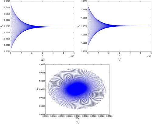MLE and bifurcation diagrams are depicted in Figure 6. On the other hand, some phase portraits for $\gamma =0.573,0.576923,0.58,0.65$ are depicted in Figure 7.

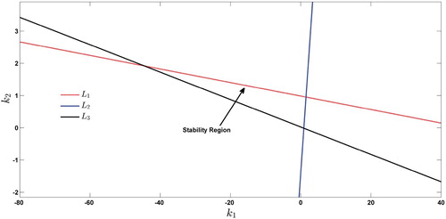
Finally, we take $\alpha =0.2$, $\beta =0.5$ and $\gamma =0.95$ to verify the effectiveness of chaos control strategies introduced in Section 5. Under this selection of parameters, system (1(1) $\begin{array}{rl}{x}_{n+1}& =\frac{x_n}{\alpha (1+y_n^2)+\beta x_n},\\ y_{n+1}& =\gamma y_n(1+x_n),\end{array}$(1) ) has unique positive steady-state given by $(0.0526316,1.96683)$. An application of pole-placement method gives the following controlled system: (24) $\begin{array}{rl}{x}_{n+1}& =\frac{x_n}{0.2(1+y_n^2)+0.5x_n},\\ y_{n+1}& =(0.95-k_1(x_n-0.0526316)-k_2(y_n-1.96683))y_n(1+x_n).\end{array}$(24) Then, variational matrix for system (24(24) $\begin{array}{rl}{x}_{n+1}& =\frac{x_n}{0.2(1+y_n^2)+0.5x_n},\\ y_{n+1}& =(0.95-k_1(x_n-0.0526316)-k_2(y_n-1.96683))y_n(1+x_n).\end{array}$(24) ) is computed as follows: $\left[\begin{array}{cc}0.973684& -0.041407\\ 1.86849-2.07035k_1& 1-2.07035k_2\end{array}\right].$ Furthermore, the lines for marginal stability are computed as follows: $\begin{array}{rl}& L_1:k_2=0.984955-0.0209795k_1,\\ & L_2:k_2=-1.42005+1.57346k_1,\end{array}$ and $L_3:k_2=0.0253254-0.0425261k_1.$ The triangular stability region bounded by these marginal stability lines is depicted in Figure 8.

Figure 5. Bifurcation diagrams and MLE for system (1(1) $\begin{array}{rl}{x}_{n+1}& =\frac{x_n}{\alpha (1+y_n^2)+\beta x_n},\\ y_{n+1}& =\gamma y_n(1+x_n),\end{array}$(1) ) with $\alpha =0.99$, $\beta =0.008$, $\gamma \in [0.2,0.7]$ and $(x_0,y_0)=(1.25,0.001)$: (a) bifurcation diagram for $x_n$, (b) bifurcation diagram for $y_n$ and (c) MLE.

Figure 6. Bifurcation diagrams and MLE for system (1(1) $\begin{array}{rl}{x}_{n+1}& =\frac{x_n}{\alpha (1+y_n^2)+\beta x_n},\\ y_{n+1}& =\gamma y_n(1+x_n),\end{array}$(1) ) with $\alpha =0.2$, $\beta =0.5$, $\gamma \in [0.45,0.95]$ and $(x_0,y_0)=(0.78,1.426)$: (a) bifurcation diagram for $x_n$, (b) bifurcation diagram for $y_n$ and (c) MLE.

Figure 7. Phase portraits of system (1(1) $\begin{array}{rl}{x}_{n+1}& =\frac{x_n}{\alpha (1+y_n^2)+\beta x_n},\\ y_{n+1}& =\gamma y_n(1+x_n),\end{array}$(1) ) for $\alpha =0.2$, $\beta =0.5$, $x_0=0.78,y_0=1.426$ and with different values of γ: (a) phase portrait for $\gamma =0.573$, (b) phase portrait for $\gamma =0.576923$, (c) phase portrait for $\gamma =0.58$ and (d) phase portrait for $\gamma =0.65$.

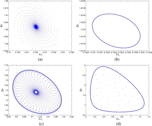
Figure 8. Bounded stability region for system (24(24) $\begin{array}{rl}{x}_{n+1}& =\frac{x_n}{0.2(1+y_n^2)+0.5x_n},\\ y_{n+1}& =(0.95-k_1(x_n-0.0526316)-k_2(y_n-1.96683))y_n(1+x_n).\end{array}$(24) ).

Next, for same parametric values we apply hybrid control method to system (1(1) $\begin{array}{rl}{x}_{n+1}& =\frac{x_n}{\alpha (1+y_n^2)+\beta x_n},\\ y_{n+1}& =\gamma y_n(1+x_n),\end{array}$(1) ). In this case system (22(22) $\begin{array}{rl}{x}_{n+1}& =\kappa \left(\frac{x_n}{\alpha (1+y_n^2)+\beta x_n}\right)+(1-\kappa )x_n,\\ y_{n+1}& =\kappa (\gamma y_n(1+x_n))+(1-\kappa )y_n,\end{array}$(22) ) is written as follows: (25) $\begin{array}{rl}{x}_{n+1}& =\kappa \left(\frac{x_n}{0.2(1+y_n^2)+0.5x_n}\right)+(1-\kappa )x_n,\\ y_{n+1}& =\kappa (0.95y_n(1+x_n))+(1-\kappa )y_n.\end{array}$(25) Then, Jacobian matrix of system (25(25) $\begin{array}{rl}{x}_{n+1}& =\kappa \left(\frac{x_n}{0.2(1+y_n^2)+0.5x_n}\right)+(1-\kappa )x_n,\\ y_{n+1}& =\kappa (0.95y_n(1+x_n))+(1-\kappa )y_n.\end{array}$(25) ) and its characteristic equation are computed as follows: $\left[\begin{array}{cc}1-0.0263158\kappa & -0.041407\kappa \\ 1.86849\kappa & 1\end{array}\right]$ and ${\lambda }^2-(2-0.0263158\kappa )\lambda +1-0.0263158\kappa +0.0773684{\kappa }^2=0.$ Keeping in view Jury condition and aforementioned characteristic equation, $|2-0.0263158\kappa |<2-0.0263158\kappa +0.0773684{\kappa }^2<2$ if and only if $0<\kappa <0.340136$. At $\kappa =0.33$ the plots for system (25(25) $\begin{array}{rl}{x}_{n+1}& =\kappa \left(\frac{x_n}{0.2(1+y_n^2)+0.5x_n}\right)+(1-\kappa )x_n,\\ y_{n+1}& =\kappa (0.95y_n(1+x_n))+(1-\kappa )y_n.\end{array}$(25) ) are depicted in Figure 9.

Figure 9. Plots for system (25(25) $\begin{array}{rl}{x}_{n+1}& =\kappa \left(\frac{x_n}{0.2(1+y_n^2)+0.5x_n}\right)+(1-\kappa )x_n,\\ y_{n+1}& =\kappa (0.95y_n(1+x_n))+(1-\kappa )y_n.\end{array}$(25) ) with $\kappa =0.33$ and $(x_0,y_0)=(0.0526316,1.96683)$: (a) plot for $x_n$, (b) plot for $y_n$ and (c) phase portrait.

7. Concluding remarks

Local asymptotic stability, bifurcation analysis and chaos control are investigated for the apple twig borer and the grape vine type plant–herbivore model. The discrete-time model is obtained by taking into account the weak predator functional response. Furthermore, existence of equilibria and their stability analysis is investigated. Taking into account the bifurcating behaviour for biological populations, it must be noted that these phenomena are essential for competition between plants and herbivores [11]. It is proved that plant–herbivore model undergoes transcritical bifurcation at its boundary equilibrium by implementing bifurcation theory of normal forms and centre manifold theorem. Direction and existence criteria for Neimark–Sacker bifurcation are investigated at positive steady-state of plant–herbivore model. Bifurcating behaviour and chaos have always been considered as disadvantageous phenomena in biology. On the other hand, due to chaotic behaviour population can undergo a higher risk of extinction due to the unpredictability. Therefore, these are catastrophic for the breeding of biological population [51]. In order to prevent biological populations from this ruinous situation, one might think about applications of chaos and bifurcation control. Pole-placement and hybrid control methods are implemented in order to discuss chaos control in the system. Furthermore, our investigation reveals that the pole-placement method is more effective as compared to the hybrid control method.

8. Future work

It must be noted that the weak predator functional response  in system (1) is similar to Holling type-III function 1(1) $\begin{array}{rl}{x}_{n+1}& =\frac{x_n}{\alpha (1+y_n^2)+\beta x_n},\\ y_{n+1}& =\gamma y_n(1+x_n),\end{array}$(1) . Therefore, it is more interesting to apply Holling type-II functional response. With such implementation of Holling type-II functional response, plant–herbivore model (1(1) $\begin{array}{rl}{x}_{n+1}& =\frac{x_n}{\alpha (1+y_n^2)+\beta x_n},\\ y_{n+1}& =\gamma y_n(1+x_n),\end{array}$(1) ) can be rewritten as follows: (26) $\begin{array}{rl}{x}_{n+1}& =\frac{x_n}{\alpha (1+y_n)+\beta x_n},\\ y_{n+1}& =\gamma y_n(1+x_n).\end{array}$(26) Stability, bifurcation analysis and chaos control for model (26(26) $\begin{array}{rl}{x}_{n+1}& =\frac{x_n}{\alpha (1+y_n)+\beta x_n},\\ y_{n+1}& =\gamma y_n(1+x_n).\end{array}$(26) ) is our future work for investigation.

Acknowledgements

The authors are grateful to the referees for their excellent suggestions which greatly improve the presentation of the paper.

Disclosure statement

No potential conflict of interest was reported by the authors.

ORCID

Qamar Din  http://orcid.org/0000-0002-0999-7404

References

- M.A. Abbasi and Q. Din, Under the influence of crowding effects: Stability, bifurcation and chaos control for a discrete-time predator–prey model, Int. J. Biomath. 12(4) (2019), p. 1950044.
- K.C. Abbott and G. Dwyer, Food limitation and insect outbreaks: Complex dynamics in plant–herbivore models, J. Anim. Ecol. 76 (2007), pp. 1004–1014.
- L.J.S. Allen, M.K. Hannigan, and M.J. Strauss, Mathematical analysis of a model for a plant–herbivore system, Bull. Math. Biol. 55(4) (1993), pp. 847–864.
- L.J.S. Allen, M.J. Strauss, H.G. Thorvilson, and W.N. Lipe, A preliminary mathematical model of the apple twig borer (Coleoptera: Bostrichidae) and grapes on the Texas High Plains, Ecol. Model. 58 (1991), pp. 369–382.
- R. Beiriger, The bionomics of Amphicerus bicaudatus (say), the apple twig borer, on the Texas High Plains, M.Sc. thesis, Texas Tech University, Lubbock, TX, 1988.
- R. Beiriger, H. Thorvilson, W. Eipe, and D. Rummel, The life history of the apple twig borer, Proceedings of the Texas Grape Growers Association, Vol. 12, 1988, pp. 101–106.
- R. Beiriger, H. Thorvilson, W. Lipe, and D. Rummel, Determination of adult apple twig borer sex based on a comparison of internal and external morphology, Southwest. Entomol. 14 (1989), pp. 199–203.
- Y.M. Buckley, M. Rees, A.W. Sheppard, and M.J. Smyth, Stable coexistence of an invasive plant and biocontrol agent: A parameterized coupled plant–herbivore model, J. Appl. Ecol. 42 (2005), pp. 70–79.
- J. Carr, Application of Center Manifold Theory, Springer-Verlag, New York, 1981.
- C. Castillo-Chavez, Z. Feng, and W. Huang, Global dynamics of a plant–herbivore model with toxin-determined functional response, SIAM J. Appl. Math. 72(4) (2012), pp. 1002–1020.
- Q. Cui, Q. Zhang, Z. Qiu, and Z. Hu, Complex dynamics of a discrete-time predator–prey system with Holling IV functional response, Chaos Soliton Fract. 87 (2016), pp. 158–171.
- Q. Din, Global behavior of a plant–herbivore model, Adv. Differ. Equ. 2015 (2015), p. 119.
- Q. Din, Complexity and chaos control in a discrete-time prey–predator model, Commun. Nonlinear Sci. Numer. Simul. 49 (2017), pp. 113–134.
- Q. Din, Neimark–Sacker bifurcation and chaos control in Hassell–Varley model, J. Differ. Equ. Appl. 23(4) (2017), pp. 741–762.
- Q. Din, Bifurcation analysis and chaos control in discrete-time glycolysis models, J. Math. Chem. 56(3) (2018), pp. 904–931.
- Q. Din, Controlling chaos in a discrete-time prey–predator model with Allee effects, Int. J. Dynam. Control 6(2) (2018), pp. 858–872.
- Q. Din, Qualitative analysis and chaos control in a density-dependent host–parasitoid system, Int. J. Dynam. Control 6(2) (2018), pp. 778–798.
- Q. Din, A novel chaos control strategy for discrete-time Brusselator models, J. Math. Chem. 56(10) (2018), pp. 3045–3075.
- Q. Din, Stability, bifurcation analysis and chaos control for a predator–prey system, J. Vib. Control 25(3) (2019), pp. 612–626.
- Q. Din, T. Donchev, and D. Kolev, Stability: Bifurcation analysis and chaos control in chlorine dioxide–iodine–malonic acid reaction, MATCH Commun. Math. Comput. Chem. 79(3) (2018), pp. 577–606.
- Q. Din, A.A. Elsadany, and H. Khalil, Neimark–Sacker bifurcation and chaos control in a fractional-order plant–herbivore model, Discrete Dyn. Nat. Soc. 2017 (2017), pp. 1–15.
- Q. Din, Ö.A. Gümüş, and H. Khalil, Neimark–Sacker bifurcation and chaotic behaviour of a modified host–parasitoid model, Z. Naturforsch. A 72(1) (2017), pp. 25–37.
- Q. Din and M. Hussain, Controlling chaos and Neimark–Sacker bifurcation in a host–parasitoid model, Asian J. Control 21(3) (2019), pp. 1202–1215.
- Q. Din and M.A. Iqbal, Bifurcation analysis and chaos control for a discrete-time enzyme model, Z. Naturforsch. A 74(1) (2019), pp. 1–14.
- M. El-Shahed, A.M. Ahmed, and I.M.E. Abdelstar, Dynamics of a plant–herbivore model with fractional order, Progr. Fract. Differ. Appl. 3(1) (2017), pp. 59–67.
- Z. Feng and D.L. DeAngelis, Mathematical Models of Plant–Herbivore Interactions, CRC Press, Taylor and Francis Group, Boca Raton, 2018.
- Z. Feng, Z. Qiu, R. Liu, and D.L. DeAngelis, Dynamics of a plant–herbivore–predator system with plant-toxicity, Math. Biosci. 229(2) (2011), pp. 190–204.
- J. Guckenheimer and P. Holmes, Nonlinear Oscillations, Dynamical Systems, and Bifurcations of Vector Fields, Springer-Verlag, New York, 1983.
- S.S. Jothi and M. Gunasekaran, Chaos and bifurcation analysis of plant–herbivore system with intra-specific competitions, Int. J. Adv. Res. 3(8) (2015), pp. 1359–1363.
- Y. Kang, D. Armbruster, and Y. Kuang, Dynamics of a plant–herbivore model, J. Biol. Dyn. 2(2) (2008), pp. 89–101.
- S. Kartal, Dynamics of a plant–herbivore model with differential–difference equations, Cogent Math. 3(1) (2016), p. 1136198.
- A.Q. Khan, J. Ma, and D. Xiao, Bifurcations of a two-dimensional discrete time plant–herbivore system, Commun. Nonlinear Sci. Numer. Simul. 39 (2016), pp. 185–198.
- Y. Kuang, J. Huisman, and J.J. Elser, Stoichiometric plant–herbivore models and their interpretation, Math. Biosci. Eng. 1(2) (2004), pp. 215–222.
- M.R.S. Kulenović and G. Ladas, Dynamics of Second Order Rational Difference Equations: With Open Problems and Conjectures, Chapman and Hall/CRC, New York, 2002.
- M.R.S. Kulenović and O. Merino, Discrete Dynamical Systems and Difference Equations with Mathematica, Chapman and Hall/CRC, New York, 2002.
- Y.A. Kuznetsov, Elements of Applied Bifurcation Theory, Springer-Verlag, New York, 1997.
- Y. Li, Z. Feng, R. Swihart, J. Bryant, and H. Huntley, Modeling plant toxicity on plant–herbivore dynamics, J. Dynam. Differ. Equ. 18(4) (2006), pp. 1021–1024.
- R. Liu, Z. Feng, H. Zhu, and D.L. DeAngelis, Bifurcation analysis of a plant–herbivore model with toxin-determined functional response, J. Differ. Equ. 245 (2008), pp. 442–467.
- X.S. Luo, G.R. Chen, B.H. Wang, and J.Q. Fang, Hybrid control of period-doubling bifurcation and chaos in discrete nonlinear dynamical systems, Chaos Soliton Fract. 18(4) (2003), pp. 775–783.
- S. Lynch, Dynamical Systems with Applications Using Mathematica, Birkhäuser, Boston, 2007.
- K. Ogata, Modern Control Engineering, 2nd ed., Prentice-Hall, Englewood, NJ, 1997.
- E. Ott, C. Grebogi, and J.A. Yorke, Controlling chaos, Phys. Rev. Lett. 64(11) (1990), pp. 1196–1199.
- C. Robinson, Dynamical Systems: Stability, Symbolic Dynamics and Chaos, Boca Raton, New York, 1999.
- F.J. Romeiras, C. Grebogi, E. Ott, and W.P. Dayawansa, Controlling chaotic dynamical systems, Physica D 58 (1992), pp. 165–192.
- T. Saha and M. Bandyopadhyay, Dynamical analysis of a plant–herbivore model bifurcation and global stability, J. Appl. Math. Comput. 19(1–2) (2005), pp. 327–344.
- E. Schöll and H.G. Schuster, Handbook of Chaos Control, Wiley-VCH, Weinheim, 2007.
- G. Sui, M. Fan, I. Loladze, and Y. Kuang, The dynamics of a stoichiometric plant–herbivore model and its discrete analog, Math. Biosci. Eng. 4(1) (2007), pp. 29–46.
- Y.H. Wan, Computation of the stability condition for the Hopf bifurcation of diffeomorphism on R2, SIAM J. Appl. Math. 34 (1978), pp. 167–175.
- S. Wiggins, Introduction to Applied Nonlinear Dynamical Systems and Chaos, Springer-Verlag, New York, 2003.
- L-G. Yuan and Q-G. Yang, Bifurcation, invariant curve and hybrid control in a discrete-time predator–prey system, Appl. Math. Model. 39(8) (2015), pp. 2345–2362.
- X. Zhang, Q.L. Zhang, and V. Sreeram, Bifurcation analysis and control of a discrete harvested prey–predator system with Beddington–DeAngelis functional response, J. Franklin Inst. 347 (2010), pp. 1076–1096.
- Y. Zhao, Z. Feng, Y. Zheng, and X. Cen, Existence of limit cycles and homoclinic bifurcation in a plant–herbivore model with toxin-determined functional response, J. Differ. Equ. 258(8) (2015), pp. 2847–2872.