Modelling malaria dynamics with partial immunity and protected travellers: optimal control and cost-effectiveness analysis

Abstract

A mathematical model of malaria dynamics with naturally acquired transient immunity in the presence of protected travellers is presented. The qualitative analysis carried out on the autonomous model reveals the existence of backward bifurcation, where the locally asymptotically stable malaria-free and malaria-present equilibria coexist as the basic reproduction number crosses unity. The increased fraction of protected travellers is shown to reduce the basic reproduction number significantly. Particularly, optimal control theory is used to analyse the non-autonomous model, which incorporates four control variables. The existence result for the optimal control quadruple, which minimizes malaria infection and costs of implementation, is explicitly proved. Effects of combining at least any three of the control variables on the malaria dynamics are illustrated. Furthermore, the cost-effectiveness analysis is carried out to reveal the most cost-effective strategy that could be implemented to prevent and control the spread of malaria with limited resources.

Keywords:

• Malaria model
• temporary immunity
• protected travellers
• optimal control
• cost-effective analysis

1. Introduction

Malaria, an infectious disease characterized by chills, headache, pain, anaemia and vomiting among other symptoms, is caused by infection with protozoan parasite of genus Plasmodium and transmitted between human host and mosquito vector by infectious female Anopheles mosquitoes. According to the world malaria report of the World Health Organization (WHO) 2018 [41], an estimated 219 million cases of malaria occurred worldwide in 2017 with Plasmodium falciparum and Plasmodium vivax parasite species posing the extreme public health challenge. In the WHO African Region which has the world's greatest proportions of the population at high menace of malaria, P. falciparum is found to be most prevalent and accounts for 99.7% of estimated malaria cases while P. vivax is responsible for 74.1% of malaria cases in the WHO Region of Americas.

Mathematical models have become vital tools for influencing the decision-making processes regarding intervention programs for prevention and control of malaria transmission in the community. Since the earliest Ross model [37], several extensions have been made based on the use of autonomous [e.g. 1, 9, 18, 19, 29, 33] and non-autonomous [e.g. 4, 10, 28, 32] mathematical models to facilitate understanding of the dynamical spread of malaria between humans and mosquitoes interacting populations. Optimal control theory has been very useful in the analysis of non-autonomous mathematical models of malaria by assessing the optimal intervention strategies required for preventing and controlling the spread of the disease. These interventions are grouped into three main categories, namely mosquito control (which hampers malaria parasites from being transmitted from mosquitoes to humans and vice versa) aided by correct use of indoor residual spraying (IRS) or insecticide-treated mosquito nets (ITNs); chemoprevention (which hinders malaria parasite from being established in human host) and case management (involving detection, diagnosis, treatment and cure of malaria infections) as recommended by WHO [40].

It is instructive, however, to reiterate that using only one of the interventions may not be effective in stemming malaria spread in a population. For instance, ITNs and IRS may be less effective in curtailing the transmission of malaria, especially in areas where P. vivax is predominant, because mosquitoes usually bite early before bedtime, ingest blood meals outdoors and rest outdoors [40]. Moreover, considering resistance of mosquitoes to insecticides used in ITNs and IRS, as well as resistance of parasites to drugs, thus combinations of two or more of the intervention strategies are needed to effectively combat the spread of malaria. Dembele and Yakubu [10] presented a non-autonomous model to study the impact of protecting humans from mosquito bites and mass killing of mosquito vectors on malaria incidence in Missira. Okosun et al. [28] investigated optimal control strategies and cost-effectiveness analysis of a malaria model using three time-dependent controls. Mwamtobe et al. [23] developed a model for malaria transmission dynamics by considering three optimal control strategies. In Olaniyi et al. [32], the authors presented an optimal control framework for malaria transmission dynamics using four time-dependent intervention strategies: personal protection with ITNs, liver-stage therapy for the exposed humans, treatment for infectious humans and vector control with IRS.

Motivated by [32], which was designed under the simplifying assumptions that infected individuals, having received treatments, joined a sub-population of short-term vigilant human travellers moving out of malaria-endemic region with permanent immunity. This study examines the impact of temporary acquired immunity of treated humans on the dynamical spread of malaria, incorporating protected human travellers with multiple time-dependent intervention strategies, and performs cost-effectiveness analysis of some combinations of the control strategies.

The rest of the study is arranged as follows. The non-autonomous malaria model with partially acquired immunity is formulated and the qualitative properties of solutions of the autonomous version are established in Section 2. Further analysis of the autonomous model is performed in Section 3. Optimal control analysis of the non-autonomous model is carried out in Section 4. In Section 5, numerical simulations of the optimality system and cost-effectiveness analysis are performed. The conclusion is presented in Section 6.

2. Model formulation

The total human population at time t, denoted by $N_h\left(t\right)$, is subdivided into five compartments of susceptible $S_h\left(t\right)$ (those who are not yet infected but are prone to malaria infection); exposed $E_h\left(t\right)$ (those already infected but not infectious because the infection is still at the dormant liver stage); infectious $I_h\left(t\right)$ (those who can infect susceptible mosquitoes); recovered $R_h\left(t\right)$ (individuals who recover spontaneously or due to treatments) and vigilant $V_h\left(t\right)$ (the protected short-term human travellers). Then, $N_h\left(t\right)=S_h\left(t\right)+E_h\left(t\right)+I_h\left(t\right)+R_h\left(t\right)+V_h\left(t\right).$

The population size of mosquito, $N_m\left(t\right)$, consists of three compartments, namely susceptible mosquito, denoted by $S_m\left(t\right)$; exposed mosquito, denoted by $E_m\left(t\right)$; and infectious mosquito, denoted by $I_m\left(t\right)$. As expected, there is no recovery compartment for mosquito, since infected mosquito remains infectious until death [24]. Hence, the total population size for mosquito is given by $N_m\left(t\right)=S_m\left(t\right)+E_m\left(t\right)+I_m\left(t\right).$ Let ${\mathrm{\Lambda }}_h$ be the recruitment (birth or immigration) rate of human population with a proportion $(1-\tau ){\mathrm{\Lambda }}_h$ assumed susceptible while the other fraction $\tau {\mathrm{\Lambda }}_h$ is assumed protected. The term $b{\text{β}}_h{S}_h\left(t\right)I_m\left(t\right)$, which represents the incidence rate of infection in human, is decreased by $(1-u_1(t\left)\right)$, where b denotes the biting rate of mosquito and ${\text{β}}_h$ denotes the probability of infection transmission from mosquito to human. The control function $u_1\left(t\right)\in [0,1]$ refers to the time-dependent strategy of sleeping under ITNs and using mosquito repellent lotion on the uncovered part of humans skin.

The population of exposed human is increased by $b{\text{β}}_h{S}_h\left(t\right)I_m\left(t\right)$ at the transmission rate $b{\text{β}}_h$ and is decreased at the per capita progression rate ${\alpha }_h$ and the time-dependent liver-stage therapy $\varphi u_2\left(t\right)$, where ϕ is the rate constant and $0\le u_2\left(t\right)\le 1$. The need for this liver-stage control $u_2\left(t\right)$ stems from the reports that malaria parasite P. vivax has a dormant liver stage that enables it to survive for long periods as a potential reservoir of infection [see, 16, 40]. The population of infectious human is generated at the rate ${\alpha }_h$. It is decreased by the spontaneous recovery at the rate θ, where a fraction $(1-\delta )\theta$ moves to the recovered class and the remaining fraction $\delta \in (0,1)$ of θ joins the protected human travellers class. Infectious human population is further decreased by recovery due to the time-dependent treatment strategy $\gamma u_3\left(t\right)$, where γ is the rate constant and the control variable $u_3\left(t\right)\in [0,1]$. Similarly, a fraction $(1-\delta )\gamma u_3\left(t\right)$ moves to the recovered class and the remaining fraction $\delta \gamma u_3\left(t\right)$ joins the protected human travellers class. In what follows, the recovered human population is decreased at the progression rate σ to join the protected human travellers. On the other hand, acquired natural immunity against infection is lost and the recovered individuals become susceptible again at the rate ϵ. The natural death rate for all human compartments is denoted by ${\mu }_h$.

Similarly, for mosquito population, the incidence rate of infection in mosquito is represented by $b{\text{β}}_m{S}_m\left(t\right)I_h\left(t\right)$ and reduced by $(1-u_1(t\left)\right)$, where ${\text{β}}_m$ refers to the probability of infection transmission from human to mosquito. The recruitment rate, denoted by ${\mathrm{\Lambda }}_m$, for mosquito population (assumed susceptible) is decreased by a factor $(1-u_4(t\left)\right)$, where $u_4\left(t\right)$ is the control variable representing mosquito reduction strategy using IRS. Further, all compartments of mosquito population are decreased at the natural death rate ${\mu }_m$ and by reduction strategy $k{u}_4\left(t\right)$, where k is the rate constant.

Arising from the above details, the mathematical model given by (1(1) $\begin{array}{rl}\frac{\mathrm{d}{S}_h}{\mathrm{d}t}& =(1-\tau ){\mathrm{\Lambda }}_h-(1-u_1(t\left)\right)b{\text{β}}_h{S}_h\left(t\right)I_m\left(t\right)-{\mu }_h{S}_h\left(t\right)+\epsilon R_h\left(t\right)\\ \frac{\mathrm{d}{E}_h}{\mathrm{d}t}& =(1-u_1(t\left)\right)b{\text{β}}_h{S}_h\left(t\right)I_m\left(t\right)-({\alpha }_h+\varphi u_2(t)+{\mu }_h)E_h\left(t\right)\\ \frac{\mathrm{d}{I}_h}{\mathrm{d}t}& ={\alpha }_h{E}_h\left(t\right)-(\theta +\gamma u_3(t)+{\mu }_h)I_h\left(t\right)\\ \frac{\mathrm{d}{R}_h}{\mathrm{d}t}& =\varphi u_2\left(t\right)E_h\left(t\right)+(1-\delta )(\theta +\gamma u_3(t\left)\right)I_h\left(t\right)-(\sigma +\epsilon +{\mu }_h)R_h\left(t\right)\\ \frac{\mathrm{d}{V}_h}{\mathrm{d}t}& =\tau {\mathrm{\Lambda }}_h+\delta (\theta +\gamma u_3(t\left)\right)I_h\left(t\right)+\sigma R_h\left(t\right)-{\mu }_h{V}_h\left(t\right)\\ \frac{\mathrm{d}{S}_m}{\mathrm{d}t}& =(1-u_4(t\left)\right){\mathrm{\Lambda }}_m-(1-u_1(t\left)\right)b{\text{β}}_m{S}_m\left(t\right)I_h\left(t\right)-({\mu }_m+k{u}_4(t\left)\right)S_m\left(t\right)\\ \frac{\mathrm{d}{E}_m}{\mathrm{d}t}& =(1-u_1(t\left)\right)b{\text{β}}_m{S}_m\left(t\right)I_h\left(t\right)-({\alpha }_m+{\mu }_m+k{u}_4(t\left)\right)E_m\left(t\right)\\ \frac{\mathrm{d}{I}_m}{\mathrm{d}t}& ={\alpha }_m{E}_m\left(t\right)-({\mu }_m+k{u}_4(t\left)\right)I_m\left(t\right).\end{array}$(1) ) is arrived at. Explicit descriptions of the state and control variables of the model are given in Table 1, while that of the parameters and values are given in Table 2. (1) $\begin{array}{rl}\frac{\mathrm{d}{S}_h}{\mathrm{d}t}& =(1-\tau ){\mathrm{\Lambda }}_h-(1-u_1(t\left)\right)b{\text{β}}_h{S}_h\left(t\right)I_m\left(t\right)-{\mu }_h{S}_h\left(t\right)+\epsilon R_h\left(t\right)\\ \frac{\mathrm{d}{E}_h}{\mathrm{d}t}& =(1-u_1(t\left)\right)b{\text{β}}_h{S}_h\left(t\right)I_m\left(t\right)-({\alpha }_h+\varphi u_2(t)+{\mu }_h)E_h\left(t\right)\\ \frac{\mathrm{d}{I}_h}{\mathrm{d}t}& ={\alpha }_h{E}_h\left(t\right)-(\theta +\gamma u_3(t)+{\mu }_h)I_h\left(t\right)\\ \frac{\mathrm{d}{R}_h}{\mathrm{d}t}& =\varphi u_2\left(t\right)E_h\left(t\right)+(1-\delta )(\theta +\gamma u_3(t\left)\right)I_h\left(t\right)-(\sigma +\epsilon +{\mu }_h)R_h\left(t\right)\\ \frac{\mathrm{d}{V}_h}{\mathrm{d}t}& =\tau {\mathrm{\Lambda }}_h+\delta (\theta +\gamma u_3(t\left)\right)I_h\left(t\right)+\sigma R_h\left(t\right)-{\mu }_h{V}_h\left(t\right)\\ \frac{\mathrm{d}{S}_m}{\mathrm{d}t}& =(1-u_4(t\left)\right){\mathrm{\Lambda }}_m-(1-u_1(t\left)\right)b{\text{β}}_m{S}_m\left(t\right)I_h\left(t\right)-({\mu }_m+k{u}_4(t\left)\right)S_m\left(t\right)\\ \frac{\mathrm{d}{E}_m}{\mathrm{d}t}& =(1-u_1(t\left)\right)b{\text{β}}_m{S}_m\left(t\right)I_h\left(t\right)-({\alpha }_m+{\mu }_m+k{u}_4(t\left)\right)E_m\left(t\right)\\ \frac{\mathrm{d}{I}_m}{\mathrm{d}t}& ={\alpha }_m{E}_m\left(t\right)-({\mu }_m+k{u}_4(t\left)\right)I_m\left(t\right).\end{array}$(1)

Table 1. The state and control variables of the model.

$S_h\left(t\right)$	Population of susceptible humans
$E_h\left(t\right)$	Population of exposed or latently infected humans
$I_h\left(t\right)$	Population of infectious humans
$R_h\left(t\right)$	Population of recovered humans
$V_h\left(t\right)$	Population of vigilant or protected travellers
$S_m\left(t\right)$	Susceptible mosquitoes population
$E_m\left(t\right)$	Exposed mosquitoes population
$I_m\left(t\right)$	Infectious mosquitoes population
$u_1\left(t\right)$	Personal protective strategy with insecticide-treated mosquito nets (ITNs)
$u_2\left(t\right)$	Prophylactic strategy for exposed humans
$u_3\left(t\right)$	Treatment control for infectious humans
$u_4\left(t\right)$	Vector control with indoor residual spray (IRS)

Table 2. The description of parameters and values.

${\mathrm{\Lambda }}_h$	Recruitment rate for human population	0.00011	[1]
τ	Proportion of the protected humans recruitment rate	0.05	Assumed
${\mathrm{\Lambda }}_m$	Mosquitoes recruitment rate	0.071	[1]
b	Biting rate of mosquitoes	0.5	[18, 31]
${\text{β}}_m$	Transmission probability per contact with infectious humans	0.09	[7]
${\text{β}}_h$	Transmission probability per contact with infectious mosquitoes	0.3	Assumed
${\mu }_h$	Per capita natural death rate for humans	0.0000548	[32]
${\mu }_m$	Natural mortality rate of mosquitoes	0.067	[7]
${\alpha }_h$	Per capita rate of progression for exposed humans population	0.058824	[7]
θ	Per capita spontaneous recovery rate	0.01	[7]
${\alpha }_m$	Per capita rate of progression for exposed mosquitoes	0.056	[7]
σ	Progression rate of recovered humans
	to protected travellers class	0.25	Assumed
ϵ	Per capita rate of immunity loss	0.00137	[7, 28]
δ	Proportion of progression to protected travellers class	0.4	Assumed
ϕ	Rate constant for control $u_2\left(t\right)$	0.02	Assumed
γ	Treatment control rate constant	0.04	[7]
k	Vector control rate constant	0.06	Assumed

2.1. Qualitative properties of solutions

The autonomous version of model (1(1) $\begin{array}{rl}\frac{\mathrm{d}{S}_h}{\mathrm{d}t}& =(1-\tau ){\mathrm{\Lambda }}_h-(1-u_1(t\left)\right)b{\text{β}}_h{S}_h\left(t\right)I_m\left(t\right)-{\mu }_h{S}_h\left(t\right)+\epsilon R_h\left(t\right)\\ \frac{\mathrm{d}{E}_h}{\mathrm{d}t}& =(1-u_1(t\left)\right)b{\text{β}}_h{S}_h\left(t\right)I_m\left(t\right)-({\alpha }_h+\varphi u_2(t)+{\mu }_h)E_h\left(t\right)\\ \frac{\mathrm{d}{I}_h}{\mathrm{d}t}& ={\alpha }_h{E}_h\left(t\right)-(\theta +\gamma u_3(t)+{\mu }_h)I_h\left(t\right)\\ \frac{\mathrm{d}{R}_h}{\mathrm{d}t}& =\varphi u_2\left(t\right)E_h\left(t\right)+(1-\delta )(\theta +\gamma u_3(t\left)\right)I_h\left(t\right)-(\sigma +\epsilon +{\mu }_h)R_h\left(t\right)\\ \frac{\mathrm{d}{V}_h}{\mathrm{d}t}& =\tau {\mathrm{\Lambda }}_h+\delta (\theta +\gamma u_3(t\left)\right)I_h\left(t\right)+\sigma R_h\left(t\right)-{\mu }_h{V}_h\left(t\right)\\ \frac{\mathrm{d}{S}_m}{\mathrm{d}t}& =(1-u_4(t\left)\right){\mathrm{\Lambda }}_m-(1-u_1(t\left)\right)b{\text{β}}_m{S}_m\left(t\right)I_h\left(t\right)-({\mu }_m+k{u}_4(t\left)\right)S_m\left(t\right)\\ \frac{\mathrm{d}{E}_m}{\mathrm{d}t}& =(1-u_1(t\left)\right)b{\text{β}}_m{S}_m\left(t\right)I_h\left(t\right)-({\alpha }_m+{\mu }_m+k{u}_4(t\left)\right)E_m\left(t\right)\\ \frac{\mathrm{d}{I}_m}{\mathrm{d}t}& ={\alpha }_m{E}_m\left(t\right)-({\mu }_m+k{u}_4(t\left)\right)I_m\left(t\right).\end{array}$(1) ), given by system (2(2) $\begin{array}{rl}\frac{\mathrm{d}{S}_h}{\mathrm{d}t}& =(1-\tau ){\mathrm{\Lambda }}_h-b{\text{β}}_h{S}_h\left(t\right)I_m\left(t\right)-{\mu }_h{S}_h\left(t\right)+\epsilon R_h\left(t\right)\\ \frac{\mathrm{d}{E}_h}{\mathrm{d}t}& =b{\text{β}}_h{S}_h\left(t\right)I_m\left(t\right)-({\alpha }_h+{\mu }_h)E_h\left(t\right)\\ \frac{\mathrm{d}{I}_h}{\mathrm{d}t}& ={\alpha }_h{E}_h\left(t\right)-(\theta +{\mu }_h)I_h\left(t\right)\\ \frac{\mathrm{d}{R}_h}{\mathrm{d}t}& =(1-\delta )\theta I_h\left(t\right)-(\sigma +\epsilon +{\mu }_h)R_h\left(t\right)\\ \frac{\mathrm{d}{V}_h}{\mathrm{d}t}& =\tau {\mathrm{\Lambda }}_h+\delta \theta I_h\left(t\right)+\sigma R_h\left(t\right)-{\mu }_h{V}_h\left(t\right)\\ \frac{\mathrm{d}{S}_m}{\mathrm{d}t}& ={\mathrm{\Lambda }}_m-b{\text{β}}_m{S}_m\left(t\right)I_h\left(t\right)-{\mu }_m{S}_m\left(t\right)\\ \frac{\mathrm{d}{E}_m}{\mathrm{d}t}& =b{\text{β}}_m{S}_m\left(t\right)I_h\left(t\right)-({\alpha }_m+{\mu }_m)E_m\left(t\right)\\ \frac{\mathrm{d}{I}_m}{\mathrm{d}t}& ={\alpha }_m{E}_m\left(t\right)-{\mu }_m{I}_m\left(t\right).\end{array}$(2) ), is obtained by setting all the four control variables $u_1\left(t\right)$, $u_2\left(t\right)$, $u_3\left(t\right)$ and $u_4\left(t\right)$ to zero. It is necessary to prove the non-negativity of the state variables for all times, given that all parameters are non-negative since the formulated model addresses the interaction between human (host) and mosquito (vector) populations. (2) $\begin{array}{rl}\frac{\mathrm{d}{S}_h}{\mathrm{d}t}& =(1-\tau ){\mathrm{\Lambda }}_h-b{\text{β}}_h{S}_h\left(t\right)I_m\left(t\right)-{\mu }_h{S}_h\left(t\right)+\epsilon R_h\left(t\right)\\ \frac{\mathrm{d}{E}_h}{\mathrm{d}t}& =b{\text{β}}_h{S}_h\left(t\right)I_m\left(t\right)-({\alpha }_h+{\mu }_h)E_h\left(t\right)\\ \frac{\mathrm{d}{I}_h}{\mathrm{d}t}& ={\alpha }_h{E}_h\left(t\right)-(\theta +{\mu }_h)I_h\left(t\right)\\ \frac{\mathrm{d}{R}_h}{\mathrm{d}t}& =(1-\delta )\theta I_h\left(t\right)-(\sigma +\epsilon +{\mu }_h)R_h\left(t\right)\\ \frac{\mathrm{d}{V}_h}{\mathrm{d}t}& =\tau {\mathrm{\Lambda }}_h+\delta \theta I_h\left(t\right)+\sigma R_h\left(t\right)-{\mu }_h{V}_h\left(t\right)\\ \frac{\mathrm{d}{S}_m}{\mathrm{d}t}& ={\mathrm{\Lambda }}_m-b{\text{β}}_m{S}_m\left(t\right)I_h\left(t\right)-{\mu }_m{S}_m\left(t\right)\\ \frac{\mathrm{d}{E}_m}{\mathrm{d}t}& =b{\text{β}}_m{S}_m\left(t\right)I_h\left(t\right)-({\alpha }_m+{\mu }_m)E_m\left(t\right)\\ \frac{\mathrm{d}{I}_m}{\mathrm{d}t}& ={\alpha }_m{E}_m\left(t\right)-{\mu }_m{I}_m\left(t\right).\end{array}$(2)

2.1.1. Positivity of solutions

Theorem 2.1

Solutions of system (2(2) $\begin{array}{rl}\frac{\mathrm{d}{S}_h}{\mathrm{d}t}& =(1-\tau ){\mathrm{\Lambda }}_h-b{\text{β}}_h{S}_h\left(t\right)I_m\left(t\right)-{\mu }_h{S}_h\left(t\right)+\epsilon R_h\left(t\right)\\ \frac{\mathrm{d}{E}_h}{\mathrm{d}t}& =b{\text{β}}_h{S}_h\left(t\right)I_m\left(t\right)-({\alpha }_h+{\mu }_h)E_h\left(t\right)\\ \frac{\mathrm{d}{I}_h}{\mathrm{d}t}& ={\alpha }_h{E}_h\left(t\right)-(\theta +{\mu }_h)I_h\left(t\right)\\ \frac{\mathrm{d}{R}_h}{\mathrm{d}t}& =(1-\delta )\theta I_h\left(t\right)-(\sigma +\epsilon +{\mu }_h)R_h\left(t\right)\\ \frac{\mathrm{d}{V}_h}{\mathrm{d}t}& =\tau {\mathrm{\Lambda }}_h+\delta \theta I_h\left(t\right)+\sigma R_h\left(t\right)-{\mu }_h{V}_h\left(t\right)\\ \frac{\mathrm{d}{S}_m}{\mathrm{d}t}& ={\mathrm{\Lambda }}_m-b{\text{β}}_m{S}_m\left(t\right)I_h\left(t\right)-{\mu }_m{S}_m\left(t\right)\\ \frac{\mathrm{d}{E}_m}{\mathrm{d}t}& =b{\text{β}}_m{S}_m\left(t\right)I_h\left(t\right)-({\alpha }_m+{\mu }_m)E_m\left(t\right)\\ \frac{\mathrm{d}{I}_m}{\mathrm{d}t}& ={\alpha }_m{E}_m\left(t\right)-{\mu }_m{I}_m\left(t\right).\end{array}$(2) ) with non-negative initial conditions, $S_h\left(0\right);$ $E_h\left(0\right);$ $I_h\left(0\right);$ $R_h\left(0\right);$ $V_h\left(0\right);$ $S_m\left(0\right);$ $E_m\left(0\right);$ $I_m\left(0\right),$ remain non-negative for all time t>0.

Proof.

The first equation of system (2) gives rise to (3) $\frac{\mathrm{d}{S}_h}{\mathrm{d}t}+b{\text{β}}_h{S}_h\left(t\right)I_m\left(t\right)+{\mu }_h{S}_h\left(t\right)\ge 0,$(3) which on integration yields $\frac{\mathrm{d}}{\mathrm{d}t}\left[S_h\left(t\right)\exp \left\{{\int }_0^{t}b{\text{β}}_h{I}_m\left(\varpi \right)\mathrm{d}\varpi +{\mu }_{h}t\right\}\right]\ge 0,$ implying that $S_h\left(t\right)\ge S_h\left(0\right)\exp \left\{-\left({\int }_0^{t}b{\text{β}}_h{I}_m\left(\varpi \right)\mathrm{d}\varpi +{\mu }_{h}t\right)\right\}>0,\mathrm{\forall }t>0.$ It can be shown, using similar method, that the remaining state variables, $E_h\left(t\right)$; $I_h\left(t\right)$; $R_h\left(t\right)$; $V_h\left(t\right)$; $S_m\left(t\right)$; $E_m\left(t\right)$; $I_m\left(t\right)$, are non-negative for all time t>0.

2.1.2. Invariant region

Let ${\mathrm{\Omega }}_h=\left\{\right(S_h\left(t\right),E_h\left(t\right),I_h\left(t\right),R_h\left(t\right),V_h\left(t\right))\in {\mathbb{R}}_{+}^5:N_h(t)\le {\mathrm{\Lambda }}_h/{\mu }_h\}$ and ${\mathrm{\Omega }}_m=\left\{\right(S_m\left(t\right),E_m\left(t\right),I_m\left(t\right))\in {\mathbb{R}}_{+}^3:N_m(t)\le {\mathrm{\Lambda }}_m/{\mu }_m\}$, so that $\mathrm{\Omega }={\mathrm{\Omega }}_h\times {\mathrm{\Omega }}_m\subset {\mathbb{R}}_{+}^5\times {\mathbb{R}}_{+}^3$.

Theorem 2.2

The biologically feasible region Ω of the malaria model (2(2) $\begin{array}{rl}\frac{\mathrm{d}{S}_h}{\mathrm{d}t}& =(1-\tau ){\mathrm{\Lambda }}_h-b{\text{β}}_h{S}_h\left(t\right)I_m\left(t\right)-{\mu }_h{S}_h\left(t\right)+\epsilon R_h\left(t\right)\\ \frac{\mathrm{d}{E}_h}{\mathrm{d}t}& =b{\text{β}}_h{S}_h\left(t\right)I_m\left(t\right)-({\alpha }_h+{\mu }_h)E_h\left(t\right)\\ \frac{\mathrm{d}{I}_h}{\mathrm{d}t}& ={\alpha }_h{E}_h\left(t\right)-(\theta +{\mu }_h)I_h\left(t\right)\\ \frac{\mathrm{d}{R}_h}{\mathrm{d}t}& =(1-\delta )\theta I_h\left(t\right)-(\sigma +\epsilon +{\mu }_h)R_h\left(t\right)\\ \frac{\mathrm{d}{V}_h}{\mathrm{d}t}& =\tau {\mathrm{\Lambda }}_h+\delta \theta I_h\left(t\right)+\sigma R_h\left(t\right)-{\mu }_h{V}_h\left(t\right)\\ \frac{\mathrm{d}{S}_m}{\mathrm{d}t}& ={\mathrm{\Lambda }}_m-b{\text{β}}_m{S}_m\left(t\right)I_h\left(t\right)-{\mu }_m{S}_m\left(t\right)\\ \frac{\mathrm{d}{E}_m}{\mathrm{d}t}& =b{\text{β}}_m{S}_m\left(t\right)I_h\left(t\right)-({\alpha }_m+{\mu }_m)E_m\left(t\right)\\ \frac{\mathrm{d}{I}_m}{\mathrm{d}t}& ={\alpha }_m{E}_m\left(t\right)-{\mu }_m{I}_m\left(t\right).\end{array}$(2) ) is positively invariant.

Proof.

It is clear from the first five equations of model (2(2) $\begin{array}{rl}\frac{\mathrm{d}{S}_h}{\mathrm{d}t}& =(1-\tau ){\mathrm{\Lambda }}_h-b{\text{β}}_h{S}_h\left(t\right)I_m\left(t\right)-{\mu }_h{S}_h\left(t\right)+\epsilon R_h\left(t\right)\\ \frac{\mathrm{d}{E}_h}{\mathrm{d}t}& =b{\text{β}}_h{S}_h\left(t\right)I_m\left(t\right)-({\alpha }_h+{\mu }_h)E_h\left(t\right)\\ \frac{\mathrm{d}{I}_h}{\mathrm{d}t}& ={\alpha }_h{E}_h\left(t\right)-(\theta +{\mu }_h)I_h\left(t\right)\\ \frac{\mathrm{d}{R}_h}{\mathrm{d}t}& =(1-\delta )\theta I_h\left(t\right)-(\sigma +\epsilon +{\mu }_h)R_h\left(t\right)\\ \frac{\mathrm{d}{V}_h}{\mathrm{d}t}& =\tau {\mathrm{\Lambda }}_h+\delta \theta I_h\left(t\right)+\sigma R_h\left(t\right)-{\mu }_h{V}_h\left(t\right)\\ \frac{\mathrm{d}{S}_m}{\mathrm{d}t}& ={\mathrm{\Lambda }}_m-b{\text{β}}_m{S}_m\left(t\right)I_h\left(t\right)-{\mu }_m{S}_m\left(t\right)\\ \frac{\mathrm{d}{E}_m}{\mathrm{d}t}& =b{\text{β}}_m{S}_m\left(t\right)I_h\left(t\right)-({\alpha }_m+{\mu }_m)E_m\left(t\right)\\ \frac{\mathrm{d}{I}_m}{\mathrm{d}t}& ={\alpha }_m{E}_m\left(t\right)-{\mu }_m{I}_m\left(t\right).\end{array}$(2) ) that $\frac{\mathrm{d}{N}_h\left(t\right)}{\mathrm{d}t}={\mathrm{\Lambda }}_h-{\mu }_h{N}_h\left(t\right),$ and adding the last three equations of model (2(2) $\begin{array}{rl}\frac{\mathrm{d}{S}_h}{\mathrm{d}t}& =(1-\tau ){\mathrm{\Lambda }}_h-b{\text{β}}_h{S}_h\left(t\right)I_m\left(t\right)-{\mu }_h{S}_h\left(t\right)+\epsilon R_h\left(t\right)\\ \frac{\mathrm{d}{E}_h}{\mathrm{d}t}& =b{\text{β}}_h{S}_h\left(t\right)I_m\left(t\right)-({\alpha }_h+{\mu }_h)E_h\left(t\right)\\ \frac{\mathrm{d}{I}_h}{\mathrm{d}t}& ={\alpha }_h{E}_h\left(t\right)-(\theta +{\mu }_h)I_h\left(t\right)\\ \frac{\mathrm{d}{R}_h}{\mathrm{d}t}& =(1-\delta )\theta I_h\left(t\right)-(\sigma +\epsilon +{\mu }_h)R_h\left(t\right)\\ \frac{\mathrm{d}{V}_h}{\mathrm{d}t}& =\tau {\mathrm{\Lambda }}_h+\delta \theta I_h\left(t\right)+\sigma R_h\left(t\right)-{\mu }_h{V}_h\left(t\right)\\ \frac{\mathrm{d}{S}_m}{\mathrm{d}t}& ={\mathrm{\Lambda }}_m-b{\text{β}}_m{S}_m\left(t\right)I_h\left(t\right)-{\mu }_m{S}_m\left(t\right)\\ \frac{\mathrm{d}{E}_m}{\mathrm{d}t}& =b{\text{β}}_m{S}_m\left(t\right)I_h\left(t\right)-({\alpha }_m+{\mu }_m)E_m\left(t\right)\\ \frac{\mathrm{d}{I}_m}{\mathrm{d}t}& ={\alpha }_m{E}_m\left(t\right)-{\mu }_m{I}_m\left(t\right).\end{array}$(2) ) gives $\frac{\mathrm{d}{N}_m\left(t\right)}{\mathrm{d}t}={\mathrm{\Lambda }}_m-{\mu }_m{N}_m\left(t\right),$ so that $N_h\left(t\right)=N_h\left(0\right)e^{-{\mu }_{h}t}+\left({\mathrm{\Lambda }}_h/{\mu }_h\right)(1-e^{-{\mu }_{h}t})$ and $N_m\left(t\right)=N_m\left(0\right)e^{-{\mu }_{m}t}+\left({\mathrm{\Lambda }}_m/{\mu }_m\right)(1-e^{-{\mu }_{m}t})$. It follows that $N_h\left(t\right)\to {\mathrm{\Lambda }}_h/{\mu }_h$ and $N_m\left(t\right)\to {\mathrm{\Lambda }}_m/{\mu }_m$ as $t\to \mathrm{\infty }$. Particularly, $N_h\left(t\right)\le {\mathrm{\Lambda }}_h/{\mu }_h$ if the total human population at the initial instant of time, $N_h\left(0\right)\le {\mathrm{\Lambda }}_h/{\mu }_h$ and $N_m\left(t\right)\le {\mathrm{\Lambda }}_m/{\mu }_m$ if $N_m\left(0\right)\le {\mathrm{\Lambda }}_m/{\mu }_m$. Hence, Ω is positively invariant.

It is, therefore, sufficient to consider the dynamics of malaria transmission governed by the model (2(2) $\begin{array}{rl}\frac{\mathrm{d}{S}_h}{\mathrm{d}t}& =(1-\tau ){\mathrm{\Lambda }}_h-b{\text{β}}_h{S}_h\left(t\right)I_m\left(t\right)-{\mu }_h{S}_h\left(t\right)+\epsilon R_h\left(t\right)\\ \frac{\mathrm{d}{E}_h}{\mathrm{d}t}& =b{\text{β}}_h{S}_h\left(t\right)I_m\left(t\right)-({\alpha }_h+{\mu }_h)E_h\left(t\right)\\ \frac{\mathrm{d}{I}_h}{\mathrm{d}t}& ={\alpha }_h{E}_h\left(t\right)-(\theta +{\mu }_h)I_h\left(t\right)\\ \frac{\mathrm{d}{R}_h}{\mathrm{d}t}& =(1-\delta )\theta I_h\left(t\right)-(\sigma +\epsilon +{\mu }_h)R_h\left(t\right)\\ \frac{\mathrm{d}{V}_h}{\mathrm{d}t}& =\tau {\mathrm{\Lambda }}_h+\delta \theta I_h\left(t\right)+\sigma R_h\left(t\right)-{\mu }_h{V}_h\left(t\right)\\ \frac{\mathrm{d}{S}_m}{\mathrm{d}t}& ={\mathrm{\Lambda }}_m-b{\text{β}}_m{S}_m\left(t\right)I_h\left(t\right)-{\mu }_m{S}_m\left(t\right)\\ \frac{\mathrm{d}{E}_m}{\mathrm{d}t}& =b{\text{β}}_m{S}_m\left(t\right)I_h\left(t\right)-({\alpha }_m+{\mu }_m)E_m\left(t\right)\\ \frac{\mathrm{d}{I}_m}{\mathrm{d}t}& ={\alpha }_m{E}_m\left(t\right)-{\mu }_m{I}_m\left(t\right).\end{array}$(2) ) in the biologically feasible region, Ω, where the model is epidemiologically and mathematically well posed [15].

3. Existence of equilibria and bifurcation analysis

In this section, the existence of steady-state solutions (equilibrium points) of the autonomous model is determined and the nature of bifurcation exhibited by the model is investigated.

3.1. Malaria-free equilibrium

The malaria-free equilibrium of the model (2(2) $\begin{array}{rl}\frac{\mathrm{d}{S}_h}{\mathrm{d}t}& =(1-\tau ){\mathrm{\Lambda }}_h-b{\text{β}}_h{S}_h\left(t\right)I_m\left(t\right)-{\mu }_h{S}_h\left(t\right)+\epsilon R_h\left(t\right)\\ \frac{\mathrm{d}{E}_h}{\mathrm{d}t}& =b{\text{β}}_h{S}_h\left(t\right)I_m\left(t\right)-({\alpha }_h+{\mu }_h)E_h\left(t\right)\\ \frac{\mathrm{d}{I}_h}{\mathrm{d}t}& ={\alpha }_h{E}_h\left(t\right)-(\theta +{\mu }_h)I_h\left(t\right)\\ \frac{\mathrm{d}{R}_h}{\mathrm{d}t}& =(1-\delta )\theta I_h\left(t\right)-(\sigma +\epsilon +{\mu }_h)R_h\left(t\right)\\ \frac{\mathrm{d}{V}_h}{\mathrm{d}t}& =\tau {\mathrm{\Lambda }}_h+\delta \theta I_h\left(t\right)+\sigma R_h\left(t\right)-{\mu }_h{V}_h\left(t\right)\\ \frac{\mathrm{d}{S}_m}{\mathrm{d}t}& ={\mathrm{\Lambda }}_m-b{\text{β}}_m{S}_m\left(t\right)I_h\left(t\right)-{\mu }_m{S}_m\left(t\right)\\ \frac{\mathrm{d}{E}_m}{\mathrm{d}t}& =b{\text{β}}_m{S}_m\left(t\right)I_h\left(t\right)-({\alpha }_m+{\mu }_m)E_m\left(t\right)\\ \frac{\mathrm{d}{I}_m}{\mathrm{d}t}& ={\alpha }_m{E}_m\left(t\right)-{\mu }_m{I}_m\left(t\right).\end{array}$(2) ), denoted by ${\mathcal{M}}_0$, is given by (4) ${\mathcal{M}}_0=(S_h^{\ast },E_h^{\ast },I_h^{\ast },R_h^{\ast },V_h^{\ast },S_m^{\ast },E_m^{\ast },I_m^{\ast })=\left(\frac{(1-\tau ){\mathrm{\Lambda }}_h}{{\mu }_h},0,0,0,\frac{\tau {\mathrm{\Lambda }}_h}{{\mu }_h},\frac{{\mathrm{\Lambda }}_m}{{\mu }_m},0,0\right).$(4) The local stability of ${\mathcal{M}}_0$ will be shown using the approach and notations in [39]. It can be deduced from model (2(2) $\begin{array}{rl}\frac{\mathrm{d}{S}_h}{\mathrm{d}t}& =(1-\tau ){\mathrm{\Lambda }}_h-b{\text{β}}_h{S}_h\left(t\right)I_m\left(t\right)-{\mu }_h{S}_h\left(t\right)+\epsilon R_h\left(t\right)\\ \frac{\mathrm{d}{E}_h}{\mathrm{d}t}& =b{\text{β}}_h{S}_h\left(t\right)I_m\left(t\right)-({\alpha }_h+{\mu }_h)E_h\left(t\right)\\ \frac{\mathrm{d}{I}_h}{\mathrm{d}t}& ={\alpha }_h{E}_h\left(t\right)-(\theta +{\mu }_h)I_h\left(t\right)\\ \frac{\mathrm{d}{R}_h}{\mathrm{d}t}& =(1-\delta )\theta I_h\left(t\right)-(\sigma +\epsilon +{\mu }_h)R_h\left(t\right)\\ \frac{\mathrm{d}{V}_h}{\mathrm{d}t}& =\tau {\mathrm{\Lambda }}_h+\delta \theta I_h\left(t\right)+\sigma R_h\left(t\right)-{\mu }_h{V}_h\left(t\right)\\ \frac{\mathrm{d}{S}_m}{\mathrm{d}t}& ={\mathrm{\Lambda }}_m-b{\text{β}}_m{S}_m\left(t\right)I_h\left(t\right)-{\mu }_m{S}_m\left(t\right)\\ \frac{\mathrm{d}{E}_m}{\mathrm{d}t}& =b{\text{β}}_m{S}_m\left(t\right)I_h\left(t\right)-({\alpha }_m+{\mu }_m)E_m\left(t\right)\\ \frac{\mathrm{d}{I}_m}{\mathrm{d}t}& ={\alpha }_m{E}_m\left(t\right)-{\mu }_m{I}_m\left(t\right).\end{array}$(2) ) that $\frac{\mathrm{d}}{\mathrm{d}t}\left(\begin{array}{c}{E}_h\left(t\right)\\ I_h\left(t\right)\\ E_m\left(t\right)\\ I_m\left(t\right)\end{array}\right)=\left(\begin{array}{c}b{\text{β}}_h{S}_h\left(t\right)I_m\left(t\right)\\ 0\\ b{\text{β}}_m{S}_m\left(t\right)I_h\left(t\right)\\ 0\end{array}\right)-\left(\begin{array}{c}({\alpha }_h+{\mu }_h)E_h\left(t\right)\\ (\theta +{\mu }_h)I_h\left(t\right)-{\alpha }_h{E}_h\left(t\right)\\ ({\alpha }_m+{\mu }_m)E_m\left(t\right)\\ {\mu }_m{I}_m\left(t\right)-{\alpha }_m{E}_m\left(t\right)\end{array}\right),$ from which the matrix F of new infection terms and matrix V of the transition terms are given, respectively, by $F=\left(\begin{array}{cccc}0& 0& 0& b{\text{β}}_h\frac{(1-\tau ){\mathrm{\Lambda }}_h}{{\mu }_h}\\ 0& 0& 0& 0\\ 0& b{\text{β}}_m\frac{{\mathrm{\Lambda }}_m}{{\mu }_m}& 0& 0\\ 0& 0& 0& 0\end{array}\right)$ and $V=\left(\begin{array}{cccc}{\alpha }_h+{\mu }_h& 0& 0& 0\\ -{\alpha }_h& \theta +{\mu }_h& 0& 0\\ 0& 0& {\alpha }_m+{\mu }_m& 0\\ 0& 0& -{\alpha }_m& {\mu }_m\end{array}\right).$ Therefore, the basic reproduction number of the model (2(2) $\begin{array}{rl}\frac{\mathrm{d}{S}_h}{\mathrm{d}t}& =(1-\tau ){\mathrm{\Lambda }}_h-b{\text{β}}_h{S}_h\left(t\right)I_m\left(t\right)-{\mu }_h{S}_h\left(t\right)+\epsilon R_h\left(t\right)\\ \frac{\mathrm{d}{E}_h}{\mathrm{d}t}& =b{\text{β}}_h{S}_h\left(t\right)I_m\left(t\right)-({\alpha }_h+{\mu }_h)E_h\left(t\right)\\ \frac{\mathrm{d}{I}_h}{\mathrm{d}t}& ={\alpha }_h{E}_h\left(t\right)-(\theta +{\mu }_h)I_h\left(t\right)\\ \frac{\mathrm{d}{R}_h}{\mathrm{d}t}& =(1-\delta )\theta I_h\left(t\right)-(\sigma +\epsilon +{\mu }_h)R_h\left(t\right)\\ \frac{\mathrm{d}{V}_h}{\mathrm{d}t}& =\tau {\mathrm{\Lambda }}_h+\delta \theta I_h\left(t\right)+\sigma R_h\left(t\right)-{\mu }_h{V}_h\left(t\right)\\ \frac{\mathrm{d}{S}_m}{\mathrm{d}t}& ={\mathrm{\Lambda }}_m-b{\text{β}}_m{S}_m\left(t\right)I_h\left(t\right)-{\mu }_m{S}_m\left(t\right)\\ \frac{\mathrm{d}{E}_m}{\mathrm{d}t}& =b{\text{β}}_m{S}_m\left(t\right)I_h\left(t\right)-({\alpha }_m+{\mu }_m)E_m\left(t\right)\\ \frac{\mathrm{d}{I}_m}{\mathrm{d}t}& ={\alpha }_m{E}_m\left(t\right)-{\mu }_m{I}_m\left(t\right).\end{array}$(2) ), denoted by ${\mathcal{R}}_0=\rho \left(F{V}^{-1}\right)$, where ρ is the spectral radius of the product $F{V}^{-1}$, is obtained by (5) ${\mathcal{R}}_0=\sqrt{\frac{b^2{\text{β}}_h{\alpha }_h{\text{β}}_m{\alpha }_m(1-\tau ){\mathrm{\Lambda }}_h{\mathrm{\Lambda }}_m}{(\theta +{\mu }_h)({\alpha }_h+{\mu }_h)({\alpha }_m+{\mu }_m){\mu }_m^2{\mu }_h}}.$(5) The following result is established by standard technique (see Theorem 2 of [39]).

Lemma 3.1

The malaria-free equilibrium, ${\mathcal{M}}_0,$ of the model (2(2) $\begin{array}{rl}\frac{\mathrm{d}{S}_h}{\mathrm{d}t}& =(1-\tau ){\mathrm{\Lambda }}_h-b{\text{β}}_h{S}_h\left(t\right)I_m\left(t\right)-{\mu }_h{S}_h\left(t\right)+\epsilon R_h\left(t\right)\\ \frac{\mathrm{d}{E}_h}{\mathrm{d}t}& =b{\text{β}}_h{S}_h\left(t\right)I_m\left(t\right)-({\alpha }_h+{\mu }_h)E_h\left(t\right)\\ \frac{\mathrm{d}{I}_h}{\mathrm{d}t}& ={\alpha }_h{E}_h\left(t\right)-(\theta +{\mu }_h)I_h\left(t\right)\\ \frac{\mathrm{d}{R}_h}{\mathrm{d}t}& =(1-\delta )\theta I_h\left(t\right)-(\sigma +\epsilon +{\mu }_h)R_h\left(t\right)\\ \frac{\mathrm{d}{V}_h}{\mathrm{d}t}& =\tau {\mathrm{\Lambda }}_h+\delta \theta I_h\left(t\right)+\sigma R_h\left(t\right)-{\mu }_h{V}_h\left(t\right)\\ \frac{\mathrm{d}{S}_m}{\mathrm{d}t}& ={\mathrm{\Lambda }}_m-b{\text{β}}_m{S}_m\left(t\right)I_h\left(t\right)-{\mu }_m{S}_m\left(t\right)\\ \frac{\mathrm{d}{E}_m}{\mathrm{d}t}& =b{\text{β}}_m{S}_m\left(t\right)I_h\left(t\right)-({\alpha }_m+{\mu }_m)E_m\left(t\right)\\ \frac{\mathrm{d}{I}_m}{\mathrm{d}t}& ={\alpha }_m{E}_m\left(t\right)-{\mu }_m{I}_m\left(t\right).\end{array}$(2) ) is locally asymptotically stable in Ω if ${\mathcal{R}}_0<1$ and unstable if ${\mathcal{R}}_0>1$.

The basic reproduction number, ${\mathcal{R}}_0$, is a measure of the spread potential of malaria in a population governed by the model (2(2) $\begin{array}{rl}\frac{\mathrm{d}{S}_h}{\mathrm{d}t}& =(1-\tau ){\mathrm{\Lambda }}_h-b{\text{β}}_h{S}_h\left(t\right)I_m\left(t\right)-{\mu }_h{S}_h\left(t\right)+\epsilon R_h\left(t\right)\\ \frac{\mathrm{d}{E}_h}{\mathrm{d}t}& =b{\text{β}}_h{S}_h\left(t\right)I_m\left(t\right)-({\alpha }_h+{\mu }_h)E_h\left(t\right)\\ \frac{\mathrm{d}{I}_h}{\mathrm{d}t}& ={\alpha }_h{E}_h\left(t\right)-(\theta +{\mu }_h)I_h\left(t\right)\\ \frac{\mathrm{d}{R}_h}{\mathrm{d}t}& =(1-\delta )\theta I_h\left(t\right)-(\sigma +\epsilon +{\mu }_h)R_h\left(t\right)\\ \frac{\mathrm{d}{V}_h}{\mathrm{d}t}& =\tau {\mathrm{\Lambda }}_h+\delta \theta I_h\left(t\right)+\sigma R_h\left(t\right)-{\mu }_h{V}_h\left(t\right)\\ \frac{\mathrm{d}{S}_m}{\mathrm{d}t}& ={\mathrm{\Lambda }}_m-b{\text{β}}_m{S}_m\left(t\right)I_h\left(t\right)-{\mu }_m{S}_m\left(t\right)\\ \frac{\mathrm{d}{E}_m}{\mathrm{d}t}& =b{\text{β}}_m{S}_m\left(t\right)I_h\left(t\right)-({\alpha }_m+{\mu }_m)E_m\left(t\right)\\ \frac{\mathrm{d}{I}_m}{\mathrm{d}t}& ={\alpha }_m{E}_m\left(t\right)-{\mu }_m{I}_m\left(t\right).\end{array}$(2) ). The implication of Lemma 3.1, from epidemiological viewpoint, is that the spread of malaria can be effectively controlled in the population when ${\mathcal{R}}_0<1$, if the initial sizes of the sub-populations of the model (2(2) $\begin{array}{rl}\frac{\mathrm{d}{S}_h}{\mathrm{d}t}& =(1-\tau ){\mathrm{\Lambda }}_h-b{\text{β}}_h{S}_h\left(t\right)I_m\left(t\right)-{\mu }_h{S}_h\left(t\right)+\epsilon R_h\left(t\right)\\ \frac{\mathrm{d}{E}_h}{\mathrm{d}t}& =b{\text{β}}_h{S}_h\left(t\right)I_m\left(t\right)-({\alpha }_h+{\mu }_h)E_h\left(t\right)\\ \frac{\mathrm{d}{I}_h}{\mathrm{d}t}& ={\alpha }_h{E}_h\left(t\right)-(\theta +{\mu }_h)I_h\left(t\right)\\ \frac{\mathrm{d}{R}_h}{\mathrm{d}t}& =(1-\delta )\theta I_h\left(t\right)-(\sigma +\epsilon +{\mu }_h)R_h\left(t\right)\\ \frac{\mathrm{d}{V}_h}{\mathrm{d}t}& =\tau {\mathrm{\Lambda }}_h+\delta \theta I_h\left(t\right)+\sigma R_h\left(t\right)-{\mu }_h{V}_h\left(t\right)\\ \frac{\mathrm{d}{S}_m}{\mathrm{d}t}& ={\mathrm{\Lambda }}_m-b{\text{β}}_m{S}_m\left(t\right)I_h\left(t\right)-{\mu }_m{S}_m\left(t\right)\\ \frac{\mathrm{d}{E}_m}{\mathrm{d}t}& =b{\text{β}}_m{S}_m\left(t\right)I_h\left(t\right)-({\alpha }_m+{\mu }_m)E_m\left(t\right)\\ \frac{\mathrm{d}{I}_m}{\mathrm{d}t}& ={\alpha }_m{E}_m\left(t\right)-{\mu }_m{I}_m\left(t\right).\end{array}$(2) ) are in the basin of attraction of the malaria-free equilibrium ${\mathcal{M}}_0$.

It can be noted, following [2, 11], that the partial derivative of the basic reproduction number, ${\mathcal{R}}_0$, given by (5(5) ${\mathcal{R}}_0=\sqrt{\frac{b^2{\text{β}}_h{\alpha }_h{\text{β}}_m{\alpha }_m(1-\tau ){\mathrm{\Lambda }}_h{\mathrm{\Lambda }}_m}{(\theta +{\mu }_h)({\alpha }_h+{\mu }_h)({\alpha }_m+{\mu }_m){\mu }_m^2{\mu }_h}}.$(5) ) with respect to the protected fraction of human recruitment rate (τ) gives (6) $\frac{\mathrm{\partial }{\mathcal{R}}_0}{\mathrm{\partial }\tau }=-{\left(\frac{2(\theta +{\mu }_h)({\alpha }_h+{\mu }_h)({\alpha }_m+{\mu }_m){\mu }_m^2{\mu }_h}{b^2{\text{β}}_h{\alpha }_h{\text{β}}_m{\alpha }_m(1-\tau ){\mathrm{\Lambda }}_h{\mathrm{\Lambda }}_m}\right)}^{-1/2}<0.$(6) It follows from (6(6) $\frac{\mathrm{\partial }{\mathcal{R}}_0}{\mathrm{\partial }\tau }=-{\left(\frac{2(\theta +{\mu }_h)({\alpha }_h+{\mu }_h)({\alpha }_m+{\mu }_m){\mu }_m^2{\mu }_h}{b^2{\text{β}}_h{\alpha }_h{\text{β}}_m{\alpha }_m(1-\tau ){\mathrm{\Lambda }}_h{\mathrm{\Lambda }}_m}\right)}^{-1/2}<0.$(6) ) that increase in the protected fraction τ can lead to the reduction of the basic reproduction number ${\mathcal{R}}_0$ below unity, which in turn reduces the burden of malaria transmission in the population.

3.2. Malaria-present equilibrium

Let ${\mathcal{M}}_p=(S_h^{\ast \ast },E_h^{\ast \ast },I_h^{\ast \ast },R_h^{\ast \ast },V_h^{\ast \ast },S_m^{\ast \ast },E_m^{\ast \ast },I_m^{\ast \ast })$ represents the malaria-present equilibrium of the model (2(2) $\begin{array}{rl}\frac{\mathrm{d}{S}_h}{\mathrm{d}t}& =(1-\tau ){\mathrm{\Lambda }}_h-b{\text{β}}_h{S}_h\left(t\right)I_m\left(t\right)-{\mu }_h{S}_h\left(t\right)+\epsilon R_h\left(t\right)\\ \frac{\mathrm{d}{E}_h}{\mathrm{d}t}& =b{\text{β}}_h{S}_h\left(t\right)I_m\left(t\right)-({\alpha }_h+{\mu }_h)E_h\left(t\right)\\ \frac{\mathrm{d}{I}_h}{\mathrm{d}t}& ={\alpha }_h{E}_h\left(t\right)-(\theta +{\mu }_h)I_h\left(t\right)\\ \frac{\mathrm{d}{R}_h}{\mathrm{d}t}& =(1-\delta )\theta I_h\left(t\right)-(\sigma +\epsilon +{\mu }_h)R_h\left(t\right)\\ \frac{\mathrm{d}{V}_h}{\mathrm{d}t}& =\tau {\mathrm{\Lambda }}_h+\delta \theta I_h\left(t\right)+\sigma R_h\left(t\right)-{\mu }_h{V}_h\left(t\right)\\ \frac{\mathrm{d}{S}_m}{\mathrm{d}t}& ={\mathrm{\Lambda }}_m-b{\text{β}}_m{S}_m\left(t\right)I_h\left(t\right)-{\mu }_m{S}_m\left(t\right)\\ \frac{\mathrm{d}{E}_m}{\mathrm{d}t}& =b{\text{β}}_m{S}_m\left(t\right)I_h\left(t\right)-({\alpha }_m+{\mu }_m)E_m\left(t\right)\\ \frac{\mathrm{d}{I}_m}{\mathrm{d}t}& ={\alpha }_m{E}_m\left(t\right)-{\mu }_m{I}_m\left(t\right).\end{array}$(2) ). At steady states, let ${\lambda }_h^{\ast \ast }=b{\text{β}}_h{I}_m^{\ast \ast }$ be the force of infection for humans and ${\lambda }_m^{\ast \ast }=b{\text{β}}_m{I}_h^{\ast \ast }$ be the force of infection for mosquitoes. Then, solving the system (2(2) $\begin{array}{rl}\frac{\mathrm{d}{S}_h}{\mathrm{d}t}& =(1-\tau ){\mathrm{\Lambda }}_h-b{\text{β}}_h{S}_h\left(t\right)I_m\left(t\right)-{\mu }_h{S}_h\left(t\right)+\epsilon R_h\left(t\right)\\ \frac{\mathrm{d}{E}_h}{\mathrm{d}t}& =b{\text{β}}_h{S}_h\left(t\right)I_m\left(t\right)-({\alpha }_h+{\mu }_h)E_h\left(t\right)\\ \frac{\mathrm{d}{I}_h}{\mathrm{d}t}& ={\alpha }_h{E}_h\left(t\right)-(\theta +{\mu }_h)I_h\left(t\right)\\ \frac{\mathrm{d}{R}_h}{\mathrm{d}t}& =(1-\delta )\theta I_h\left(t\right)-(\sigma +\epsilon +{\mu }_h)R_h\left(t\right)\\ \frac{\mathrm{d}{V}_h}{\mathrm{d}t}& =\tau {\mathrm{\Lambda }}_h+\delta \theta I_h\left(t\right)+\sigma R_h\left(t\right)-{\mu }_h{V}_h\left(t\right)\\ \frac{\mathrm{d}{S}_m}{\mathrm{d}t}& ={\mathrm{\Lambda }}_m-b{\text{β}}_m{S}_m\left(t\right)I_h\left(t\right)-{\mu }_m{S}_m\left(t\right)\\ \frac{\mathrm{d}{E}_m}{\mathrm{d}t}& =b{\text{β}}_m{S}_m\left(t\right)I_h\left(t\right)-({\alpha }_m+{\mu }_m)E_m\left(t\right)\\ \frac{\mathrm{d}{I}_m}{\mathrm{d}t}& ={\alpha }_m{E}_m\left(t\right)-{\mu }_m{I}_m\left(t\right).\end{array}$(2) ) at the steady states yields (7) $\left\{\begin{array}{l}{S}_h^{\ast \ast }=\frac{(1-\tau ){\mathrm{\Lambda }}_h+\epsilon R_h^{\ast \ast }}{{\lambda }_h^{\ast \ast }+{\mu }_h},E_h^{\ast \ast }=\frac{{\lambda }_h^{\ast \ast }\left((1-\tau ){\mathrm{\Lambda }}_h+\epsilon R_h^{\ast \ast }\right)}{({\alpha }_h+{\mu }_h)({\lambda }_h^{\ast \ast }+{\mu }_h)},\\ I_h^{\ast \ast }=\frac{{\alpha }_h{\lambda }_h^{\ast \ast }(\sigma +\epsilon +{\mu }_h)(1-\tau ){\mathrm{\Lambda }}_h}{({\alpha }_h+{\mu }_h)(\sigma +\epsilon +{\mu }_h)(\theta +{\mu }_h)({\lambda }_h^{\ast \ast }+{\mu }_h)-{\alpha }_h\epsilon (1-\delta )\theta {\lambda }_h^{\ast \ast }},\\ R_h^{\ast \ast }=\frac{(1-\delta )\theta I_h^{\ast \ast }}{\sigma +\epsilon +{\mu }_h},V_h^{\ast \ast }=\frac{(\sigma +\epsilon +{\mu }_h)(\tau {\mathrm{\Lambda }}_h+\delta \theta I_h^{\ast \ast })+\sigma (1-\delta )\theta I_h^{\ast \ast }}{{\mu }_h(\sigma +\epsilon +{\mu }_h)}\\ S_m^{\ast \ast }=\frac{{\mathrm{\Lambda }}_m}{{\lambda }_m^{\ast \ast }+{\mu }_m},E_m^{\ast \ast }=\frac{{\lambda }_m^{\ast \ast }{\mathrm{\Lambda }}_m}{({\lambda }_m^{\ast \ast }+{\mu }_m)({\alpha }_m+{\mu }_m)},\\ I_m^{\ast \ast }=\frac{{\alpha }_m{\lambda }_m^{\ast \ast }{\mathrm{\Lambda }}_m}{({\lambda }_m^{\ast \ast }+{\mu }_m)({\alpha }_m+{\mu }_m){\mu }_m}.\end{array}\right.$(7) Substituting $I_m^{\ast \ast }$ and $I_h^{\ast \ast }$ from (7(7) $\left\{\begin{array}{l}{S}_h^{\ast \ast }=\frac{(1-\tau ){\mathrm{\Lambda }}_h+\epsilon R_h^{\ast \ast }}{{\lambda }_h^{\ast \ast }+{\mu }_h},E_h^{\ast \ast }=\frac{{\lambda }_h^{\ast \ast }\left((1-\tau ){\mathrm{\Lambda }}_h+\epsilon R_h^{\ast \ast }\right)}{({\alpha }_h+{\mu }_h)({\lambda }_h^{\ast \ast }+{\mu }_h)},\\ I_h^{\ast \ast }=\frac{{\alpha }_h{\lambda }_h^{\ast \ast }(\sigma +\epsilon +{\mu }_h)(1-\tau ){\mathrm{\Lambda }}_h}{({\alpha }_h+{\mu }_h)(\sigma +\epsilon +{\mu }_h)(\theta +{\mu }_h)({\lambda }_h^{\ast \ast }+{\mu }_h)-{\alpha }_h\epsilon (1-\delta )\theta {\lambda }_h^{\ast \ast }},\\ R_h^{\ast \ast }=\frac{(1-\delta )\theta I_h^{\ast \ast }}{\sigma +\epsilon +{\mu }_h},V_h^{\ast \ast }=\frac{(\sigma +\epsilon +{\mu }_h)(\tau {\mathrm{\Lambda }}_h+\delta \theta I_h^{\ast \ast })+\sigma (1-\delta )\theta I_h^{\ast \ast }}{{\mu }_h(\sigma +\epsilon +{\mu }_h)}\\ S_m^{\ast \ast }=\frac{{\mathrm{\Lambda }}_m}{{\lambda }_m^{\ast \ast }+{\mu }_m},E_m^{\ast \ast }=\frac{{\lambda }_m^{\ast \ast }{\mathrm{\Lambda }}_m}{({\lambda }_m^{\ast \ast }+{\mu }_m)({\alpha }_m+{\mu }_m)},\\ I_m^{\ast \ast }=\frac{{\alpha }_m{\lambda }_m^{\ast \ast }{\mathrm{\Lambda }}_m}{({\lambda }_m^{\ast \ast }+{\mu }_m)({\alpha }_m+{\mu }_m){\mu }_m}.\end{array}\right.$(7) ) into ${\lambda }_h^{\ast \ast }$ and ${\lambda }_m^{\ast \ast }$ respectively, and simplifying gives (8) ${\lambda }_h^{\ast \ast }={\mu }_h{\mu }_m({\alpha }_h+{\mu }_h)(\theta +{\mu }_h)(\sigma +\epsilon +{\mu }_h)\frac{({\mathcal{R}}_0^2-1)}{A},$(8) where $A=(\sigma +\epsilon +{\mu }_h)\left(b{\text{β}}_m{\alpha }_h\right(1-\tau ){\mathrm{\Lambda }}_h+{\mu }_m(\theta +{\mu }_h\left)\right({\alpha }_h+{\mu }_h\left)\right)-\epsilon {\mu }_m{\alpha }_h(1-\delta )\theta$.

Remark 3.1

One can deduce from (8(8) ${\lambda }_h^{\ast \ast }={\mu }_h{\mu }_m({\alpha }_h+{\mu }_h)(\theta +{\mu }_h)(\sigma +\epsilon +{\mu }_h)\frac{({\mathcal{R}}_0^2-1)}{A},$(8) ), two possible conditions for which positive ${\lambda }_h^{\ast \ast }$ can be obtained: (i) if ${\mathcal{R}}_0>1$; A>0, ∀$\epsilon =0$ or $\epsilon \ne 0$ and (ii) if ${\mathcal{R}}_0<1$; A<0, ∀$\epsilon \ne 0$.

Condition (ii) of Remark 3.1 suggests the possibility of the existence of backward bifurcation where the stable malaria-free equilibrium coexists with the stable malaria-present equilibrium when ${\mathcal{R}}_0<1$. This possibility of the occurrence of backward bifurcation is next explored.

3.3. Existence of backward bifurcation

The existence of backward bifurcation is explored using the Center Manifold Theory (CMT) made popular by Castillo-Chavez and Song [8] and has been used in the study of some epidemiological models [11, 21, 26, 27, 30, 38]. For convenience, consider the following change of variables: $S_h=x_1,E_h=x_2,I_h=x_3,R_h=x_4,V_h=x_5,S_m=x_6,E_m=x_7,I_m=x_8.$ Let $X=(x_1,x_2,x_3,x_4,x_5,x_6,x_7,x_8{)}^T$, so that system (2(2) $\begin{array}{rl}\frac{\mathrm{d}{S}_h}{\mathrm{d}t}& =(1-\tau ){\mathrm{\Lambda }}_h-b{\text{β}}_h{S}_h\left(t\right)I_m\left(t\right)-{\mu }_h{S}_h\left(t\right)+\epsilon R_h\left(t\right)\\ \frac{\mathrm{d}{E}_h}{\mathrm{d}t}& =b{\text{β}}_h{S}_h\left(t\right)I_m\left(t\right)-({\alpha }_h+{\mu }_h)E_h\left(t\right)\\ \frac{\mathrm{d}{I}_h}{\mathrm{d}t}& ={\alpha }_h{E}_h\left(t\right)-(\theta +{\mu }_h)I_h\left(t\right)\\ \frac{\mathrm{d}{R}_h}{\mathrm{d}t}& =(1-\delta )\theta I_h\left(t\right)-(\sigma +\epsilon +{\mu }_h)R_h\left(t\right)\\ \frac{\mathrm{d}{V}_h}{\mathrm{d}t}& =\tau {\mathrm{\Lambda }}_h+\delta \theta I_h\left(t\right)+\sigma R_h\left(t\right)-{\mu }_h{V}_h\left(t\right)\\ \frac{\mathrm{d}{S}_m}{\mathrm{d}t}& ={\mathrm{\Lambda }}_m-b{\text{β}}_m{S}_m\left(t\right)I_h\left(t\right)-{\mu }_m{S}_m\left(t\right)\\ \frac{\mathrm{d}{E}_m}{\mathrm{d}t}& =b{\text{β}}_m{S}_m\left(t\right)I_h\left(t\right)-({\alpha }_m+{\mu }_m)E_m\left(t\right)\\ \frac{\mathrm{d}{I}_m}{\mathrm{d}t}& ={\alpha }_m{E}_m\left(t\right)-{\mu }_m{I}_m\left(t\right).\end{array}$(2) ) can be rewritten in the form $\mathrm{d}X/\mathrm{d}t=P\left(X\right)$, with $P=(p_1,p_2,p_3,p_4,p_5,p_6,p_7,p_8{)}^T$, as follows: (9) $\begin{array}{rl}\frac{\mathrm{d}{x}_1}{\mathrm{d}t}& =(1-\tau ){\mathrm{\Lambda }}_h-b{\text{β}}_h{x}_1{x}_8-{\mu }_h{x}_1+\epsilon x_4:=p_1\\ \frac{\mathrm{d}{x}_2}{\mathrm{d}t}& =b{\text{β}}_h{x}_1{x}_8-({\alpha }_h+{\mu }_h)x_2:=p_2\\ \frac{\mathrm{d}{x}_3}{\mathrm{d}t}& ={\alpha }_h{x}_2-(\theta +{\mu }_h)x_3:=p_3\\ \frac{\mathrm{d}{x}_4}{\mathrm{d}t}& =(1-\delta )\theta x_3-(\sigma +\epsilon +{\mu }_h)x_4:=p_4\\ \frac{\mathrm{d}{x}_5}{\mathrm{d}t}& =\tau {\mathrm{\Lambda }}_h+\delta \theta x_3+\sigma x_4-{\mu }_h{x}_5:=p_5\\ \frac{\mathrm{d}{x}_6}{\mathrm{d}t}& ={\mathrm{\Lambda }}_m-b{\text{β}}_m{x}_6{x}_3-{\mu }_m{x}_6:=p_6\\ \frac{\mathrm{d}{x}_7}{\mathrm{d}t}& =b{\text{β}}_m{x}_6{x}_3-({\alpha }_m+{\mu }_m)x_7:=p_7\\ \frac{\mathrm{d}{x}_8}{\mathrm{d}t}& ={\alpha }_m{x}_7-{\mu }_m{x}_8:=p_8.\end{array}$(9) Take ${\text{β}}_h={\text{β}}_h^{\ast }$ as a bifurcation parameter. Then, at ${\mathcal{R}}_0=1$ from (5(5) ${\mathcal{R}}_0=\sqrt{\frac{b^2{\text{β}}_h{\alpha }_h{\text{β}}_m{\alpha }_m(1-\tau ){\mathrm{\Lambda }}_h{\mathrm{\Lambda }}_m}{(\theta +{\mu }_h)({\alpha }_h+{\mu }_h)({\alpha }_m+{\mu }_m){\mu }_m^2{\mu }_h}}.$(5) ), the parameter ${\text{β}}_h={\text{β}}_h^{\ast }$ can be determined as ${\text{β}}_h:={\text{β}}_h^{\ast }=\frac{(\theta +{\mu }_h)({\alpha }_h+{\mu }_h)({\alpha }_m+{\mu }_m){\mu }_m^2{\mu }_h}{b^2{\alpha }_h{\text{β}}_m{\alpha }_m(1-\tau ){\mathrm{\Lambda }}_h{\mathrm{\Lambda }}_m}.$ The Jacobian of system (9(9) $\begin{array}{rl}\frac{\mathrm{d}{x}_1}{\mathrm{d}t}& =(1-\tau ){\mathrm{\Lambda }}_h-b{\text{β}}_h{x}_1{x}_8-{\mu }_h{x}_1+\epsilon x_4:=p_1\\ \frac{\mathrm{d}{x}_2}{\mathrm{d}t}& =b{\text{β}}_h{x}_1{x}_8-({\alpha }_h+{\mu }_h)x_2:=p_2\\ \frac{\mathrm{d}{x}_3}{\mathrm{d}t}& ={\alpha }_h{x}_2-(\theta +{\mu }_h)x_3:=p_3\\ \frac{\mathrm{d}{x}_4}{\mathrm{d}t}& =(1-\delta )\theta x_3-(\sigma +\epsilon +{\mu }_h)x_4:=p_4\\ \frac{\mathrm{d}{x}_5}{\mathrm{d}t}& =\tau {\mathrm{\Lambda }}_h+\delta \theta x_3+\sigma x_4-{\mu }_h{x}_5:=p_5\\ \frac{\mathrm{d}{x}_6}{\mathrm{d}t}& ={\mathrm{\Lambda }}_m-b{\text{β}}_m{x}_6{x}_3-{\mu }_m{x}_6:=p_6\\ \frac{\mathrm{d}{x}_7}{\mathrm{d}t}& =b{\text{β}}_m{x}_6{x}_3-({\alpha }_m+{\mu }_m)x_7:=p_7\\ \frac{\mathrm{d}{x}_8}{\mathrm{d}t}& ={\alpha }_m{x}_7-{\mu }_m{x}_8:=p_8.\end{array}$(9) ), evaluated at the malaria-free equilibrium ${\mathcal{M}}_0$ and ${\text{β}}_h^{\ast }$, is given by (10) $\mathcal{J}({\mathcal{M}}_0,{\text{β}}_h^{\ast })=\left(\begin{array}{cccccccc}-{\mu }_h& 0& 0& \epsilon & 0& 0& 0& -J_1\\ 0& -J_2& 0& 0& 0& 0& 0& J_1\\ 0& {\alpha }_h& -J_3& 0& 0& 0& 0& 0\\ 0& 0& (1-\delta )\theta & -J_4& 0& 0& 0& 0\\ 0& 0& \delta \theta & \sigma & -{\mu }_h& 0& 0& 0\\ 0& 0& -\frac{b{\text{β}}_m{\mathrm{\Lambda }}_m}{{\mu }_m}& 0& 0& -{\mu }_m& 0& 0\\ 0& 0& \frac{b{\text{β}}_m{\mathrm{\Lambda }}_m}{{\mu }_m}& 0& 0& 0& -({\alpha }_m+{\mu }_m)& 0\\ 0& 0& 0& 0& 0& 0& {\alpha }_m& -{\mu }_m\end{array}\right),$(10) where $J_1=b{\text{β}}_h^{\ast }(1-\tau ){\mathrm{\Lambda }}_h/{\mu }_h$, $J_2=({\alpha }_h+{\mu }_h)$, $J_3=(\theta +{\mu }_h)$, $J_4=(\sigma +\epsilon +{\mu }_h)$. The characteristic equation of (10(10) $\mathcal{J}({\mathcal{M}}_0,{\text{β}}_h^{\ast })=\left(\begin{array}{cccccccc}-{\mu }_h& 0& 0& \epsilon & 0& 0& 0& -J_1\\ 0& -J_2& 0& 0& 0& 0& 0& J_1\\ 0& {\alpha }_h& -J_3& 0& 0& 0& 0& 0\\ 0& 0& (1-\delta )\theta & -J_4& 0& 0& 0& 0\\ 0& 0& \delta \theta & \sigma & -{\mu }_h& 0& 0& 0\\ 0& 0& -\frac{b{\text{β}}_m{\mathrm{\Lambda }}_m}{{\mu }_m}& 0& 0& -{\mu }_m& 0& 0\\ 0& 0& \frac{b{\text{β}}_m{\mathrm{\Lambda }}_m}{{\mu }_m}& 0& 0& 0& -({\alpha }_m+{\mu }_m)& 0\\ 0& 0& 0& 0& 0& 0& {\alpha }_m& -{\mu }_m\end{array}\right),$(10) ), given by $⏐\mathcal{J}({\mathcal{M}}_0,{\text{β}}_h^{\ast })-\lambda I_{8\times 8}⏐=0$, gives a simple zero eigenvalue (a center) with other seven eigenvalues having negative real part. Hence, the need for CMT [8]. Further, a right eigenvector, $\mathbf{w}=(w_1,w_2,w_3,w_4,w_5,w_6,w_7,w_8{)}^T$, associated with the simple zero eigenvalue of $J({\mathcal{M}}_0,{\text{β}}_h^{\ast })$ can be obtained from $\mathcal{J}({\mathcal{M}}_0,{\text{β}}_h^{\ast })\mathbf{w}=0$. Consequently, (11) $\left\{\begin{array}{l}{w}_1=\left(\frac{\epsilon {\alpha }_h(1-\delta )\theta }{{\mu }_h(\theta +{\mu }_h)(\sigma +\epsilon +{\mu }_h)}-\frac{{\alpha }_h+{\mu }_h}{{\mu }_h}\right)w_2,\\ w_2=w_2,\\ w_3=\frac{{\alpha }_h}{\theta +{\mu }_h}{w}_2,\\ w_4=\frac{{\alpha }_h(1-\delta )\theta }{(\theta +{\mu }_h)(\sigma +\epsilon +{\mu }_h)}{w}_2,\\ w_5=\left(\delta +\frac{\sigma (1-\delta )}{\sigma +\epsilon +{\mu }_h}\right)\left(\frac{\theta {\alpha }_h}{{\mu }_h(\theta +{\mu }_h)}\right)w_2,\\ w_6=-\frac{b{\text{β}}_m{\alpha }_h{\mathrm{\Lambda }}_m}{{\mu }_m^2(\theta +{\mu }_h)}{w}_2\\ w_7=\frac{b{\text{β}}_m{\alpha }_h{\mathrm{\Lambda }}_m}{{\mu }_m({\alpha }_m+{\mu }_m)(\theta +{\mu }_h)}{w}_2,\\ w_8=\frac{{\mu }_h({\alpha }_h+{\mu }_h)}{b{\text{β}}_h^{\ast }(1-\tau ){\mathrm{\Lambda }}_h}{w}_2.\end{array}\right.$(11) Similarly, the Jacobian, $\mathcal{J}({\mathcal{M}}_0,{\text{β}}_h^{\ast })$, has a left eigenvector $\mathbf{v}=(v_1,v_2,v_3,v_4,v_5,v_6,v_7,v_8)$, satisfying $\mathbf{v}\mathbf{.}\mathbf{w}=1$, where (12) $\left\{\begin{array}{l}{v}_1=0,\\ v_2=v_2,\\ v_3=\frac{{\alpha }_h+{\mu }_h}{{\alpha }_h}{v}_2,\\ v_4=0,\\ v_5=0,\\ v_6=0\\ v_7=\frac{{\mu }_m(\theta +{\mu }_h)({\alpha }_h+{\mu }_h)}{b{\alpha }_h{\text{β}}_m{\mathrm{\Lambda }}_m}{v}_2,\\ v_8=\frac{b{\text{β}}_h^{\ast }(1-\tau ){\mathrm{\Lambda }}_h}{{\mu }_h{\mu }_m}{v}_2.\end{array}\right.$(12) The non-zero second partial derivatives of the functions $p_i(i=1,2,\dots ,7)$ at point $({\mathcal{M}}_0,{\text{β}}_h^{\ast })$ are given by (13) $\begin{array}{rl}\frac{{\mathrm{\partial }}^2{p}_1}{\mathrm{\partial }{x}_1\mathrm{\partial }{x}_8}& =-b{\text{β}}_h^{\ast },\frac{{\mathrm{\partial }}^2{p}_2}{\mathrm{\partial }{x}_1\mathrm{\partial }{x}_8}=b{\text{β}}_h^{\ast },\frac{{\mathrm{\partial }}^2{p}_6}{\mathrm{\partial }{x}_3\mathrm{\partial }{x}_6}=-b{\text{β}}_m,\\ \frac{{\mathrm{\partial }}^2{p}_7}{\mathrm{\partial }{x}_3\mathrm{\partial }{x}_6}& =b{\text{β}}_m,\frac{{\mathrm{\partial }}^2{p}_1}{\mathrm{\partial }{x}_8\mathrm{\partial }{\text{β}}_h}=-\frac{b(1-\tau ){\mathrm{\Lambda }}_h}{{\mu }_h},\frac{{\mathrm{\partial }}^2{p}_2}{\mathrm{\partial }{x}_8\mathrm{\partial }{\text{β}}_h}=\frac{b(1-\tau ){\mathrm{\Lambda }}_h}{{\mu }_h}.\end{array}$(13) The direction of the bifurcation at ${\mathcal{R}}_0=1$ is to be decided by the signs of bifurcation coefficients a and b, which can be obtained by using the partial derivatives in (13(13) $\begin{array}{rl}\frac{{\mathrm{\partial }}^2{p}_1}{\mathrm{\partial }{x}_1\mathrm{\partial }{x}_8}& =-b{\text{β}}_h^{\ast },\frac{{\mathrm{\partial }}^2{p}_2}{\mathrm{\partial }{x}_1\mathrm{\partial }{x}_8}=b{\text{β}}_h^{\ast },\frac{{\mathrm{\partial }}^2{p}_6}{\mathrm{\partial }{x}_3\mathrm{\partial }{x}_6}=-b{\text{β}}_m,\\ \frac{{\mathrm{\partial }}^2{p}_7}{\mathrm{\partial }{x}_3\mathrm{\partial }{x}_6}& =b{\text{β}}_m,\frac{{\mathrm{\partial }}^2{p}_1}{\mathrm{\partial }{x}_8\mathrm{\partial }{\text{β}}_h}=-\frac{b(1-\tau ){\mathrm{\Lambda }}_h}{{\mu }_h},\frac{{\mathrm{\partial }}^2{p}_2}{\mathrm{\partial }{x}_8\mathrm{\partial }{\text{β}}_h}=\frac{b(1-\tau ){\mathrm{\Lambda }}_h}{{\mu }_h}.\end{array}$(13) ). Consequently, a and b are, respectively, given by $\begin{array}{rl}a& =\sum _{k,i,j=1}^8{v}_k{w}_i{w}_j\frac{{\mathrm{\partial }}^2{p}_k}{\mathrm{\partial }{x}_i\mathrm{\partial }{x}_j}({\mathcal{M}}_0,{\text{β}}_h^{\ast })\\ & =a_0-2({\alpha }_h+{\mu }_h)v_2{w}_2^2\left(\frac{{\mu }_m(\theta +{\mu }_h)+b{\alpha }_h{\text{β}}_m(1-\tau ){\mathrm{\Lambda }}_h}{{\mu }_m(\theta +{\mu }_h)(1-\tau ){\mathrm{\Lambda }}_h}\right),\end{array}$ where $\begin{array}{rl}{a}_0& =\frac{2\epsilon {\alpha }_h(1-\delta )\theta }{(\theta +{\mu }_h)(\sigma +\epsilon +{\mu }_h)(1-\tau ){\mathrm{\Lambda }}_h}{v}_2{w}_2^2.\\ b& =\sum _{k,i=1}^8{v}_k{w}_i\frac{{\mathrm{\partial }}^2{p}_k}{\mathrm{\partial }{x}_i\mathrm{\partial }{\text{β}}_h}({\mathcal{M}}_0,{\text{β}}_h^{\ast })\\ & =\frac{{\alpha }_h+{\mu }_h}{{\text{β}}_h^{\ast }}{v}_2{w}_2.\end{array}$ Obviously, the sign of b is positive since the associated parameters are non-negative. Accordingly, from the well-known Theorem 4.1 in [8], it follows that the malaria model (2(2) $\begin{array}{rl}\frac{\mathrm{d}{S}_h}{\mathrm{d}t}& =(1-\tau ){\mathrm{\Lambda }}_h-b{\text{β}}_h{S}_h\left(t\right)I_m\left(t\right)-{\mu }_h{S}_h\left(t\right)+\epsilon R_h\left(t\right)\\ \frac{\mathrm{d}{E}_h}{\mathrm{d}t}& =b{\text{β}}_h{S}_h\left(t\right)I_m\left(t\right)-({\alpha }_h+{\mu }_h)E_h\left(t\right)\\ \frac{\mathrm{d}{I}_h}{\mathrm{d}t}& ={\alpha }_h{E}_h\left(t\right)-(\theta +{\mu }_h)I_h\left(t\right)\\ \frac{\mathrm{d}{R}_h}{\mathrm{d}t}& =(1-\delta )\theta I_h\left(t\right)-(\sigma +\epsilon +{\mu }_h)R_h\left(t\right)\\ \frac{\mathrm{d}{V}_h}{\mathrm{d}t}& =\tau {\mathrm{\Lambda }}_h+\delta \theta I_h\left(t\right)+\sigma R_h\left(t\right)-{\mu }_h{V}_h\left(t\right)\\ \frac{\mathrm{d}{S}_m}{\mathrm{d}t}& ={\mathrm{\Lambda }}_m-b{\text{β}}_m{S}_m\left(t\right)I_h\left(t\right)-{\mu }_m{S}_m\left(t\right)\\ \frac{\mathrm{d}{E}_m}{\mathrm{d}t}& =b{\text{β}}_m{S}_m\left(t\right)I_h\left(t\right)-({\alpha }_m+{\mu }_m)E_m\left(t\right)\\ \frac{\mathrm{d}{I}_m}{\mathrm{d}t}& ={\alpha }_m{E}_m\left(t\right)-{\mu }_m{I}_m\left(t\right).\end{array}$(2) ) will exhibit backward bifurcation if the bifurcation coefficient, a, is positive. Alternatively, backward bifurcation will exist if the following inequality holds: (14) $a_0>2({\alpha }_h+{\mu }_h)v_2{w}_2^2\left(\frac{{\mu }_m(\theta +{\mu }_h)+b{\alpha }_h{\text{β}}_m(1-\tau ){\mathrm{\Lambda }}_h}{{\mu }_m(\theta +{\mu }_h)(1-\tau ){\mathrm{\Lambda }}_h}\right).$(14) Arising from the foregoing analysis, the following result is established:

Theorem 3.2

The malaria transmission dynamics given by system (2(2) $\begin{array}{rl}\frac{\mathrm{d}{S}_h}{\mathrm{d}t}& =(1-\tau ){\mathrm{\Lambda }}_h-b{\text{β}}_h{S}_h\left(t\right)I_m\left(t\right)-{\mu }_h{S}_h\left(t\right)+\epsilon R_h\left(t\right)\\ \frac{\mathrm{d}{E}_h}{\mathrm{d}t}& =b{\text{β}}_h{S}_h\left(t\right)I_m\left(t\right)-({\alpha }_h+{\mu }_h)E_h\left(t\right)\\ \frac{\mathrm{d}{I}_h}{\mathrm{d}t}& ={\alpha }_h{E}_h\left(t\right)-(\theta +{\mu }_h)I_h\left(t\right)\\ \frac{\mathrm{d}{R}_h}{\mathrm{d}t}& =(1-\delta )\theta I_h\left(t\right)-(\sigma +\epsilon +{\mu }_h)R_h\left(t\right)\\ \frac{\mathrm{d}{V}_h}{\mathrm{d}t}& =\tau {\mathrm{\Lambda }}_h+\delta \theta I_h\left(t\right)+\sigma R_h\left(t\right)-{\mu }_h{V}_h\left(t\right)\\ \frac{\mathrm{d}{S}_m}{\mathrm{d}t}& ={\mathrm{\Lambda }}_m-b{\text{β}}_m{S}_m\left(t\right)I_h\left(t\right)-{\mu }_m{S}_m\left(t\right)\\ \frac{\mathrm{d}{E}_m}{\mathrm{d}t}& =b{\text{β}}_m{S}_m\left(t\right)I_h\left(t\right)-({\alpha }_m+{\mu }_m)E_m\left(t\right)\\ \frac{\mathrm{d}{I}_m}{\mathrm{d}t}& ={\alpha }_m{E}_m\left(t\right)-{\mu }_m{I}_m\left(t\right).\end{array}$(2) ) undergoes backward bifurcation as ${\mathcal{R}}_0$ crosses unity whenever the inequality, given by (14(14) $a_0>2({\alpha }_h+{\mu }_h)v_2{w}_2^2\left(\frac{{\mu }_m(\theta +{\mu }_h)+b{\alpha }_h{\text{β}}_m(1-\tau ){\mathrm{\Lambda }}_h}{{\mu }_m(\theta +{\mu }_h)(1-\tau ){\mathrm{\Lambda }}_h}\right).$(14) ), holds.

The implication, from epidemiological viewpoint, of the existence of backward bifurcation is that the classical necessary requirement of ${\mathcal{R}}_0<1$ is insufficient to effectively control malaria spread in the community. The occurrence of backward bifurcation, exhibited by malaria model (2(2) $\begin{array}{rl}\frac{\mathrm{d}{S}_h}{\mathrm{d}t}& =(1-\tau ){\mathrm{\Lambda }}_h-b{\text{β}}_h{S}_h\left(t\right)I_m\left(t\right)-{\mu }_h{S}_h\left(t\right)+\epsilon R_h\left(t\right)\\ \frac{\mathrm{d}{E}_h}{\mathrm{d}t}& =b{\text{β}}_h{S}_h\left(t\right)I_m\left(t\right)-({\alpha }_h+{\mu }_h)E_h\left(t\right)\\ \frac{\mathrm{d}{I}_h}{\mathrm{d}t}& ={\alpha }_h{E}_h\left(t\right)-(\theta +{\mu }_h)I_h\left(t\right)\\ \frac{\mathrm{d}{R}_h}{\mathrm{d}t}& =(1-\delta )\theta I_h\left(t\right)-(\sigma +\epsilon +{\mu }_h)R_h\left(t\right)\\ \frac{\mathrm{d}{V}_h}{\mathrm{d}t}& =\tau {\mathrm{\Lambda }}_h+\delta \theta I_h\left(t\right)+\sigma R_h\left(t\right)-{\mu }_h{V}_h\left(t\right)\\ \frac{\mathrm{d}{S}_m}{\mathrm{d}t}& ={\mathrm{\Lambda }}_m-b{\text{β}}_m{S}_m\left(t\right)I_h\left(t\right)-{\mu }_m{S}_m\left(t\right)\\ \frac{\mathrm{d}{E}_m}{\mathrm{d}t}& =b{\text{β}}_m{S}_m\left(t\right)I_h\left(t\right)-({\alpha }_m+{\mu }_m)E_m\left(t\right)\\ \frac{\mathrm{d}{I}_m}{\mathrm{d}t}& ={\alpha }_m{E}_m\left(t\right)-{\mu }_m{I}_m\left(t\right).\end{array}$(2) ), is caused by the presence of the temporary acquired natural immunity. Hence, with $\epsilon \ne 0$, the malaria-free equilibrium cannot be globally asymptotically stable.

4. Analysis of the optimal control model

Detailed analysis of the time-dependent malaria model, given by (1(1) $\begin{array}{rl}\frac{\mathrm{d}{S}_h}{\mathrm{d}t}& =(1-\tau ){\mathrm{\Lambda }}_h-(1-u_1(t\left)\right)b{\text{β}}_h{S}_h\left(t\right)I_m\left(t\right)-{\mu }_h{S}_h\left(t\right)+\epsilon R_h\left(t\right)\\ \frac{\mathrm{d}{E}_h}{\mathrm{d}t}& =(1-u_1(t\left)\right)b{\text{β}}_h{S}_h\left(t\right)I_m\left(t\right)-({\alpha }_h+\varphi u_2(t)+{\mu }_h)E_h\left(t\right)\\ \frac{\mathrm{d}{I}_h}{\mathrm{d}t}& ={\alpha }_h{E}_h\left(t\right)-(\theta +\gamma u_3(t)+{\mu }_h)I_h\left(t\right)\\ \frac{\mathrm{d}{R}_h}{\mathrm{d}t}& =\varphi u_2\left(t\right)E_h\left(t\right)+(1-\delta )(\theta +\gamma u_3(t\left)\right)I_h\left(t\right)-(\sigma +\epsilon +{\mu }_h)R_h\left(t\right)\\ \frac{\mathrm{d}{V}_h}{\mathrm{d}t}& =\tau {\mathrm{\Lambda }}_h+\delta (\theta +\gamma u_3(t\left)\right)I_h\left(t\right)+\sigma R_h\left(t\right)-{\mu }_h{V}_h\left(t\right)\\ \frac{\mathrm{d}{S}_m}{\mathrm{d}t}& =(1-u_4(t\left)\right){\mathrm{\Lambda }}_m-(1-u_1(t\left)\right)b{\text{β}}_m{S}_m\left(t\right)I_h\left(t\right)-({\mu }_m+k{u}_4(t\left)\right)S_m\left(t\right)\\ \frac{\mathrm{d}{E}_m}{\mathrm{d}t}& =(1-u_1(t\left)\right)b{\text{β}}_m{S}_m\left(t\right)I_h\left(t\right)-({\alpha }_m+{\mu }_m+k{u}_4(t\left)\right)E_m\left(t\right)\\ \frac{\mathrm{d}{I}_m}{\mathrm{d}t}& ={\alpha }_m{E}_m\left(t\right)-({\mu }_m+k{u}_4(t\left)\right)I_m\left(t\right).\end{array}$(1) ), is performed in this section. The analysis is based on the use of Pontryagin's Maximum Principle [34], which has been applied extensively to mathematical models of biological processes involving optimal control [see, e.g. 3, 5, 12, 31]. The use is made of the following objective or cost functional to minimize the populations of exposed and infectious humans, with susceptible mosquito $S_m\left(t\right)$, exposed mosquito $E_m\left(t\right)$ and infectious mosquito $I_m\left(t\right)$, and at the same time, to minimize the costs of implementing the control strategies $u_i\left(t\right)$, $(i=1,2,3,4)$: (15) $J={\int }_0^{T_f}\left(A_1{E}_h\left(t\right)+A_2{I}_h\left(t\right)+A_3\left[S_m\right(t)+E_m(t)+I_m(t\left)\right]+\frac{1}{2}\sum _{i=1}^4{B}_i{u}_i^2\left(t\right)\right)\mathrm{d}t,$(15) subject to the model (1(1) $\begin{array}{rl}\frac{\mathrm{d}{S}_h}{\mathrm{d}t}& =(1-\tau ){\mathrm{\Lambda }}_h-(1-u_1(t\left)\right)b{\text{β}}_h{S}_h\left(t\right)I_m\left(t\right)-{\mu }_h{S}_h\left(t\right)+\epsilon R_h\left(t\right)\\ \frac{\mathrm{d}{E}_h}{\mathrm{d}t}& =(1-u_1(t\left)\right)b{\text{β}}_h{S}_h\left(t\right)I_m\left(t\right)-({\alpha }_h+\varphi u_2(t)+{\mu }_h)E_h\left(t\right)\\ \frac{\mathrm{d}{I}_h}{\mathrm{d}t}& ={\alpha }_h{E}_h\left(t\right)-(\theta +\gamma u_3(t)+{\mu }_h)I_h\left(t\right)\\ \frac{\mathrm{d}{R}_h}{\mathrm{d}t}& =\varphi u_2\left(t\right)E_h\left(t\right)+(1-\delta )(\theta +\gamma u_3(t\left)\right)I_h\left(t\right)-(\sigma +\epsilon +{\mu }_h)R_h\left(t\right)\\ \frac{\mathrm{d}{V}_h}{\mathrm{d}t}& =\tau {\mathrm{\Lambda }}_h+\delta (\theta +\gamma u_3(t\left)\right)I_h\left(t\right)+\sigma R_h\left(t\right)-{\mu }_h{V}_h\left(t\right)\\ \frac{\mathrm{d}{S}_m}{\mathrm{d}t}& =(1-u_4(t\left)\right){\mathrm{\Lambda }}_m-(1-u_1(t\left)\right)b{\text{β}}_m{S}_m\left(t\right)I_h\left(t\right)-({\mu }_m+k{u}_4(t\left)\right)S_m\left(t\right)\\ \frac{\mathrm{d}{E}_m}{\mathrm{d}t}& =(1-u_1(t\left)\right)b{\text{β}}_m{S}_m\left(t\right)I_h\left(t\right)-({\alpha }_m+{\mu }_m+k{u}_4(t\left)\right)E_m\left(t\right)\\ \frac{\mathrm{d}{I}_m}{\mathrm{d}t}& ={\alpha }_m{E}_m\left(t\right)-({\mu }_m+k{u}_4(t\left)\right)I_m\left(t\right).\end{array}$(1) ), where $A_1$, $A_2$, $A_3$ and $B_i$, $i=1,\dots ,4$, are positive weight constants. The expected final time for the controls implementation is represented by $T_f$. The objective functional (15(15) $J={\int }_0^{T_f}\left(A_1{E}_h\left(t\right)+A_2{I}_h\left(t\right)+A_3\left[S_m\right(t)+E_m(t)+I_m(t\left)\right]+\frac{1}{2}\sum _{i=1}^4{B}_i{u}_i^2\left(t\right)\right)\mathrm{d}t,$(15) ) includes the cost control function for personal protection $\frac{1}{2}{B}_1{u}_1^2\left(t\right)$, the cost control function for application of prophylaxis (liver-stage therapy) $\frac{1}{2}{B}_2{u}_2^2\left(t\right)$, cost of treating infectious humans $\frac{1}{2}{B}_3{u}_3^2\left(t\right)$ and $\frac{1}{2}{B}_4{u}_4^2\left(t\right)$, which represents the cost control function associated with spraying of insecticides. In this work, as in other studies [14, 17, 22, 25], the cost control functions take a quadratic form.

Of particular interest is to seek an optimal control quadruple, $u^{\ast }=\left(u_i^{\ast }\right)$, $i=1,2,3,4$, such that (16) $J\left(u^{\ast }\right)=min\left\{J(u_1,u_2,u_3,u_4)|u_i\in U\right\},$(16) where $U=\left\{u_i\right(t):0\le u_i(t)\le 1,\mathrm{L}\mathrm{e}\mathrm{b}\mathrm{e}\mathrm{s}\mathrm{g}\mathrm{u}\mathrm{e}\mathrm{m}\mathrm{e}\mathrm{a}\mathrm{s}\mathrm{u}\mathrm{r}\mathrm{a}\mathrm{b}\mathrm{l}\mathrm{e},t\in [0,T_f\left]\right\}$ is the non-empty control set.

4.1. Existence of an optimal control

Theorem 4.1

Given the objective functional J (15(15) $J={\int }_0^{T_f}\left(A_1{E}_h\left(t\right)+A_2{I}_h\left(t\right)+A_3\left[S_m\right(t)+E_m(t)+I_m(t\left)\right]+\frac{1}{2}\sum _{i=1}^4{B}_i{u}_i^2\left(t\right)\right)\mathrm{d}t,$(15) ), defined on the control set U, and subject to the state system (1(1) $\begin{array}{rl}\frac{\mathrm{d}{S}_h}{\mathrm{d}t}& =(1-\tau ){\mathrm{\Lambda }}_h-(1-u_1(t\left)\right)b{\text{β}}_h{S}_h\left(t\right)I_m\left(t\right)-{\mu }_h{S}_h\left(t\right)+\epsilon R_h\left(t\right)\\ \frac{\mathrm{d}{E}_h}{\mathrm{d}t}& =(1-u_1(t\left)\right)b{\text{β}}_h{S}_h\left(t\right)I_m\left(t\right)-({\alpha }_h+\varphi u_2(t)+{\mu }_h)E_h\left(t\right)\\ \frac{\mathrm{d}{I}_h}{\mathrm{d}t}& ={\alpha }_h{E}_h\left(t\right)-(\theta +\gamma u_3(t)+{\mu }_h)I_h\left(t\right)\\ \frac{\mathrm{d}{R}_h}{\mathrm{d}t}& =\varphi u_2\left(t\right)E_h\left(t\right)+(1-\delta )(\theta +\gamma u_3(t\left)\right)I_h\left(t\right)-(\sigma +\epsilon +{\mu }_h)R_h\left(t\right)\\ \frac{\mathrm{d}{V}_h}{\mathrm{d}t}& =\tau {\mathrm{\Lambda }}_h+\delta (\theta +\gamma u_3(t\left)\right)I_h\left(t\right)+\sigma R_h\left(t\right)-{\mu }_h{V}_h\left(t\right)\\ \frac{\mathrm{d}{S}_m}{\mathrm{d}t}& =(1-u_4(t\left)\right){\mathrm{\Lambda }}_m-(1-u_1(t\left)\right)b{\text{β}}_m{S}_m\left(t\right)I_h\left(t\right)-({\mu }_m+k{u}_4(t\left)\right)S_m\left(t\right)\\ \frac{\mathrm{d}{E}_m}{\mathrm{d}t}& =(1-u_1(t\left)\right)b{\text{β}}_m{S}_m\left(t\right)I_h\left(t\right)-({\alpha }_m+{\mu }_m+k{u}_4(t\left)\right)E_m\left(t\right)\\ \frac{\mathrm{d}{I}_m}{\mathrm{d}t}& ={\alpha }_m{E}_m\left(t\right)-({\mu }_m+k{u}_4(t\left)\right)I_m\left(t\right).\end{array}$(1) ) with non-negative initial conditions at $t=0,$ there exists an optimal control quadruple $u^{\ast }=\left(u_i^{\ast }\right)$ such that $J\left(u^{\ast }\right)=min\left\{J\right(u_i\left)\right|u_i\in U\}$, $(i=1,2,3,4)$.

Let the control set $U=[0,1{]}^4$, $\upsilon =(u_1,u_2,u_3,u_4)\in U$, $x=(S_h,E_h,I_h,R_h,V_h,S_m,E_m,I_m)$ and $f(t,x,\upsilon )$ the right-hand side of state system (1(1) $\begin{array}{rl}\frac{\mathrm{d}{S}_h}{\mathrm{d}t}& =(1-\tau ){\mathrm{\Lambda }}_h-(1-u_1(t\left)\right)b{\text{β}}_h{S}_h\left(t\right)I_m\left(t\right)-{\mu }_h{S}_h\left(t\right)+\epsilon R_h\left(t\right)\\ \frac{\mathrm{d}{E}_h}{\mathrm{d}t}& =(1-u_1(t\left)\right)b{\text{β}}_h{S}_h\left(t\right)I_m\left(t\right)-({\alpha }_h+\varphi u_2(t)+{\mu }_h)E_h\left(t\right)\\ \frac{\mathrm{d}{I}_h}{\mathrm{d}t}& ={\alpha }_h{E}_h\left(t\right)-(\theta +\gamma u_3(t)+{\mu }_h)I_h\left(t\right)\\ \frac{\mathrm{d}{R}_h}{\mathrm{d}t}& =\varphi u_2\left(t\right)E_h\left(t\right)+(1-\delta )(\theta +\gamma u_3(t\left)\right)I_h\left(t\right)-(\sigma +\epsilon +{\mu }_h)R_h\left(t\right)\\ \frac{\mathrm{d}{V}_h}{\mathrm{d}t}& =\tau {\mathrm{\Lambda }}_h+\delta (\theta +\gamma u_3(t\left)\right)I_h\left(t\right)+\sigma R_h\left(t\right)-{\mu }_h{V}_h\left(t\right)\\ \frac{\mathrm{d}{S}_m}{\mathrm{d}t}& =(1-u_4(t\left)\right){\mathrm{\Lambda }}_m-(1-u_1(t\left)\right)b{\text{β}}_m{S}_m\left(t\right)I_h\left(t\right)-({\mu }_m+k{u}_4(t\left)\right)S_m\left(t\right)\\ \frac{\mathrm{d}{E}_m}{\mathrm{d}t}& =(1-u_1(t\left)\right)b{\text{β}}_m{S}_m\left(t\right)I_h\left(t\right)-({\alpha }_m+{\mu }_m+k{u}_4(t\left)\right)E_m\left(t\right)\\ \frac{\mathrm{d}{I}_m}{\mathrm{d}t}& ={\alpha }_m{E}_m\left(t\right)-({\mu }_m+k{u}_4(t\left)\right)I_m\left(t\right).\end{array}$(1) ), given by (17) $f(t,x,\upsilon )=\left(\begin{array}{c}(1-\tau ){\mathrm{\Lambda }}_h-(1-u_1)b{\text{β}}_h{S}_h{I}_m-{\mu }_h{S}_h+\epsilon R_h\\ (1-u_1)b{\text{β}}_h{S}_h{I}_m-({\alpha }_h+\varphi u_2+{\mu }_h)E_h\\ {\alpha }_h{E}_h-(\theta +\gamma u_3+{\mu }_h)I_h\\ \varphi u_2{E}_h+(1-\delta )(\theta +\gamma u_3)I_h-(\sigma +\epsilon +{\mu }_h)R_h\\ \tau {\mathrm{\Lambda }}_h+\delta (\theta +\gamma u_3)I_h+\sigma R_h-{\mu }_h{V}_h\\ (1-u_4){\mathrm{\Lambda }}_m-(1-u_1)b{\text{β}}_m{S}_m{I}_h-({\mu }_m+k{u}_4)S_m\\ (1-u_1)b{\text{β}}_m{S}_m{I}_h-({\alpha }_m+{\mu }_m+k{u}_4)E_m\\ {\alpha }_m{E}_m-({\mu }_m+k{u}_4)I_m\end{array}\right).$(17) The proof of Theorem 4.1 is based on satisfying the following properties [13, 36]:

1. Convexity and closure of the control set U.

2. Boundedness of the state system by a linear function in the state and control variables.

3. Convexity of the integrand of the objective functional with respect to the control.

4. There exist constants $c_1,c_2>0$ and $c_3>1$ such that the Lagrangian is bounded below by $c_1(\mid u_i{\mid }^2{)}^{c_3/2}-c_2$.

Proof.

1. Given that the control set $U=[0,1{]}^4$, then U is closed by definition. Further, for any two arbitrary points $y,z\in U$, where $y=(y_1,y_2,y_3,y_4)$ and $z=(z_1,z_2,z_3,z_4)$. It follows, by the definition of a convex set [35], that $\phi y_i+(1-\phi )z_i\in [0,1{]}^4,\mathrm{\forall }\phi \in [0,1],i=1,2,3,4.$ Thus $\phi y+(1-\phi )z\in U$ implying that U is convex.

2. It is clear from (17(17) $f(t,x,\upsilon )=\left(\begin{array}{c}(1-\tau ){\mathrm{\Lambda }}_h-(1-u_1)b{\text{β}}_h{S}_h{I}_m-{\mu }_h{S}_h+\epsilon R_h\\ (1-u_1)b{\text{β}}_h{S}_h{I}_m-({\alpha }_h+\varphi u_2+{\mu }_h)E_h\\ {\alpha }_h{E}_h-(\theta +\gamma u_3+{\mu }_h)I_h\\ \varphi u_2{E}_h+(1-\delta )(\theta +\gamma u_3)I_h-(\sigma +\epsilon +{\mu }_h)R_h\\ \tau {\mathrm{\Lambda }}_h+\delta (\theta +\gamma u_3)I_h+\sigma R_h-{\mu }_h{V}_h\\ (1-u_4){\mathrm{\Lambda }}_m-(1-u_1)b{\text{β}}_m{S}_m{I}_h-({\mu }_m+k{u}_4)S_m\\ (1-u_1)b{\text{β}}_m{S}_m{I}_h-({\alpha }_m+{\mu }_m+k{u}_4)E_m\\ {\alpha }_m{E}_m-({\mu }_m+k{u}_4)I_m\end{array}\right).$(17) ) that $f(t,x,\upsilon )=g(t,x)+h(t,x)\upsilon$, where $g(t,x)=\left(\begin{array}{c}(1-\tau ){\mathrm{\Lambda }}_h-b{\text{β}}_h{S}_h{I}_m-{\mu }_h{S}_h+\epsilon R_h\\ b{\text{β}}_h{S}_h{I}_m-({\alpha }_h+{\mu }_h)E_h\\ {\alpha }_h{E}_h-(\theta +{\mu }_h)I_h\\ (1-\delta )\theta I_h-(\sigma +\epsilon +{\mu }_h)R_h\\ \tau {\mathrm{\Lambda }}_h+\delta \theta I_h+\sigma R_h-{\mu }_h{V}_h\\ {\mathrm{\Lambda }}_m-b{\text{β}}_m{S}_m{I}_h-{\mu }_m{S}_m\\ b{\text{β}}_m{S}_m{I}_h-{\alpha }_m{E}_m\\ {\alpha }_m{E}_m-{\mu }_m{I}_m\end{array}\right)$ and $h(t,x)=\left(\begin{array}{cccc}b{\text{β}}_h{S}_h{I}_m& 0& 0& 0\\ -b{\text{β}}_h{S}_h{I}_m& -\varphi E_h& 0& 0\\ 0& 0& -\gamma I_h& 0\\ 0& \varphi E_h& (1-\delta )\gamma I_h& 0\\ 0& 0& \delta \gamma I_h& 0\\ b{\text{β}}_m{S}_m{I}_h& 0& 0& -({\mathrm{\Lambda }}_m+k{S}_m)\\ -b{\text{β}}_m{S}_m{I}_h& 0& 0& -k{E}_m\\ 0& 0& 0& -k{I}_m\end{array}\right)$ Hence, $\begin{array}{rl}\parallel f(t,x,\upsilon )\parallel & \le \parallel g(t,x)\parallel +\parallel h(t,x)\parallel \parallel \upsilon \parallel \\ & \le a_1+a_2\parallel \upsilon \parallel ,\end{array}$ where $a_1$ and $a_2$ are positive constants given, respectively, by $a_1=\sqrt{max\{b_1,b_2,b_3\}\left(\right({\mathrm{\Lambda }}_h{\mathrm{\Lambda }}_m{)}^2+{\mathrm{\Lambda }}_m^2+{\mathrm{\Lambda }}_h^2)}$ and $a_2=\sqrt{max\{d_1,d_2,d_3\}\left(\right({\mathrm{\Lambda }}_h{\mathrm{\Lambda }}_m{)}^2+{\mathrm{\Lambda }}_m^2+{\mathrm{\Lambda }}_h^2)}$ with $\begin{array}{rl}{b}_1& =\frac{b^2({\text{β}}_h^2+{\text{β}}_m^2)}{({\mu }_h{\mu }_m{)}^2},b_2=\frac{{\mu }_m^2+{\alpha }_m^2}{{\mu }_m^2},\\ b_3& =\frac{1}{{\mu }_h^2}\left[\right(1-2\tau +2{\tau }^2){\mu }_h^2+2\epsilon (1-\tau )+{\epsilon }^2+{\alpha }_h^2+(1-2\delta +2{\delta }^2){\theta }^2\\ & +2\delta \theta (\tau {\mu }_h+\sigma )+{\sigma }^2],\\ d_1& =\frac{2b^2({\text{β}}_h^2+{\text{β}}_m^2)}{({\mu }_h{\mu }_m{)}^2},d_2=\frac{({\mu }_m+k{)}^2}{{\mu }_m^2}\mathrm{a}\mathrm{n}\mathrm{d}{d}_3=\frac{2({\varphi }^2+(1-\delta +{\delta }^2\left){\gamma }^2\right)}{{\mu }_h^2}.\end{array}$

3. The integrand of the objective functional (15(15) $J={\int }_0^{T_f}\left(A_1{E}_h\left(t\right)+A_2{I}_h\left(t\right)+A_3\left[S_m\right(t)+E_m(t)+I_m(t\left)\right]+\frac{1}{2}\sum _{i=1}^4{B}_i{u}_i^2\left(t\right)\right)\mathrm{d}t,$(15) ) is the Lagrangian of the form $\begin{array}{rl}L(t,x,\upsilon )& =A_1{E}_h+A_2{I}_h+A_3[S_m+E_m+I_m]+\frac{1}{2}\sum _{i=1}^4{B}_i{u}_i^2\\ & =g_1(t,x)+h_1(t,\upsilon ).\end{array}$ It suffices to show that $h_1(t,\upsilon )=\frac{1}{2}\sum _{i=1}^4{B}_i{u}_i^2$ is convex on the control variable υ. Clearly, $h_1(t,\upsilon )$ is a finite linear combination with positive coefficients of the functions $q_i\left(u\right)=\frac{1}{2}{u}_i^2$. Hence, it is more convenient to show that the function $q:U\to \mathbb{R}$ defined by $q\left(u\right)=\frac{1}{2}{u}^2$ is convex. To do this, let $y,z\in U$ and $\phi \in [0,1]$. Then, $\begin{array}{rl}& q(\phi y+(1-\phi \left)z\right)-\left(\phi q\right(y)+(1-\phi \left)q\right(z\left)\right)\\ & =\frac{1}{2}(\phi y+(1-\phi )z{)}^2-\frac{1}{2}(\phi y^2+(1-\phi )z^2)\\ & =\frac{1}{2}({\phi }^2-\phi )(y-z{)}^2\le 0,\mathrm{s}\mathrm{i}\mathrm{n}\mathrm{c}\mathrm{e}\phi \in [0,1].\end{array}$ Hence, $q(\phi y+(1-\phi \left)z\right)\le \left(\phi q\right(y)+(1-\phi \left)q\right(z\left)\right)$, satisfying the definition of a convex function [35]. See [6] for a similar approach.

4. $\begin{array}{rl}L(t,x,\upsilon )& =A_1{E}_h+A_2{I}_h+A_3[S_m+E_m+I_m]+\frac{1}{2}\sum _{i=1}^4{B}_i{u}_i^2\\ & \ge \frac{1}{2}\sum _{i=1}^4{B}_i{u}_i^2\\ & \ge c_1{\left(\sum _{i=1}^4{u}_i^2\right)}^{c_3/2}-c_2,\end{array}$where $c_1=\frac{1}{2}min\{B_1,B_2,B_3,B_4\}$, $c_2>0$ and $c_3=2$. This completes the proof.

4.2. Characterization of the optimal control

In an attempt to obtain necessary conditions for the optimal control of malaria governed by the non-autonomous system (1(1) $\begin{array}{rl}\frac{\mathrm{d}{S}_h}{\mathrm{d}t}& =(1-\tau ){\mathrm{\Lambda }}_h-(1-u_1(t\left)\right)b{\text{β}}_h{S}_h\left(t\right)I_m\left(t\right)-{\mu }_h{S}_h\left(t\right)+\epsilon R_h\left(t\right)\\ \frac{\mathrm{d}{E}_h}{\mathrm{d}t}& =(1-u_1(t\left)\right)b{\text{β}}_h{S}_h\left(t\right)I_m\left(t\right)-({\alpha }_h+\varphi u_2(t)+{\mu }_h)E_h\left(t\right)\\ \frac{\mathrm{d}{I}_h}{\mathrm{d}t}& ={\alpha }_h{E}_h\left(t\right)-(\theta +\gamma u_3(t)+{\mu }_h)I_h\left(t\right)\\ \frac{\mathrm{d}{R}_h}{\mathrm{d}t}& =\varphi u_2\left(t\right)E_h\left(t\right)+(1-\delta )(\theta +\gamma u_3(t\left)\right)I_h\left(t\right)-(\sigma +\epsilon +{\mu }_h)R_h\left(t\right)\\ \frac{\mathrm{d}{V}_h}{\mathrm{d}t}& =\tau {\mathrm{\Lambda }}_h+\delta (\theta +\gamma u_3(t\left)\right)I_h\left(t\right)+\sigma R_h\left(t\right)-{\mu }_h{V}_h\left(t\right)\\ \frac{\mathrm{d}{S}_m}{\mathrm{d}t}& =(1-u_4(t\left)\right){\mathrm{\Lambda }}_m-(1-u_1(t\left)\right)b{\text{β}}_m{S}_m\left(t\right)I_h\left(t\right)-({\mu }_m+k{u}_4(t\left)\right)S_m\left(t\right)\\ \frac{\mathrm{d}{E}_m}{\mathrm{d}t}& =(1-u_1(t\left)\right)b{\text{β}}_m{S}_m\left(t\right)I_h\left(t\right)-({\alpha }_m+{\mu }_m+k{u}_4(t\left)\right)E_m\left(t\right)\\ \frac{\mathrm{d}{I}_m}{\mathrm{d}t}& ={\alpha }_m{E}_m\left(t\right)-({\mu }_m+k{u}_4(t\left)\right)I_m\left(t\right).\end{array}$(1) ), the use is made of the Pontryagin's Maximum Principle [34], which converts the state system (1(1) $\begin{array}{rl}\frac{\mathrm{d}{S}_h}{\mathrm{d}t}& =(1-\tau ){\mathrm{\Lambda }}_h-(1-u_1(t\left)\right)b{\text{β}}_h{S}_h\left(t\right)I_m\left(t\right)-{\mu }_h{S}_h\left(t\right)+\epsilon R_h\left(t\right)\\ \frac{\mathrm{d}{E}_h}{\mathrm{d}t}& =(1-u_1(t\left)\right)b{\text{β}}_h{S}_h\left(t\right)I_m\left(t\right)-({\alpha }_h+\varphi u_2(t)+{\mu }_h)E_h\left(t\right)\\ \frac{\mathrm{d}{I}_h}{\mathrm{d}t}& ={\alpha }_h{E}_h\left(t\right)-(\theta +\gamma u_3(t)+{\mu }_h)I_h\left(t\right)\\ \frac{\mathrm{d}{R}_h}{\mathrm{d}t}& =\varphi u_2\left(t\right)E_h\left(t\right)+(1-\delta )(\theta +\gamma u_3(t\left)\right)I_h\left(t\right)-(\sigma +\epsilon +{\mu }_h)R_h\left(t\right)\\ \frac{\mathrm{d}{V}_h}{\mathrm{d}t}& =\tau {\mathrm{\Lambda }}_h+\delta (\theta +\gamma u_3(t\left)\right)I_h\left(t\right)+\sigma R_h\left(t\right)-{\mu }_h{V}_h\left(t\right)\\ \frac{\mathrm{d}{S}_m}{\mathrm{d}t}& =(1-u_4(t\left)\right){\mathrm{\Lambda }}_m-(1-u_1(t\left)\right)b{\text{β}}_m{S}_m\left(t\right)I_h\left(t\right)-({\mu }_m+k{u}_4(t\left)\right)S_m\left(t\right)\\ \frac{\mathrm{d}{E}_m}{\mathrm{d}t}& =(1-u_1(t\left)\right)b{\text{β}}_m{S}_m\left(t\right)I_h\left(t\right)-({\alpha }_m+{\mu }_m+k{u}_4(t\left)\right)E_m\left(t\right)\\ \frac{\mathrm{d}{I}_m}{\mathrm{d}t}& ={\alpha }_m{E}_m\left(t\right)-({\mu }_m+k{u}_4(t\left)\right)I_m\left(t\right).\end{array}$(1) ), with the objective functional (15(15) $J={\int }_0^{T_f}\left(A_1{E}_h\left(t\right)+A_2{I}_h\left(t\right)+A_3\left[S_m\right(t)+E_m(t)+I_m(t\left)\right]+\frac{1}{2}\sum _{i=1}^4{B}_i{u}_i^2\left(t\right)\right)\mathrm{d}t,$(15) ) and (16(16) $J\left(u^{\ast }\right)=min\left\{J(u_1,u_2,u_3,u_4)|u_i\in U\right\},$(16) ) into a problem of minimizing pointwise, with respect to the controls $u_1$, $u_2$, $u_3$ and $u_4$, a Hamiltonian H given by the following: (18) $\begin{array}{rl}H=& A_1{E}_h+A_2{I}_h+A_3\left[S_m+E_m+I_m\right]\\ & +\frac{1}{2}\left(B_1{u}_1^2+B_2{u}_2^2+B_3{u}_3^2+B_4{u}_4^2\right)\\ & +{\lambda }_{S_h}\left[(1-\tau ){\mathrm{\Lambda }}_h+(1-u_1)b{\text{β}}_h{S}_h{I}_m-{\mu }_h{S}_h+\epsilon R_h\right]\\ & +{\lambda }_{E_h}\left[(1-u_1)b{\text{β}}_h{S}_h{I}_m-({\alpha }_h+\varphi u_2+{\mu }_h)E_h\right]\\ & +{\lambda }_{I_h}\left[{\alpha }_h{E}_h-(\theta +\gamma u_3+{\mu }_h)I_h\right]\\ & +{\lambda }_{R_h}\left[\varphi u_2{E}_h+(1-\delta )(\theta +\gamma u_3)I_h-(\sigma +\epsilon +{\mu }_h)R_h\right]\\ & +{\lambda }_{V_h}\left[\tau {\mathrm{\Lambda }}_h+\delta (\theta +\gamma u_3)I_h+\sigma R_h-{\mu }_h{V}_h\right]\\ & +{\lambda }_{S_m}\left[(1-u_4){\mathrm{\Lambda }}_m+(1-u_1)b{\text{β}}_m{S}_m{I}_h-({\mu }_m+k{u}_4)S_m\right]\\ & +{\lambda }_{E_m}\left[(1-u_1)b{\text{β}}_m{S}_m{I}_h-({\alpha }_m+{\mu }_m+k{u}_4)E_m\right]\\ & +{\lambda }_{I_m}\left[{\alpha }_m{E}_m-({\mu }_m+k{u}_4)I_m\right],\end{array}$(18) where ${\lambda }_{S_h}$, ${\lambda }_{E_h}$, ${\lambda }_{I_h}$, ${\lambda }_{R_h}$, ${\lambda }_{V_h}$, ${\lambda }_{S_m}$, ${\lambda }_{E_m}$ and ${\lambda }_{I_m}$ are the adjoint (co-state) variables. The following result gives the necessary conditions for the optimal control.

Theorem 4.2

Given an optimal control quadruple $(u_1^{\ast },u_2^{\ast },u_3^{\ast },u_4^{\ast })$ that minimizes objective functional (15(15) $J={\int }_0^{T_f}\left(A_1{E}_h\left(t\right)+A_2{I}_h\left(t\right)+A_3\left[S_m\right(t)+E_m(t)+I_m(t\left)\right]+\frac{1}{2}\sum _{i=1}^4{B}_i{u}_i^2\left(t\right)\right)\mathrm{d}t,$(15) ) over the control set U subject to the state system (1(1) $\begin{array}{rl}\frac{\mathrm{d}{S}_h}{\mathrm{d}t}& =(1-\tau ){\mathrm{\Lambda }}_h-(1-u_1(t\left)\right)b{\text{β}}_h{S}_h\left(t\right)I_m\left(t\right)-{\mu }_h{S}_h\left(t\right)+\epsilon R_h\left(t\right)\\ \frac{\mathrm{d}{E}_h}{\mathrm{d}t}& =(1-u_1(t\left)\right)b{\text{β}}_h{S}_h\left(t\right)I_m\left(t\right)-({\alpha }_h+\varphi u_2(t)+{\mu }_h)E_h\left(t\right)\\ \frac{\mathrm{d}{I}_h}{\mathrm{d}t}& ={\alpha }_h{E}_h\left(t\right)-(\theta +\gamma u_3(t)+{\mu }_h)I_h\left(t\right)\\ \frac{\mathrm{d}{R}_h}{\mathrm{d}t}& =\varphi u_2\left(t\right)E_h\left(t\right)+(1-\delta )(\theta +\gamma u_3(t\left)\right)I_h\left(t\right)-(\sigma +\epsilon +{\mu }_h)R_h\left(t\right)\\ \frac{\mathrm{d}{V}_h}{\mathrm{d}t}& =\tau {\mathrm{\Lambda }}_h+\delta (\theta +\gamma u_3(t\left)\right)I_h\left(t\right)+\sigma R_h\left(t\right)-{\mu }_h{V}_h\left(t\right)\\ \frac{\mathrm{d}{S}_m}{\mathrm{d}t}& =(1-u_4(t\left)\right){\mathrm{\Lambda }}_m-(1-u_1(t\left)\right)b{\text{β}}_m{S}_m\left(t\right)I_h\left(t\right)-({\mu }_m+k{u}_4(t\left)\right)S_m\left(t\right)\\ \frac{\mathrm{d}{E}_m}{\mathrm{d}t}& =(1-u_1(t\left)\right)b{\text{β}}_m{S}_m\left(t\right)I_h\left(t\right)-({\alpha }_m+{\mu }_m+k{u}_4(t\left)\right)E_m\left(t\right)\\ \frac{\mathrm{d}{I}_m}{\mathrm{d}t}& ={\alpha }_m{E}_m\left(t\right)-({\mu }_m+k{u}_4(t\left)\right)I_m\left(t\right).\end{array}$(1) ), then there exist adjoint variables ${\lambda }_{S_h},$ ${\lambda }_{E_h},$ ${\lambda }_{I_h},$ ${\lambda }_{R_h},$ ${\lambda }_{V_h},$ ${\lambda }_{S_m},$ ${\lambda }_{E_m},$ ${\lambda }_{I_m}$ satisfying (19) $\begin{array}{rl}\frac{\mathrm{d}{\lambda }_{S_h}}{\mathrm{d}t}& =(1-u_1)b{\text{β}}_h{I}_m({\lambda }_{S_h}-{\lambda }_{E_h})+{\mu }_h{\lambda }_{S_h}\\ \frac{\mathrm{d}{\lambda }_{E_h}}{\mathrm{d}t}& ={\alpha }_h({\lambda }_{E_h}-{\lambda }_{I_h})+({\lambda }_{E_h}-{\lambda }_{I_h})\varphi u_2+{\mu }_h{\lambda }_{E_h}-A_1\\ \frac{\mathrm{d}{\lambda }_{I_h}}{\mathrm{d}t}& =(\theta +\gamma u_3)({\lambda }_{I_h}-(1-\delta ){\lambda }_{R_h}-\delta {\lambda }_{V_h})\\ & +(1-u_1){\text{β}}_m{S}_m({\lambda }_{S_m}-{\lambda }_{E_m})+{\mu }_h{\lambda }_{I_h}-A_2\\ \frac{\mathrm{d}{\lambda }_{R_h}}{\mathrm{d}t}& =\sigma ({\lambda }_{R_h}-{\lambda }_{V_h})+\epsilon ({\lambda }_{R_h}-{\lambda }_{S_h})+{\mu }_h{\lambda }_{R_h}\\ \frac{\mathrm{d}{\lambda }_{V_h}}{\mathrm{d}t}& ={\mu }_h{\lambda }_{V_h}\\ \frac{\mathrm{d}{\lambda }_{S_m}}{\mathrm{d}t}& =(1-u_1){\text{β}}_m{I}_h({\lambda }_{S_m}-{\lambda }_{E_m})+({\mu }_m+k{u}_4){\lambda }_{S_m}-A_3\\ \frac{\mathrm{d}{\lambda }_{E_m}}{\mathrm{d}t}& ={\alpha }_m({\lambda }_{E_m}-{\lambda }_{I_m})+({\mu }_m+k{u}_4){\lambda }_{E_m}-A_3\\ \frac{\mathrm{d}{\lambda }_{I_m}}{\mathrm{d}t}& =(1-u_1)b{\text{β}}_h{S}_h({\lambda }_{S_h}-{\lambda }_{E_h})+({\mu }_m+k{u}_4){\lambda }_{I_m}-A_3,\end{array}$(19) with transversality conditions (20) $\begin{array}{rl}{\lambda }_{S_h}\left(T_f\right)& =0,{\lambda }_{E_h}\left(T_f\right)=0,{\lambda }_{I_h}\left(T_f\right)=0,{\lambda }_{R_h}\left(T_f\right)=0,{\lambda }_{V_h}\left(T_f\right)=0,\\ {\lambda }_{S_m}\left(T_f\right)& =0,{\lambda }_{E_m}\left(T_f\right)=0,{\lambda }_{I_m}\left(T_f\right)=0\end{array}$(20) and (21) $\begin{array}{rl}{u}_1^{\ast }& =min\left\{max\left\{0,\frac{b{\text{β}}_h{S}_h{I}_m({\lambda }_{E_h}-{\lambda }_{S_h})+{\text{β}}_m{S}_m{I}_h({\lambda }_{E_m}-{\lambda }_{S_m})}{B_1}\right\},1\right\},\\ u_2^{\ast }& =min\left\{max\left\{0,\frac{\varphi E_h({\lambda }_{E_h}-{\lambda }_{R_h})}{B_2}\right\},1\right\},\\ u_3^{\ast }& =min\left\{max\left\{0,\frac{\gamma I_h({\lambda }_{I_h}-(1-\delta ){\lambda }_{R_h}-\delta {\lambda }_{V_h})}{B_3}\right\},1\right\},\\ u_4^{\ast }& =min\left\{max\left\{0,\frac{{\mathrm{\Lambda }}_m{\lambda }_{S_m}+k(S_m{\lambda }_{S_m}+E_m{\lambda }_{E_m}+I_m{\lambda }_{I_m})}{B_4}\right\},1\right\}.\end{array}$(21)

Proof.

The adjoint equations governed by the non-autonomous system (19(19) $\begin{array}{rl}\frac{\mathrm{d}{\lambda }_{S_h}}{\mathrm{d}t}& =(1-u_1)b{\text{β}}_h{I}_m({\lambda }_{S_h}-{\lambda }_{E_h})+{\mu }_h{\lambda }_{S_h}\\ \frac{\mathrm{d}{\lambda }_{E_h}}{\mathrm{d}t}& ={\alpha }_h({\lambda }_{E_h}-{\lambda }_{I_h})+({\lambda }_{E_h}-{\lambda }_{I_h})\varphi u_2+{\mu }_h{\lambda }_{E_h}-A_1\\ \frac{\mathrm{d}{\lambda }_{I_h}}{\mathrm{d}t}& =(\theta +\gamma u_3)({\lambda }_{I_h}-(1-\delta ){\lambda }_{R_h}-\delta {\lambda }_{V_h})\\ & +(1-u_1){\text{β}}_m{S}_m({\lambda }_{S_m}-{\lambda }_{E_m})+{\mu }_h{\lambda }_{I_h}-A_2\\ \frac{\mathrm{d}{\lambda }_{R_h}}{\mathrm{d}t}& =\sigma ({\lambda }_{R_h}-{\lambda }_{V_h})+\epsilon ({\lambda }_{R_h}-{\lambda }_{S_h})+{\mu }_h{\lambda }_{R_h}\\ \frac{\mathrm{d}{\lambda }_{V_h}}{\mathrm{d}t}& ={\mu }_h{\lambda }_{V_h}\\ \frac{\mathrm{d}{\lambda }_{S_m}}{\mathrm{d}t}& =(1-u_1){\text{β}}_m{I}_h({\lambda }_{S_m}-{\lambda }_{E_m})+({\mu }_m+k{u}_4){\lambda }_{S_m}-A_3\\ \frac{\mathrm{d}{\lambda }_{E_m}}{\mathrm{d}t}& ={\alpha }_m({\lambda }_{E_m}-{\lambda }_{I_m})+({\mu }_m+k{u}_4){\lambda }_{E_m}-A_3\\ \frac{\mathrm{d}{\lambda }_{I_m}}{\mathrm{d}t}& =(1-u_1)b{\text{β}}_h{S}_h({\lambda }_{S_h}-{\lambda }_{E_h})+({\mu }_m+k{u}_4){\lambda }_{I_m}-A_3,\end{array}$(19) ) are obtained by taking partial derivatives of the Hamiltonian H given by (18(18) $\begin{array}{rl}H=& A_1{E}_h+A_2{I}_h+A_3\left[S_m+E_m+I_m\right]\\ & +\frac{1}{2}\left(B_1{u}_1^2+B_2{u}_2^2+B_3{u}_3^2+B_4{u}_4^2\right)\\ & +{\lambda }_{S_h}\left[(1-\tau ){\mathrm{\Lambda }}_h+(1-u_1)b{\text{β}}_h{S}_h{I}_m-{\mu }_h{S}_h+\epsilon R_h\right]\\ & +{\lambda }_{E_h}\left[(1-u_1)b{\text{β}}_h{S}_h{I}_m-({\alpha }_h+\varphi u_2+{\mu }_h)E_h\right]\\ & +{\lambda }_{I_h}\left[{\alpha }_h{E}_h-(\theta +\gamma u_3+{\mu }_h)I_h\right]\\ & +{\lambda }_{R_h}\left[\varphi u_2{E}_h+(1-\delta )(\theta +\gamma u_3)I_h-(\sigma +\epsilon +{\mu }_h)R_h\right]\\ & +{\lambda }_{V_h}\left[\tau {\mathrm{\Lambda }}_h+\delta (\theta +\gamma u_3)I_h+\sigma R_h-{\mu }_h{V}_h\right]\\ & +{\lambda }_{S_m}\left[(1-u_4){\mathrm{\Lambda }}_m+(1-u_1)b{\text{β}}_m{S}_m{I}_h-({\mu }_m+k{u}_4)S_m\right]\\ & +{\lambda }_{E_m}\left[(1-u_1)b{\text{β}}_m{S}_m{I}_h-({\alpha }_m+{\mu }_m+k{u}_4)E_m\right]\\ & +{\lambda }_{I_m}\left[{\alpha }_m{E}_m-({\mu }_m+k{u}_4)I_m\right],\end{array}$(18) ) with respect to the associated state variables, so that $\begin{array}{rl}\frac{\mathrm{d}{\lambda }_{S_h}}{\mathrm{d}t}& =-\frac{\mathrm{\partial }H}{\mathrm{\partial }{S}_h},\frac{\mathrm{d}{\lambda }_{E_h}}{\mathrm{d}t}=-\frac{\mathrm{\partial }H}{\mathrm{\partial }{E}_h},\\ \frac{\mathrm{d}{\lambda }_{I_h}}{\mathrm{d}t}& =-\frac{\mathrm{\partial }H}{\mathrm{\partial }{I}_h},\frac{\mathrm{d}{\lambda }_{R_h}}{\mathrm{d}t}=-\frac{\mathrm{\partial }\mathcal{H}}{\mathrm{\partial }{R}_h},\\ \frac{\mathrm{d}{\lambda }_{V_h}}{\mathrm{d}t}& =-\frac{\mathrm{\partial }H}{\mathrm{\partial }{V}_h},\frac{\mathrm{d}{\lambda }_{S_m}}{\mathrm{d}t}=-\frac{\mathrm{\partial }H}{\mathrm{\partial }{S}_m},\\ \frac{\mathrm{d}{\lambda }_{E_m}}{\mathrm{d}t}& =-\frac{\mathrm{\partial }H}{\mathrm{\partial }{E}_m},\frac{\mathrm{d}{\lambda }_{I_m}}{\mathrm{d}t}=-\frac{\mathrm{\partial }H}{\mathrm{\partial }{I}_m},\end{array}$ with transversality or terminal conditions (20(20) $\begin{array}{rl}{\lambda }_{S_h}\left(T_f\right)& =0,{\lambda }_{E_h}\left(T_f\right)=0,{\lambda }_{I_h}\left(T_f\right)=0,{\lambda }_{R_h}\left(T_f\right)=0,{\lambda }_{V_h}\left(T_f\right)=0,\\ {\lambda }_{S_m}\left(T_f\right)& =0,{\lambda }_{E_m}\left(T_f\right)=0,{\lambda }_{I_m}\left(T_f\right)=0\end{array}$(20) ). Moreover, the optimal control characterization given by (21(21) $\begin{array}{rl}{u}_1^{\ast }& =min\left\{max\left\{0,\frac{b{\text{β}}_h{S}_h{I}_m({\lambda }_{E_h}-{\lambda }_{S_h})+{\text{β}}_m{S}_m{I}_h({\lambda }_{E_m}-{\lambda }_{S_m})}{B_1}\right\},1\right\},\\ u_2^{\ast }& =min\left\{max\left\{0,\frac{\varphi E_h({\lambda }_{E_h}-{\lambda }_{R_h})}{B_2}\right\},1\right\},\\ u_3^{\ast }& =min\left\{max\left\{0,\frac{\gamma I_h({\lambda }_{I_h}-(1-\delta ){\lambda }_{R_h}-\delta {\lambda }_{V_h})}{B_3}\right\},1\right\},\\ u_4^{\ast }& =min\left\{max\left\{0,\frac{{\mathrm{\Lambda }}_m{\lambda }_{S_m}+k(S_m{\lambda }_{S_m}+E_m{\lambda }_{E_m}+I_m{\lambda }_{I_m})}{B_4}\right\},1\right\}.\end{array}$(21) ) is determined by solving the following partial differential equations: $\begin{array}{rl}\frac{\mathrm{\partial }H}{\mathrm{\partial }{u}_1}& =0\mathrm{f}\mathrm{o}\mathrm{r}{u}_1^{\ast };\frac{\mathrm{\partial }H}{\mathrm{\partial }{u}_2}=0\mathrm{f}\mathrm{o}\mathrm{r}{u}_2^{\ast };\\ \frac{\mathrm{\partial }H}{\mathrm{\partial }{u}_3}& =0\mathrm{f}\mathrm{o}\mathrm{r}{u}_3^{\ast };\frac{\mathrm{\partial }H}{\mathrm{\partial }{u}_4}=0\mathrm{f}\mathrm{o}\mathrm{r}{u}_4^{\ast }.\end{array}$ By standard control arguments involving bounds on the control, then $u_i^{\ast }=\left\{\begin{array}{lll}0& \mathrm{i}\mathrm{f}& {\vartheta }_i^{\ast }\le 0\\ {\vartheta }_i^{\ast }& \mathrm{i}\mathrm{f}& 0\le {\vartheta }_i^{\ast }\le 1\\ 1& \mathrm{i}\mathrm{f}& {\vartheta }_i^{\ast }\ge 1\end{array}\right.$ for i = 1, 2, 3, 4 and where $\begin{array}{rl}{\vartheta }_1^{\ast }& =\frac{b{\text{β}}_h{S}_h{I}_m({\lambda }_{E_h}-{\lambda }_{S_h})+{\text{β}}_m{S}_m{I}_h({\lambda }_{E_m}-{\lambda }_{S_m})}{B_1},\\ {\vartheta }_2^{\ast }& =\frac{\varphi E_h({\lambda }_{E_h}-{\lambda }_{R_h})}{B_2},\\ {\vartheta }_3^{\ast }& =\frac{\gamma I_h({\lambda }_{I_h}-(1-\delta ){\lambda }_{R_h}-\delta {\lambda }_{V_h})}{B_3},\\ {\vartheta }_4^{\ast }& =\frac{{\mathrm{\Lambda }}_m{\lambda }_{S_m}+k(S_m{\lambda }_{S_m}+E_m{\lambda }_{E_m}+I_m{\lambda }_{I_m})}{B_4}.\end{array}$ This completes the proof.

5. Simulations and cost-effectiveness analysis

This section is devoted to the numerical simulations of the optimality system and cost-effectiveness analysis of some combinations of the control strategies under consideration.

5.1. Numerical simulations

The 16-dimensional optimality system consists of the state equations (1(1) $\begin{array}{rl}\frac{\mathrm{d}{S}_h}{\mathrm{d}t}& =(1-\tau ){\mathrm{\Lambda }}_h-(1-u_1(t\left)\right)b{\text{β}}_h{S}_h\left(t\right)I_m\left(t\right)-{\mu }_h{S}_h\left(t\right)+\epsilon R_h\left(t\right)\\ \frac{\mathrm{d}{E}_h}{\mathrm{d}t}& =(1-u_1(t\left)\right)b{\text{β}}_h{S}_h\left(t\right)I_m\left(t\right)-({\alpha }_h+\varphi u_2(t)+{\mu }_h)E_h\left(t\right)\\ \frac{\mathrm{d}{I}_h}{\mathrm{d}t}& ={\alpha }_h{E}_h\left(t\right)-(\theta +\gamma u_3(t)+{\mu }_h)I_h\left(t\right)\\ \frac{\mathrm{d}{R}_h}{\mathrm{d}t}& =\varphi u_2\left(t\right)E_h\left(t\right)+(1-\delta )(\theta +\gamma u_3(t\left)\right)I_h\left(t\right)-(\sigma +\epsilon +{\mu }_h)R_h\left(t\right)\\ \frac{\mathrm{d}{V}_h}{\mathrm{d}t}& =\tau {\mathrm{\Lambda }}_h+\delta (\theta +\gamma u_3(t\left)\right)I_h\left(t\right)+\sigma R_h\left(t\right)-{\mu }_h{V}_h\left(t\right)\\ \frac{\mathrm{d}{S}_m}{\mathrm{d}t}& =(1-u_4(t\left)\right){\mathrm{\Lambda }}_m-(1-u_1(t\left)\right)b{\text{β}}_m{S}_m\left(t\right)I_h\left(t\right)-({\mu }_m+k{u}_4(t\left)\right)S_m\left(t\right)\\ \frac{\mathrm{d}{E}_m}{\mathrm{d}t}& =(1-u_1(t\left)\right)b{\text{β}}_m{S}_m\left(t\right)I_h\left(t\right)-({\alpha }_m+{\mu }_m+k{u}_4(t\left)\right)E_m\left(t\right)\\ \frac{\mathrm{d}{I}_m}{\mathrm{d}t}& ={\alpha }_m{E}_m\left(t\right)-({\mu }_m+k{u}_4(t\left)\right)I_m\left(t\right).\end{array}$(1) ) coupled with the adjoint equations (19(19) $\begin{array}{rl}\frac{\mathrm{d}{\lambda }_{S_h}}{\mathrm{d}t}& =(1-u_1)b{\text{β}}_h{I}_m({\lambda }_{S_h}-{\lambda }_{E_h})+{\mu }_h{\lambda }_{S_h}\\ \frac{\mathrm{d}{\lambda }_{E_h}}{\mathrm{d}t}& ={\alpha }_h({\lambda }_{E_h}-{\lambda }_{I_h})+({\lambda }_{E_h}-{\lambda }_{I_h})\varphi u_2+{\mu }_h{\lambda }_{E_h}-A_1\\ \frac{\mathrm{d}{\lambda }_{I_h}}{\mathrm{d}t}& =(\theta +\gamma u_3)({\lambda }_{I_h}-(1-\delta ){\lambda }_{R_h}-\delta {\lambda }_{V_h})\\ & +(1-u_1){\text{β}}_m{S}_m({\lambda }_{S_m}-{\lambda }_{E_m})+{\mu }_h{\lambda }_{I_h}-A_2\\ \frac{\mathrm{d}{\lambda }_{R_h}}{\mathrm{d}t}& =\sigma ({\lambda }_{R_h}-{\lambda }_{V_h})+\epsilon ({\lambda }_{R_h}-{\lambda }_{S_h})+{\mu }_h{\lambda }_{R_h}\\ \frac{\mathrm{d}{\lambda }_{V_h}}{\mathrm{d}t}& ={\mu }_h{\lambda }_{V_h}\\ \frac{\mathrm{d}{\lambda }_{S_m}}{\mathrm{d}t}& =(1-u_1){\text{β}}_m{I}_h({\lambda }_{S_m}-{\lambda }_{E_m})+({\mu }_m+k{u}_4){\lambda }_{S_m}-A_3\\ \frac{\mathrm{d}{\lambda }_{E_m}}{\mathrm{d}t}& ={\alpha }_m({\lambda }_{E_m}-{\lambda }_{I_m})+({\mu }_m+k{u}_4){\lambda }_{E_m}-A_3\\ \frac{\mathrm{d}{\lambda }_{I_m}}{\mathrm{d}t}& =(1-u_1)b{\text{β}}_h{S}_h({\lambda }_{S_h}-{\lambda }_{E_h})+({\mu }_m+k{u}_4){\lambda }_{I_m}-A_3,\end{array}$(19) ) with the initial conditions at t = 0, the terminal conditions (20(20) $\begin{array}{rl}{\lambda }_{S_h}\left(T_f\right)& =0,{\lambda }_{E_h}\left(T_f\right)=0,{\lambda }_{I_h}\left(T_f\right)=0,{\lambda }_{R_h}\left(T_f\right)=0,{\lambda }_{V_h}\left(T_f\right)=0,\\ {\lambda }_{S_m}\left(T_f\right)& =0,{\lambda }_{E_m}\left(T_f\right)=0,{\lambda }_{I_m}\left(T_f\right)=0\end{array}$(20) ) and the characterization of the optimal control (21(21) $\begin{array}{rl}{u}_1^{\ast }& =min\left\{max\left\{0,\frac{b{\text{β}}_h{S}_h{I}_m({\lambda }_{E_h}-{\lambda }_{S_h})+{\text{β}}_m{S}_m{I}_h({\lambda }_{E_m}-{\lambda }_{S_m})}{B_1}\right\},1\right\},\\ u_2^{\ast }& =min\left\{max\left\{0,\frac{\varphi E_h({\lambda }_{E_h}-{\lambda }_{R_h})}{B_2}\right\},1\right\},\\ u_3^{\ast }& =min\left\{max\left\{0,\frac{\gamma I_h({\lambda }_{I_h}-(1-\delta ){\lambda }_{R_h}-\delta {\lambda }_{V_h})}{B_3}\right\},1\right\},\\ u_4^{\ast }& =min\left\{max\left\{0,\frac{{\mathrm{\Lambda }}_m{\lambda }_{S_m}+k(S_m{\lambda }_{S_m}+E_m{\lambda }_{E_m}+I_m{\lambda }_{I_m})}{B_4}\right\},1\right\}.\end{array}$(21) ). This optimality system is solved by iterative method with fourth-order forward–backward Runge–Kutta scheme. The state equations (1(1) $\begin{array}{rl}\frac{\mathrm{d}{S}_h}{\mathrm{d}t}& =(1-\tau ){\mathrm{\Lambda }}_h-(1-u_1(t\left)\right)b{\text{β}}_h{S}_h\left(t\right)I_m\left(t\right)-{\mu }_h{S}_h\left(t\right)+\epsilon R_h\left(t\right)\\ \frac{\mathrm{d}{E}_h}{\mathrm{d}t}& =(1-u_1(t\left)\right)b{\text{β}}_h{S}_h\left(t\right)I_m\left(t\right)-({\alpha }_h+\varphi u_2(t)+{\mu }_h)E_h\left(t\right)\\ \frac{\mathrm{d}{I}_h}{\mathrm{d}t}& ={\alpha }_h{E}_h\left(t\right)-(\theta +\gamma u_3(t)+{\mu }_h)I_h\left(t\right)\\ \frac{\mathrm{d}{R}_h}{\mathrm{d}t}& =\varphi u_2\left(t\right)E_h\left(t\right)+(1-\delta )(\theta +\gamma u_3(t\left)\right)I_h\left(t\right)-(\sigma +\epsilon +{\mu }_h)R_h\left(t\right)\\ \frac{\mathrm{d}{V}_h}{\mathrm{d}t}& =\tau {\mathrm{\Lambda }}_h+\delta (\theta +\gamma u_3(t\left)\right)I_h\left(t\right)+\sigma R_h\left(t\right)-{\mu }_h{V}_h\left(t\right)\\ \frac{\mathrm{d}{S}_m}{\mathrm{d}t}& =(1-u_4(t\left)\right){\mathrm{\Lambda }}_m-(1-u_1(t\left)\right)b{\text{β}}_m{S}_m\left(t\right)I_h\left(t\right)-({\mu }_m+k{u}_4(t\left)\right)S_m\left(t\right)\\ \frac{\mathrm{d}{E}_m}{\mathrm{d}t}& =(1-u_1(t\left)\right)b{\text{β}}_m{S}_m\left(t\right)I_h\left(t\right)-({\alpha }_m+{\mu }_m+k{u}_4(t\left)\right)E_m\left(t\right)\\ \frac{\mathrm{d}{I}_m}{\mathrm{d}t}& ={\alpha }_m{E}_m\left(t\right)-({\mu }_m+k{u}_4(t\left)\right)I_m\left(t\right).\end{array}$(1) ) are solved forward in time with initial guess for the controls over the simulated time. Using the current iteration solutions of the state equations, the adjoint system is solved backward in time due to the terminal conditions (20(20) $\begin{array}{rl}{\lambda }_{S_h}\left(T_f\right)& =0,{\lambda }_{E_h}\left(T_f\right)=0,{\lambda }_{I_h}\left(T_f\right)=0,{\lambda }_{R_h}\left(T_f\right)=0,{\lambda }_{V_h}\left(T_f\right)=0,\\ {\lambda }_{S_m}\left(T_f\right)& =0,{\lambda }_{E_m}\left(T_f\right)=0,{\lambda }_{I_m}\left(T_f\right)=0\end{array}$(20) ). Lenhart and Workman [20] give the details of the numerical procedure for solving this type of optimality system with different time orientations.

To illustrate the impact of different combinations of any three of the four optimal control intervention strategies on the transmission of malaria in a population, the parameter values from Table 2 are used such that ${\mathcal{R}}_0=3.0348$ with initial conditions $S_h\left(0\right)=85$, $E_h\left(0\right)=20$, $I_h\left(0\right)=20$, $R_h\left(0\right)=10$, $V_h\left(0\right)=15$, $S_m\left(0\right)=1000$, $E_m\left(0\right)=20$ and $I_m\left(0\right)=30$. The weight constants values are chosen as $A_1=120$, $A_2=120$, $A_3=100$, $B_1=50$, $B_2=350$, $B_3=150$ and $B_4=50$.

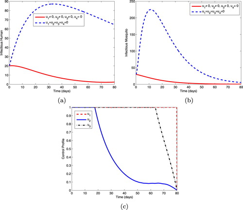
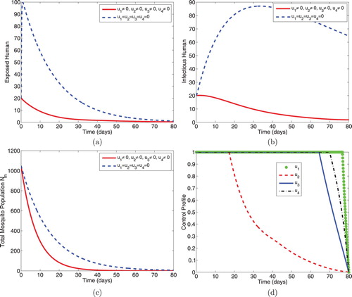
5.1.1. Intervention A: optimal use of ITNs, prophylaxis and treatment

This intervention strategy combines protective effort using insecticide-treated mosquito nets (ITNs), prophylaxis for the exposed individuals and treatment for the infectious individuals. As shown in Figure 1, the magnitudes of infectious humans and infectious mosquitoes reduce more rapidly when controls are in use than the case without controls. The control profiles in Figure 1(c) reveal that the optimal use of ITNs, $u_1\left(t\right)$, is maintained at the upper bound (100%) throughout the entire time interval [0, 80] of intervention, the optimal use of control, $u_2\left(t\right)$, is at maximum coverage (100%) for 17 days before dropping gradually to the lower bound while the control, $u_3\left(t\right)$, is maintained at the upper bound for 63 days before reducing to the lower bound at the final time.

Figure 1. Simulations showing optimal use of ITNs ($u_1$), prophylaxis ($u_2$) and treatment ($u_3$).

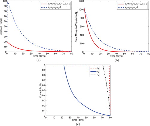
5.1.2. Intervention B: optimal use of ITNs, prophylaxis and IRS

This intervention, shown in Figure 2, combines the optimal use of insecticide-treated bednets (ITNs) $u_1\left(t\right)$, prophylaxis for the exposed humans $u_2\left(t\right)$ and vector control effort using indoor residual spraying $u_4\left(t\right)$. Figure 2(a) shows that the size of the exposed humans reduces sharply with controls. Figure 2(b) also shows the reduction in the size of the total mosquito population with controls. Optimal control profiles in Figure 2(c) show that controls $u_1\left(t\right)$, $u_2\left(t\right)$ and $u_4\left(t\right)$ should, respectively, be sustained at the maximum level till about 78 days, 22 days and 70 days before coming down to the minimum level (lower bound) in the final time.

Figure 2. Simulations depicting optimal use of ITNs ($u_1$), prophylaxis ($u_2$) and IRS ($u_4$).

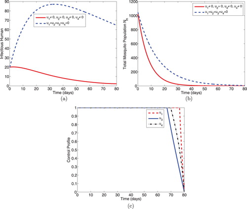
5.1.3. Intervention C: optimal use of ITNs, treatment and IRS

This strategy illustrates combined effects of personal protection effort using ITNs, treatment for the infectious individuals and vector control effort using IRS on the dynamical spread of malaria in a population. As expected, the numbers of infectious humans (Figure 3a) and total mosquito population size (Figure 3b) diminish more rapidly with controls than the case without controls. Further, Figure 3(c) reveals that controls $u_1\left(t\right)$, $u_3\left(t\right)$ and $u_4\left(t\right)$ should be maintained maximally at 100% for 76 days, 67 days and 69 days respectively, before reducing to zero in final time.

Figure 3. Simulations showing optimal use of ITNs ($u_1$), treatment ($u_3$) and IRS ($u_4$).

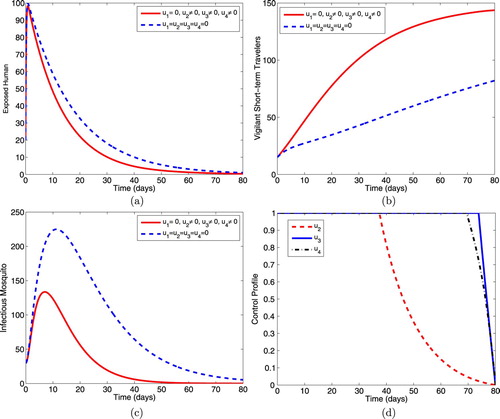
5.1.4. Intervention D: optimal use of prophylaxis, treatment and IRS

This intervention illustrates the effects of the optimal use of prophylaxis for the exposed humans, treatment for the infectious humans and the use of indoor residual spraying on the spread of malaria dynamics in the population. Figure 4(a) shows that the controls decrease the size of the exposed individuals more rapidly than when controls are not applied. Figure 4(b) shows a corresponding increase in the size of the short-term travellers who are protected against malaria infection when controls are in optimal use. Moreover, the size of the total mosquito population reduces more with controls than the size without controls (Figure 4 c). The control profile in Figure 4(d) shows that controls $u_2\left(t\right)$, $u_3\left(t\right)$ and $u_4\left(t\right)$ should be sustained at the upper bounds until 37 days, 73 days and 69 days respectively, before dropping to zero in final time.

Figure 4. Simulations depicting optimal use of prophylaxis ($u_2$), treatment ($u_3$) and IRS ($u_4$).

5.1.5. Intervention E: ITNs, prophylaxis, treatment and IRS

This intervention strategy uses the four controls $u_1\left(t\right)$, $u_2\left(t\right)$, $u_3\left(t\right)$ and $u_4\left(t\right)$ to minimize the spread of malaria governed by model (1(1) $\begin{array}{rl}\frac{\mathrm{d}{S}_h}{\mathrm{d}t}& =(1-\tau ){\mathrm{\Lambda }}_h-(1-u_1(t\left)\right)b{\text{β}}_h{S}_h\left(t\right)I_m\left(t\right)-{\mu }_h{S}_h\left(t\right)+\epsilon R_h\left(t\right)\\ \frac{\mathrm{d}{E}_h}{\mathrm{d}t}& =(1-u_1(t\left)\right)b{\text{β}}_h{S}_h\left(t\right)I_m\left(t\right)-({\alpha }_h+\varphi u_2(t)+{\mu }_h)E_h\left(t\right)\\ \frac{\mathrm{d}{I}_h}{\mathrm{d}t}& ={\alpha }_h{E}_h\left(t\right)-(\theta +\gamma u_3(t)+{\mu }_h)I_h\left(t\right)\\ \frac{\mathrm{d}{R}_h}{\mathrm{d}t}& =\varphi u_2\left(t\right)E_h\left(t\right)+(1-\delta )(\theta +\gamma u_3(t\left)\right)I_h\left(t\right)-(\sigma +\epsilon +{\mu }_h)R_h\left(t\right)\\ \frac{\mathrm{d}{V}_h}{\mathrm{d}t}& =\tau {\mathrm{\Lambda }}_h+\delta (\theta +\gamma u_3(t\left)\right)I_h\left(t\right)+\sigma R_h\left(t\right)-{\mu }_h{V}_h\left(t\right)\\ \frac{\mathrm{d}{S}_m}{\mathrm{d}t}& =(1-u_4(t\left)\right){\mathrm{\Lambda }}_m-(1-u_1(t\left)\right)b{\text{β}}_m{S}_m\left(t\right)I_h\left(t\right)-({\mu }_m+k{u}_4(t\left)\right)S_m\left(t\right)\\ \frac{\mathrm{d}{E}_m}{\mathrm{d}t}& =(1-u_1(t\left)\right)b{\text{β}}_m{S}_m\left(t\right)I_h\left(t\right)-({\alpha }_m+{\mu }_m+k{u}_4(t\left)\right)E_m\left(t\right)\\ \frac{\mathrm{d}{I}_m}{\mathrm{d}t}& ={\alpha }_m{E}_m\left(t\right)-({\mu }_m+k{u}_4(t\left)\right)I_m\left(t\right).\end{array}$(1) ). The sizes of exposed humans, infectious humans and total mosquito population decrease more sharply when controls are in use than the case when controls are not used. Figure 5(d) reveals that the optimal use of ITNs, $u_1\left(t\right)$, is maximum at 100% for 76 days before reaching the minimum in final time. Optimal use of prophylaxis, $u_2\left(t\right)$, is maintained at the maximum coverage (100%) for 17 days until it gradually reaches the lower bound in final time. Optimal use of treatment $u_3\left(t\right)$ and IRS $u_4\left(t\right)$, respectively, are kept at maximum level for 64 days and 70 days before reaching the minimum at the final time.

Figure 5. Simulations showing optimal use of ITNs ($u_1$), prophylaxis ($u_2$), treatment ($u_3$) and IRS ($u_4$).

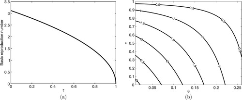
Moreover, the simulation of the autonomous system (2(2) $\begin{array}{rl}\frac{\mathrm{d}{S}_h}{\mathrm{d}t}& =(1-\tau ){\mathrm{\Lambda }}_h-b{\text{β}}_h{S}_h\left(t\right)I_m\left(t\right)-{\mu }_h{S}_h\left(t\right)+\epsilon R_h\left(t\right)\\ \frac{\mathrm{d}{E}_h}{\mathrm{d}t}& =b{\text{β}}_h{S}_h\left(t\right)I_m\left(t\right)-({\alpha }_h+{\mu }_h)E_h\left(t\right)\\ \frac{\mathrm{d}{I}_h}{\mathrm{d}t}& ={\alpha }_h{E}_h\left(t\right)-(\theta +{\mu }_h)I_h\left(t\right)\\ \frac{\mathrm{d}{R}_h}{\mathrm{d}t}& =(1-\delta )\theta I_h\left(t\right)-(\sigma +\epsilon +{\mu }_h)R_h\left(t\right)\\ \frac{\mathrm{d}{V}_h}{\mathrm{d}t}& =\tau {\mathrm{\Lambda }}_h+\delta \theta I_h\left(t\right)+\sigma R_h\left(t\right)-{\mu }_h{V}_h\left(t\right)\\ \frac{\mathrm{d}{S}_m}{\mathrm{d}t}& ={\mathrm{\Lambda }}_m-b{\text{β}}_m{S}_m\left(t\right)I_h\left(t\right)-{\mu }_m{S}_m\left(t\right)\\ \frac{\mathrm{d}{E}_m}{\mathrm{d}t}& =b{\text{β}}_m{S}_m\left(t\right)I_h\left(t\right)-({\alpha }_m+{\mu }_m)E_m\left(t\right)\\ \frac{\mathrm{d}{I}_m}{\mathrm{d}t}& ={\alpha }_m{E}_m\left(t\right)-{\mu }_m{I}_m\left(t\right).\end{array}$(2) ) showing the relationship between the basic reproduction number ${\mathcal{R}}_0$ and the protected fraction τ of human recruitment is performed in Figure 6(a), where it can be seen that $\frac{\mathrm{\partial }{\mathcal{R}}_0}{\mathrm{\partial }\tau }<0$ as established in (6(6) $\frac{\mathrm{\partial }{\mathcal{R}}_0}{\mathrm{\partial }\tau }=-{\left(\frac{2(\theta +{\mu }_h)({\alpha }_h+{\mu }_h)({\alpha }_m+{\mu }_m){\mu }_m^2{\mu }_h}{b^2{\text{β}}_h{\alpha }_h{\text{β}}_m{\alpha }_m(1-\tau ){\mathrm{\Lambda }}_h{\mathrm{\Lambda }}_m}\right)}^{-1/2}<0.$(6) ). This confirms that as τ increases through the interval $0\le \tau \le 1$, the spread of malaria in the population decreases. Figure 6(b) is the contour plot of the basic reproduction number ${\mathcal{R}}_0$ as a function of two parameters, namely the fraction of human recruitment who are protected travellers (τ) and spontaneous recovery rate of infectious humans (θ). It is observed that increasing the values τ and θ has the capacity to reduce the value of ${\mathcal{R}}_0$ to a value less than unity and hence reduce the spread of malaria in the community.

Figure 6. Simulation showing relationship between ${\mathcal{R}}_0$ and τ with 2D-Contour plot of ${\mathcal{R}}_0$ as a function of τ and θ.

5.2. Cost-effectiveness analysis

To determine the most cost-effective strategy of all the various combinations of the intervention strategies considered in this work, the incremental cost-effectiveness ratio (ICER) is calculated following the approach used in [2, 6, 17, 28]. ICER is usually employed to measure up the changes between the costs and health benefits of any two different intervention strategies competing for the same limited resources. Hence, this ICER is simply defined as the ratio of change in total cost to the change in control benefits. $\mathrm{I}\mathrm{C}\mathrm{E}\mathrm{R}=\frac{\mathrm{c}\mathrm{h}\mathrm{a}\mathrm{n}\mathrm{g}\mathrm{e}\mathrm{i}\mathrm{n}\mathrm{t}\mathrm{o}\mathrm{t}\mathrm{a}\mathrm{l}\mathrm{c}\mathrm{o}\mathrm{s}\mathrm{t}}{\mathrm{c}\mathrm{h}\mathrm{a}\mathrm{n}\mathrm{g}\mathrm{e}\mathrm{i}\mathrm{n}\mathrm{c}\mathrm{o}\mathrm{n}\mathrm{t}\mathrm{r}\mathrm{o}\mathrm{l}\mathrm{b}\mathrm{e}\mathrm{n}\mathrm{e}\mathrm{f}\mathrm{i}\mathrm{t}\mathrm{s}}.$ The ICER numerator includes the differences in intervention costs, averted disease costs and costs of prevented cases among others. While the ICER denominator measures the difference in health outcome, which includes the total population of infection averted or total number of cases of susceptibility prevented as the case may be.

Based on the simulation results of the optimality system, the control intervention strategies: A (which combines ITNs ($u_1$), prophylaxis ($u_2$) and treatment ($u_3$)), B (which combines ITNs ($u_1$), prophylaxis ($u_2$) and IRS ($u_4$)), C (which combines ITNs ($u_1$), treatment ($u_3$) and IRS ($u_4$)), D (which combines prophylaxis ($u_2$), treatment ($u_3$) and IRS ($u_4$)) and E (which combines ITNs ($u_1$), prophylaxis ($u_2$), treatment ($u_3$) and IRS ($u_4$)) are ranked in increasing order of total number of infection averted given in Table 3.

Table 3. Increasing order of infections averted.

Intervention	Total infections	Total costs ($)	ICER
strategies	averted
A	0.0491	143,560	2,923,828.9
D	42.6737	189,790	1084.6
B	43.3423	111,850	–
C	43.3423	114,120	–
E	43.3423	167,030	–

To compare intervention strategies A and D incrementally, the ICER for the two competing strategies is calculated as follows: $\begin{array}{rl}\mathrm{I}\mathrm{C}\mathrm{E}\mathrm{R}\left(\mathrm{A}\right)& =\frac{143,560}{0.0491}=2,923,828.9\\ \mathrm{I}\mathrm{C}\mathrm{E}\mathrm{R}\left(\mathrm{D}\right)& =\frac{189,790-143,560}{42.6737-0.0491}=\mathrm{1084.6.}\end{array}$ It can be seen that ICER (A) > ICER (D). This implies that strategy A is more costly and less effective than strategy D. Hence, strategy A is excluded from the list of alternative interventions and ICER is recalculated for strategies D and B as shown in Table 4. Since ICER (D) > ICER (B), it follows that strategy D is strongly dominated, more costly and less effective when compared with strategy B. Hence, the intervention strategy D is excluded from the list of alternative interventions. At this juncture, it is needless to recalculate ICER further since it can be observed that the remaining intervention strategies B, C and E avert the same total number of infections. However, strategy B requires least cost when compared with strategies C and E. Therefore, intervention strategy B is considered the most cost effective among the strategies analysed in this study.

Table 4. Comparison between interventions D and B.

Intervention	Total infections	Total costs ($)	ICER
strategies	averted
D	42.6737	189,790	4447.5
B	43.3423	111,850	$-116,571.9$
C	43.3423	114,120	–
E	43.3423	167,030	–

6. Conclusion

This work is concerned with the mathematical analysis of a malaria transmission model with naturally acquired immunity in the presence of protected travellers. The model is shown to exhibit the phenomenon of backward bifurcation where the stable malaria-free and malaria-present steady states coexist as the basic reproduction number crosses unity. The existence of backward bifurcation exhibited by the formulated model is caused by the presence of the transient acquired natural immunity.

To control the spread of malaria in a population, multiple time-dependent optimal control variables, including personal protection using ITNs; prophylaxis for latently infected (exposed) humans; treatment of infectious humans and vector control using indoor residual spray (IRS) are considered. Theoretical analysis of the optimal control model is carried out and the model is simulated to investigate the effects of combining at least any three of the control intervention strategies on the spread dynamics of malaria in the community. It is shown that the sizes of infected humans and the total mosquito population are minimized by the various combinations of the control variables.

However, the cost-effectiveness analysis carried out shows that the combination of the optimal use of ITNs, prophylaxis and IRS is the most cost-effective intervention strategy of all the various combinations of the controls considered in this work. Therefore, using all the control strategies as suggested in [32] is not advisable when the available resources are limited. Further simulations show that with an increased fraction of protected travellers, the basic reproduction number is reduced significantly. This indicates that the presence of protected travellers in a population does not constitute threat to the control of malaria transmission but rather assists in curbing further spread of the disease in the population.

Acknowledgement

The authors would like to thank Vaal University of Technology for the provided support. Improvement of the original manuscript is due largely to the constructive comments of reviewers and handling editor.

Disclosure statement

No potential conflict of interest was reported by the author(s).

ORCID

S. Olaniyi  http://orcid.org/0000-0001-6492-1405

Additional information

Funding

Okosun is supported by the National Research Foundation (NRF), South Africa, under Grant numbers 115029 and 115524.

References

- F.B. Agusto and J.M. Tchuenche, Control strategies for the spread of malaria in humans with variable attractiveness, Math. Popul. Stud. 20(2) (2013), pp. 82–100. doi:10.1080/08898480.2013.777239
- J.O. Akanni, F.O. Akinpelu, S. Olaniyi, A.T. Oladipo and A.W. Ogunsola, Modelling financial crime population dynamics: optimal control and cost-effectiveness analysis, Int. J. Dynam. Control (2019), pp. 1–14. doi:10.1007/s40435-019-00572-3
- J.K. Asamoah, F.T. Oduro, E. Bonyah and B. Seidu, Modelling of rabies transmission dynamics using optimal control analysis, J. Appl. Math. 2017 (2017), pp. 1–23. Article ID 2451237. doi:10.1155/2017/2451237
- S. Athithan and M. Ghosh, Stability analysis and optimal control of a malaria model with larvivorous fish as biological control agent, Appl. Math. Inf. Sci. 9(4) (2015), pp. 1893–1913. doi:10.12785/amis/090428
- E.A. Bakare and C.R. Nwozo, Effect of control strategies on the optimal control analysis of a human-mosquito model for malaria under the influence of infective immigrants, Int. J. Math. Comput.26(1) (2015), pp. 51–73.
- H.W. Berhe, O.D. Makinde and D.M. Theuri, Optimal control and cost-effectiveness analysis for dysentery epidemic model, Appl. Math. Inf. Sci. 12(6) (2018), pp. 1183–1195. doi:10.18576/amis/120613
- K. Blayneh, Y. Cao and H. Kwon, Optimal control of vector-borne diseases: Treatment and prevention, Discrete Contin. Dyn. Syst. Ser. B. 11(3) (2009), pp. 587–611. doi:10.3934/dcdsb.2009.11.587
- C. Castillo-Chavez and B. Song, Dynamical models of tuberculosis and their applications, Math. Biosci. Eng. 1(2) (2004), pp. 361–404.
- N. Chitnis, J.M. Cushing and J.M. Hyman, Bifurcation analysis of a mathematical model for malaria transmission, SIAM J. Appl. Math. 67(1) (2006), pp. 24–45.
- B. Dembele and A. Yakubu, Optimal treated mosquito bed nets and insecticides for eradication of malaria in Missira, Discrete Contin. Dyn. Syst. Ser. B. 14(6) (2012), pp. 1831–1840. doi:10.3934/dcdsb.2012.17.1831
- A.O. Egonmwan and D. Okuonghae, Analysis of a mathematical model for tuberculosis with diagnosis, J. Appl. Math. Comput. 59 (2019), pp. 129–162. doi:10.1007/s12190-018-1172-1
- F. Fatmawati, W. Windarto and L. Hanif, Application of optimal control strategies to HIV-malaria co-infection dynamics, J. Phys. Conf. Ser. 974 (2018), pp. 1–15. doi:10.1088/1742-6596/974/1/012057
- W.H. Fleming and R.W. Richel, Deterministic and Stochastic Optimal Control, Springer, New York, 1975.
- H.E. Gervas, N.K. Opoku and S. Ibrahim, Mathematical modelling of human African trypanosomiasis using control measures, Comput. Math. Methods Med. 2018 (2018), pp. 1–13. Article ID 5293568. doi:10.1155/2018/5293568
- H.W. Hethcote, The mathematics of infectious diseases, SIAM Rev. 42(4) (2000), pp. 599–653.
- R.E. Howes, R.C. Reiner Jr., K.E. Battle, Plasmodium vivax transmission in Africa. PLoS Negl. Trop. Dis. 9(11) (2015), p. e0004222). . .doi:10.1371/journal.pntd.0004222.
- A. Hugo, O.D. Makinde, S. Kumar and F.F. Chibwana, Optimal control and cost effectiveness analysis for Newcastle disease eco-epidemiological model in Tanzania, J. Biol. Dyn. 11(1) (2017), pp. 190–209. doi:10.1080/17513758.2016.1258093
- O. Koutou, B. Traoré and B. Sangaré, Mathematical modeling of malaria transmission global dynamics: taking into account the immature stages of the vectors, Adv. Differ. Eq. 2018 (2018), pp. 1–34. doi:10.1186/s13662-018-1671-2
- A.A. Lashari, M. Ozair, G. Zaman and X. Xuezhi, Global analysis of a host-vector model with infectious force in latent and infected period, Acta Anal. Funct. Appl. 14(4) (2012), pp. 321–329. doi:10.3724/SP.J.1160.2012.00321
- S. Lenhart and J.T. Workman, Optimal Control Applied to Biological Models, London, Chapman & Hall, 2007.
- T.M. Malik, A.A. Alsaleh, A.B. Gumel and M.A. Safi, Optimal strategies for controlling the MERS coronavirus during a mass gathering, Glob. J. Pure Appl. Math. 11(6) (2015), pp. 4831–4865.
- C. Modnak, Mathematical modelling of an avian influenza: optimal control study for intervention strategies, Appl. Math. Inf. Sci. 11(4) (2017), pp. 1049–1057. doi:10.18576/amis/110411
- P.M. Mwamtobe, S. Abelman, J.M. Tchuenche and A. Kasambara, Optimal (control of) intervention strategies for malaria epidemic in Karonga district, Malawi, Abst. Appl. Anal. 2014 (2014), pp. 1–20. Article ID 594256. doi:10.1155/2014/594256
- O.S. Obabiyi and S. Olaniyi, Asymptotic stability of malaria dynamics with vigilant human compartment, Int. J. Appl. Math. 29(1) (2016), pp. 127–144. doi:10.12732/ijam.v29i1.10
- S.I. Oke, M.B. Matadi and S.S. Xulu, Optimal control analysis of a mathematical model for breast cancer, Math. Comput. Appl. 23(21) (2018), pp. 1–28. doi:10.3390/mca23020021
- K.O. Okosun, M.A. Khan, E. Bonyah and S.T. Ogunlade, On the dynamics of HIV-AIDS and cryptosporidiosis, Eur. Phys. J. Plus. 132 (2017), p. 363. doi:10.1140/epjp/i2017-11625-3
- K.O. Okosun and O.D. Makinde, A co-infection model of malaria and cholera diseases with optimal control, Math. Biosci. 258 (2014), pp. 19–32. doi:10.1016/j.mbs.2014.09.008
- K.O. Okosun, O. Rachid and N. Marcus, Optimal control strategies and cost-effectiveness analysis of a malaria model, BioSyst. 111 (2013), pp. 83–101. doi:10.1016/j.biosystems.2012.09.008
- S. Olaniyi and O.S. Obabiyi, Qualitative analysis of malaria dynamics with nonlinear incidence function, Appl. Math. Sci. 8(78) (2014), pp. 3889–3904. doi:10.12988/ams.2014.45326
- S. Olaniyi, M.A. Lawal and O.S. Obabiyi, Stability and sensitivity analysis of a deterministic epidemiological model with pseudo-recovery, IAENG Int. J. Appl. Math. 46(2) (2016), pp. 160–167.
- S. Olaniyi, Dynamics of Zika virus model with nonlinear incidence and optimal control strategies, Appl. Math. Inf. Sci. 12(5) (2018), pp. 969–982. doi:10.18576/amis/120510
- S. Olaniyi, K.O. Okosun, S.O. Adesanya, Global stability and optimal control analysis of malaria dynamics in the presence of human travelers. Open Infect. Dis. J. 10 (2018), pp. 166–186. doi:10.2174/1874279301810010166
- M.A. Osman and I.K. Adu, Simple mathematical model for malaria transmission, J. Adv. Math. Comput. Sci. 25(6) (2017), pp. 1–24. doi:10.9734/JAMCS/2017/37843
- L.S. Pontryagin, V.G. Boltyanskii, R.V. Gamkrelidze and E.F. Mishchenko, The Mathematical Theory of Optimal Processes, Wiley, New York, 1962.
- C.R. Rector, S. Chandra and J. Dutta, Principles of Optimization Theory, Narosa Publishing House, New Delhi, 2005.
- J.P. Romero-Leiton, J.M. Montoya-Aguilar and E. Ibargüen-Mondragón, An optimal control problem applied to malaria disease in Colombia, Appl. Math. Sci. 12(6) (2018), pp. 279–292. doi:10.12988/ams.2018.819
- R. Ross, The Prevention of Malaria, London, John Murray, 1911.
- A.K. Srivastav, N.K. Goswami, M. Ghosh and X-Z. Li, Modeling and optimal control analysis of Zika virus with media impact, Int. J. Dyn. Control. 6 (2018), pp. 1673–1689. doi:10.1007/s40435-018-0416-0
- P. van den Driessche and J. Watmough, Reproduction numbers and sub-threshold endemic equilibria for compartmental models of disease transmission, Math. Biosci. 180 (2002), pp. 29–48. doi:10.1016/S0025-5564(02)00108-6
- WHO, World Malaria Report, Geneva, World Health Organization Press, 2015.
- WHO, World Malaria Report, Geneva, World Health Organization Press, 2018.