
 ?Mathematical formulae have been encoded as MathML and are displayed in this HTML version using MathJax in order to improve their display. Uncheck the box to turn MathJax off. This feature requires Javascript. Click on a formula to zoom.
Abstract
In Nature, species coexistence is much more frequent than what the classical competition model predicts, so that scientists look for mechanisms that explain such a coexistence. We revisit the classical competition model assuming that individuals invest time in competing individuals of the other species. This assumption extends the classical competition model (that becomes a particular case of the model presented) under the form of a Holling type II term, that we call competitive response to interfering time. The resulting model expands the outcomes allowed by the classical model by (i) enlarging the range of parameter values that allow coexistence scenarios and (ii) displaying dynamical scenarios not allowed by the classical model: namely, bi-stable conditional coexistence in favour of i (either species coexist or species i wins) or tri-stable conditional coexistence (either species coexist or any of them goes extinct), being exclusion in both cases due to priority effects.
1. Introduction
The structure of ecosystems is determined by the interaction between biotic and abiotic elements. Species competition is among the most important biotic factors; individuals compete almost everywhere with individuals of the same species (intra-species competition) and/or individuals of a different species (inter-species competition).
The early theory of competition spinned around the works of Lotka, Volterra and Gause. Namely, Lotka and Volterra [Citation23,Citation35] found that coexistence is possible when intra-species competition is stronger than inter-species competition. The Competitive exclusion principle set by Gause [Citation13] stated that two species occupying the same niche cannot coexist [Citation15]. This theoretical framework is at odds with reality, given that species coexist much more often than expected within this framework [Citation30,Citation33,Citation36].
Different explanations and mechanism have been proposed to explain why species coexistence is more prevalent than species exclusion. From the above referred framework, that means to describe mechanisms reducing inter-species competition (see [Citation38] and references quoted there). For instance, in [Citation2] extensions of the competitive exclusion principle were proposed. The classical niche theory [Citation21,Citation24] assumes that differences among two species in the use of available resource types entail a reduction in the per capita competitive effects of the two species on each other. Species dispersal strategies and habitat heterogeneity [Citation3,Citation25,Citation29], the resolution at which resources are perceived by each competing species [Citation33], the so-called equalizing and stabilizing mechanisms (a trend to minimize in average differences in species fitness or to increase negative intra-specifies interactions relative to negative inter-species interactions, respectively) [Citation10], host-specific pets-based mechanism [Citation8,Citation16,Citation37] or age-structure and distance between colonies [Citation6].
The above-mentioned mechanisms focus on species strategies or environmental constrains. An alternative approach consists on focusing on the actual way competition takes place. Despite of its importance, the classical Lotka–Volterra model was somehow oversimplifying. This model assumes that species are perfectly mixed and that the effect of one species on the other is linear to the population size of its competitor [Citation30,Citation38]. However, [Citation5,Citation34] empirically shown that competitive effects can be density-dependent which entails that the nullclines, the zero growth curves of the corresponding differential or difference equations system, are non-linear in contrast to the linear nullclines of the classical Lotka–Volterra competition model. Subsequently, Nunney [Citation30] argued that it is more interesting to focus on the nullclines curvature rather than on getting accurate estimates of the classical competition parameters model. He proposed a general model formulation in terms of the so-called resource availability functions and proved that the curvature of such a functions determine the curvature of the model nullclines. In contrast to predator–prey models [Citation7,Citation11,Citation12,Citation17,Citation32], most of the other variations of the classical model are phenomenological as in [Citation5,Citation34] (and references citing these papers), but also justifying the form of the species interference term based on ‘food encounters’ [Citation31] on available resources [Citation14] or on a cooperation–competition mechanism [Citation38]. Also in [Citation1,Citation27] an elaborated social model is proposed, in which the individuals of one population gather together in herds, while the other one shows a more individualistic behaviour, so that interactions among the two populations occur mainly through the perimeter of the herd.
The departure assumption in this work is that competing takes time rather than being instantaneous. In other words, two individuals of different species that compete for a given resource do need to invest certain amount of time to get this resource. The model presented herein extends the classical interference competition model [Citation13] (see also [Citation4]) that becomes a particular case when competition is assumed to be instantaneous. The mechanism is essentially that used in Holling works [Citation17,Citation18]. Indeed, the interference term of the model takes the form of a Holling type II term [Citation17] that we call Holling type II competitive response to interference time.
As a result, we found a range of parameter values that leads to the same competition outcomes as in the classical model. In addition, we have found also competition outcomes not allowed by the classical model. In the so-called bi-stable conditional coexistence (in favour of one of the species) either species coexist or one of them goes extinct, depending on the initial number of individuals (i.e. due to priority effects). There is also the so-called tri-stable conditional coexistence scenario that allows either species coexistence or any of them to go extinct due to priority effects.
The manuscript is organized as follow: in Section 2, we derive the above-mentioned model. We also analyze there those scenarios that are the same as in the classical model. In Section 3, we gain an insight on the role of the competitive response by considering that only individuals of one species expend time in competition. In Section 4, we consider the complete model with competitive response on both species. The system can be analytically analyzed under the assumptions of either symmetric (Section 4.1) or asymmetric (Section 4.2) competition. These results are completed in Section 4.3 with numerical simulations on the most general model. Finally, Section 5 is devoted to the discussion of results and to drawn conclusions.
2. The Holling type II competition model
The departure model is the classical Lotka–Volterra competition model
(1)
(1) where
and
stand for the amount of individuals and the intrinsic growth rate of species i = 1, 2, respectively. Coefficients
account for intra (i = j) and inter (
) species competition, for i, j = 1, 2.
The key assumption of the classical model (Equation1(1)
(1) ) is that the per capita growth rate of species i decreases linearly with
and
(
), i.e.
In particular, it means that given a fixed number of individuals of species j, the competitive pressure that species
exerts over species i increases as the number of individuals of species i increases. This assumption may not always make sense on interference competition if competing takes time, since a fixed number of individuals of species j can not interfere the same on species i when competing with, lets say, 10 or 1000 individuals of species i.
We propose an alternative formulation that is an adaptation of [Citation17,Citation18] to the current context. As in [Citation17], we assume that the probability of a given individual of species i to encounter an individual of species within a fixed time interval T (in a fixed region) depends linearly on the number of individuals of species j. Then, the number
of competitors of species
that become extinct due to the interference of a single individual of species
is given by
where
is the total amount of individuals of species i,
stands for the time that individuals are active (searching for/defending resources or territories, matching,…), a is the product of the resources finding rate times the probability of meeting a competitor; thus a is a constant equivalent to Holling's discovery rate. If interference does not take time,
; otherwise
. Let
be the average time that interference takes, so that
, that implies
that is equivalent to
(2)
(2) that we call Holling type II competitive response to interference time. Plugging this expression in system (Equation1
(1)
(1) ) and relabelling coefficients yields
(3)
(3) Thus, the inter-species competition coefficient is constant only in case of instantaneous interactions (i.e.
due to
). Otherwise, the impact of species j on species i is density dependent, a decreasing function of
for a fixed amount of individuals of species j.
Note that in general , since the searching rates, the probabilities of finding other species' competitors or the time spent competing/snatching resources can be different for each species due to phenotypical and/or behavioural traits.
Also, in this work we focus on mechanisms that facilitate species coexistence. Thus, even if it could make sense, we do not consider the effect of the time elapsed when competing with conspecifics. Doing so we stress the inter-species dynamics and avoid possible compensatory effects (of the time invest in intra/inter-species competition) that are beyond the scope of this work.
In the sequel, we analyze system (Equation3(3)
(3) ) and compare the competition outcomes to those yield by the classical competition model (Equation1
(1)
(1) ). Let us first rewrite system (Equation3
(3)
(3) ) in a suitable way by setting
,
and
, that yields
(4)
(4) Note that the competitive strength
is the ration of the inter-species and intra-species dynamics rates. Also,
is the ratio of the capability of endure competitors (meaning that the larger is
, the more time needs a competitor to make species i surrender) and the intra-species competition rates.
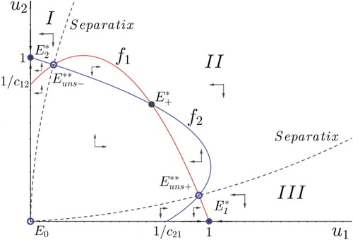
For the convenience of the reader, we recall the possible outcomes of the classical competition model, that are summarized in Figure :
Figure 1. Top panel: possible phase portraits of the classical competition system (system (Equation4(4)
(4) )) with
). Bottom panel: species competition outcomes as function of the competitive strength
and
.
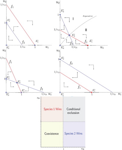
Theorem 2.1
Consider system (Equation4(4)
(4) ) with
. Then, for any solution with initial values in the positive cone
is globally asymptotically stable if, and only if
The equilibrium point
Proof.
See Section 3.5 in .
Conditions in Theorem 2.1 state ,
, as a threshold value to compare with the competitive strength
,
. In short, species j can not drive species i to extinction if, and only if, the competitive strength
,
, of species j on species i is less than 1 (see Figure for a graphical summary).
We next show that system (Equation4(4)
(4) ) is well behaved, in the sense of the following proposition:
Theorem 2.2
Consider system (Equation4(4)
(4) ). Then,
The axes are forward invariant.
The solutions are bounded from above.
The positive cone
Proof.
Statement 1 follows from the fact that any solution with initial values on one the (say) axes, fulfills an uncoupled system that consists of the logistic equation
and
. Regarding 2, any solution of equation i is bounded from above by the solutions of the logistic equation
, i = 1, 2. The third item is consequence of 1 and 2.
The following result establishes the existence and stability properties of the so-called trivial and semi-trivial equilibrium points of system (Equation4(4)
(4) ), that is the same as in the classical model. From now on, we assume that
for i = 1, 2.
Theorem 2.3
Consider system (Equation4(4)
(4) ). Then,
The trivial equilibrium point
There exist semi-trivial equilibrium points
Proof.
The existence of , i = 0, 1, 2, follows from direct calculations. The stability conditions follow from an standard analysis of the eigenvalues of the Jacobian matrix.
The next sections are devoted to understand the effect on the competition outcome of considering a Holling type II competition term in just one species.
3. Holling type II response on just one species
In order to gain an insight on the role of the competitive response, we first assume that only species 2 spends time when competing species 1. Thus, we analyze system
(5)
(5) System (Equation5
(5)
(5) ) is a particular case of system (Equation4
(4)
(4) ), so that we already know that it is well behaved. Proposition 2.3 also holds in relation to the existence and local stability of the trivial and semi-trivial equilibrium points.
In the sequel, we focus on the non-trivial equilibrium points. Note that the nullcline that solves
is either
or an oblique straight line, as in the classical model. In contrast, the nullcline
that solves
is either
or a parabola. This feature is behind the differences between the outcomes of the classical model and system (Equation5
(5)
(5) ), see Figure and note that panel (v) leads to a dynamical scenario that is not covered by the classical system (see Figure ).
Figure 2. Possible phase portrait of system (Equation5(5)
(5) ).
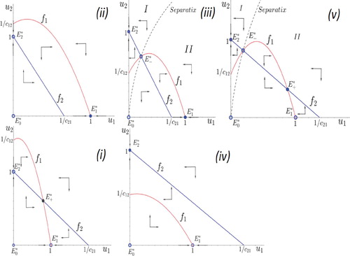
Indeed, Figure suggest that most of the outcomes (4 over 5) of system (Equation5(5)
(5) ) are qualitatively the same as in the classical model. The following result displays conditions that describe those scenarios.
Theorem 3.1
Consider system (Equation5(5)
(5) ). Then, for any solution with initial values in the positive cone:
Assume now that
Assume that
Note that conditions in statements (1)–(4) avoid (i) the case of two interior equilibrium points (see Figure (v)) and (ii) the case of tangent nullclines in the first quadrant (see Figure ).
Figure 3. Phase portrait related to tangent nullclines. Solid points denote the locally asymptotically stable equilibrium points and
while the equilibrium
is non-stable.
Proof.
Consider the nullclines associated to the flow of system (Equation5(5)
(5) ) defined by
that is, a parabola and a straight line (see Figure ) so that the non-trivial equilibrium points are the solutions to the second degree equation resulting from
, that is
(9)
(9) As for statement (1), being
globally asymptotically stable implies that there is no interior equilibrium points on the positive cone. Thus, either
for all
(that is,
and
and nullclines meet outside the positive cone) or condition (Equation6
(6)
(6) ) holds (that is equivalent to the discriminant of the solution of Equation (Equation9
(9)
(9) ) being negative and nullclines do not meet). However condition (Equation6
(6)
(6) ) needs
, which implies (by linearization) that
is unstable that is a contradiction with the departure hypothesis, so that
and
holds. Conversely, assume that
and
. Then, analyzing the phase portrait as in [Citation4] yields the global stability of
.
Regarding statement 2, we have already said that condition (Equation6(6)
(6) ) is equivalent to the discriminant of the solution of Equation (Equation9
(9)
(9) ) being negative. That is to say that
and
do not meet anywhere which, given the geometry of the nullclines, yields the global stability of
.
The remaining statements follow mutatis mutandi the proof of the corresponding results for classical competition model; see, for instance, [Citation4] or .
We turn our attention to these settings that lead to new dynamical scenarios with respect to those displayed by the classical system. It will turn out that the following curve, that results from equating to zero the discriminant of the solution of Equation (Equation9(9)
(9) ) and solving the resulting equation on
, plays a key role.
Lemma 3.2
Consider the function
(10)
(10) then,
is an unimodal function such that
For
The maximum is reached at
Proof.
It follows from direct calculations.
In the following result, we assume that and
, so that in the classical model species 2 wins regardless of the initial number of individuals of each species. Then, if the species 1 competitive ability is not too small so that
, then species may either coexist or species 2 win unconditionally, depending on initial values, what we call bi-stable conditional coexistence in favour of species 1. Otherwise, species 2 wins always.
Theorem 3.3
Consider system (Equation5(5)
(5) ) and assume that
and
. Then, for any solution with initial values in the positive cone:
The condition
Assume now that
Assume now that
Assume now that
If condition
Proof.
Let us recall that the non-trivial equilibrium points are the solutions to Equation (Equation9
(9)
(9) ) and that
Equating to zero the discriminant of the above expression and solving the resulting equation on
yields
as defined in (Equation10
(10)
(10) ).
Condition
The discriminant in
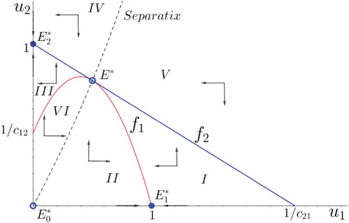
Regarding the stability, we claim that this is a degenerate case, in the sense that zero is an eigenvalue of the Jacobian matrix of the flow of system (Equation5
Besides, consider the corresponding phase portrait (see Figure ). A first claim is that regions I and III are trapping regions, meaning that any solution entering one of them cannot leave such a region. It has two consequences: on the one hand, it precludes the existence of limit cycles.
On the other hand, solutions with initial values in region I converge to
We already know that condition
Note that
Note that
It follows from the previous discussion.
So we have completed the analysis of system (Equation5(5)
(5) ). Figure summarizes the possible outcomes of system (5), that extends those allowed by the classical system (1) (see the bottom panel of Figure 1). The above results are deeply discussed in Section 5.
Figure 4. Competition outcomes of system (Equation5(5)
(5) ) as function of the competitive strengths
,
.
4. Holling type II response on both species
We turn now our attention to the complete model (Equation4(4)
(4) ). Section 3 suggests that we must expect either settings such that the classic competition model and system (Equation4
(4)
(4) ) behave qualitatively the same (and differences are, if any, in the transient time) or such that dynamics is a little bit more complicated and expands the coexistence conditions.
After Proposition 3.1, we focus on the existence and stability of the non-trivial equilibrium points. The nullclines of system (Equation4(4)
(4) ) are parabolas, defined by
(15)
(15) so that the equilibrium points are given by the solutions to the fourth degree equation
(16)
(16) where
(17)
(17) It is well known that there exists a closed formula to solve this equations but, unfortunately, its expression is too involved to get any biological insight. Then, we adopt a numerical approach to analyze system (Equation4
(4)
(4) ). However, there are two ecologically meaningful scenarios, symmetric and asymmetric competition [Citation39], that lead to simplifications in (Equation17
(17)
(17) ) that allow an analytic study that we address next.
4.1. Symmetric competition and Holling type II competitive response
Symmetric competition takes place, for instance, between individuals of different species with similar phenotypic traits [Citation39]. This idea can be translated to system (Equation4(4)
(4) ) by setting the model coefficients as
(18)
(18) see [Citation22]. In such a case, coefficients (Equation17
(17)
(17) ) specialize into
(19)
(19) It turns out that c = 1 and
are candidate to be threshold values for the behaviour of the model (for instance, think of Descartes' Rule). We first claim that the nullclines are symmetric with respect to the
line, namely
Lemma 4.1
Consider the nullcline curves (Equation15(15)
(15) ) with coefficients (Equation18
(18)
(18) ), so that
are symmetrical with respect to the straight line
, meaning that they are reciprocal functions
As a consequence, there exists two equilibrium points on the
line with coordinates
(20)
(20) where
is in the positive cone while
is in the third quadrant.
Proof.
It follows from direct calculations.
The following proposition describes the dynamics of the model under symmetric competition and includes a tri-stability conditional coexistence scenario that is not allowed by the classical model (see Figure ).
Figure 5. Phase portrait in the symmetric competition scenario that displays the tri-stability conditional coexistence outcome.
Theorem 4.2
Consider system (Equation4(4)
(4) ) along with the symmetry conditions
and
. Then
For any
Assume now that
For any
For any
Proof.
Let us recall that system (Equation4(4)
(4) ) possesses, at most, four equilibrium points and lemma 4.1 yields the expression of two of them.
We will show that
Dividing
For any
Direct calculations show that
4.2. Asymmetric competition and Holling type II competitive response
Asymmetric competition [Citation20] takes place, for instance, between individuals of different species with dissimilar phenotypic traits [Citation39]. We impose the following constraints to the model coefficients ,
and
,
, in order to set full asymmetric competition. Thus, coefficients (Equation17
(17)
(17) ) become
(22)
(22) As before, c = 1 and
are candidates to be a threshold value for the qualitative behaviour of the solutions of system (Equation4
(4)
(4) ).
We do not perform a complete analysis of the resulting model; we just state conditions that lead to bi-stable conditional coexistence scenarios:
Theorem 4.3
Consider system (Equation4(4)
(4) ) along with the asymmetry conditions
and
. Then
For any
For any
For any
Assume now that
For any
For any
Proof.
It follows arguing as in Propositions 2.2 and 4.2.
4.3. The general case: numerical analysis
As we have already said, the equilibrium points of system (Equation4(4)
(4) ) are the roots of the 4th degree polynomial Equation (Equation16
(16)
(16) ). These solutions depend on the coefficients (Equation17
(17)
(17) ) that depend on
and
, that is, on four parameters. Close expressions exist for the roots of (Equation16
(16)
(16) ), but are so involved that we could not derive any biological information from them. We have also attempted to use Cardano's and Ferrari's theorem or Sturm's sequence, Descartes's rule and Burdan–Fourier theorem with no positive results.
Therefore, we perform a numerical analysis using an algorithm written in MatLab software. From the results found in Sections 3, 4.1 and 4.2 we decided to plot diagrams that display, for fixed values of , i = 1, 2, the number of equilibrium points and its stability for
,
ranging in a given interval, as in Figure .
As there are no analytical results for the complete model different from those already obtained at the beginning of Section 2, we left the results of the numerical experiments to the discussion and conclusions Section 5.
5. Discussion and conclusions
In this manuscript, we revisit he classical competition model (Equation1(1)
(1) ) under the assumption that interfering with competitors of other species takes time. We have found that (i) the classical competition model is a particular case of the model derived herein when interactions do not consume time, (ii) the more time interfering with competitions takes the more likely coexistence is and, indeed, (iii) the new model allows multi-stability scenarios.
Geometrically, accounting for the time spent competing bends nullclines from the straight lines found in the classical model into a parabolic shape. This feature has been previously found in [Citation30,Citation38] under different departure hypotheses and not fully analyzed (only qualitatively). Compare the nullcline of species 1 in the classical competition model (, left panel in Figure ) and in system (Equation4
(4)
(4) ) (
, central and right panels in Figure ), where
(23)
(23) Let us recall that the bounded region defined by the axes and the nullcline of species 1 defines the values of the population size of species 2 that allow species 1 to keep growing.
Figure 6. The nullcline of system (Equation4
(4)
(4) ) for increasing values of
: left,
(i.e. the classical Lotka–Volterra model (Equation1
(1)
(1) )), centre,
and right,
.
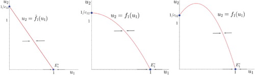
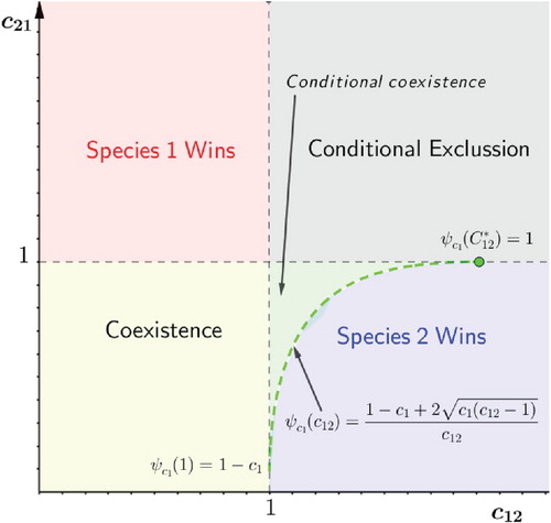
Figure 7. Competition outcomes of system (Equation5(5)
(5) ) as function of the competitive strengths
,
for increasing values of
(from left to right). The code colour is the same as in Figure except the dark blue region that represents bi-stable conditional coexistence region in favour of species 1. The boundary between the blue regions is the graph of
. The figure is based on numerical calculations (the source code is available in [Citation9]) alingment!!! and has been edited to improve it. Parameter values are
,
and, from left to right,
.
![Figure 7. Competition outcomes of system (Equation5(5) u1′=r1u1−u12−c12u1u21+c1u1u2′=r2(u2−u22−c21u1u2)(5) ) as function of the competitive strengths c12, c21 for increasing values of c1 (from left to right). The code colour is the same as in Figure 1 except the dark blue region that represents bi-stable conditional coexistence region in favour of species 1. The boundary between the blue regions is the graph of c21=ψc1(c12). The figure is based on numerical calculations (the source code is available in [Citation9]) alingment!!! and has been edited to improve it. Parameter values are 0<c12,c21<2, c2=0 and, from left to right, c1=0.3,1,1.8.](/cms/asset/7e0a60ff-e25f-48c3-b654-d7f16981304a/tjbd_a_1742392_f0007_oc.jpg)
The classical model estates that the larger is , the less tolerant is to the presence of
, meaning that as
increases,
keeps growing only if
decreases (according to the nullcline slope).
On the contrary, accounting for the time spent competing weakens of even reverses this trend, since the region below the nullcline increases with . In words, the more time species 2 needs to snatch resources to species 1, the less time has species 2 to compete with other individuals of species 1. We may say that such a time is moderate for
and large if
. Looking closer to the nullcline of
in system (Equation4
(4)
(4) ), note that achieves its maximum
at
. Then,
Condition
If
Then, is a threshold value for
to tolerate an increasing amount of individuals of species 2. Interestingly, note that
is bounded from above while
is unbounded for increasing values of
. On the one hand, that is to say that intra-species competitive pressure will show up at
, since the maximum is reached at
regardless of
. However, if
(so that
) intra-species pressure is added to inter-species pressure, although the later is slightly weaken by the little time spent competing. On the other hand,
still increases if
does so. Thus, we can somehow discriminate the tolerance to intra and inter-species crowd. This feature is particularly important to species 1, for instance, when
and
. In such a case, species 1 will go extinct for small enough values of
, since the nullcline of species 1 is below the nullcline of species 2 (as, for instance, in the bottom right panel in Figure ). However, for large enough values of
the nullclines switch their position giving rise to a bi-stable conditional coexistence in favour of species 2 scenario (as in the top right panel in Figure ).
According to [Citation33,Citation38] the common interpretation of the early theory of competition [Citation13,Citation23,Citation35] is that coexistence results when intra-species competition limits species' density more strongly than inter-species competition. From this point of view, accounting for the time spent competing balances the estimates of the relative strength of intra and inter-species competition.
Coefficient is a conglomerate of different factors that include the amount of time spent interfering with the other species
, the searching rate and the probability of interfering with other species individual. Therefore, it suggests different strategies that may improve species 1 chances to survive. For instance, from a behavioural point of view, the above discussion suggests that resist to species 2 may be beneficial to species 1 [Citation26,Citation28] (note that our model does not take into account possible injuries or harms derived from facing species 2).
Ultimately, the time spent competing becomes a trade off between the competitive abilities of the competing species. We have found a full description of this compensatory mechanism when only one species displays competitive response.
We have already said that species 1 better tolerates competing with species 2 if competition is not instantaneous to species 2. In such a case the curve defined in (Equation10
(10)
(10) ) (see Lemma 3.2) plays a key role.
Let us assume that and
, that corresponds to the (unconditional) species 1 exclusion in the classical model. Proposition 3.3 tells us that both species can coexist via bi-stable conditional coexistence if
In words, a larger competitive strength of species 2 can be compensated by a larger ratio of individuals of species 1 if competition takes enough time to species 2. The limits of this trade off are defined by
(see Figure ), that depends on
.
On the contrary (that is, if but still
and
), species 1 will go extinct regardless of the initial amount of individuals of each species. In such a case, species 2 does not spend time enough to compensate the difference on competitive abilities.
Interestingly, the Holling type II competitive response has no effect on the long term behaviour of the model in case of strong competition ( and
) and the new region in the
space parameter comprised between
,
and
is, indeed, a kind of transition region between the coexistence region (
), the species 1 exclusion region (
and
) and the conditional exclusion region (
and
).
Competitive response on both species. In the overall, if competing takes time to both competing species then the competitive pressure is softer, which is beneficial for coexistence.
We have first analyzed the symmetric and asymmetric competition scenarios, that have its own applied interest and for which we have achieved analytical results with close expressions for equilibrium and threshold values.
Assume now that competition is (perfectly) symmetric in the sense of and
. Then, there exists a global positive attractor to the positive cone if
and regardless of the value of c. On the other hand,
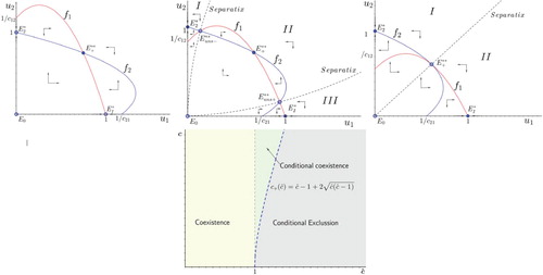
implies that (unconditional) global coexistence is not possible anymore, and either tri-stable conditional coexistence or conditional exclusion will happen, see Figure .
Figure 8. Competition outcomes of system (Equation4(4)
(4) ) in case of symmetric competition:
and
. Top left panel corresponds to global coexistence (
and any c>0). Central top panel corresponds to conditional coexistence (
and
). Top right panel corresponds conditional exclusion (
and
).
The classical model yields one species exclusion due to priority effects but, instead, a new dynamical scenario raises in the form of tri-stable conditional coexistence: depending on the initial number of individuals of each species either will coexist or one of them will go extinct. This result is straight against the classical thoughts [Citation13,Citation23,Citation35], although it makes perfect sense since, how can one distinguish intra from inter species competition in so similar species?
When competition is (perfectly) asymmetric, meaning that and that
, the classical model does not allow species coexistence, since mild competition (
for
) is not possible. However, the model presented herein allows bi-stable species coexistence in favour of the lower competitor if the upper competitor expends large enough time taking resources (see Proposition 4.3). Again, this result is at odds with classical results [Citation13,Citation23,Citation35] and illustrates the importance of looking carefully at how interactions take place.
Finally, we examine via numerical results the competition outcomes for the complete system (Equation4(4)
(4) ), that are not qualitatively different from the dynamical scenarios already shown. The source code used can be found in [Citation9].
We have found that for i = 1, 2 yield the existence of bi-stable conditional coexistence regions in favour of each species (see the dark red and dark blue regions in Figure ). The curves (that are not straight lines) delimiting such a regions are the counterparts of the curve
defined by (Equation10
(10)
(10) ), that we denote by
, for
. Note that while
is confined in the strap
, the curves
meet on
defining the so-called tri-stable conditional coexistence subregion. The classical model (Equation1
(1)
(1) ) predicts conditional exclusion due to priority effects in this region. Instead, model (Equation4
(4)
(4) ) allows species to coexist, again, provided that competitive abilities, initial values and competing time are well balanced, see Figure .
Figure 9. Competition outcomes of system (Equation4(4)
(4) ) as function of the competitive strengths
,
for a fixed value of
and increasing values of
. The code colour is the same as in Figure except the dark blue region that represents bi-stable conditional coexistence region in favour of species 1, dark-red region stands for bi-stable conditional coexistence region in favour of species 2 and the dark-grey region refers for the tri-stable conditional coexistence region. The figure is based on numerical calculations (the code is available in [Citation9]) and has been edited to improve it. Parameter values are
,
and, from left to right
.
![Figure 9. Competition outcomes of system (Equation4(4) u1′=r1u1−u12−c12u1u21+c1u1u2′=r2u2−u22−c21u2u11+c2u2(4) ) as function of the competitive strengths c12, c21 for a fixed value of c1 and increasing values of c2. The code colour is the same as in Figure 1 except the dark blue region that represents bi-stable conditional coexistence region in favour of species 1, dark-red region stands for bi-stable conditional coexistence region in favour of species 2 and the dark-grey region refers for the tri-stable conditional coexistence region. The figure is based on numerical calculations (the code is available in [Citation9]) and has been edited to improve it. Parameter values are 0<c12,c21<2, c1=1.9 and, from left to right c2=0,1.15,1.65,1.9,6,100,000.](/cms/asset/c9daaa9f-262e-40be-b698-004693ec2b61/tjbd_a_1742392_f0009_oc.jpg)
In words, in the strong competition scenario the mechanism(s) under the Holling type II competitive response play no role if only one of the species displays it, but facilitates coexistence when both species display it.
Note that the tri-stability region leans towards the axis if
and conversely. Indeed, consider a fixed value of
and lets see the effect of increasing
(see Figure ). As previously mentioned, a bi-stable coexistence region in favour of species 2 appears as
becomes larger than 0. Besides, the bi-stable coexistence region in favour of species 1 is reduced as
increases (see the panels in Figure ). Finally, numerical experiments suggest that the bi-stable coexistence region in favour of species 1 converges to a vertical strip as
(see bottom left panel in Figure ).
Interestingly, both bi- and tri-stable conditional coexistence have been also found in the context of competition models on patchy environments with individual dispersal [Citation25] or eco-epidemic competition models [Citation8].
Disclosure statement
No potential conflict of interest was reported by the authors.
ORCID
Hamlet Castillo-Alvino http://orcid.org/0000-0003-0335-1503
Marcos Marvá http://orcid.org/0000-0003-4703-8615
Additional information
Funding
References
- V. Ajraldi, M. Pittavino, and E. Venturino, Modeling herd behavior in population systems, Nonlinear Real-Anal. 12(4) (2011), pp. 2319–2338. doi: 10.1016/j.nonrwa.2011.02.002
- P. Amarasekare, Interference competition and species coexistence, P. Roy. Soc. B-Biol. Sci. 269(1509) (2002), pp. 2541–2550. doi: 10.1098/rspb.2002.2181
- P. Amarasekare, Competitive coexistence in spatially structured environments: A synthesis, Ecol. Lett.6 (2003), pp. 1109–1122. doi: 10.1046/j.1461-0248.2003.00530.x
- D.K. Arrowsmith, C.M. Place, Dynamical System: Differential Equations, Maps and Chaotic Behavior. 1st ed.Chapman Hall/CRC Mathematics Series, London, 1992.
- F.J. Ayala, M.E. Gilpin, and J.G. Ehrenfeld, Competition between species: Theoretical models and experimental tests, Theor. Popul. Biol. 4(3) (1973), pp. 331–356. doi: 10.1016/0040-5809(73)90014-2
- K.E. Barton, Natan J. Sanders, and D.M. Gordon, The effects of proximity and colony age on interspecific interference competition between the desert ants pogonomyrmex barbatus and aphaenogaster cockerelli, Amer. Midl. Naturalist. 180(1) (2009), pp. 376–382.
- J.R. Beddington, Mutual interference between parasites or predators and its effect on searching efficiency, J. Anim. Ecol. 44 (1975), pp. 331–340. doi: 10.2307/3866
- R. Bravo de la Parra, M. Marvá, E. Sánchezet al., Discrete models of disease and competition. Discrete Dyn. Nat. Soc. (2017), article id 5310837.
- H. Castillo-Alvino, (2019). Available at https://github.com/hcastilloa/code.
- P. Chesson, Mechamisms of maintenance of species diversity, Annu. Rev. Ecol. Syst. 31(3) (2000), pp. 43–66.
- P.H. Crowley and E.K. Martin, Functional responses and interference within and between year classes of a dragonfly population, J. North Am. Benthol. Soc. 8(3) (1989), pp. 211–221. doi: 10.2307/1467324
- D.L. De Angelis, R.A. Goldstein, and R.V. O'Neill, A model for trophic interaction, Ecology 56 (1975), pp. 881–892. doi: 10.2307/1936298
- G.F. Gause, The Struggle for Existence. Dover Books on Biology, Hafner, Baltimore, New York, 1934.
- W.M. Getz, Population dynamics: a per capita resource approach, J. Theor. Biol. 108 (1984), pp. 623–643. doi: 10.1016/S0022-5193(84)80082-X
- G. Hardin, The competitive exclusion principle, Science 131(3409) (1960), pp. 1292–1297. doi: 10.1126/science.131.3409.1292
- J. Hatcher and M.A.M. Dunn, Parasites in Ecological Communities From Interactions to Ecosystems, Cambridge University Press, Cambridge, 2011.
- C.S. Holling, Some characteristics of simple types of predation and parasitism, Can. Entomol. 91(7) (1959), p. 385. doi: 10.4039/Ent91385-7
- C.S. Holling, The component of predation as revealed by a study of small-mammal predation of the European pine sawfly, Can. Entomol. 91(5) (1959), pp. 293–320. doi: 10.4039/Ent91293-5
- H. Jiang and T.D. Rogers, The discrete dynamics of symmetrical competition on the plane, J. Math. Biol. 25(6) (1987), pp. 573–596. doi: 10.1007/BF00275495
- J.H. Lawton and M.P. Hassell, Asymmetrical competition in insects, Nature 289 (1981), pp. 793–795. doi: 10.1038/289793a0
- R. Levins, Evolution in Changing Environments, Princeton University Press, Princeton, 1968.
- S.A. Levin, Community equilibria and stability, and an extension of the competitive exclusion principle, Amer. Natur. 104(939) (1970), pp. 413–423. doi: 10.1086/282676
- A.J. Lotka, Elements of Physical Biology, Williams and Wilkins, Baltimore, 1925.
- R.H. MacArthur, Population ecology of some warblers of northeastern coniferous forests, Ecology 39 (1958), pp. 599–619. doi: 10.2307/1931600
- M. Marvá and R. Bravo de la Parra, Coexistence and superior competitor exclusion in the Leslie-Gower competition model with fast dispersal, Ecol. Model. 306 (2015), pp. 247–256. doi: 10.1016/j.ecolmodel.2014.10.039
- M. Marvá, A. Moussaoui, R. Bravo de la Parra, and P. Auger, A density dependent model describing age structured population dynamics using hawk-dove tactics, J. Differ. Equ. Appl. 19(6) (2013), pp. 1022–1034. doi: 10.1080/10236198.2012.707195
- D. Melchionda, E. Pastacaldi, and C. Perri, Social behavior-induced multistability in minimal competitive ecosystems, J. Theor. Biol. 439 (2018), pp. 24–38. doi: 10.1016/j.jtbi.2017.11.016
- A. Moussaoui, P. Auger, and B. Roche, Effect of Hawk-Dove game on the dynamics of two competing species, Acta Biotheor. 62(3) (2014), pp. 385–404. doi: 10.1007/s10441-014-9224-x
- D. Nguyen Ngoc, R. Bravo de la Parra, M.A. Zavala, and P. Auger, Competition and species coexistence in a metapopulation model: Can fast asymmetric migration reverse the outcome of competition in a homogeneous environment, J. Theo. Biol. 266 (2010), pp. 256–263. doi: 10.1016/j.jtbi.2010.06.020
- L. Nunney, Density compensation, isocline shape and single-level competition models, J. Theor. Biol.86 (1980), pp. 323–349. doi: 10.1016/0022-5193(80)90010-7
- T.W. Schoener, Effects of density-restricted food encounter some single-level competition models, Theor. Popul. Biol. 13 (1997), pp. 365–381. doi: 10.1016/0040-5809(78)90052-7
- G.T. Skalski and J.F. Gilliam, Functional responses with predator interference: Viable alternatives to the Holling Type II model, Ecology 82(11) (2001), pp. 3083–3092. doi: 10.1890/0012-9658(2001)082[3083:FRWPIV]2.0.CO;2
- M. Ritchie, Competition and coexistence of mobile animals, in Competition and Coexistence, U. Sommer and B. Worm, eds., Springer-Verlag, Berlin, 2002, pp. 109–131.
- S.B. Teleky, Multiple interactions: an empirically suggested model, Theor. Popul. Biol. 22 (1982), pp. 28–42. doi: 10.1016/0040-5809(82)90034-X
- V. Volterra, Variazioni e fluttuazioni del numero d'individui in specie animali conviventi, Mem. R. Accad. Naz. dei Lincei 2 (1926), pp. 31–113.
- J.B. Wilson, Mechanisms of species coexistence: twelve explanations for Hutchinson's “paradox of the plankton”: Evidence from New Zealand plant communities, N. Z. J. Ecol. 13 (1990), pp. 17–42.
- S.J. Wright, Plant diversity in tropical forests: a review of mechanisms of species coexistence, Oecologia130 (2002), pp. 1–14. doi: 10.1007/s004420100809
- Z. Zhang, Mututalism or cooperation among competitors promotes coexistence and competitive ability, Ecol. Model. 164 (2003), pp. 271–282. doi: 10.1016/S0304-3800(03)00069-3
- J. Zu, W. Wang, Y. Takeuchi, B. Zu, and K. Wang, On evolution under symmetric and asymmetric competitions, J. Theo. Biol. 254 (2008), pp. 239–251. doi: 10.1016/j.jtbi.2008.06.001