Age structured discrete-time disease models with demographic population cycles

Abstract

We use juvenile-adult discrete-time infectious disease models with intrinsically generated demographic population cycles to study the effects of age structure on the persistence or extinction of disease and the basic reproduction number, ${\mathcal{R}}_0$. Our juvenile-adult Susceptible-Infectious-Recovered (SIR) and Infectious-Salmon Anemia-Virus (ISA$v)$ models share a common disease-free system that exhibits equilibrium dynamics for the Beverton-Holt recruitment function. However, when the recruitment function is the Ricker model, a juvenile-adult disease-free system exhibits a range of dynamic behaviours from stable equilibria to deterministic period k population cycles to Neimark-Sacker bifurcations and deterministic chaos. For these two models, we use an extension of the next generation matrix approach for calculating ${\mathcal{R}}_0$ to account for populations with locally asymptotically stable period k cycles in the juvenile-adult disease-free system. When ${\mathcal{R}}_0<1$ and the juvenile-adult demographic system (in the absence of the disease) has a locally asymptotically stable period k population cycle, we prove that the juvenile-adult disease goes extinct whenever ${\mathcal{R}}_0<1$. Under the same period k juvenile-adult demographic assumption but with ${\mathcal{R}}_0>1$, we prove that the juvenile-adult disease-free period k population cycle is unstable and the disease persists. When ${\mathcal{R}}_0>1$, our simulations show that the juvenile-adult disease-free period k cycle dynamics drives the juvenile-adult SIR disease dynamics, but not the juvenile-adult ISAv disease dynamics.

Keywords:

• Adults
• Beverton-Holt model
• Juveniles
• population cycles
• Ricker model

1. Introduction

In many epidemiological models, the demographic (disease-free) state is a stable period k cycle $(k\ge 2)$, rather than a stable static non-cyclic equilibrium state $(k=1)$. When these demographic cycles are intrinsic to the model and are not generated from periodic perturbations, van den Driessche and Yakubu [35] in a recent paper, developed an extension of the next generation matrix (NGM) method for calculating the basic reproduction number, ${\mathcal{R}}_0$. In [35], a general autonomous deterministic discrete-time infectious disease model without age-structure was used to prove that ${\mathcal{R}}_0<1$ implies the local asymptotic stability of the period k disease-free population cycle and the disease goes extinct, whereas ${\mathcal{R}}_0>1$ implies the instability of the period k disease-free cycle and the disease invades the cyclic population.

The classic deterministic unstructured density-dependent Beverton-Holt [3,6,39] and Ricker [22,31,32,39] spawner-recruit discrete-time models are examples of simple single species models that have played fundamental roles in fisheries population dynamics. In the absence of environmental variability, the Beverton-Holt model exhibits stable equilibrium dynamics. However, unlike the Beverton-Holt model, the Ricker model is capable of generating a range of dynamic behaviours from stable equilibria to deterministic period k population cycles and deterministic chaos [24,26,31,32,39]. To understand the effects of introducing age-structure and disease into these models, especially regarding computing ${\mathcal{R}}_0$ when the demographic dynamics is cyclic, in this paper we focus on the effects of introducing juvenile-adult age structure into autonomous discrete-time epidemic models, where the density dependent recruitment function is either the Beverton-Holt or Ricker model. We use the NGM approach to two different juvenile-adult age structured discrete-time infectious disease models with the Beverton-Holt and Ricker demographic population dynamics, namely, a juvenile-adult age-structured Susceptible-Infectious-Recovered (SIR) model and a juvenile-adult age-structured infectious salmon anemia virus (ISAv) model [1,2,5,7,8,19,20,23,28–30,34–36].

Several authors have studied population models that allow for the interaction of density dependent demographic dynamics and age structure with or without explicit disease dynamics [4–6,9,10,15–18,24,37]. In this paper, our emphasis is on application of the NGM method to juvenile-adult discrete-time SIR and ISAv infectious disease models with intrinsically generated demographic population cycles. We compute ${\mathcal{R}}_0$ for these two models. When ${\mathcal{R}}_0>1$ and the juvenile-adult disease invades the populations, in agreement with the simulation results in [35] with unstructured models, our simulations show that the period of the juvenile-adult demographic disease-free state drives the period of the juvenile-adult SIR infectious population but not the period of the juvenile-adult ISAv infectious population.

In Section 2, we introduce the juvenile-adult SIR model with juvenile-adult demographic population cycles and compute ${\mathcal{R}}_0$. When the recruitment function is either the Beverton-Holt or Ricker model, in Section 3, we use simulations to explore the relationship between the period of the juvenile-adult demographic population and the period of the juvenile-adult SIR infectious population. The juvenile-adult ISAv model is introduced in Section 4, and the relationship between the juvenile-adult periodic demographic population dynamics and the period of the juvenile-adult ISAv infectious population is discussed in Section 5. We summarize our results in the Concluding Remarks section.

2. Juvenile-Adult discrete-time SIR epidemic model

To introduce a juvenile-adult age structured Susceptible-Infectious-Recovered (SIR) discrete-time disease epidemic model, we assume that at each time $t\in \{0,1,2,\dots \}$, each member of a population is either a susceptible juvenile $\left(S_t^J\right)$, susceptible adult $\left(S_t^A\right)$, infectious juvenile (infected with the disease, $I_t^J$), infectious adult (infected with the disease, $I_t^A$), recovered juvenile from the disease $\left(R_t^J\right)$ or recovered adult $\left(R_t^A\right)$ with life-long immunity, where the total juvenile and adult populations are respectively $N_t^J=S_t^J+I_t^J+R_t^J\mathrm{a}\mathrm{n}\mathrm{d}{N}_t^A=S_t^A+I_t^A+R_t^A.$ That is, at each time t, we let $S_t^{\mathrm{\Lambda }}$, $I_t^{\mathrm{\Lambda }}$, $R_t^{\mathrm{\Lambda }}$ and $N_t^{\mathrm{\Lambda }}$, respectively denote the population numbers of susceptible, infectious, recovered and total population of juveniles when $\mathrm{\Lambda }=J$ or adults when $\mathrm{\Lambda }=A$. The overall total population at time t is $N_t=N_t^J+N_t^A.$ From time t to time t + 1, we assume that a susceptible individual encounters either infectious juveniles or infectious adults. Thus, the probability of exposure of an individual to multiple infection pathways in the unit interval is low and so can be ignored. Consequently, at each time t, we assume per unit time interval that a fraction of susceptible juveniles, ${\theta }_J{S}_t^J$, that interact with infectious juveniles become infectious juveniles with probability ${\hat{\varphi }}_J\left(I_t^J\right)=(1-{\varphi }_J(I_t^J\left)\right)$ (remain susceptible juveniles with probability ${\varphi }_J\left(I_t^J\right)$) and the remaining fraction of susceptible juveniles, $(1-{\theta }_J)S_t^J$, that interact with infectious adults become infectious juveniles with probability ${\hat{\varphi }}_J\left(I_t^A\right)=(1-{\varphi }_J(I_t^A\left)\right)$ (remain susceptible juveniles with probability ${\varphi }_J\left(I_t^A\right)$). Similarly, per unit time interval a fraction of susceptible adults, ${\theta }_A{S}_t^A$, that interact with infectious juveniles become infectious adults with probability ${\hat{\varphi }}_A\left(I_t^J\right)=(1-{\varphi }_A(I_t^J\left)\right)$ (remain susceptible adults with probability ${\varphi }_A\left(I_t^J\right)$) and the remaining fraction of susceptible adults, $(1-{\theta }_A)S_t^A$, that interact with infectious adults become infectious adults with probability ${\hat{\varphi }}_A\left(I_t^A\right)=(1-{\varphi }_A(I_t^A\left)\right)$ (remain susceptible adults with probability ${\varphi }_A\left(I_t^A\right)$).

For each $\mathrm{\Lambda }\in \{A,J\}$, the ‘escape’ function ${\varphi }_{\mathrm{\Lambda }}:{\mathbb{R}}_{+}\to [0,1]$ is a nonlinear decreasing smooth concave up function with ${\varphi }_{\mathrm{\Lambda }}\left(0\right)=1$, and ${\mathbb{R}}_{+}=[0,\mathrm{\infty })$. That is, ${\varphi }_{\mathrm{\Lambda }}^{\mathrm{\prime }}\left(I^{\mathrm{\Lambda }}\right)<0$ and ${\varphi }_{\mathrm{\Lambda }}^{\mathrm{\prime }\mathrm{\prime }}\left(I^{\mathrm{\Lambda }}\right)>0$ for all $I^{\mathrm{\Lambda }}\ge 0$. For example, when infections are modelled as Poisson processes, then ${\varphi }_{\mathrm{\Lambda }}\left(I^{\mathrm{\Lambda }}\right)=\exp (-\text{β}{I}^{\mathrm{\Lambda }})$ with the transmission constant $\text{β}>0$. In all our examples, we will use the Poisson distribution to model infections in the juvenile and adult populations. However, other distributions that satisfy our assumptions on ${\varphi }_{\mathrm{\Lambda }}$ could be used to obtain similar results.

Furthermore, we assume that the fraction of infectious juveniles that recover from the infection is ${\gamma }_J\in (0,1)$, and the fraction that remains infectious is ${\hat{\gamma }}_J=(1-{\gamma }_J)$ per unit time interval. Similarly, we assume that the fraction of infectious adults that recover from the infection is ${\gamma }_A\in (0,1)$, and the fraction that remains infectious is ${\hat{\gamma }}_A=(1-{\gamma }_A)$ per unit time interval. We model a disease that is not fatal so we ignore death due to the disease. We assume that the fraction of juveniles (respectively, adults) that die from natural causes is $d_J\in (0,1)$ (respectively, $d_A\in (0,1)$), and the fraction that stay alive per unit interval is ${\hat{d}}_J=(1-d_J)$ (respectively, ${\hat{d}}_A=(1-d_A)$). In most fish populations, the fraction that die from natural causes is highest in early life; thus, we take $d_A\le d_J$. In our model, a susceptible individual is to be in the infectious class before recovering, and recovered individuals have life-long immunity. During each time interval, we assume that a constant fraction of juveniles, m $\in (0,1)$, mature to adulthood and the fraction, $\hat{m}=(1-m)$, remain in the juvenile class.

To include demographic dynamics, we let $g:{\mathbb{R}}_{+}\to {\mathbb{R}}_{+}$ denote the nonlinear differentiable recruitment (or birth) function of adults into the susceptible juvenile class per unit time interval, where $g\left(N_t^A\right)=N_t^{A}h\left(N_t^A\right).$ To prevent unbounded population growth, we assume that the per capita growth function, $h:{\mathbb{R}}_{+}\to \mathbb{(}0,\mathrm{\infty }),$ is a positive strictly decreasing smooth function and $\underset{N_t^A\to \mathrm{\infty }}{lim}h\left(N_t^A\right)=0.$ The Beverton-Holt model [3,6,39], $g\left(N_t^A\right)=\frac{r{N}_t^A}{1+b{N}_t^A}\mathrm{a}\mathrm{n}\mathrm{d}h\left(N_t^A\right)=\frac{r}{1+b{N}_t^A},$ and the Ricker model [22,31,32,39], $g\left(N_t^A\right)=r{N}_t^A\exp \left(-b{N}_t^A\right)\mathrm{a}\mathrm{n}\mathrm{d}h\left(N_t^A\right)=r\exp \left(-b{N}_t^A\right)$ are examples of simple spawner-recruitment and per-capita growth functions that have played fundamental roles in fishery science for many years. These models are widely considered as potential management tools. For the Beverton-Holt model, the positive parameters r and b characterize the density-dependent reproductive phase. That is, r is the density-independent per-capita growth rate when the population is very small, and $r/b$ is the maximum total number of offspring in the fish population [3,6]. For the Ricker model, r is the density-independent probability of survival from egg to age 1, and b is the coefficient of density-dependent mortality [22,31,32]. These models are examples of recruitment functions in this study.

Our assumptions and notation lead to the following discrete-time juvenile-adult SIR epidemic model. (1) $\left.\begin{array}{rl}{S}_{t+1}^J& =g\left(N_t^A\right)+{\hat{d}}_J\hat{m}{S}_t^J\left({\theta }_J{\varphi }_J\left(I_t^J\right)+\left(1-{\theta }_J\right){\varphi }_J\left(I_t^A\right)\right)\\ I_{t+1}^J& ={\hat{d}}_J\hat{m}{S}_t^J\left({\theta }_J{\hat{\varphi }}_J\left(I_t^J\right)+\left(1-{\theta }_J\right){\hat{\varphi }}_J\left(I_t^A\right)\right)+{\hat{d}}_J\hat{m}{\hat{\gamma }}_J{I}_t^J\\ R_{t+1}^J& ={\hat{d}}_J\hat{m}{\gamma }_J{I}_t^J+{\hat{d}}_J\hat{m}{R}_t^J\\ S_{t+1}^A& ={\hat{d}}_A\left(m{S}_t^J+S_t^A\right)\left({\theta }_A{\varphi }_A\left(I_t^J\right)+\left(1-{\theta }_A\right){\varphi }_A\left(I_t^A\right)\right)\\ I_{t+1}^A& ={\hat{d}}_A\left(m{S}_t^J+S_t^A\right)\left({\theta }_A{\hat{\varphi }}_A\left(I_t^J\right)+\left(1-{\theta }_A\right){\hat{\varphi }}_A\left(I_t^A\right)\right)+{\hat{d}}_A{\hat{\gamma }}_A\left(m{I}_t^J+I_t^A\right)\\ R_{t+1}^A& ={\hat{d}}_A{\gamma }_A\left(m{I}_t^J+I_t^A\right)+{\hat{d}}_A\left(m{R}_t^J+R_t^A\right)\end{array}\right\}$(1) where $t=0,1,2,\dots$.

We study Model (1(1) $\left.\begin{array}{rl}{S}_{t+1}^J& =g\left(N_t^A\right)+{\hat{d}}_J\hat{m}{S}_t^J\left({\theta }_J{\varphi }_J\left(I_t^J\right)+\left(1-{\theta }_J\right){\varphi }_J\left(I_t^A\right)\right)\\ I_{t+1}^J& ={\hat{d}}_J\hat{m}{S}_t^J\left({\theta }_J{\hat{\varphi }}_J\left(I_t^J\right)+\left(1-{\theta }_J\right){\hat{\varphi }}_J\left(I_t^A\right)\right)+{\hat{d}}_J\hat{m}{\hat{\gamma }}_J{I}_t^J\\ R_{t+1}^J& ={\hat{d}}_J\hat{m}{\gamma }_J{I}_t^J+{\hat{d}}_J\hat{m}{R}_t^J\\ S_{t+1}^A& ={\hat{d}}_A\left(m{S}_t^J+S_t^A\right)\left({\theta }_A{\varphi }_A\left(I_t^J\right)+\left(1-{\theta }_A\right){\varphi }_A\left(I_t^A\right)\right)\\ I_{t+1}^A& ={\hat{d}}_A\left(m{S}_t^J+S_t^A\right)\left({\theta }_A{\hat{\varphi }}_A\left(I_t^J\right)+\left(1-{\theta }_A\right){\hat{\varphi }}_A\left(I_t^A\right)\right)+{\hat{d}}_A{\hat{\gamma }}_A\left(m{I}_t^J+I_t^A\right)\\ R_{t+1}^A& ={\hat{d}}_A{\gamma }_A\left(m{I}_t^J+I_t^A\right)+{\hat{d}}_A\left(m{R}_t^J+R_t^A\right)\end{array}\right\}$(1) ) with initial conditions $\left(S_0^J,I_0^J,R_0^J,S_0^A,I_0^A,R_0^A\right)\in {\mathbb{R}}_{+}^6.$ In Model (1(1) $\left.\begin{array}{rl}{S}_{t+1}^J& =g\left(N_t^A\right)+{\hat{d}}_J\hat{m}{S}_t^J\left({\theta }_J{\varphi }_J\left(I_t^J\right)+\left(1-{\theta }_J\right){\varphi }_J\left(I_t^A\right)\right)\\ I_{t+1}^J& ={\hat{d}}_J\hat{m}{S}_t^J\left({\theta }_J{\hat{\varphi }}_J\left(I_t^J\right)+\left(1-{\theta }_J\right){\hat{\varphi }}_J\left(I_t^A\right)\right)+{\hat{d}}_J\hat{m}{\hat{\gamma }}_J{I}_t^J\\ R_{t+1}^J& ={\hat{d}}_J\hat{m}{\gamma }_J{I}_t^J+{\hat{d}}_J\hat{m}{R}_t^J\\ S_{t+1}^A& ={\hat{d}}_A\left(m{S}_t^J+S_t^A\right)\left({\theta }_A{\varphi }_A\left(I_t^J\right)+\left(1-{\theta }_A\right){\varphi }_A\left(I_t^A\right)\right)\\ I_{t+1}^A& ={\hat{d}}_A\left(m{S}_t^J+S_t^A\right)\left({\theta }_A{\hat{\varphi }}_A\left(I_t^J\right)+\left(1-{\theta }_A\right){\hat{\varphi }}_A\left(I_t^A\right)\right)+{\hat{d}}_A{\hat{\gamma }}_A\left(m{I}_t^J+I_t^A\right)\\ R_{t+1}^A& ={\hat{d}}_A{\gamma }_A\left(m{I}_t^J+I_t^A\right)+{\hat{d}}_A\left(m{R}_t^J+R_t^A\right)\end{array}\right\}$(1) ), we assume that events happen in the following order: disease transmission and recovery then juvenile maturity to adulthood; survival (natural death); and reproduction or recruitment. However, in real biological systems, these three events may happen in different orders. When there is no age-structure and the model consists of only adults (without juveniles), and the disease is short lived compared to the population lifetime, then $g\left(N_t^A\right)=d_A={\theta }_A=0,$ and Model (1(1) $\left.\begin{array}{rl}{S}_{t+1}^J& =g\left(N_t^A\right)+{\hat{d}}_J\hat{m}{S}_t^J\left({\theta }_J{\varphi }_J\left(I_t^J\right)+\left(1-{\theta }_J\right){\varphi }_J\left(I_t^A\right)\right)\\ I_{t+1}^J& ={\hat{d}}_J\hat{m}{S}_t^J\left({\theta }_J{\hat{\varphi }}_J\left(I_t^J\right)+\left(1-{\theta }_J\right){\hat{\varphi }}_J\left(I_t^A\right)\right)+{\hat{d}}_J\hat{m}{\hat{\gamma }}_J{I}_t^J\\ R_{t+1}^J& ={\hat{d}}_J\hat{m}{\gamma }_J{I}_t^J+{\hat{d}}_J\hat{m}{R}_t^J\\ S_{t+1}^A& ={\hat{d}}_A\left(m{S}_t^J+S_t^A\right)\left({\theta }_A{\varphi }_A\left(I_t^J\right)+\left(1-{\theta }_A\right){\varphi }_A\left(I_t^A\right)\right)\\ I_{t+1}^A& ={\hat{d}}_A\left(m{S}_t^J+S_t^A\right)\left({\theta }_A{\hat{\varphi }}_A\left(I_t^J\right)+\left(1-{\theta }_A\right){\hat{\varphi }}_A\left(I_t^A\right)\right)+{\hat{d}}_A{\hat{\gamma }}_A\left(m{I}_t^J+I_t^A\right)\\ R_{t+1}^A& ={\hat{d}}_A{\gamma }_A\left(m{I}_t^J+I_t^A\right)+{\hat{d}}_A\left(m{R}_t^J+R_t^A\right)\end{array}\right\}$(1) ) reduces to the well-studied discrete-time SIR model with no demographic effects [1,7].

Firstly, we prove that Model (1(1) $\left.\begin{array}{rl}{S}_{t+1}^J& =g\left(N_t^A\right)+{\hat{d}}_J\hat{m}{S}_t^J\left({\theta }_J{\varphi }_J\left(I_t^J\right)+\left(1-{\theta }_J\right){\varphi }_J\left(I_t^A\right)\right)\\ I_{t+1}^J& ={\hat{d}}_J\hat{m}{S}_t^J\left({\theta }_J{\hat{\varphi }}_J\left(I_t^J\right)+\left(1-{\theta }_J\right){\hat{\varphi }}_J\left(I_t^A\right)\right)+{\hat{d}}_J\hat{m}{\hat{\gamma }}_J{I}_t^J\\ R_{t+1}^J& ={\hat{d}}_J\hat{m}{\gamma }_J{I}_t^J+{\hat{d}}_J\hat{m}{R}_t^J\\ S_{t+1}^A& ={\hat{d}}_A\left(m{S}_t^J+S_t^A\right)\left({\theta }_A{\varphi }_A\left(I_t^J\right)+\left(1-{\theta }_A\right){\varphi }_A\left(I_t^A\right)\right)\\ I_{t+1}^A& ={\hat{d}}_A\left(m{S}_t^J+S_t^A\right)\left({\theta }_A{\hat{\varphi }}_A\left(I_t^J\right)+\left(1-{\theta }_A\right){\hat{\varphi }}_A\left(I_t^A\right)\right)+{\hat{d}}_A{\hat{\gamma }}_A\left(m{I}_t^J+I_t^A\right)\\ R_{t+1}^A& ={\hat{d}}_A{\gamma }_A\left(m{I}_t^J+I_t^A\right)+{\hat{d}}_A\left(m{R}_t^J+R_t^A\right)\end{array}\right\}$(1) ) is well-posed.

Theorem 2.1

In Model (1(1) $\left.\begin{array}{rl}{S}_{t+1}^J& =g\left(N_t^A\right)+{\hat{d}}_J\hat{m}{S}_t^J\left({\theta }_J{\varphi }_J\left(I_t^J\right)+\left(1-{\theta }_J\right){\varphi }_J\left(I_t^A\right)\right)\\ I_{t+1}^J& ={\hat{d}}_J\hat{m}{S}_t^J\left({\theta }_J{\hat{\varphi }}_J\left(I_t^J\right)+\left(1-{\theta }_J\right){\hat{\varphi }}_J\left(I_t^A\right)\right)+{\hat{d}}_J\hat{m}{\hat{\gamma }}_J{I}_t^J\\ R_{t+1}^J& ={\hat{d}}_J\hat{m}{\gamma }_J{I}_t^J+{\hat{d}}_J\hat{m}{R}_t^J\\ S_{t+1}^A& ={\hat{d}}_A\left(m{S}_t^J+S_t^A\right)\left({\theta }_A{\varphi }_A\left(I_t^J\right)+\left(1-{\theta }_A\right){\varphi }_A\left(I_t^A\right)\right)\\ I_{t+1}^A& ={\hat{d}}_A\left(m{S}_t^J+S_t^A\right)\left({\theta }_A{\hat{\varphi }}_A\left(I_t^J\right)+\left(1-{\theta }_A\right){\hat{\varphi }}_A\left(I_t^A\right)\right)+{\hat{d}}_A{\hat{\gamma }}_A\left(m{I}_t^J+I_t^A\right)\\ R_{t+1}^A& ={\hat{d}}_A{\gamma }_A\left(m{I}_t^J+I_t^A\right)+{\hat{d}}_A\left(m{R}_t^J+R_t^A\right)\end{array}\right\}$(1) ) with $\left(S_0^J,I_0^J,R_0^J,S_0^A,I_0^A,R_0^A\right)\in {\mathbb{R}}_{+}^6,$ for each time $t\in \{1,2,\dots \},$ $\left(S_t^J,I_t^J,R_t^J,S_t^A,I_t^A,R_t^A\right)\in {\mathbb{R}}_{+}^6,$ and there is no unbounded population growth.

Proof.

Since $(S_0^J,I_0^J,R_0^J,S_0^A,I_0^A,R_0^A)\in {\mathbb{R}}_{+}^6$, each equation of Model (1(1) $\left.\begin{array}{rl}{S}_{t+1}^J& =g\left(N_t^A\right)+{\hat{d}}_J\hat{m}{S}_t^J\left({\theta }_J{\varphi }_J\left(I_t^J\right)+\left(1-{\theta }_J\right){\varphi }_J\left(I_t^A\right)\right)\\ I_{t+1}^J& ={\hat{d}}_J\hat{m}{S}_t^J\left({\theta }_J{\hat{\varphi }}_J\left(I_t^J\right)+\left(1-{\theta }_J\right){\hat{\varphi }}_J\left(I_t^A\right)\right)+{\hat{d}}_J\hat{m}{\hat{\gamma }}_J{I}_t^J\\ R_{t+1}^J& ={\hat{d}}_J\hat{m}{\gamma }_J{I}_t^J+{\hat{d}}_J\hat{m}{R}_t^J\\ S_{t+1}^A& ={\hat{d}}_A\left(m{S}_t^J+S_t^A\right)\left({\theta }_A{\varphi }_A\left(I_t^J\right)+\left(1-{\theta }_A\right){\varphi }_A\left(I_t^A\right)\right)\\ I_{t+1}^A& ={\hat{d}}_A\left(m{S}_t^J+S_t^A\right)\left({\theta }_A{\hat{\varphi }}_A\left(I_t^J\right)+\left(1-{\theta }_A\right){\hat{\varphi }}_A\left(I_t^A\right)\right)+{\hat{d}}_A{\hat{\gamma }}_A\left(m{I}_t^J+I_t^A\right)\\ R_{t+1}^A& ={\hat{d}}_A{\gamma }_A\left(m{I}_t^J+I_t^A\right)+{\hat{d}}_A\left(m{R}_t^J+R_t^A\right)\end{array}\right\}$(1) ) is a sum of nonnegative terms. Hence, $(S_t^J,I_t^J,R_t^J,S_t^A,I_t^A,R_t^A)\in {\mathbb{R}}_{+}^6$ for all $t\ge 0$. Summing the first three juvenile (respectively, last three adult) equations of Model (1(1) $\left.\begin{array}{rl}{S}_{t+1}^J& =g\left(N_t^A\right)+{\hat{d}}_J\hat{m}{S}_t^J\left({\theta }_J{\varphi }_J\left(I_t^J\right)+\left(1-{\theta }_J\right){\varphi }_J\left(I_t^A\right)\right)\\ I_{t+1}^J& ={\hat{d}}_J\hat{m}{S}_t^J\left({\theta }_J{\hat{\varphi }}_J\left(I_t^J\right)+\left(1-{\theta }_J\right){\hat{\varphi }}_J\left(I_t^A\right)\right)+{\hat{d}}_J\hat{m}{\hat{\gamma }}_J{I}_t^J\\ R_{t+1}^J& ={\hat{d}}_J\hat{m}{\gamma }_J{I}_t^J+{\hat{d}}_J\hat{m}{R}_t^J\\ S_{t+1}^A& ={\hat{d}}_A\left(m{S}_t^J+S_t^A\right)\left({\theta }_A{\varphi }_A\left(I_t^J\right)+\left(1-{\theta }_A\right){\varphi }_A\left(I_t^A\right)\right)\\ I_{t+1}^A& ={\hat{d}}_A\left(m{S}_t^J+S_t^A\right)\left({\theta }_A{\hat{\varphi }}_A\left(I_t^J\right)+\left(1-{\theta }_A\right){\hat{\varphi }}_A\left(I_t^A\right)\right)+{\hat{d}}_A{\hat{\gamma }}_A\left(m{I}_t^J+I_t^A\right)\\ R_{t+1}^A& ={\hat{d}}_A{\gamma }_A\left(m{I}_t^J+I_t^A\right)+{\hat{d}}_A\left(m{R}_t^J+R_t^A\right)\end{array}\right\}$(1) ), at each time $t\in \{0,1,2,\dots \}$, the juvenile (respectively, adult) total populations are governed by $N_{t+1}^J=g\left(N_t^A\right)+{\hat{d}}_J\hat{m}{N}_t^J$ and $N_{t+1}^A={\hat{d}}_A{N}_t^A+{\hat{d}}_{A}m{N}_t^J.$ Hence, the total population, $N_t=N_t^J+N_t^A\ge 0$, is governed by $N_{t+1}\le g\left(N_t^A\right)+{\hat{d}}_A{N}_t^J+{\hat{d}}_A{N}_t^A\le g\left(N_t^A\right)+{\hat{d}}_A{N}_t,$ where $d_A\le d_J$. Since $g\left(N_t^A\right)=N_t^{A}h\left(N_t^A\right)\ge 0$ is a smooth function and $\underset{N_t^A\to \mathrm{\infty }}{lim}h\left(N_t^A\right)=0,$ there exists K>0 and a sufficiently small $\epsilon \in (0,1)$ such that $h\left(N_t^A\right)<\epsilon$ for all $t\ge K$. Thus, $N_{t+1}\le \left(\epsilon +{\hat{d}}_A\right)N_t<N_t$ for all $t\ge K$, where $N_0>0$. Consequently, $\underset{t\to \mathrm{\infty }}{lim}{N}_t<\mathrm{\infty }$, the set of iterates of all non-negative initial population numbers are bounded and there is no unbounded population growth in Model (1(1) $\left.\begin{array}{rl}{S}_{t+1}^J& =g\left(N_t^A\right)+{\hat{d}}_J\hat{m}{S}_t^J\left({\theta }_J{\varphi }_J\left(I_t^J\right)+\left(1-{\theta }_J\right){\varphi }_J\left(I_t^A\right)\right)\\ I_{t+1}^J& ={\hat{d}}_J\hat{m}{S}_t^J\left({\theta }_J{\hat{\varphi }}_J\left(I_t^J\right)+\left(1-{\theta }_J\right){\hat{\varphi }}_J\left(I_t^A\right)\right)+{\hat{d}}_J\hat{m}{\hat{\gamma }}_J{I}_t^J\\ R_{t+1}^J& ={\hat{d}}_J\hat{m}{\gamma }_J{I}_t^J+{\hat{d}}_J\hat{m}{R}_t^J\\ S_{t+1}^A& ={\hat{d}}_A\left(m{S}_t^J+S_t^A\right)\left({\theta }_A{\varphi }_A\left(I_t^J\right)+\left(1-{\theta }_A\right){\varphi }_A\left(I_t^A\right)\right)\\ I_{t+1}^A& ={\hat{d}}_A\left(m{S}_t^J+S_t^A\right)\left({\theta }_A{\hat{\varphi }}_A\left(I_t^J\right)+\left(1-{\theta }_A\right){\hat{\varphi }}_A\left(I_t^A\right)\right)+{\hat{d}}_A{\hat{\gamma }}_A\left(m{I}_t^J+I_t^A\right)\\ R_{t+1}^A& ={\hat{d}}_A{\gamma }_A\left(m{I}_t^J+I_t^A\right)+{\hat{d}}_A\left(m{R}_t^J+R_t^A\right)\end{array}\right\}$(1) ).

At each time $t\in \{0,1,2,\dots \}$, when $I_t^J=I_t^A=R_t^J=R_t^A=0,$ Model (1(1) $\left.\begin{array}{rl}{S}_{t+1}^J& =g\left(N_t^A\right)+{\hat{d}}_J\hat{m}{S}_t^J\left({\theta }_J{\varphi }_J\left(I_t^J\right)+\left(1-{\theta }_J\right){\varphi }_J\left(I_t^A\right)\right)\\ I_{t+1}^J& ={\hat{d}}_J\hat{m}{S}_t^J\left({\theta }_J{\hat{\varphi }}_J\left(I_t^J\right)+\left(1-{\theta }_J\right){\hat{\varphi }}_J\left(I_t^A\right)\right)+{\hat{d}}_J\hat{m}{\hat{\gamma }}_J{I}_t^J\\ R_{t+1}^J& ={\hat{d}}_J\hat{m}{\gamma }_J{I}_t^J+{\hat{d}}_J\hat{m}{R}_t^J\\ S_{t+1}^A& ={\hat{d}}_A\left(m{S}_t^J+S_t^A\right)\left({\theta }_A{\varphi }_A\left(I_t^J\right)+\left(1-{\theta }_A\right){\varphi }_A\left(I_t^A\right)\right)\\ I_{t+1}^A& ={\hat{d}}_A\left(m{S}_t^J+S_t^A\right)\left({\theta }_A{\hat{\varphi }}_A\left(I_t^J\right)+\left(1-{\theta }_A\right){\hat{\varphi }}_A\left(I_t^A\right)\right)+{\hat{d}}_A{\hat{\gamma }}_A\left(m{I}_t^J+I_t^A\right)\\ R_{t+1}^A& ={\hat{d}}_A{\gamma }_A\left(m{I}_t^J+I_t^A\right)+{\hat{d}}_A\left(m{R}_t^J+R_t^A\right)\end{array}\right\}$(1) ) reduces to the following disease-free system of two equations. (2) $\left.\begin{array}{rl}{S}_{t+1}^J& =g\left(S_t^A\right)+\left(1-d_J\right)\left(1-m\right)S_t^J\\ S_{t+1}^A& =\left(1-d_A\right)\left(m{S}_t^J+S_t^A\right)\end{array}\right\}$(2) Unlike the unstructured SIR model in [35], the disease-free system of the juvenile-adult Model (1(1) $\left.\begin{array}{rl}{S}_{t+1}^J& =g\left(N_t^A\right)+{\hat{d}}_J\hat{m}{S}_t^J\left({\theta }_J{\varphi }_J\left(I_t^J\right)+\left(1-{\theta }_J\right){\varphi }_J\left(I_t^A\right)\right)\\ I_{t+1}^J& ={\hat{d}}_J\hat{m}{S}_t^J\left({\theta }_J{\hat{\varphi }}_J\left(I_t^J\right)+\left(1-{\theta }_J\right){\hat{\varphi }}_J\left(I_t^A\right)\right)+{\hat{d}}_J\hat{m}{\hat{\gamma }}_J{I}_t^J\\ R_{t+1}^J& ={\hat{d}}_J\hat{m}{\gamma }_J{I}_t^J+{\hat{d}}_J\hat{m}{R}_t^J\\ S_{t+1}^A& ={\hat{d}}_A\left(m{S}_t^J+S_t^A\right)\left({\theta }_A{\varphi }_A\left(I_t^J\right)+\left(1-{\theta }_A\right){\varphi }_A\left(I_t^A\right)\right)\\ I_{t+1}^A& ={\hat{d}}_A\left(m{S}_t^J+S_t^A\right)\left({\theta }_A{\hat{\varphi }}_A\left(I_t^J\right)+\left(1-{\theta }_A\right){\hat{\varphi }}_A\left(I_t^A\right)\right)+{\hat{d}}_A{\hat{\gamma }}_A\left(m{I}_t^J+I_t^A\right)\\ R_{t+1}^A& ={\hat{d}}_A{\gamma }_A\left(m{I}_t^J+I_t^A\right)+{\hat{d}}_A\left(m{R}_t^J+R_t^A\right)\end{array}\right\}$(1) ) is a system of two equations. In the next section, we analyze Model (2(2) $\left.\begin{array}{rl}{S}_{t+1}^J& =g\left(S_t^A\right)+\left(1-d_J\right)\left(1-m\right)S_t^J\\ S_{t+1}^A& =\left(1-d_A\right)\left(m{S}_t^J+S_t^A\right)\end{array}\right\}$(2) ).

2.1. Juvenile-adult disease-free demographic system

The origin, $\left(S_{-}^J,S_{-}^A\right)=\left(0,0\right),$ is the trivial equilibrium point of Model (2(2) $\left.\begin{array}{rl}{S}_{t+1}^J& =g\left(S_t^A\right)+\left(1-d_J\right)\left(1-m\right)S_t^J\\ S_{t+1}^A& =\left(1-d_A\right)\left(m{S}_t^J+S_t^A\right)\end{array}\right\}$(2) ). To determine the stability of the origin, we proceed as in the NGM method approach to obtain the juvenile-adult demographic threshold parameter for Model (2(2) $\left.\begin{array}{rl}{S}_{t+1}^J& =g\left(S_t^A\right)+\left(1-d_J\right)\left(1-m\right)S_t^J\\ S_{t+1}^A& =\left(1-d_A\right)\left(m{S}_t^J+S_t^A\right)\end{array}\right\}$(2) ), ${\mathcal{R}}_d=\rho \left(F{\left(I_d-T\right)}^{-1}\right)=\frac{m\left(1-d_A\right)h\left(0\right)}{d_A\left(1-\left(1-d_J\right)\left(1-m\right)\right)},$ where $\rho \left(F\right(I_d-T{)}^{-1})$ is the spectral radius of $F(I_d-T{)}^{-1}$, $F=\left[\begin{array}{cc}0& h\left(0\right)\\ 0& 0\end{array}\right]\mathrm{a}\mathrm{n}\mathrm{d}T=\left[\begin{array}{cc}\left(1-d_J\right)\left(1-m\right)& 0\\ \left(1-d_A\right)m& \left(1-d_A\right)\end{array}\right],$ where $I_d$ is the identity matrix. If $S^A$ is a positive fixed point of Model (2(2) $\left.\begin{array}{rl}{S}_{t+1}^J& =g\left(S_t^A\right)+\left(1-d_J\right)\left(1-m\right)S_t^J\\ S_{t+1}^A& =\left(1-d_A\right)\left(m{S}_t^J+S_t^A\right)\end{array}\right\}$(2) ), then (3) $h\left(S^A\right)=\frac{h\left(0\right)}{{\mathcal{R}}_d}.$(3) Recall that h is strictly decreasing, positive and smooth with $\underset{S^A\to \mathrm{\infty }}{lim}h\left(S^A\right)=0$. Thus, $h\left(0\right)>h\left(S^A\right)$ for any $S^A>0$. Consequently, for any $S^A>0$ and ${\mathcal{R}}_d\le 1$, $\frac{h\left(0\right)}{{\mathcal{R}}_d}\ge h\left(0\right)>h\left(S^A\right).$ That is, whenever ${\mathcal{R}}_d\le 1$, there exists no $S^A>0$ that satisfies (3(3) $h\left(S^A\right)=\frac{h\left(0\right)}{{\mathcal{R}}_d}.$(3) ), and Model (2(2) $\left.\begin{array}{rl}{S}_{t+1}^J& =g\left(S_t^A\right)+\left(1-d_J\right)\left(1-m\right)S_t^J\\ S_{t+1}^A& =\left(1-d_A\right)\left(m{S}_t^J+S_t^A\right)\end{array}\right\}$(2) ) has only the trivial equilibrium point. However, $\frac{h\left(0\right)}{{\mathcal{R}}_d}<h\left(0\right)\mathrm{w}\mathrm{h}\mathrm{e}\mathrm{n}\mathrm{e}\mathrm{v}\mathrm{e}\mathrm{r}{\mathcal{R}}_d>1.$ The monotonicity condition on h and the fact that $\underset{S^A\to \mathrm{\infty }}{lim}h\left(S^A\right)=0$ imply that there exists a unique $S_{+}^A>0$ satisfying (3(3) $h\left(S^A\right)=\frac{h\left(0\right)}{{\mathcal{R}}_d}.$(3) ) whenever ${\mathcal{R}}_d>1$. Hence, when ${\mathcal{R}}_d>1$, Model (2(2) $\left.\begin{array}{rl}{S}_{t+1}^J& =g\left(S_t^A\right)+\left(1-d_J\right)\left(1-m\right)S_t^J\\ S_{t+1}^A& =\left(1-d_A\right)\left(m{S}_t^J+S_t^A\right)\end{array}\right\}$(2) ) has only exactly the two equilibrium points, $\left(S_{-}^J,S_{-}^A\right)=\left(0,0\right)\mathrm{a}\mathrm{n}\mathrm{d}\left(S_{+}^J,S_{+}^A\right)=\left(\frac{d_A{S}_{+}^A}{m\left(1-d_A\right)},S_{+}^A\right),$ where $S_{+}^A>0\mathrm{a}\mathrm{n}\mathrm{d}h\left(S_{+}^A\right)=\frac{h\left(0\right)}{{\mathcal{R}}_d}.$

Theorem 2.2

In Model (2(2) $\left.\begin{array}{rl}{S}_{t+1}^J& =g\left(S_t^A\right)+\left(1-d_J\right)\left(1-m\right)S_t^J\\ S_{t+1}^A& =\left(1-d_A\right)\left(m{S}_t^J+S_t^A\right)\end{array}\right\}$(2) ), $(S_{-}^J,S_{-}^A)$ is globally asymptotically stable and the juvenile-adult population goes extinct when ${\mathcal{R}}_d<1$. However, if ${\mathcal{R}}_d>1$ then $(S_{-}^J,S_{-}^A)$ is unstable, and the juvenile-adult population persists in the absence of the disease.

Proof.

${\mathcal{R}}_d<1$implies $\frac{h\left(0\right)}{d_A}<\frac{1-\left(1-d_J\right)\left(1-m\right)}{m\left(1-d_A\right)}.$ Choose $\tau \in \left(\frac{h\left(0\right)}{d_A},\frac{1-\left(1-d_J\right)\left(1-m\right)}{m\left(1-d_A\right)}\right)$ and define the Lyapunov function, $V:[0,\mathrm{\infty })\times [0,\mathrm{\infty })\to [0,\mathrm{\infty })$ by $V\left(S_t^J,S_t^A\right)=S_t^J+\tau S_t^A.$V is a continuous function, $V(S_{-}^J,S_{-}^A)=0$ and $V(S_t^J,S_t^A)>0$ for all points $\left(S_t^J,S_t^A\right)\in \left([0,\mathrm{\infty })\times [0,\mathrm{\infty })\right)\mathrm{\setminus }\left(S_{-}^J,S_{-}^A\right).$ To show that $V\left(S_{t+1}^J,S_{t+1}^A\right)<V\left(S_t^J,S_t^A\right)$ for all such points, it is useful to note that ${\mathcal{R}}_d<1$ and our choice of τ imply that $\left(1-d_J\right)\left(1-m\right)+\tau \left(1-d_A\right)m<1\mathrm{a}\mathrm{n}\mathrm{d}h\left(0\right)+\tau \left(1-d_A\right)<\tau .$ Since h is decreasing, $g\left(S_t^A\right)<h\left(0\right)S_t^A\mathrm{f}\mathrm{o}\mathrm{r}\mathrm{a}\mathrm{n}\mathrm{y}{S}_t^A>0.$ Consequently, for all $\begin{array}{rl}\left(S_t^J,S_t^A\right)& \in \left([0,\mathrm{\infty })\times [0,\mathrm{\infty })\right)\mathrm{\setminus }\left(S_{-}^J,S_{-}^A\right),\\ V\left(S_{t+1}^J,S_{t+1}^A\right)& <\left(\left(1-d_J\right)\left(1-m\right)+\tau \left(1-d_A\right)m\right)S_t^J+\left(h\left(0\right)+\tau \left(1-d_A\right)\right)S_t^A\\ & <S_t^J+\tau S_t^A=V\left(S_t^J,S_t^A\right).\end{array}$ That is, $V\left(S_{t+1}^J,S_{t+1}^A\right)-V\left(S_t^J,S_t^A\right)<0$ for all $(S_t^J,S_t^A)\in \left(\right[0,\mathrm{\infty })\times [0,\mathrm{\infty }\left)\right)\mathrm{\setminus }(S_{-}^J,S_{-}^A)$. Moreover, $V\left(S_t^J,S_t^A\right)\to \mathrm{\infty }\mathrm{a}\mathrm{s}∥\left(S_t^J,S_t^A\right)∥\to \mathrm{\infty }.$ Hence, V is radially unbounded. Therefore, by the Lyapunov function theorem of La Salle [21], ${\mathcal{R}}_d<1$ implies the global asymptotic stability of $(S_{-}^J,S_{-}^A)$ in $[0,\mathrm{\infty })\times [0,\mathrm{\infty })$ (Theorem 4.5 in [14]).

Model (2(2) $\left.\begin{array}{rl}{S}_{t+1}^J& =g\left(S_t^A\right)+\left(1-d_J\right)\left(1-m\right)S_t^J\\ S_{t+1}^A& =\left(1-d_A\right)\left(m{S}_t^J+S_t^A\right)\end{array}\right\}$(2) ) has the two equilibrium points, $(S_{-}^J,S_{-}^A)$ and $(S_{+}^J,S_{+}^A)$ whenever ${\mathcal{R}}_d>1$. The Jacobian matrix of Model (2(2) $\left.\begin{array}{rl}{S}_{t+1}^J& =g\left(S_t^A\right)+\left(1-d_J\right)\left(1-m\right)S_t^J\\ S_{t+1}^A& =\left(1-d_A\right)\left(m{S}_t^J+S_t^A\right)\end{array}\right\}$(2) ) evaluated at $(S_{-}^J,S_{-}^A)$ is $DJ\left(S_{-}^J,S_{-}^A\right)=\left[\begin{array}{cc}\left(1-d_J\right)\left(1-m\right)& h\left(0\right)\\ \left(1-d_A\right)m& \left(1-d_A\right)\end{array}\right].$ By the Jury criteria, $(S_{-}^J,S_{-}^A)$ is locally asymptotically stable if and only if $\left|\mathrm{t}\mathrm{r}\left(DJ\left(S_{-}^J,S_{-}^A\right)\right)\right|<1+\mathrm{d}\mathrm{e}\mathrm{t}\left(DJ\left(S_{-}^J,S_{-}^A\right)\right)<2.$ But, ${\mathcal{R}}_d>1$ implies $\left|\mathrm{t}\mathrm{r}\left(DJ\left(S_{-}^J,S_{-}^A\right)\right)\right|>1+\mathrm{d}\mathrm{e}\mathrm{t}\left(DJ\left(S_{-}^J,S_{-}^A\right)\right).$ That is, $(S_{-}^J,S_{-}^A)$ is unstable whenever ${\mathcal{R}}_d>1$. Notice that in Model (2(2) $\left.\begin{array}{rl}{S}_{t+1}^J& =g\left(S_t^A\right)+\left(1-d_J\right)\left(1-m\right)S_t^J\\ S_{t+1}^A& =\left(1-d_A\right)\left(m{S}_t^J+S_t^A\right)\end{array}\right\}$(2) ), $S_{t+1}^J>0$ and $S_{t+1}^A>0$ whenever $S_t^J>0$ or $S_t^A>0$. Therefore, using Theorem 2.1 and the instability of the extinction equilibrium point, $(S_{-}^J,S_{-}^A)$, establishes the persistence of the juvenile-adult population whenever ${\mathcal{R}}_d>1$.

In Model (2(2) $\left.\begin{array}{rl}{S}_{t+1}^J& =g\left(S_t^A\right)+\left(1-d_J\right)\left(1-m\right)S_t^J\\ S_{t+1}^A& =\left(1-d_A\right)\left(m{S}_t^J+S_t^A\right)\end{array}\right\}$(2) ), when ${\mathcal{R}}_d>1$ and the recruitment function satisfies certain monotonicity conditions, then $(0,0)$ is unstable and the positive equilibrium point, $(d_A{S}_{+}^A/m(1-d_A),S_{+}^A)$, is globally asymptotically stable in $(0,\mathrm{\infty })\times (0,\mathrm{\infty })$. For example, when the recruitment function is the Beverton-Holt model, $g\left(N_t^A\right)=\frac{r{N}_t^A}{1+b{N}_t^A},$ independent of initial positive population numbers, the juvenile-adult population of Model (2(2) $\left.\begin{array}{rl}{S}_{t+1}^J& =g\left(S_t^A\right)+\left(1-d_J\right)\left(1-m\right)S_t^J\\ S_{t+1}^A& =\left(1-d_A\right)\left(m{S}_t^J+S_t^A\right)\end{array}\right\}$(2) ) persists on the fixed point, $\left(\frac{d_A{S}_{+}^A}{m\left(1-d_A\right)},S_{+}^A\right)=\left(\frac{d_A\left({\mathcal{R}}_d-1\right)}{m\left(1-d_A\right)b},\frac{\left({\mathcal{R}}_d-1\right)}{b}\right),$ when ${\mathcal{R}}_d>1$. We capture this result in the following general theorem.

Theorem 2.3

When g is an increasing concave down $($monotone$)$ map and ${\mathcal{R}}_d>1$ in Model (2(2) $\left.\begin{array}{rl}{S}_{t+1}^J& =g\left(S_t^A\right)+\left(1-d_J\right)\left(1-m\right)S_t^J\\ S_{t+1}^A& =\left(1-d_A\right)\left(m{S}_t^J+S_t^A\right)\end{array}\right\}$(2) ), then $\left(\frac{d_A{S}_{+}^A}{m\left(1-d_A\right)},S_{+}^A\right)$ is globally asymptotically stable in $(0,\mathrm{\infty })\times (0,\mathrm{\infty }),$ and the juvenile-adult population persists uniformly on the positive equilibrium point.

Proof.

Define $F:{\mathbb{R}}_{+}\times {\mathbb{R}}_{+}\to {\mathbb{R}}_{+}\times {\mathbb{R}}_{+}$ by $F\left(\left(S^J,S^A\right)\right)=\left(g\left(S^A\right)+\left(1-d_J\right)\left(1-m\right)S^J,\left(1-d_A\right)\left(m{S}^J+S^A\right)\right),$ where $(S^J,S^A)\in {\mathbb{R}}_{+}\times {\mathbb{R}}_{+}$, $g^{\mathrm{\prime }}\left(S^A\right)>0$ and $g^{\mathrm{\prime }\mathrm{\prime }}\left(S^A\right)\le 0$ for all $S^A\ge 0$. The set of iterates of the continuous map F is equivalent to the set of population size sequences generated by Model (2(2) $\left.\begin{array}{rl}{S}_{t+1}^J& =g\left(S_t^A\right)+\left(1-d_J\right)\left(1-m\right)S_t^J\\ S_{t+1}^A& =\left(1-d_A\right)\left(m{S}_t^J+S_t^A\right)\end{array}\right\}$(2) ). Since $g^{\mathrm{\prime }}\left(S^A\right)>0$ and $g^{\mathrm{\prime }\mathrm{\prime }}\left(S^A\right)\le 0$ for all $S^A\ge 0,$ for every $0<x<y,$ $DF\left(x\right)>0\mathrm{a}\mathrm{n}\mathrm{d}DF\left(y\right)\le DF\left(x\right)$ where $x,y\in (0,\mathrm{\infty })\times (0,\mathrm{\infty })$, and the higher-dimensional inequalities are element-wise. Moreover, from ${\mathcal{R}}_d$ calculations, ${\mathcal{R}}_d>1$ implies $\rho \left(DF\right(0,0\left)\right)>1$ and $(0,0)$ is unstable. On applying the monotone system theorem of Smith, Theorem 2.1 in [33], the result is immediate.

When the recruitment function is the Ricker model, $g\left(N_t^A\right)=r{N}_t^A\exp \left(-b{N}_t^A\right),$ independent of initial positive population numbers, the juvenile-adult population of Model (2(2) $\left.\begin{array}{rl}{S}_{t+1}^J& =g\left(S_t^A\right)+\left(1-d_J\right)\left(1-m\right)S_t^J\\ S_{t+1}^A& =\left(1-d_A\right)\left(m{S}_t^J+S_t^A\right)\end{array}\right\}$(2) ) persists on the fixed point, $\left(\frac{d_A{S}_{+}^A}{m\left(1-d_A\right)},S_{+}^A\right)=\left(\frac{d_A\ln {\mathcal{R}}_d}{m\left(1-d_A\right)b},\frac{\ln {\mathcal{R}}_d}{b}\right),$ if and only if $tr\left(DJ\left(\frac{d_A{S}_{+}^A}{m\left(1-d_A\right)},S_{+}^A\right)\right)<1+\mathrm{d}\mathrm{e}\mathrm{t}\left(DJ\left(\frac{d_A{S}_{+}^A}{m\left(1-d_A\right)},S_{+}^A\right)\right)<2,$ where for ${\mathcal{R}}_d>1$, $\mathrm{t}\mathrm{r}\left(DJ\left(\frac{d_A{S}_{+}^A}{m\left(1-d_A\right)},S_{+}^A\right)\right)=\left(1-d_J\right)\left(1-m\right)+\left(1-d_A\right)$ and $\begin{array}{rl}\mathrm{d}\mathrm{e}\mathrm{t}\left(DJ\right(d_A{S}_{+}^A/m(1-d_A),S_{+}^A\left)\right)& =\left(1-d_A\right)\left(1-d_J\right)\left(1-m\right)\\ & -d_A\left(1-\left(1-d_J\right)\left(1-m\right)\right)\left(1-\ln {\mathcal{R}}_d\right).\end{array}$ However, unlike the Beverton-Holt's model, it is possible for the juvenile-adult population of Model (2(2) $\left.\begin{array}{rl}{S}_{t+1}^J& =g\left(S_t^A\right)+\left(1-d_J\right)\left(1-m\right)S_t^J\\ S_{t+1}^A& =\left(1-d_A\right)\left(m{S}_t^J+S_t^A\right)\end{array}\right\}$(2) ) to persist on a period (cyclic) or erratic (aperiodic or chaotic) attractor when the recruitment function is the Ricker model. For example, in Model (2(2) $\left.\begin{array}{rl}{S}_{t+1}^J& =g\left(S_t^A\right)+\left(1-d_J\right)\left(1-m\right)S_t^J\\ S_{t+1}^A& =\left(1-d_A\right)\left(m{S}_t^J+S_t^A\right)\end{array}\right\}$(2) ), let $g\left(N_t^A\right)=r{N}_t^A\exp \left(-b{N}_t^A\right),$ where $b=1,d_J=0.98,d_A=0.9\mathrm{a}\mathrm{n}\mathrm{d}m=\mathrm{0.3.}$ With our choice of parameters, using the Jury criteria, the positive fixed point $(d_A\ln {\mathcal{R}}_d/m(1-d_A)b,\ln {\mathcal{R}}_d/b)$ is locally asymptotically stable (LAS) whenever (4) $29.622<r<\mathrm{249.715.}$(4) Figure 1 shows that as r varies between r = 200 and r = 1000, the juvenile population in the disease-free system persists on either a fixed point (non-cyclic) when $r\in [200,249.715)$ or complex periodic or aperiodic and erratic attractors when $r\in [249.715,1000]$. The adult population exhibits similar bifurcations. Per unit time interval, the nonnegative recruitment function of the adult population, $g\left(S^A\right)$, is added to the juvenile population in Model (2(2) $\left.\begin{array}{rl}{S}_{t+1}^J& =g\left(S_t^A\right)+\left(1-d_J\right)\left(1-m\right)S_t^J\\ S_{t+1}^A& =\left(1-d_A\right)\left(m{S}_t^J+S_t^A\right)\end{array}\right\}$(2) ). Consequently, the corresponding adult population (not shown) is much smaller than the juvenile population in Figure 1.

Figure 1. With Ricker recruitment, the juvenile population in the disease-free system, Model (2), exhibits noncyclic and complex cyclic or erratic dynamics, where $r\in [200,1000]$, b = 1, $d_J=0.98$, $d_A=0.9$ and m = 0.3.

To include periodic demographic dynamics in Model (1(1) $\left.\begin{array}{rl}{S}_{t+1}^J& =g\left(N_t^A\right)+{\hat{d}}_J\hat{m}{S}_t^J\left({\theta }_J{\varphi }_J\left(I_t^J\right)+\left(1-{\theta }_J\right){\varphi }_J\left(I_t^A\right)\right)\\ I_{t+1}^J& ={\hat{d}}_J\hat{m}{S}_t^J\left({\theta }_J{\hat{\varphi }}_J\left(I_t^J\right)+\left(1-{\theta }_J\right){\hat{\varphi }}_J\left(I_t^A\right)\right)+{\hat{d}}_J\hat{m}{\hat{\gamma }}_J{I}_t^J\\ R_{t+1}^J& ={\hat{d}}_J\hat{m}{\gamma }_J{I}_t^J+{\hat{d}}_J\hat{m}{R}_t^J\\ S_{t+1}^A& ={\hat{d}}_A\left(m{S}_t^J+S_t^A\right)\left({\theta }_A{\varphi }_A\left(I_t^J\right)+\left(1-{\theta }_A\right){\varphi }_A\left(I_t^A\right)\right)\\ I_{t+1}^A& ={\hat{d}}_A\left(m{S}_t^J+S_t^A\right)\left({\theta }_A{\hat{\varphi }}_A\left(I_t^J\right)+\left(1-{\theta }_A\right){\hat{\varphi }}_A\left(I_t^A\right)\right)+{\hat{d}}_A{\hat{\gamma }}_A\left(m{I}_t^J+I_t^A\right)\\ R_{t+1}^A& ={\hat{d}}_A{\gamma }_A\left(m{I}_t^J+I_t^A\right)+{\hat{d}}_A\left(m{R}_t^J+R_t^A\right)\end{array}\right\}$(1) ), we assume that the juvenile-adult demographic system, Model (2(2) $\left.\begin{array}{rl}{S}_{t+1}^J& =g\left(S_t^A\right)+\left(1-d_J\right)\left(1-m\right)S_t^J\\ S_{t+1}^A& =\left(1-d_A\right)\left(m{S}_t^J+S_t^A\right)\end{array}\right\}$(2) ), has a unique positive locally asymptotically stable period k population cycle at $(z_{\mathrm{\infty }}^J,z_{\mathrm{\infty }}^A)$, where $k\ge 1$. That is, in Model (2(2) $\left.\begin{array}{rl}{S}_{t+1}^J& =g\left(S_t^A\right)+\left(1-d_J\right)\left(1-m\right)S_t^J\\ S_{t+1}^A& =\left(1-d_A\right)\left(m{S}_t^J+S_t^A\right)\end{array}\right\}$(2) ), we assume that (5) $\rho \left(J_k{J}_{k-1}\cdots J_2{J}_1\right)<1,$(5) where $J_s=\left[\begin{array}{cc}\left(1-d_J\right)\left(1-m\right)& g^{\mathrm{\prime }}\left(z_{s\mathrm{\infty }}^A\right)\\ \left(1-d_A\right)m& \left(1-d_A\right)\end{array}\right]$ for each $s\in \{1,2,\dots ,k\}$.

2.2. ${\mathcal{R}}_0$ for Juvenile-Adult SIR model with demographic cycles

To compute the basic reproduction number, ${\mathcal{R}}_0$, for Model (1(1) $\left.\begin{array}{rl}{S}_{t+1}^J& =g\left(N_t^A\right)+{\hat{d}}_J\hat{m}{S}_t^J\left({\theta }_J{\varphi }_J\left(I_t^J\right)+\left(1-{\theta }_J\right){\varphi }_J\left(I_t^A\right)\right)\\ I_{t+1}^J& ={\hat{d}}_J\hat{m}{S}_t^J\left({\theta }_J{\hat{\varphi }}_J\left(I_t^J\right)+\left(1-{\theta }_J\right){\hat{\varphi }}_J\left(I_t^A\right)\right)+{\hat{d}}_J\hat{m}{\hat{\gamma }}_J{I}_t^J\\ R_{t+1}^J& ={\hat{d}}_J\hat{m}{\gamma }_J{I}_t^J+{\hat{d}}_J\hat{m}{R}_t^J\\ S_{t+1}^A& ={\hat{d}}_A\left(m{S}_t^J+S_t^A\right)\left({\theta }_A{\varphi }_A\left(I_t^J\right)+\left(1-{\theta }_A\right){\varphi }_A\left(I_t^A\right)\right)\\ I_{t+1}^A& ={\hat{d}}_A\left(m{S}_t^J+S_t^A\right)\left({\theta }_A{\hat{\varphi }}_A\left(I_t^J\right)+\left(1-{\theta }_A\right){\hat{\varphi }}_A\left(I_t^A\right)\right)+{\hat{d}}_A{\hat{\gamma }}_A\left(m{I}_t^J+I_t^A\right)\\ R_{t+1}^A& ={\hat{d}}_A{\gamma }_A\left(m{I}_t^J+I_t^A\right)+{\hat{d}}_A\left(m{R}_t^J+R_t^A\right)\end{array}\right\}$(1) ) by the NGM method, for each $s\in \{1,2,\dots ,k\}$, $F_s=\left[\begin{array}{cc}-{\hat{d}}_J\hat{m}{z}_{s\mathrm{\infty }}^J{\theta }_J{\varphi }_J^{\mathrm{\prime }}\left(0\right)& -{\hat{d}}_J\hat{m}{z}_{s\mathrm{\infty }}^J\left(1-{\theta }_J\right){\varphi }_J^{\mathrm{\prime }}\left(0\right)\\ -{\hat{d}}_A\left(m{z}_{s\mathrm{\infty }}^J+z_{s\mathrm{\infty }}^A\right){\theta }_A{\varphi }_A^{\mathrm{\prime }}\left(0\right)& -{\hat{d}}_A\left(m{z}_{s\mathrm{\infty }}^J+z_{s\mathrm{\infty }}^A\right)\left(1-{\theta }_A\right){\varphi }_A^{\mathrm{\prime }}\left(0\right)\end{array}\right]$ and $T_s=\left[\begin{array}{cc}{\hat{d}}_J\hat{m}{\hat{\gamma }}_J& 0\\ {\hat{d}}_{A}m{\hat{\gamma }}_A& {\hat{d}}_A{\hat{\gamma }}_A\end{array}\right]$ where the juvenile-adult demographic equation (2(2) $\left.\begin{array}{rl}{S}_{t+1}^J& =g\left(S_t^A\right)+\left(1-d_J\right)\left(1-m\right)S_t^J\\ S_{t+1}^A& =\left(1-d_A\right)\left(m{S}_t^J+S_t^A\right)\end{array}\right\}$(2) ) is assumed to have a unique positive locally asymptotically stable period k population cycle. Hence, proceeding as in [35], the transition matrix is $\mathbf{\text{T}}=T_k{T}_{k-1}\cdots T_1={\left(T_s\right)}^k$ and the matrix of new infections is $\mathbf{\text{F}}\mathbf{\text{=}}\left(F_k+T_k\right)\left(F_{k-1}+T_{k-1}\right)\cdots \left(F_1+T_1\right)-\mathbf{\text{T,}}$ For this model, the matrices $\mathbf{\text{T}}$ and $\mathbf{\text{F}}$ are non-negative matrices, and $\rho \left(\mathbf{\text{T}}\right)<1$ [11,13]. Hence, ${\mathcal{R}}_0=\rho \left(\mathbf{\text{F}}{\left(I_d-\mathbf{\text{T}}\right)}^{-1}\right).$ By Theorem 2.1 in [35], the disease-free period k population cycle in Model (1(1) $\left.\begin{array}{rl}{S}_{t+1}^J& =g\left(N_t^A\right)+{\hat{d}}_J\hat{m}{S}_t^J\left({\theta }_J{\varphi }_J\left(I_t^J\right)+\left(1-{\theta }_J\right){\varphi }_J\left(I_t^A\right)\right)\\ I_{t+1}^J& ={\hat{d}}_J\hat{m}{S}_t^J\left({\theta }_J{\hat{\varphi }}_J\left(I_t^J\right)+\left(1-{\theta }_J\right){\hat{\varphi }}_J\left(I_t^A\right)\right)+{\hat{d}}_J\hat{m}{\hat{\gamma }}_J{I}_t^J\\ R_{t+1}^J& ={\hat{d}}_J\hat{m}{\gamma }_J{I}_t^J+{\hat{d}}_J\hat{m}{R}_t^J\\ S_{t+1}^A& ={\hat{d}}_A\left(m{S}_t^J+S_t^A\right)\left({\theta }_A{\varphi }_A\left(I_t^J\right)+\left(1-{\theta }_A\right){\varphi }_A\left(I_t^A\right)\right)\\ I_{t+1}^A& ={\hat{d}}_A\left(m{S}_t^J+S_t^A\right)\left({\theta }_A{\hat{\varphi }}_A\left(I_t^J\right)+\left(1-{\theta }_A\right){\hat{\varphi }}_A\left(I_t^A\right)\right)+{\hat{d}}_A{\hat{\gamma }}_A\left(m{I}_t^J+I_t^A\right)\\ R_{t+1}^A& ={\hat{d}}_A{\gamma }_A\left(m{I}_t^J+I_t^A\right)+{\hat{d}}_A\left(m{R}_t^J+R_t^A\right)\end{array}\right\}$(1) ) is locally asymptotically stable when ${\mathcal{R}}_0<1$ and unstable when ${\mathcal{R}}_0>1$ [2]. That is, the number of infections increase and the juvenile-adult SIR disease invades the juvenile-adult population when ${\mathcal{R}}_0>1$. However, the number of infections decrease and the juvenile-adult SIR disease goes extinct when ${\mathcal{R}}_0<1$.

The demographic dynamics is said to drive the disease dynamics when the period of the S−cycle of the demographic equation (without disease) is numerically shown to be equal to the period of the I−cycle of the corresponding disease model with a positive number of infectious (I) individuals [35].

When k = 1 and the juvenile-adult disease-free equilibrium (DFE) of Model (2(2) $\left.\begin{array}{rl}{S}_{t+1}^J& =g\left(S_t^A\right)+\left(1-d_J\right)\left(1-m\right)S_t^J\\ S_{t+1}^A& =\left(1-d_A\right)\left(m{S}_t^J+S_t^A\right)\end{array}\right\}$(2) ) is $(z_{\mathrm{\infty }}^J,z_{\mathrm{\infty }}^A)=(S_{+}^J,S_{+}^A)$, then by the NGM method, the matrix of new infections reduces to $\mathbf{\text{F}}\mathbf{\text{=}}\left[\begin{array}{cc}-{\hat{d}}_J\hat{m}{S}_{+}^J{\theta }_J{\varphi }_J^{\mathrm{\prime }}\left(0\right)& -{\hat{d}}_J\hat{m}{S}_{+}^J\left(1-{\theta }_J\right){\varphi }_J^{\mathrm{\prime }}\left(0\right)\\ -{\hat{d}}_A\left(m{S}_{+}^J+S_{+}^A\right){\theta }_A{\varphi }_A^{\mathrm{\prime }}\left(0\right)& -{\hat{d}}_A\left(m{S}_{+}^J+S_{+}^A\right)\left(1-{\theta }_A\right){\varphi }_A^{\mathrm{\prime }}\left(0\right)\end{array}\right],$ where the transition matrix is $\mathbf{\text{T=}}\left[\begin{array}{cc}{\hat{d}}_J\hat{m}{\hat{\gamma }}_J& 0\\ {\hat{d}}_{A}m{\hat{\gamma }}_A& {\hat{d}}_A{\hat{\gamma }}_A\end{array}\right].$ As a result, ${\mathcal{R}}_0=\rho \left(\mathbf{\text{F}}\left[\begin{array}{cc}\frac{1}{1-{\hat{d}}_J\hat{m}{\hat{\gamma }}_J}& 0\\ \frac{{\hat{d}}_{A}m{\hat{\gamma }}_A}{\left(1-{\hat{d}}_J\hat{m}{\hat{\gamma }}_J\right)\left(1-{\hat{d}}_A{\hat{\gamma }}_A\right)}& \frac{1}{1-{\hat{d}}_A{\hat{\gamma }}_A}\end{array}\right]\right).$ If, for example, k = 1 and ${\theta }_J={\theta }_A=\theta$, then $\mathbf{\text{F }}$ has rank 1. Therefore, ${\mathcal{R}}_0=tr\left(\mathbf{\text{F}}{\left(I_d-\mathbf{\text{T}}\right)}^{-1}\right).$ That is, in this case, ${\mathcal{R}}_0={\mathcal{R}}_{0J}+{\mathcal{R}}_{0A}$ where ${\mathcal{R}}_{0J}=\frac{-{\hat{d}}_J\hat{m}{S}_{+}^J\left(\theta \left(1-{\hat{d}}_A{\hat{\gamma }}_A\right)+\left(1-\theta \right){\hat{d}}_A\hat{m}{\hat{\gamma }}_A\right){\varphi }_J^{\mathrm{\prime }}\left(0\right)}{\left(1-{\hat{d}}_J\hat{m}{\hat{\gamma }}_J\right)\left(1-{\hat{d}}_A{\hat{\gamma }}_A\right)}$ and ${\mathcal{R}}_{0A}=\frac{-{\hat{d}}_A\left(m{S}_{+}^J+S_{+}^A\right)\left(1-\theta \right){\varphi }_A^{\mathrm{\prime }}\left(0\right)}{\left(1-{\hat{d}}_A{\hat{\gamma }}_A\right)}.$ The first term of ${\mathcal{R}}_0$ gives the effective contributions from the infectious juvenile compartment in $I^J$, ${\hat{d}}_J\hat{m}{S}^J\left({\theta }_J{\hat{\varphi }}_J\right(I^J)+(1-{\theta }_J\left){\hat{\varphi }}_J\right(I^A\left)\right)+{\hat{d}}_J\hat{m}{\hat{\gamma }}_J{I}^J$, whereas the second term gives that from the infectious adult compartment $I^A$, ${\hat{d}}_A(m{S}^J+S^A)\left({\theta }_A{\hat{\varphi }}_A\right(I^J)+(1-{\theta }_A\left){\hat{\varphi }}_A\right(I^A\left)\right)+{\hat{d}}_A{\hat{\gamma }}_A(m{I}^J+I^A)$.

2.3. Illustrative examples

First, we consider Model (1(1) $\left.\begin{array}{rl}{S}_{t+1}^J& =g\left(N_t^A\right)+{\hat{d}}_J\hat{m}{S}_t^J\left({\theta }_J{\varphi }_J\left(I_t^J\right)+\left(1-{\theta }_J\right){\varphi }_J\left(I_t^A\right)\right)\\ I_{t+1}^J& ={\hat{d}}_J\hat{m}{S}_t^J\left({\theta }_J{\hat{\varphi }}_J\left(I_t^J\right)+\left(1-{\theta }_J\right){\hat{\varphi }}_J\left(I_t^A\right)\right)+{\hat{d}}_J\hat{m}{\hat{\gamma }}_J{I}_t^J\\ R_{t+1}^J& ={\hat{d}}_J\hat{m}{\gamma }_J{I}_t^J+{\hat{d}}_J\hat{m}{R}_t^J\\ S_{t+1}^A& ={\hat{d}}_A\left(m{S}_t^J+S_t^A\right)\left({\theta }_A{\varphi }_A\left(I_t^J\right)+\left(1-{\theta }_A\right){\varphi }_A\left(I_t^A\right)\right)\\ I_{t+1}^A& ={\hat{d}}_A\left(m{S}_t^J+S_t^A\right)\left({\theta }_A{\hat{\varphi }}_A\left(I_t^J\right)+\left(1-{\theta }_A\right){\hat{\varphi }}_A\left(I_t^A\right)\right)+{\hat{d}}_A{\hat{\gamma }}_A\left(m{I}_t^J+I_t^A\right)\\ R_{t+1}^A& ={\hat{d}}_A{\gamma }_A\left(m{I}_t^J+I_t^A\right)+{\hat{d}}_A\left(m{R}_t^J+R_t^A\right)\end{array}\right\}$(1) ) with the Beverton-Holt recruitment, $g\left(N_t^A\right)=\frac{r{N}_t^A}{1+b{N}_t^A},$ where the model's unit of time is a month. Using Theorem 2.3, the juvenile-adult disease-free system of Model (1(1) $\left.\begin{array}{rl}{S}_{t+1}^J& =g\left(N_t^A\right)+{\hat{d}}_J\hat{m}{S}_t^J\left({\theta }_J{\varphi }_J\left(I_t^J\right)+\left(1-{\theta }_J\right){\varphi }_J\left(I_t^A\right)\right)\\ I_{t+1}^J& ={\hat{d}}_J\hat{m}{S}_t^J\left({\theta }_J{\hat{\varphi }}_J\left(I_t^J\right)+\left(1-{\theta }_J\right){\hat{\varphi }}_J\left(I_t^A\right)\right)+{\hat{d}}_J\hat{m}{\hat{\gamma }}_J{I}_t^J\\ R_{t+1}^J& ={\hat{d}}_J\hat{m}{\gamma }_J{I}_t^J+{\hat{d}}_J\hat{m}{R}_t^J\\ S_{t+1}^A& ={\hat{d}}_A\left(m{S}_t^J+S_t^A\right)\left({\theta }_A{\varphi }_A\left(I_t^J\right)+\left(1-{\theta }_A\right){\varphi }_A\left(I_t^A\right)\right)\\ I_{t+1}^A& ={\hat{d}}_A\left(m{S}_t^J+S_t^A\right)\left({\theta }_A{\hat{\varphi }}_A\left(I_t^J\right)+\left(1-{\theta }_A\right){\hat{\varphi }}_A\left(I_t^A\right)\right)+{\hat{d}}_A{\hat{\gamma }}_A\left(m{I}_t^J+I_t^A\right)\\ R_{t+1}^A& ={\hat{d}}_A{\gamma }_A\left(m{I}_t^J+I_t^A\right)+{\hat{d}}_A\left(m{R}_t^J+R_t^A\right)\end{array}\right\}$(1) ) exhibits a globally asymptotically stable positive fixed point when ${\mathcal{R}}_d>1$. The disease-free equilibrium (DFE) of Model (1(1) $\left.\begin{array}{rl}{S}_{t+1}^J& =g\left(N_t^A\right)+{\hat{d}}_J\hat{m}{S}_t^J\left({\theta }_J{\varphi }_J\left(I_t^J\right)+\left(1-{\theta }_J\right){\varphi }_J\left(I_t^A\right)\right)\\ I_{t+1}^J& ={\hat{d}}_J\hat{m}{S}_t^J\left({\theta }_J{\hat{\varphi }}_J\left(I_t^J\right)+\left(1-{\theta }_J\right){\hat{\varphi }}_J\left(I_t^A\right)\right)+{\hat{d}}_J\hat{m}{\hat{\gamma }}_J{I}_t^J\\ R_{t+1}^J& ={\hat{d}}_J\hat{m}{\gamma }_J{I}_t^J+{\hat{d}}_J\hat{m}{R}_t^J\\ S_{t+1}^A& ={\hat{d}}_A\left(m{S}_t^J+S_t^A\right)\left({\theta }_A{\varphi }_A\left(I_t^J\right)+\left(1-{\theta }_A\right){\varphi }_A\left(I_t^A\right)\right)\\ I_{t+1}^A& ={\hat{d}}_A\left(m{S}_t^J+S_t^A\right)\left({\theta }_A{\hat{\varphi }}_A\left(I_t^J\right)+\left(1-{\theta }_A\right){\hat{\varphi }}_A\left(I_t^A\right)\right)+{\hat{d}}_A{\hat{\gamma }}_A\left(m{I}_t^J+I_t^A\right)\\ R_{t+1}^A& ={\hat{d}}_A{\gamma }_A\left(m{I}_t^J+I_t^A\right)+{\hat{d}}_A\left(m{R}_t^J+R_t^A\right)\end{array}\right\}$(1) ) is asymptotically stable when ${\mathcal{R}}_0<1$ and ${\mathcal{R}}_d>1$, but unstable when ${\mathcal{R}}_0>1$ and ${\mathcal{R}}_d>1$. To illustrate that the DFE population dynamics drives the juvenile-adult SIR disease dynamics when ${\mathcal{R}}_0>1$ and ${\mathcal{R}}_d>1$, we assume that the juvenile-adult SIR disease infections are modelled as Poisson processes with ${\varphi }_{\mathrm{\Lambda }}\left(I_t^{\mathrm{\Lambda }}\right)=\exp \left(-{\text{β}}_{\mathrm{\Lambda }}{I}_t^{\mathrm{\Lambda }}\right)$ for each $\mathrm{\Lambda }\in \{A,J\}$, ${\varphi }_J\left(I_t^A\right)=\exp \left(-{\eta }_J{I}_t^A\right),{\varphi }_A\left(I_t^J\right)=\exp \left(-{\eta }_A{I}_t^J\right),$ where, for illustration, we let ${\theta }_J={\theta }_A=0.5,{\eta }_J={\eta }_A={\text{β}}_J={\text{β}}_A=\text{β}=0.9,{\gamma }_J={\gamma }_A=\mathrm{0.01.}$ To obtain a positive asymptotically stable fixed point in the juvenile-adult disease-free system, we let $r=200,b=1,d_J=0.8,d_A=0.78\mathrm{a}\mathrm{n}\mathrm{d}m=\mathrm{0.3.}$ With our choice of parameters, ${\mathcal{R}}_d>1$, ${\mathcal{R}}_0>1$ and initial conditions $\left(S_0^J,I_0^J,R_0^J,S_0^A,I_0^A,R_0^A\right)=\left(50,10,5,10,2,1\right),$ Figure 2 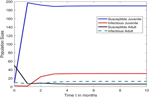shows that the juvenile-adult SIR disease invades both the juvenile and adult populations via a positive fixed point attractor. That is, under the Beverton-Holt recruitment function, the juvenile-adult disease-free equilibrium dynamics drives the disease dynamics when ${\mathcal{R}}_d>1$ and ${\mathcal{R}}_0>1$. In Figure 2, the fraction of juveniles that die per unit interval, $d_J$, is larger than the fraction of adults, $d_A$. However, due to the large intrinsic growth rate of the Beverton-Holt recruitment (or birth) function of adults into the susceptible juvenile class per unit time interval, r = 200, $S^A$ is smaller than $S^J$ and $I^A$ is smaller than $I^J$. In Figure 2, at the onset of the juvenile-adult SIR infection, $I^J$ is smaller than $S^J$ and $I^A$ is smaller than $S^A$. However, due to the influx of the new recruits into the juvenile susceptible class, $I^J$ remains smaller than $S^J$ while $I^A$ increases to values larger than $S^A$ after about 1.4 months of the juvenile-adult SIR infection. Our simulations with other positive initial population numbers lead to the same positive fixed point attractor as in Figure 2.

Figure 2. With Beverton-Holt recruitment and initial population numbers $(S_0^J,I_0^J,R_0^J,S_0^A,I_0^A,R_0^A)=(50,10,5,10,2,1),$ the disease-free fixed point population dynamics drives the SIR disease dynamics and the disease invades both juvenile and adult populations via a fixed point attractor when ${\mathcal{R}}_d=19.678$ and ${\mathcal{R}}_0=30.04$, where ${\theta }_J={\theta }_A=0.5$, ${\eta }_J={\eta }_A={\text{β}}_J={\text{β}}_A=\text{β}=0.9$, ${\gamma }_J={\gamma }_A=0.01$, r = 200, $b=1,d_J=0.8,$ $d_A=0.78$ and m = 0.3.

Next, we consider Model (1(1) $\left.\begin{array}{rl}{S}_{t+1}^J& =g\left(N_t^A\right)+{\hat{d}}_J\hat{m}{S}_t^J\left({\theta }_J{\varphi }_J\left(I_t^J\right)+\left(1-{\theta }_J\right){\varphi }_J\left(I_t^A\right)\right)\\ I_{t+1}^J& ={\hat{d}}_J\hat{m}{S}_t^J\left({\theta }_J{\hat{\varphi }}_J\left(I_t^J\right)+\left(1-{\theta }_J\right){\hat{\varphi }}_J\left(I_t^A\right)\right)+{\hat{d}}_J\hat{m}{\hat{\gamma }}_J{I}_t^J\\ R_{t+1}^J& ={\hat{d}}_J\hat{m}{\gamma }_J{I}_t^J+{\hat{d}}_J\hat{m}{R}_t^J\\ S_{t+1}^A& ={\hat{d}}_A\left(m{S}_t^J+S_t^A\right)\left({\theta }_A{\varphi }_A\left(I_t^J\right)+\left(1-{\theta }_A\right){\varphi }_A\left(I_t^A\right)\right)\\ I_{t+1}^A& ={\hat{d}}_A\left(m{S}_t^J+S_t^A\right)\left({\theta }_A{\hat{\varphi }}_A\left(I_t^J\right)+\left(1-{\theta }_A\right){\hat{\varphi }}_A\left(I_t^A\right)\right)+{\hat{d}}_A{\hat{\gamma }}_A\left(m{I}_t^J+I_t^A\right)\\ R_{t+1}^A& ={\hat{d}}_A{\gamma }_A\left(m{I}_t^J+I_t^A\right)+{\hat{d}}_A\left(m{R}_t^J+R_t^A\right)\end{array}\right\}$(1) ) with Ricker recruitment $g\left(N_t^A\right)=r{N}_t^A\exp \left(-b{N}_t^A\right),$ where the model's unit of time is a month. To illustrate the impact of increasing ${\mathcal{R}}_0$ from values less than 1 to values greater than 1, as in [8,35], we let $d_J=0.98,$ $d_A=0.9$, and keep all the model parameters fixed at their current values in Figure 2 while ${\text{β}}_J={\text{β}}_A=\text{β}$ varies between 0.5 and 1.0. 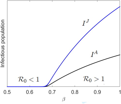With our choice of parameters, the juvenile-adult disease-free model, Model (2(2) $\left.\begin{array}{rl}{S}_{t+1}^J& =g\left(S_t^A\right)+\left(1-d_J\right)\left(1-m\right)S_t^J\\ S_{t+1}^A& =\left(1-d_A\right)\left(m{S}_t^J+S_t^A\right)\end{array}\right\}$(2) ), has a globally asymptotically stable DFE (see Figure 1). With initial condition $\left(S_0^J,I_0^J,R_0^J,S_0^A,I_0^A,R_0^A\right)=\left(100,10,5,100,10,5\right),$ as the infection rate β increases from zero to values greater than $\text{β}=0.676$, we show in Figure 3 that ${\mathcal{R}}_0$ increases from values less than 1 (disease extinction) to values greater than 1 (disease persistence), and the disease invades both the juvenile and adult populations via a positive fixed point attractor when ${\mathcal{R}}_0>1$. That is, as in Figure 2, under the Ricker recruitment function, the juvenile-adult disease-free equilibrium dynamics drives the juvenile-adult disease dynamics when ${\mathcal{R}}_0>1$. The DFE is stable and the disease does not invade the juvenile-adult population when ${\mathcal{R}}_0<1$ (see Figure 3). Our simulations with other positive initial population numbers lead to the same dynamics as in Figure 3.

Figure 3. With Ricker recruitment and initial population numbers $(S_0^J,I_0^J,R_0^J,S_0^A,I_0^A,R_0^A)=(100,10,5,100,10,5)$, ${\mathcal{R}}_0$ increases from values less than 1 ($\text{β}<0.676$, disease extinction) to values greater than 1 (disease persistence), and the disease invades both the juvenile and adult populations via a positive fixed point attractor when ${\mathcal{R}}_0>1$ ($\text{β}>0.676$), where r = 200, $b=1,d_J=0.98,$ $d_A=0.9$ and $m=0.3,$ ${\theta }_J={\theta }_A=0.5$, ${\eta }_J={\eta }_A=0.9$, ${\gamma }_J={\gamma }_A=0.01$.

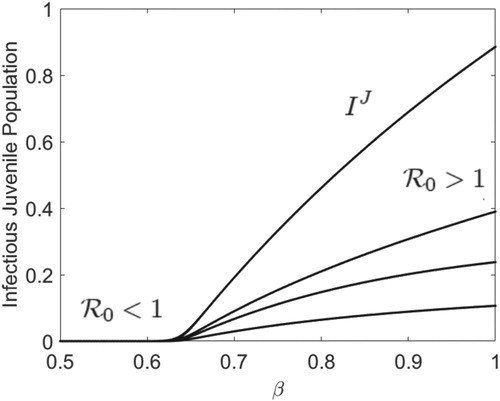
Next, we take r = 400 and keep all the parameters fixed at their current values in Figure 4 while β varies between 0.5 and 1.0. With our choice of parameters, the juvenile-adult disease-free model, Model (2(2) $\left.\begin{array}{rl}{S}_{t+1}^J& =g\left(S_t^A\right)+\left(1-d_J\right)\left(1-m\right)S_t^J\\ S_{t+1}^A& =\left(1-d_A\right)\left(m{S}_t^J+S_t^A\right)\end{array}\right\}$(2) ), has an asymptotically stable period 4 population cycle (see Figure 1). As β increases from zero to values larger than $\text{β}\approx 0.641$ where ${\mathcal{R}}_0\approx 1$, we show in Figure 4 that ${\mathcal{R}}_0$ increases from values less than 1 to values larger than 1 and the disease invades both the juvenile and adult (not shown) populations via a period 4 attractor when ${\mathcal{R}}_0>1$. That is, as in Figure 2, the juvenile-adult disease-free periodic dynamics drives the juvenile-adult disease dynamics when ${\mathcal{R}}_0>1$. The juvenile-adult disease-free period 4 population cycle is stable and the disease does not invade the juvenile-adult population when ${\mathcal{R}}_0<1$ (see Figure 4). Other positive initial population numbers numerically lead to the same dynamics. Thus, our age-structured model exhibits the same dynamical behaviour as the SIR model without age-structure [35].

Figure 4. With Ricker recruitment and initial population numbers $(S_0^J,I_0^J,R_0^J,S_0^A,I_0^A,R_0^A)=(100,10,5,100,10,5)$, the disease-free period 4 population cycle drives the SIR disease dynamics and the disease invades both juvenile and adult (not shown) populations via a period 4 attractor when ${\mathcal{R}}_0>1$. However, the disease does not invade the population when ${\mathcal{R}}_0<1$, where r = 400 and all the other parameters are fixed at their values in Figure 3 while β varies between 0.5 and 1.0. Here, ${\mathcal{R}}_0<1$ when $\text{β}<0.641$, ${\mathcal{R}}_0\approx 1$ when $\text{β}\approx 0.641$, and ${\mathcal{R}}_0>1$ when $\text{β}>0.641$.

3. Juvenile-Adult discrete-time ISAv model

Infectious salmon anemia (ISA), a disease of Atlantic salmon (Salmo salar), is caused by an orthomyxovirus and affects mainly fish maintained in marine water or exposed to the sea. ISA is systemic and lethal, and it is characterized by severe anemia and hemorrhages in several organs. ISA is a disease of great economic impact for the salmon industry, and has caused significant mortality among salmon farms in Northern Europe, Canada, Maine, and Chile. Following recent detection and outbreak of the ISA virus, Chile's National Fisheries and Aquaculture Service officially declared farming centre Rowlett 749 in the Patagonia Aisen region of Chile as a centre with an ISA virus outbreak (http://www.promedmail.org/).

Due to the severity of the disease, the European Union includes ISA in its list of the most dangerous diseases of fish, and it is one of just 10 virus infections of finfish that is reportable to the World Organization for Animal Health [12,19,28,38]. Currently, there are no treatment options available for ISA. Typically, ISA disease outbreaks have been managed through a combination of regulatory measures and husbandry practices, including restricted movements of fish between farms, enforced slaughtering, use of all-in–all-out programmes at farms, and disinfection of slaughterhouses and processing plants.

In [35], van den Driessche and Yakubu introduced a discrete-time model of infectious salmon anemia virus (ISAv) without age structure. Here, we introduce a juvenile-adult discrete-time ISAv model. We assume that at each time $t\in \{0,1,2,\dots \}$, each live salmon is either susceptible juvenile (age < 2 years), $S_t^J$, or susceptible adult ($\mathrm{a}\mathrm{g}\mathrm{e}\ge 2$ years), $S_t^A$, or infectious juvenile ($\mathrm{a}\mathrm{g}\mathrm{e}<2$ years and infected with ISA disease), $I_t^J$, or infectious adult ($\mathrm{a}\mathrm{g}\mathrm{e}\ge 2$ years and infected with ISA disease), $I_t^A$. That is, we let $S_t^{\mathrm{\Lambda }}$, $I_t^{\mathrm{\Lambda }}$, and $N_t^{\mathrm{\Lambda }}=S_t^{\mathrm{\Lambda }}$ + $I_t^{\mathrm{\Lambda }}$ respectively denote the population size of susceptible, infectious, and total population of live juvenile (respectively, adult) salmon at each time t when $\mathrm{\Lambda }=J$ (respectively, when $\mathrm{\Lambda }=A)$. Once infected, salmon do not recover from the ISAv disease. Thus, we use an SI juvenile-adult epidemic model with no recovery class to describe the salmon population [1]. At each time $t\in \{0,1,2,\dots \}$, we denote the virus population size by $V_t$.

Melville and Griffiths, in [27], observed absence of a vertical transmission route for ISAv infection from individual ISA infected Atlantic salmon. In a 2014 paper [25], evidence of mother-to-offspring vertical transmission of the ISAv was demonstrated. For simplicity, as in [35], we assume that infectious adult salmon cannot reproduce. That is, we assume that only the susceptible adult salmon population reproduce and all newborn salmon are susceptible juveniles. Also, per unit time interval, $d_J\in (0,1)$ (respectively, $d_A\in (0,1)$) is the fraction of juvenile (respectively, adult) salmon that die of natural causes, ${\hat{d}}_J=(1-d_J)$ (respectively, ${\hat{d}}_A=(1-d_A)$) is the fraction of juvenile (respectively, adult) salmon that do not die due to natural mortality, ${\mu }_J\in (0,1)$ (respectively, ${\mu }_A\in (0,1)$) is the fraction of juveniles (respectively, adults) that die due to ISA, ${\hat{\mu }}_J=(1-{\mu }_J)$ (respectively, ${\hat{\mu }}_A=(1-{\mu }_A)$) is the fraction of ISA infectious juvenile (respectively, adult) salmon that survive the disease, $d_V\in (0,1)$ is the constant fraction of virus that is cleared and ${\hat{d}}_V=(1-d_V)$ is the fraction of virus that survive. As in [35], we assume that $d_A\le d_J$.

At each time $t\in \{0,1,2,\dots \},$ we assume that a fraction of juvenile susceptible salmon, ${\theta }_{1J}\in (0,1)$, become infected from direct contact with infectious juvenile salmon with probability ${\hat{\varphi }}_J\left(I_t^J\right)=(1-{\varphi }_J(I_t^J\left)\right)$, a fraction of juvenile susceptible salmon, ${\theta }_{2J}\in (0,1)$, become infected from direct contact with infectious adult salmon with probability ${\hat{\varphi }}_J\left(I_t^A\right)=(1-{\varphi }_J(I_t^A\left)\right)$ and the remaining juvenile susceptible salmon, ${\theta }_{3J}=(1-({\theta }_{1J}+{\theta }_{2J}\left)\right)\in (0,1)$, become infected via contact with the ISA virus with probability ${\hat{\varphi }}_V\left(V_t\right)=(1-{\varphi }_V(V_t\left)\right)$, where the ‘escape’ functions ${\varphi }_J,{\varphi }_V:{\mathbb{R}}_{+}\to [0,1]$ are nonlinear decreasing smooth concave up functions with ${\varphi }_J\left(0\right)={\varphi }_V\left(0\right)=1$, ${\varphi }_J^{\mathrm{\prime }}<0$, ${\varphi }_V^{\mathrm{\prime }}<0$, ${\varphi }_J^{\mathrm{\prime }\mathrm{\prime }}>0$ and ${\varphi }_V^{\mathrm{\prime }\mathrm{\prime }}>0$. Similarly, at each time $t\in \{0,1,2,\dots \},$ we assume that a fraction of adult susceptible salmon, ${\theta }_{1A}\in (0,1)$, become infected from direct contact with infectious juvenile salmon with probability ${\hat{\varphi }}_A\left(I_t^J\right)=(1-{\varphi }_A(I_t^J\left)\right)$, a fraction of adult susceptible salmon, ${\theta }_{2A}\in (0,1)$, become infected from direct contact with infectious adult salmon with probability ${\hat{\varphi }}_A\left(I_t^A\right)=(1-{\varphi }_A(I_t^A\left)\right)$ and the remaining adult susceptible salmon, ${\theta }_{3A}=(1-({\theta }_{1A}+{\theta }_{2A}\left)\right)\in (0,1)$, become infected via contact with the ISA virus with probability ${\hat{\varphi }}_V\left(V_t\right)=(1-{\varphi }_V(V_t\left)\right)$, where the ‘escape’ function ${\varphi }_A:{\mathbb{R}}_{+}\to [0,1]$ is a nonlinear decreasing smooth concave up function with ${\varphi }_A\left(0\right)=1$, ${\varphi }_A^{\mathrm{\prime }}<0$ and ${\varphi }_A^{\mathrm{\prime }\mathrm{\prime }}>0$. As in Model (1(1) $\left.\begin{array}{rl}{S}_{t+1}^J& =g\left(N_t^A\right)+{\hat{d}}_J\hat{m}{S}_t^J\left({\theta }_J{\varphi }_J\left(I_t^J\right)+\left(1-{\theta }_J\right){\varphi }_J\left(I_t^A\right)\right)\\ I_{t+1}^J& ={\hat{d}}_J\hat{m}{S}_t^J\left({\theta }_J{\hat{\varphi }}_J\left(I_t^J\right)+\left(1-{\theta }_J\right){\hat{\varphi }}_J\left(I_t^A\right)\right)+{\hat{d}}_J\hat{m}{\hat{\gamma }}_J{I}_t^J\\ R_{t+1}^J& ={\hat{d}}_J\hat{m}{\gamma }_J{I}_t^J+{\hat{d}}_J\hat{m}{R}_t^J\\ S_{t+1}^A& ={\hat{d}}_A\left(m{S}_t^J+S_t^A\right)\left({\theta }_A{\varphi }_A\left(I_t^J\right)+\left(1-{\theta }_A\right){\varphi }_A\left(I_t^A\right)\right)\\ I_{t+1}^A& ={\hat{d}}_A\left(m{S}_t^J+S_t^A\right)\left({\theta }_A{\hat{\varphi }}_A\left(I_t^J\right)+\left(1-{\theta }_A\right){\hat{\varphi }}_A\left(I_t^A\right)\right)+{\hat{d}}_A{\hat{\gamma }}_A\left(m{I}_t^J+I_t^A\right)\\ R_{t+1}^A& ={\hat{d}}_A{\gamma }_A\left(m{I}_t^J+I_t^A\right)+{\hat{d}}_A\left(m{R}_t^J+R_t^A\right)\end{array}\right\}$(1) ), we assume that the probability of exposure of an individual susceptible salmon to multiple infection pathways is low, so it can be ignored.

As in [35], we account for virus shedding in our model. During each time interval, ${\delta }_J{I}_t^J$ and ${\delta }_A{I}_t^A$ are respectively the population of virus shed by the juvenile and adult populations, where ${\delta }_J,{\delta }_A>0$. As in Section 2, in each time interval, a constant fraction of juvenile salmon, m $\in (0,1)$, mature to adulthood and the fraction of juvenile salmon, $\hat{m}=(1-m)$, remain in the juvenile class.

As in Model (1(1) $\left.\begin{array}{rl}{S}_{t+1}^J& =g\left(N_t^A\right)+{\hat{d}}_J\hat{m}{S}_t^J\left({\theta }_J{\varphi }_J\left(I_t^J\right)+\left(1-{\theta }_J\right){\varphi }_J\left(I_t^A\right)\right)\\ I_{t+1}^J& ={\hat{d}}_J\hat{m}{S}_t^J\left({\theta }_J{\hat{\varphi }}_J\left(I_t^J\right)+\left(1-{\theta }_J\right){\hat{\varphi }}_J\left(I_t^A\right)\right)+{\hat{d}}_J\hat{m}{\hat{\gamma }}_J{I}_t^J\\ R_{t+1}^J& ={\hat{d}}_J\hat{m}{\gamma }_J{I}_t^J+{\hat{d}}_J\hat{m}{R}_t^J\\ S_{t+1}^A& ={\hat{d}}_A\left(m{S}_t^J+S_t^A\right)\left({\theta }_A{\varphi }_A\left(I_t^J\right)+\left(1-{\theta }_A\right){\varphi }_A\left(I_t^A\right)\right)\\ I_{t+1}^A& ={\hat{d}}_A\left(m{S}_t^J+S_t^A\right)\left({\theta }_A{\hat{\varphi }}_A\left(I_t^J\right)+\left(1-{\theta }_A\right){\hat{\varphi }}_A\left(I_t^A\right)\right)+{\hat{d}}_A{\hat{\gamma }}_A\left(m{I}_t^J+I_t^A\right)\\ R_{t+1}^A& ={\hat{d}}_A{\gamma }_A\left(m{I}_t^J+I_t^A\right)+{\hat{d}}_A\left(m{R}_t^J+R_t^A\right)\end{array}\right\}$(1) ), our discrete-time juvenile-adult ISAv model implicitly assumes three distinct temporal phases. At the end of each time interval, juvenile and adult susceptible salmon populations become infectious, then juvenile salmon population mature to adulthood, a fraction of juvenile and adult infectious salmon die, shedding occurs; a fraction of each juvenile and adult salmon class is removed (natural death and virus clearing); and adult susceptible salmon populations reproduce into the juvenile susceptible class. Taking into account the temporal ordering of events, we obtain the following juvenile-adult ISAv model. (6) $\left.\begin{array}{rl}{S}_{t+1}^J& =g\left(S_t^A\right)+{\hat{d}}_J\hat{m}{S}_t^J\left({\theta }_{1J}{\varphi }_J\left(I_t^J\right)+{\theta }_{2J}{\varphi }_J\left(I_t^A\right)+{\theta }_{3J}{\varphi }_V\left(V_t\right)\right)\\ I_{t+1}^J& ={\hat{d}}_J\hat{m}{S}_t^J{\hat{\mathrm{\Phi }}}_J\left(I_t^J,I_t^A,V_t\right)+{\hat{d}}_J\hat{m}{\hat{\mu }}_J{I}_t^J\\ S_{t+1}^A& ={\hat{d}}_A\left(m{S}_t^J+S_t^A\right)\left({\theta }_{1A}{\varphi }_A\left(I_t^J\right)+{\theta }_{2A}{\varphi }_A\left(I_t^A\right)+{\theta }_{3A}{\varphi }_V\left(V_t\right)\right)\\ I_{t+1}^A& ={\hat{d}}_A\left(m{S}_t^J+S_t^A\right){\hat{\mathrm{\Phi }}}_A\left(I_t^J,I_t^A,V_t\right)+{\hat{d}}_A{\hat{\mu }}_A\left(m{I}_t^J+I_t^A\right)\\ V_{t+1}& ={\hat{d}}_V\left(V_t+{\delta }_J{I}_t^J+{\delta }_A{I}_t^A\right)\end{array}\right\}$(6) where $\begin{array}{rl}{\hat{\mathrm{\Phi }}}_J\left(I_t^J,I_t^A,V_t\right)& =\left({\theta }_{1J}{\hat{\varphi }}_J\left(I_t^J\right)+{\theta }_{2J}{\hat{\varphi }}_J\left(I_t^A\right)+{\theta }_{3J}{\hat{\varphi }}_V\left(V_t\right)\right),\\ {\hat{\mathrm{\Phi }}}_A\left(I_t^J,I_t^A,V_t\right)& =\left({\theta }_{1A}{\hat{\varphi }}_A\left(I_t^J\right)+{\theta }_{2A}{\hat{\varphi }}_A\left(I_t^A\right)+{\theta }_{3A}{\hat{\varphi }}_V\left(V_t\right)\right),\end{array}$ and $t=0,1,2,\dots$. Model (6(6) $\left.\begin{array}{rl}{S}_{t+1}^J& =g\left(S_t^A\right)+{\hat{d}}_J\hat{m}{S}_t^J\left({\theta }_{1J}{\varphi }_J\left(I_t^J\right)+{\theta }_{2J}{\varphi }_J\left(I_t^A\right)+{\theta }_{3J}{\varphi }_V\left(V_t\right)\right)\\ I_{t+1}^J& ={\hat{d}}_J\hat{m}{S}_t^J{\hat{\mathrm{\Phi }}}_J\left(I_t^J,I_t^A,V_t\right)+{\hat{d}}_J\hat{m}{\hat{\mu }}_J{I}_t^J\\ S_{t+1}^A& ={\hat{d}}_A\left(m{S}_t^J+S_t^A\right)\left({\theta }_{1A}{\varphi }_A\left(I_t^J\right)+{\theta }_{2A}{\varphi }_A\left(I_t^A\right)+{\theta }_{3A}{\varphi }_V\left(V_t\right)\right)\\ I_{t+1}^A& ={\hat{d}}_A\left(m{S}_t^J+S_t^A\right){\hat{\mathrm{\Phi }}}_A\left(I_t^J,I_t^A,V_t\right)+{\hat{d}}_A{\hat{\mu }}_A\left(m{I}_t^J+I_t^A\right)\\ V_{t+1}& ={\hat{d}}_V\left(V_t+{\delta }_J{I}_t^J+{\delta }_A{I}_t^A\right)\end{array}\right\}$(6) ) has initial conditions $(S_0^J,I_0^J,S_0^A,I_0^A,V_0)\in {\mathbb{R}}_{+}^5$.

When there is no age-structure and the juvenile populations are missing $(\hat{m}=1)$, Model (6(6) $\left.\begin{array}{rl}{S}_{t+1}^J& =g\left(S_t^A\right)+{\hat{d}}_J\hat{m}{S}_t^J\left({\theta }_{1J}{\varphi }_J\left(I_t^J\right)+{\theta }_{2J}{\varphi }_J\left(I_t^A\right)+{\theta }_{3J}{\varphi }_V\left(V_t\right)\right)\\ I_{t+1}^J& ={\hat{d}}_J\hat{m}{S}_t^J{\hat{\mathrm{\Phi }}}_J\left(I_t^J,I_t^A,V_t\right)+{\hat{d}}_J\hat{m}{\hat{\mu }}_J{I}_t^J\\ S_{t+1}^A& ={\hat{d}}_A\left(m{S}_t^J+S_t^A\right)\left({\theta }_{1A}{\varphi }_A\left(I_t^J\right)+{\theta }_{2A}{\varphi }_A\left(I_t^A\right)+{\theta }_{3A}{\varphi }_V\left(V_t\right)\right)\\ I_{t+1}^A& ={\hat{d}}_A\left(m{S}_t^J+S_t^A\right){\hat{\mathrm{\Phi }}}_A\left(I_t^J,I_t^A,V_t\right)+{\hat{d}}_A{\hat{\mu }}_A\left(m{I}_t^J+I_t^A\right)\\ V_{t+1}& ={\hat{d}}_V\left(V_t+{\delta }_J{I}_t^J+{\delta }_A{I}_t^A\right)\end{array}\right\}$(6) ) reduces to the unstructured ISAv model in [35, Section 4], where $g\left(S_t\right)$ is the recruitment function of the susceptibles (adults) into the susceptibles class per unit time interval.

Proceeding as in the proof of Theorem 2.1, the following theorem on well-posedness of Model (6(6) $\left.\begin{array}{rl}{S}_{t+1}^J& =g\left(S_t^A\right)+{\hat{d}}_J\hat{m}{S}_t^J\left({\theta }_{1J}{\varphi }_J\left(I_t^J\right)+{\theta }_{2J}{\varphi }_J\left(I_t^A\right)+{\theta }_{3J}{\varphi }_V\left(V_t\right)\right)\\ I_{t+1}^J& ={\hat{d}}_J\hat{m}{S}_t^J{\hat{\mathrm{\Phi }}}_J\left(I_t^J,I_t^A,V_t\right)+{\hat{d}}_J\hat{m}{\hat{\mu }}_J{I}_t^J\\ S_{t+1}^A& ={\hat{d}}_A\left(m{S}_t^J+S_t^A\right)\left({\theta }_{1A}{\varphi }_A\left(I_t^J\right)+{\theta }_{2A}{\varphi }_A\left(I_t^A\right)+{\theta }_{3A}{\varphi }_V\left(V_t\right)\right)\\ I_{t+1}^A& ={\hat{d}}_A\left(m{S}_t^J+S_t^A\right){\hat{\mathrm{\Phi }}}_A\left(I_t^J,I_t^A,V_t\right)+{\hat{d}}_A{\hat{\mu }}_A\left(m{I}_t^J+I_t^A\right)\\ V_{t+1}& ={\hat{d}}_V\left(V_t+{\delta }_J{I}_t^J+{\delta }_A{I}_t^A\right)\end{array}\right\}$(6) ) is immediate.

Theorem 3.1

In Model (6(6) $\left.\begin{array}{rl}{S}_{t+1}^J& =g\left(S_t^A\right)+{\hat{d}}_J\hat{m}{S}_t^J\left({\theta }_{1J}{\varphi }_J\left(I_t^J\right)+{\theta }_{2J}{\varphi }_J\left(I_t^A\right)+{\theta }_{3J}{\varphi }_V\left(V_t\right)\right)\\ I_{t+1}^J& ={\hat{d}}_J\hat{m}{S}_t^J{\hat{\mathrm{\Phi }}}_J\left(I_t^J,I_t^A,V_t\right)+{\hat{d}}_J\hat{m}{\hat{\mu }}_J{I}_t^J\\ S_{t+1}^A& ={\hat{d}}_A\left(m{S}_t^J+S_t^A\right)\left({\theta }_{1A}{\varphi }_A\left(I_t^J\right)+{\theta }_{2A}{\varphi }_A\left(I_t^A\right)+{\theta }_{3A}{\varphi }_V\left(V_t\right)\right)\\ I_{t+1}^A& ={\hat{d}}_A\left(m{S}_t^J+S_t^A\right){\hat{\mathrm{\Phi }}}_A\left(I_t^J,I_t^A,V_t\right)+{\hat{d}}_A{\hat{\mu }}_A\left(m{I}_t^J+I_t^A\right)\\ V_{t+1}& ={\hat{d}}_V\left(V_t+{\delta }_J{I}_t^J+{\delta }_A{I}_t^A\right)\end{array}\right\}$(6) ), for each time $t\in \{1,2,\dots \},$ $(S_t^J,I_t^J,S_t^A,I_t^A,V_t)\in {\mathbb{R}}_{+}^5$ and there is no unbounded population growth whenever $(S_0^J,I_0^J,S_0^A,I_0^A,V_0)\in {\mathbb{R}}_{+}^5$.

Proof.

Clearly, $(S_0^J,I_0^J,S_0^A,I_0^A,V_0)\in {\mathbb{R}}_{+}^5$ implies $(S_t^J,I_t^J,S_t^A,I_t^A,V_t)\in {\mathbb{R}}_{+}^5$ for each $t\ge 0$. Using $d_A\le d_J$, we obtain that $N_{t+1}^J\le g\left(S_t^A\right)+{\hat{d}}_J\hat{m}{N}_t^J$ and $N_{t+1}^A\le {\hat{d}}_A\left(m{N}_t^J+N_t^A\right).$ Consequently, $N_{t+1}\le g\left(S_t^A\right)+{\hat{d}}_A{N}_t.$ Since $g\left(S_t^A\right)=S_t^{A}h\left(S_t^A\right)\ge 0$ is a smooth function and $\underset{S_t^A\to \mathrm{\infty }}{lim}h\left(S_t^A\right)=0,$ we proceed as in the proof of Theorem 2.1 to establish the boundedness of the salmon population. From the last equation of Model (6(6) $\left.\begin{array}{rl}{S}_{t+1}^J& =g\left(S_t^A\right)+{\hat{d}}_J\hat{m}{S}_t^J\left({\theta }_{1J}{\varphi }_J\left(I_t^J\right)+{\theta }_{2J}{\varphi }_J\left(I_t^A\right)+{\theta }_{3J}{\varphi }_V\left(V_t\right)\right)\\ I_{t+1}^J& ={\hat{d}}_J\hat{m}{S}_t^J{\hat{\mathrm{\Phi }}}_J\left(I_t^J,I_t^A,V_t\right)+{\hat{d}}_J\hat{m}{\hat{\mu }}_J{I}_t^J\\ S_{t+1}^A& ={\hat{d}}_A\left(m{S}_t^J+S_t^A\right)\left({\theta }_{1A}{\varphi }_A\left(I_t^J\right)+{\theta }_{2A}{\varphi }_A\left(I_t^A\right)+{\theta }_{3A}{\varphi }_V\left(V_t\right)\right)\\ I_{t+1}^A& ={\hat{d}}_A\left(m{S}_t^J+S_t^A\right){\hat{\mathrm{\Phi }}}_A\left(I_t^J,I_t^A,V_t\right)+{\hat{d}}_A{\hat{\mu }}_A\left(m{I}_t^J+I_t^A\right)\\ V_{t+1}& ={\hat{d}}_V\left(V_t+{\delta }_J{I}_t^J+{\delta }_A{I}_t^A\right)\end{array}\right\}$(6) ), $V_{t+1}={\hat{d}}_V\left(V_t+{\delta }_J{I}_t^J+{\delta }_A{I}_t^A\right)$ where ${\hat{d}}_V\in (0,1)$. Therefore, the boundedness of the salmon population guarantees that the virus population is also bounded and there is no unbounded population growth in Model (6(6) $\left.\begin{array}{rl}{S}_{t+1}^J& =g\left(S_t^A\right)+{\hat{d}}_J\hat{m}{S}_t^J\left({\theta }_{1J}{\varphi }_J\left(I_t^J\right)+{\theta }_{2J}{\varphi }_J\left(I_t^A\right)+{\theta }_{3J}{\varphi }_V\left(V_t\right)\right)\\ I_{t+1}^J& ={\hat{d}}_J\hat{m}{S}_t^J{\hat{\mathrm{\Phi }}}_J\left(I_t^J,I_t^A,V_t\right)+{\hat{d}}_J\hat{m}{\hat{\mu }}_J{I}_t^J\\ S_{t+1}^A& ={\hat{d}}_A\left(m{S}_t^J+S_t^A\right)\left({\theta }_{1A}{\varphi }_A\left(I_t^J\right)+{\theta }_{2A}{\varphi }_A\left(I_t^A\right)+{\theta }_{3A}{\varphi }_V\left(V_t\right)\right)\\ I_{t+1}^A& ={\hat{d}}_A\left(m{S}_t^J+S_t^A\right){\hat{\mathrm{\Phi }}}_A\left(I_t^J,I_t^A,V_t\right)+{\hat{d}}_A{\hat{\mu }}_A\left(m{I}_t^J+I_t^A\right)\\ V_{t+1}& ={\hat{d}}_V\left(V_t+{\delta }_J{I}_t^J+{\delta }_A{I}_t^A\right)\end{array}\right\}$(6) ).

3.1. ${\mathcal{R}}_0$ for Juvenile-Adult ISAv model

Models (1(1) $\left.\begin{array}{rl}{S}_{t+1}^J& =g\left(N_t^A\right)+{\hat{d}}_J\hat{m}{S}_t^J\left({\theta }_J{\varphi }_J\left(I_t^J\right)+\left(1-{\theta }_J\right){\varphi }_J\left(I_t^A\right)\right)\\ I_{t+1}^J& ={\hat{d}}_J\hat{m}{S}_t^J\left({\theta }_J{\hat{\varphi }}_J\left(I_t^J\right)+\left(1-{\theta }_J\right){\hat{\varphi }}_J\left(I_t^A\right)\right)+{\hat{d}}_J\hat{m}{\hat{\gamma }}_J{I}_t^J\\ R_{t+1}^J& ={\hat{d}}_J\hat{m}{\gamma }_J{I}_t^J+{\hat{d}}_J\hat{m}{R}_t^J\\ S_{t+1}^A& ={\hat{d}}_A\left(m{S}_t^J+S_t^A\right)\left({\theta }_A{\varphi }_A\left(I_t^J\right)+\left(1-{\theta }_A\right){\varphi }_A\left(I_t^A\right)\right)\\ I_{t+1}^A& ={\hat{d}}_A\left(m{S}_t^J+S_t^A\right)\left({\theta }_A{\hat{\varphi }}_A\left(I_t^J\right)+\left(1-{\theta }_A\right){\hat{\varphi }}_A\left(I_t^A\right)\right)+{\hat{d}}_A{\hat{\gamma }}_A\left(m{I}_t^J+I_t^A\right)\\ R_{t+1}^A& ={\hat{d}}_A{\gamma }_A\left(m{I}_t^J+I_t^A\right)+{\hat{d}}_A\left(m{R}_t^J+R_t^A\right)\end{array}\right\}$(1) ) and (6(6) $\left.\begin{array}{rl}{S}_{t+1}^J& =g\left(S_t^A\right)+{\hat{d}}_J\hat{m}{S}_t^J\left({\theta }_{1J}{\varphi }_J\left(I_t^J\right)+{\theta }_{2J}{\varphi }_J\left(I_t^A\right)+{\theta }_{3J}{\varphi }_V\left(V_t\right)\right)\\ I_{t+1}^J& ={\hat{d}}_J\hat{m}{S}_t^J{\hat{\mathrm{\Phi }}}_J\left(I_t^J,I_t^A,V_t\right)+{\hat{d}}_J\hat{m}{\hat{\mu }}_J{I}_t^J\\ S_{t+1}^A& ={\hat{d}}_A\left(m{S}_t^J+S_t^A\right)\left({\theta }_{1A}{\varphi }_A\left(I_t^J\right)+{\theta }_{2A}{\varphi }_A\left(I_t^A\right)+{\theta }_{3A}{\varphi }_V\left(V_t\right)\right)\\ I_{t+1}^A& ={\hat{d}}_A\left(m{S}_t^J+S_t^A\right){\hat{\mathrm{\Phi }}}_A\left(I_t^J,I_t^A,V_t\right)+{\hat{d}}_A{\hat{\mu }}_A\left(m{I}_t^J+I_t^A\right)\\ V_{t+1}& ={\hat{d}}_V\left(V_t+{\delta }_J{I}_t^J+{\delta }_A{I}_t^A\right)\end{array}\right\}$(6) ) share the same juvenile-adult disease-free system when $I_t^J=I_t^A=V_t=0$, namely Model (2(2) $\left.\begin{array}{rl}{S}_{t+1}^J& =g\left(S_t^A\right)+\left(1-d_J\right)\left(1-m\right)S_t^J\\ S_{t+1}^A& =\left(1-d_A\right)\left(m{S}_t^J+S_t^A\right)\end{array}\right\}$(2) ). As in Model (1(1) $\left.\begin{array}{rl}{S}_{t+1}^J& =g\left(N_t^A\right)+{\hat{d}}_J\hat{m}{S}_t^J\left({\theta }_J{\varphi }_J\left(I_t^J\right)+\left(1-{\theta }_J\right){\varphi }_J\left(I_t^A\right)\right)\\ I_{t+1}^J& ={\hat{d}}_J\hat{m}{S}_t^J\left({\theta }_J{\hat{\varphi }}_J\left(I_t^J\right)+\left(1-{\theta }_J\right){\hat{\varphi }}_J\left(I_t^A\right)\right)+{\hat{d}}_J\hat{m}{\hat{\gamma }}_J{I}_t^J\\ R_{t+1}^J& ={\hat{d}}_J\hat{m}{\gamma }_J{I}_t^J+{\hat{d}}_J\hat{m}{R}_t^J\\ S_{t+1}^A& ={\hat{d}}_A\left(m{S}_t^J+S_t^A\right)\left({\theta }_A{\varphi }_A\left(I_t^J\right)+\left(1-{\theta }_A\right){\varphi }_A\left(I_t^A\right)\right)\\ I_{t+1}^A& ={\hat{d}}_A\left(m{S}_t^J+S_t^A\right)\left({\theta }_A{\hat{\varphi }}_A\left(I_t^J\right)+\left(1-{\theta }_A\right){\hat{\varphi }}_A\left(I_t^A\right)\right)+{\hat{d}}_A{\hat{\gamma }}_A\left(m{I}_t^J+I_t^A\right)\\ R_{t+1}^A& ={\hat{d}}_A{\gamma }_A\left(m{I}_t^J+I_t^A\right)+{\hat{d}}_A\left(m{R}_t^J+R_t^A\right)\end{array}\right\}$(1) ), in Model (6(6) $\left.\begin{array}{rl}{S}_{t+1}^J& =g\left(S_t^A\right)+{\hat{d}}_J\hat{m}{S}_t^J\left({\theta }_{1J}{\varphi }_J\left(I_t^J\right)+{\theta }_{2J}{\varphi }_J\left(I_t^A\right)+{\theta }_{3J}{\varphi }_V\left(V_t\right)\right)\\ I_{t+1}^J& ={\hat{d}}_J\hat{m}{S}_t^J{\hat{\mathrm{\Phi }}}_J\left(I_t^J,I_t^A,V_t\right)+{\hat{d}}_J\hat{m}{\hat{\mu }}_J{I}_t^J\\ S_{t+1}^A& ={\hat{d}}_A\left(m{S}_t^J+S_t^A\right)\left({\theta }_{1A}{\varphi }_A\left(I_t^J\right)+{\theta }_{2A}{\varphi }_A\left(I_t^A\right)+{\theta }_{3A}{\varphi }_V\left(V_t\right)\right)\\ I_{t+1}^A& ={\hat{d}}_A\left(m{S}_t^J+S_t^A\right){\hat{\mathrm{\Phi }}}_A\left(I_t^J,I_t^A,V_t\right)+{\hat{d}}_A{\hat{\mu }}_A\left(m{I}_t^J+I_t^A\right)\\ V_{t+1}& ={\hat{d}}_V\left(V_t+{\delta }_J{I}_t^J+{\delta }_A{I}_t^A\right)\end{array}\right\}$(6) ) we assume that the juvenile-adult demographic system, Model (2(2) $\left.\begin{array}{rl}{S}_{t+1}^J& =g\left(S_t^A\right)+\left(1-d_J\right)\left(1-m\right)S_t^J\\ S_{t+1}^A& =\left(1-d_A\right)\left(m{S}_t^J+S_t^A\right)\end{array}\right\}$(2) ), has a unique positive locally asymptotically stable period k population cycle at $\left(z_{\mathrm{\infty }}^J,z_{\mathrm{\infty }}^A\right)=\left\{\left(z_{1\mathrm{\infty }}^J,z_{1\mathrm{\infty }}^A\right),\left(z_{2\mathrm{\infty }}^J,z_{2\mathrm{\infty }}^A\right),\dots ,\left(z_{k\mathrm{\infty }}^J,z_{k\mathrm{\infty }}^A\right)\right\},$ where $k\ge 1$. To compute the basic reproduction number, ${\mathcal{R}}_0$, for Model (6(6) $\left.\begin{array}{rl}{S}_{t+1}^J& =g\left(S_t^A\right)+{\hat{d}}_J\hat{m}{S}_t^J\left({\theta }_{1J}{\varphi }_J\left(I_t^J\right)+{\theta }_{2J}{\varphi }_J\left(I_t^A\right)+{\theta }_{3J}{\varphi }_V\left(V_t\right)\right)\\ I_{t+1}^J& ={\hat{d}}_J\hat{m}{S}_t^J{\hat{\mathrm{\Phi }}}_J\left(I_t^J,I_t^A,V_t\right)+{\hat{d}}_J\hat{m}{\hat{\mu }}_J{I}_t^J\\ S_{t+1}^A& ={\hat{d}}_A\left(m{S}_t^J+S_t^A\right)\left({\theta }_{1A}{\varphi }_A\left(I_t^J\right)+{\theta }_{2A}{\varphi }_A\left(I_t^A\right)+{\theta }_{3A}{\varphi }_V\left(V_t\right)\right)\\ I_{t+1}^A& ={\hat{d}}_A\left(m{S}_t^J+S_t^A\right){\hat{\mathrm{\Phi }}}_A\left(I_t^J,I_t^A,V_t\right)+{\hat{d}}_A{\hat{\mu }}_A\left(m{I}_t^J+I_t^A\right)\\ V_{t+1}& ={\hat{d}}_V\left(V_t+{\delta }_J{I}_t^J+{\delta }_A{I}_t^A\right)\end{array}\right\}$(6) ) by the NGM method, for each $s\in \{1,2,\dots ,k\}$, assuming virus shedding is not a new infection, we obtain $F_s=\left[\begin{array}{ccc}{F}_{11}& F_{12}& F_{13}\\ F_{21}& F_{22}& F_{23}\\ 0& 0& 0\end{array}\right]$ and $T_s=\left[\begin{array}{ccc}{\hat{d}}_J\hat{m}{\hat{\mu }}_J& 0& 0\\ {\hat{d}}_{A}m{\hat{\mu }}_A& {\hat{d}}_A{\hat{\mu }}_A& 0\\ {\hat{d}}_V{\delta }_J& {\hat{d}}_V{\delta }_A& {\hat{d}}_V\end{array}\right],$ where $\begin{array}{rl}{F}_{11}& =-{\hat{d}}_J\hat{m}{z}_{s\mathrm{\infty }}^J{\theta }_{1J}{\varphi }_J^{\mathrm{\prime }}\left(0\right)\\ F_{12}& =-{\hat{d}}_J\hat{m}{z}_{s\mathrm{\infty }}^J{\theta }_{2J}{\varphi }_J^{\mathrm{\prime }}\left(0\right)\\ F_{13}& =-{\hat{d}}_J\hat{m}{z}_{s\mathrm{\infty }}^J{\theta }_{3J}{\varphi }_V^{\mathrm{\prime }}\left(0\right)\\ F_{21}& =-{\hat{d}}_A\left(\hat{m}{z}_{s\mathrm{\infty }}^J+z_{s\mathrm{\infty }}^A\right){\theta }_{1A}{\varphi }_A^{\mathrm{\prime }}\left(0\right)\\ F_{22}& =-{\hat{d}}_A\left(\hat{m}{z}_{s\mathrm{\infty }}^J+z_{s\mathrm{\infty }}^A\right){\theta }_{2A}{\varphi }_A^{\mathrm{\prime }}\left(0\right)\\ F_{23}& =-{\hat{d}}_A\left(\hat{m}{z}_{s\mathrm{\infty }}^J+z_{s\mathrm{\infty }}^A\right){\theta }_{3A}{\varphi }_V^{\mathrm{\prime }}\left(0\right).\end{array}$ Hence, the transition matrix is $\mathbf{\text{T=}}{T}_k{T}_{k-1}\cdots T_1={\left(T_s\right)}^k$ and the matrix of new infections is $\mathbf{\text{F}}\mathbf{\text{=}}\left(F_k+T_k\right)\left(F_{k-1}+T_{k-1}\right)\cdots \left(F_1+T_1\right)-\mathbf{\text{T.}}$ The matrices $\mathbf{\text{T}}$ and $\mathbf{\text{F}}$ are nonnegative matrices, $\rho \left(\mathbf{\text{T}}\right)<1$, and ${\mathcal{R}}_0=\rho \left(\mathbf{\text{F}}{\left(I_d-\mathbf{\text{T}}\right)}^{-1}\right).$ As in the previous section, the disease-free period k population cycle in Model (6(6) $\left.\begin{array}{rl}{S}_{t+1}^J& =g\left(S_t^A\right)+{\hat{d}}_J\hat{m}{S}_t^J\left({\theta }_{1J}{\varphi }_J\left(I_t^J\right)+{\theta }_{2J}{\varphi }_J\left(I_t^A\right)+{\theta }_{3J}{\varphi }_V\left(V_t\right)\right)\\ I_{t+1}^J& ={\hat{d}}_J\hat{m}{S}_t^J{\hat{\mathrm{\Phi }}}_J\left(I_t^J,I_t^A,V_t\right)+{\hat{d}}_J\hat{m}{\hat{\mu }}_J{I}_t^J\\ S_{t+1}^A& ={\hat{d}}_A\left(m{S}_t^J+S_t^A\right)\left({\theta }_{1A}{\varphi }_A\left(I_t^J\right)+{\theta }_{2A}{\varphi }_A\left(I_t^A\right)+{\theta }_{3A}{\varphi }_V\left(V_t\right)\right)\\ I_{t+1}^A& ={\hat{d}}_A\left(m{S}_t^J+S_t^A\right){\hat{\mathrm{\Phi }}}_A\left(I_t^J,I_t^A,V_t\right)+{\hat{d}}_A{\hat{\mu }}_A\left(m{I}_t^J+I_t^A\right)\\ V_{t+1}& ={\hat{d}}_V\left(V_t+{\delta }_J{I}_t^J+{\delta }_A{I}_t^A\right)\end{array}\right\}$(6) ) is locally asymptotically stable when ${\mathcal{R}}_0<1$ and unstable when ${\mathcal{R}}_0>1$. That is, the number of infections increase and the juvenile-adult ISAv disease invades the juvenile-adult population when ${\mathcal{R}}_0>1$. However, the number of infections decrease and the juvenile-adult ISAv disease goes extinct when ${\mathcal{R}}_0<1$.

When k = 1 and the juvenile-adult disease-free equilibrium of Model (2(2) $\left.\begin{array}{rl}{S}_{t+1}^J& =g\left(S_t^A\right)+\left(1-d_J\right)\left(1-m\right)S_t^J\\ S_{t+1}^A& =\left(1-d_A\right)\left(m{S}_t^J+S_t^A\right)\end{array}\right\}$(2) ) is $(z_{\mathrm{\infty }}^J,z_{\mathrm{\infty }}^A)=(S_{+}^J,S_{+}^A)$, then $\mathbf{\text{F}}(I_d-\mathbf{\text{T}}{)}^{-1}$ is order 3, has its third row zero and leading order 2 submatrix denoted by $\mathbf{\text{G}}.$ Thus, ${\mathcal{R}}_0=\rho \left(\mathbf{\text{F}}\right(I_d-\mathbf{\text{T}}{)}^{-1})=\rho (\mathbf{\text{G}})$. By the Jury test, ${\mathcal{R}}_0<1$ if and only if $\left|\mathrm{t}\mathrm{r}\left(\mathbf{\text{G}}\right)\right|<\mathrm{d}\mathrm{e}\mathrm{t}\left(\mathbf{\text{G}}\right)+1<2.$ Otherwise, ${\mathcal{R}}_0>1$.

If for example, for each $i\in \{1,2\},$ ${\theta }_{iJ}{\varphi }_J^{\mathrm{\prime }}\left(0\right)=B{\theta }_{iA}{\varphi }_A^{\mathrm{\prime }}\left(0\right)\mathrm{a}\mathrm{n}\mathrm{d}{\theta }_{3J}=B{\theta }_{3A}$ where B is a constant, then $\mathbf{\text{G}}$ has row 1 proportional to row 2. In this case, $\mathbf{\text{G}}$ has rank 1 and ${\mathcal{R}}_0=\mathrm{t}\mathrm{r}\left(\mathbf{\text{G}}\right).$ When k = 1, the juvenile-adult disease-free equilibrium of Model $\left(6\right)$, namely $(z_{\mathrm{\infty }}^J,0,z_{\mathrm{\infty }}^A,0,0)=\left\{\right(S_{+}^J,0,S_{+}^A,0,0\left)\right\}$, is locally asymptotically stable and the number of juvenile-adult ISAv infections decrease to zero when ${\mathcal{R}}_0<1$. However, if ${\mathcal{R}}_0>1$, then the disease-free equilibrium is unstable, the number of juvenile-adult ISAv infections increase and the disease invades the salmon population.

3.2. Illustrative examples

Models (1(1) $\left.\begin{array}{rl}{S}_{t+1}^J& =g\left(N_t^A\right)+{\hat{d}}_J\hat{m}{S}_t^J\left({\theta }_J{\varphi }_J\left(I_t^J\right)+\left(1-{\theta }_J\right){\varphi }_J\left(I_t^A\right)\right)\\ I_{t+1}^J& ={\hat{d}}_J\hat{m}{S}_t^J\left({\theta }_J{\hat{\varphi }}_J\left(I_t^J\right)+\left(1-{\theta }_J\right){\hat{\varphi }}_J\left(I_t^A\right)\right)+{\hat{d}}_J\hat{m}{\hat{\gamma }}_J{I}_t^J\\ R_{t+1}^J& ={\hat{d}}_J\hat{m}{\gamma }_J{I}_t^J+{\hat{d}}_J\hat{m}{R}_t^J\\ S_{t+1}^A& ={\hat{d}}_A\left(m{S}_t^J+S_t^A\right)\left({\theta }_A{\varphi }_A\left(I_t^J\right)+\left(1-{\theta }_A\right){\varphi }_A\left(I_t^A\right)\right)\\ I_{t+1}^A& ={\hat{d}}_A\left(m{S}_t^J+S_t^A\right)\left({\theta }_A{\hat{\varphi }}_A\left(I_t^J\right)+\left(1-{\theta }_A\right){\hat{\varphi }}_A\left(I_t^A\right)\right)+{\hat{d}}_A{\hat{\gamma }}_A\left(m{I}_t^J+I_t^A\right)\\ R_{t+1}^A& ={\hat{d}}_A{\gamma }_A\left(m{I}_t^J+I_t^A\right)+{\hat{d}}_A\left(m{R}_t^J+R_t^A\right)\end{array}\right\}$(1) ) and (6(6) $\left.\begin{array}{rl}{S}_{t+1}^J& =g\left(S_t^A\right)+{\hat{d}}_J\hat{m}{S}_t^J\left({\theta }_{1J}{\varphi }_J\left(I_t^J\right)+{\theta }_{2J}{\varphi }_J\left(I_t^A\right)+{\theta }_{3J}{\varphi }_V\left(V_t\right)\right)\\ I_{t+1}^J& ={\hat{d}}_J\hat{m}{S}_t^J{\hat{\mathrm{\Phi }}}_J\left(I_t^J,I_t^A,V_t\right)+{\hat{d}}_J\hat{m}{\hat{\mu }}_J{I}_t^J\\ S_{t+1}^A& ={\hat{d}}_A\left(m{S}_t^J+S_t^A\right)\left({\theta }_{1A}{\varphi }_A\left(I_t^J\right)+{\theta }_{2A}{\varphi }_A\left(I_t^A\right)+{\theta }_{3A}{\varphi }_V\left(V_t\right)\right)\\ I_{t+1}^A& ={\hat{d}}_A\left(m{S}_t^J+S_t^A\right){\hat{\mathrm{\Phi }}}_A\left(I_t^J,I_t^A,V_t\right)+{\hat{d}}_A{\hat{\mu }}_A\left(m{I}_t^J+I_t^A\right)\\ V_{t+1}& ={\hat{d}}_V\left(V_t+{\delta }_J{I}_t^J+{\delta }_A{I}_t^A\right)\end{array}\right\}$(6) ) share the same juvenile-adult disease-free system, and Figures 2–4 show that the period of the disease-free susceptible populations cycle in Model (1(1) $\left.\begin{array}{rl}{S}_{t+1}^J& =g\left(N_t^A\right)+{\hat{d}}_J\hat{m}{S}_t^J\left({\theta }_J{\varphi }_J\left(I_t^J\right)+\left(1-{\theta }_J\right){\varphi }_J\left(I_t^A\right)\right)\\ I_{t+1}^J& ={\hat{d}}_J\hat{m}{S}_t^J\left({\theta }_J{\hat{\varphi }}_J\left(I_t^J\right)+\left(1-{\theta }_J\right){\hat{\varphi }}_J\left(I_t^A\right)\right)+{\hat{d}}_J\hat{m}{\hat{\gamma }}_J{I}_t^J\\ R_{t+1}^J& ={\hat{d}}_J\hat{m}{\gamma }_J{I}_t^J+{\hat{d}}_J\hat{m}{R}_t^J\\ S_{t+1}^A& ={\hat{d}}_A\left(m{S}_t^J+S_t^A\right)\left({\theta }_A{\varphi }_A\left(I_t^J\right)+\left(1-{\theta }_A\right){\varphi }_A\left(I_t^A\right)\right)\\ I_{t+1}^A& ={\hat{d}}_A\left(m{S}_t^J+S_t^A\right)\left({\theta }_A{\hat{\varphi }}_A\left(I_t^J\right)+\left(1-{\theta }_A\right){\hat{\varphi }}_A\left(I_t^A\right)\right)+{\hat{d}}_A{\hat{\gamma }}_A\left(m{I}_t^J+I_t^A\right)\\ R_{t+1}^A& ={\hat{d}}_A{\gamma }_A\left(m{I}_t^J+I_t^A\right)+{\hat{d}}_A\left(m{R}_t^J+R_t^A\right)\end{array}\right\}$(1) ) determines the period of the infectious population cycle in the SIR model when ${\mathcal{R}}_0>1$. In a recent paper, van den Driessche and Yakubu [35], used an ISAv model with Ricker recruitment but without age-structure to illustrate that the period of the disease-free susceptible salmon population cycle does not in general determine the period of the infectious salmon population cycle when ${\mathcal{R}}_0>1$. So we ask the question, unlike in Model (1(1) $\left.\begin{array}{rl}{S}_{t+1}^J& =g\left(N_t^A\right)+{\hat{d}}_J\hat{m}{S}_t^J\left({\theta }_J{\varphi }_J\left(I_t^J\right)+\left(1-{\theta }_J\right){\varphi }_J\left(I_t^A\right)\right)\\ I_{t+1}^J& ={\hat{d}}_J\hat{m}{S}_t^J\left({\theta }_J{\hat{\varphi }}_J\left(I_t^J\right)+\left(1-{\theta }_J\right){\hat{\varphi }}_J\left(I_t^A\right)\right)+{\hat{d}}_J\hat{m}{\hat{\gamma }}_J{I}_t^J\\ R_{t+1}^J& ={\hat{d}}_J\hat{m}{\gamma }_J{I}_t^J+{\hat{d}}_J\hat{m}{R}_t^J\\ S_{t+1}^A& ={\hat{d}}_A\left(m{S}_t^J+S_t^A\right)\left({\theta }_A{\varphi }_A\left(I_t^J\right)+\left(1-{\theta }_A\right){\varphi }_A\left(I_t^A\right)\right)\\ I_{t+1}^A& ={\hat{d}}_A\left(m{S}_t^J+S_t^A\right)\left({\theta }_A{\hat{\varphi }}_A\left(I_t^J\right)+\left(1-{\theta }_A\right){\hat{\varphi }}_A\left(I_t^A\right)\right)+{\hat{d}}_A{\hat{\gamma }}_A\left(m{I}_t^J+I_t^A\right)\\ R_{t+1}^A& ={\hat{d}}_A{\gamma }_A\left(m{I}_t^J+I_t^A\right)+{\hat{d}}_A\left(m{R}_t^J+R_t^A\right)\end{array}\right\}$(1) ), do juvenile-adult ISAv infections drive the juvenile-adult disease dynamics in Model (6(6) $\left.\begin{array}{rl}{S}_{t+1}^J& =g\left(S_t^A\right)+{\hat{d}}_J\hat{m}{S}_t^J\left({\theta }_{1J}{\varphi }_J\left(I_t^J\right)+{\theta }_{2J}{\varphi }_J\left(I_t^A\right)+{\theta }_{3J}{\varphi }_V\left(V_t\right)\right)\\ I_{t+1}^J& ={\hat{d}}_J\hat{m}{S}_t^J{\hat{\mathrm{\Phi }}}_J\left(I_t^J,I_t^A,V_t\right)+{\hat{d}}_J\hat{m}{\hat{\mu }}_J{I}_t^J\\ S_{t+1}^A& ={\hat{d}}_A\left(m{S}_t^J+S_t^A\right)\left({\theta }_{1A}{\varphi }_A\left(I_t^J\right)+{\theta }_{2A}{\varphi }_A\left(I_t^A\right)+{\theta }_{3A}{\varphi }_V\left(V_t\right)\right)\\ I_{t+1}^A& ={\hat{d}}_A\left(m{S}_t^J+S_t^A\right){\hat{\mathrm{\Phi }}}_A\left(I_t^J,I_t^A,V_t\right)+{\hat{d}}_A{\hat{\mu }}_A\left(m{I}_t^J+I_t^A\right)\\ V_{t+1}& ={\hat{d}}_V\left(V_t+{\delta }_J{I}_t^J+{\delta }_A{I}_t^A\right)\end{array}\right\}$(6) )? To investigate this question, we consider Model (6(6) $\left.\begin{array}{rl}{S}_{t+1}^J& =g\left(S_t^A\right)+{\hat{d}}_J\hat{m}{S}_t^J\left({\theta }_{1J}{\varphi }_J\left(I_t^J\right)+{\theta }_{2J}{\varphi }_J\left(I_t^A\right)+{\theta }_{3J}{\varphi }_V\left(V_t\right)\right)\\ I_{t+1}^J& ={\hat{d}}_J\hat{m}{S}_t^J{\hat{\mathrm{\Phi }}}_J\left(I_t^J,I_t^A,V_t\right)+{\hat{d}}_J\hat{m}{\hat{\mu }}_J{I}_t^J\\ S_{t+1}^A& ={\hat{d}}_A\left(m{S}_t^J+S_t^A\right)\left({\theta }_{1A}{\varphi }_A\left(I_t^J\right)+{\theta }_{2A}{\varphi }_A\left(I_t^A\right)+{\theta }_{3A}{\varphi }_V\left(V_t\right)\right)\\ I_{t+1}^A& ={\hat{d}}_A\left(m{S}_t^J+S_t^A\right){\hat{\mathrm{\Phi }}}_A\left(I_t^J,I_t^A,V_t\right)+{\hat{d}}_A{\hat{\mu }}_A\left(m{I}_t^J+I_t^A\right)\\ V_{t+1}& ={\hat{d}}_V\left(V_t+{\delta }_J{I}_t^J+{\delta }_A{I}_t^A\right)\end{array}\right\}$(6) ) with Ricker recruitment $g\left(N_t^A\right)=r{N}_t^A\exp \left(-b{N}_t^A\right),$ where the model's unit of time is one month. As in the earlier section, we assume that the juvenile-adult ISAv disease infections are modelled as Poisson processes with ${\varphi }_{\mathrm{\Lambda }}\left(I_t^{\mathrm{\Lambda }}\right)=\exp (-{\text{β}}_{\mathrm{\Lambda }}{I}_t^{\mathrm{\Lambda }})$ for each $\mathrm{\Lambda }\in \{A,J\}$, ${\varphi }_J\left(I_t^A\right)=\exp (-{\eta }_J{I}_t^A)$, ${\varphi }_A\left(I_t^J\right)=\exp (-{\eta }_A{I}_t^J)$ and ${\varphi }_V\left(V_t\right)=\exp (-{\text{β}}_V{V}_t)$, where ${\text{β}}_J={\text{β}}_A={\eta }_J={\eta }_A=\text{β}\in (0,60]\mathrm{a}\mathrm{n}\mathrm{d}{\text{β}}_V=\mathrm{0.01.}$ To obtain an asymptotically stable fixed point in the juvenile-adult disease-free system, we let $r=e^4\approx 54.598,b=1,d_J=0.98,d_A=0.9,d_V=0.2\mathrm{a}\mathrm{n}\mathrm{d}m=\mathrm{0.3.}$ Using inequality (4(4) $29.622<r<\mathrm{249.715.}$(4) ) with $r=e^4\in (29.622,249.715)$ and our choice of parameters, the juvenile-adult disease-free system, Model (2(2) $\left.\begin{array}{rl}{S}_{t+1}^J& =g\left(S_t^A\right)+\left(1-d_J\right)\left(1-m\right)S_t^J\\ S_{t+1}^A& =\left(1-d_A\right)\left(m{S}_t^J+S_t^A\right)\end{array}\right\}$(2) ) with Ricker demographic function, has a locally asymptotically stable positive fixed point. Furthermore, we let $\begin{array}{rl}{\theta }_{1J}& ={\theta }_{1A}=0.6,{\theta }_{2J}={\theta }_{2A}=0.01,{\theta }_{3J}={\theta }_{3A}=0.39,\\ {\mu }_J& =0.7,{\mu }_A=0.001,{\delta }_J=0.2\mathrm{a}\mathrm{n}\mathrm{d}{\delta }_A=\mathrm{0.1.}\end{array}$ As β increases from zero to values greater than 6.218, then ${\mathcal{R}}_0=\mathrm{t}\mathrm{r}\left(G\right)$ increases from values less than 1 to greater than 1 and the juvenile-adult disease invades both the juvenile and adult populations via a fixed attractor when $\text{β}\in (6.218,36)$. That is, as in Figure 2, the juvenile-adult disease-free periodic dynamics appears to drive the juvenile-adult disease dynamics when $\text{β}\in (6.218,36)$ and ${\mathcal{R}}_0>1$. 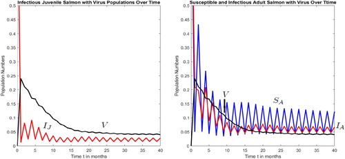However, as β increases past $\text{β}\approx 36$ and ${\mathcal{R}}_0>1$, the positive fixed point attractor undergoes an ISAv forced period-doubling bifurcation and the disease invades the juvenile and adult populations via a period 2 population cycle, where the juvenile-adult disease-free dynamics is a LAS fixed point attractor (see Figure 5). Figures 6 shows a LAS endemic period 2 population cycle in Model (6(6) $\left.\begin{array}{rl}{S}_{t+1}^J& =g\left(S_t^A\right)+{\hat{d}}_J\hat{m}{S}_t^J\left({\theta }_{1J}{\varphi }_J\left(I_t^J\right)+{\theta }_{2J}{\varphi }_J\left(I_t^A\right)+{\theta }_{3J}{\varphi }_V\left(V_t\right)\right)\\ I_{t+1}^J& ={\hat{d}}_J\hat{m}{S}_t^J{\hat{\mathrm{\Phi }}}_J\left(I_t^J,I_t^A,V_t\right)+{\hat{d}}_J\hat{m}{\hat{\mu }}_J{I}_t^J\\ S_{t+1}^A& ={\hat{d}}_A\left(m{S}_t^J+S_t^A\right)\left({\theta }_{1A}{\varphi }_A\left(I_t^J\right)+{\theta }_{2A}{\varphi }_A\left(I_t^A\right)+{\theta }_{3A}{\varphi }_V\left(V_t\right)\right)\\ I_{t+1}^A& ={\hat{d}}_A\left(m{S}_t^J+S_t^A\right){\hat{\mathrm{\Phi }}}_A\left(I_t^J,I_t^A,V_t\right)+{\hat{d}}_A{\hat{\mu }}_A\left(m{I}_t^J+I_t^A\right)\\ V_{t+1}& ={\hat{d}}_V\left(V_t+{\delta }_J{I}_t^J+{\delta }_A{I}_t^A\right)\end{array}\right\}$(6) ), where $\text{β}=49$ and all the other parameter values are fixed at their current values in Figure 5. That is, in age-structured ISAv models, the period of the juvenile-adult disease-free susceptible salmon population cycle does not in general determine the period of the juvenile-adult infectious salmon population cycles. This determination depends on the model recruitment function and parameter values. In Figures 5 and 6 for illustration, the numerical value chosen for the fraction of juvenile salmon that die from ISAv per unit time, ${\mu }_J=0.7$, is much greater than the value chosen for the fraction of the adult salmon that die from the disease, ${\mu }_A=0.001$. Consequently, in Figures 5 and 6, the number of ISA infectious juvenile salmon is less than the number of infectious adult salmon.

Figure 5. With initial population numbers, $(S_0^J,I_0^J,S_0^A,I_0^A,V_0)=(100,10,100,10,5)$, the disease-free equilibrium dynamics drives the ISAv disease equilibrium dynamics and the disease invades both the juvenile and adult populations via a fixed point attractor when ${\text{β}}_J={\text{β}}_A={\eta }_J={\eta }_A=\text{β}$ $\in (6.218,36)$, ${\text{β}}_V=0.01$ and ${\mathcal{R}}_0>1$. As β increases past β $\approx 36$ and ${\mathcal{R}}_0>1$, the positive fixed point undergoes an ISAv forced period-doubling bifurcation and the disease invades the juvenile and adult populations via a period 2 population cycle, where $r=e^4\approx 54.598$, $b=1,d_J=0.98,$ $d_A=0.9$, $d_V=0.2$, m = 0.3, ${\theta }_{1J}={\theta }_{1A}=0.6$, ${\theta }_{2J}={\theta }_{2A}=0.01$, ${\theta }_{3J}={\theta }_{3A}=0.39,$ ${\mu }_J=0.7$, ${\mu }_A=0.001,$ ${\delta }_J=0.2$ and ${\delta }_A=0.1$.

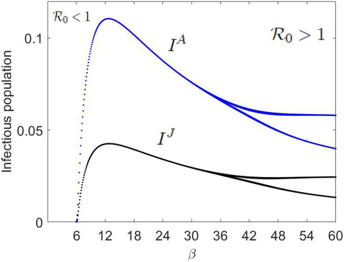
Figure 6. The disease-free fixed point population dynamics does not drive the ISAv disease dynamics and the disease invades both juvenile and adult populations via a period 2 population cycle, where ${\eta }_J={\eta }_A={\text{β}}_J={\text{β}}_A=\text{β}=49$ and all the other parameter values as in Figure 5.

4. Concluding remarks

We use juvenile-adult SIR and ISAv discrete-time infectious disease models with intrinsically generated demographic population cycles, extensions of unstructured models in [35], to explore the effects of age structure on the persistence or extinction of disease infection and the basic reproduction number, ${\mathcal{R}}_0$. Unlike the one-dimensional disease-free system in [35], our juvenile-adult disease-free system, Model (2(2) $\left.\begin{array}{rl}{S}_{t+1}^J& =g\left(S_t^A\right)+\left(1-d_J\right)\left(1-m\right)S_t^J\\ S_{t+1}^A& =\left(1-d_A\right)\left(m{S}_t^J+S_t^A\right)\end{array}\right\}$(2) ), is a system of two equations. Model (2(2) $\left.\begin{array}{rl}{S}_{t+1}^J& =g\left(S_t^A\right)+\left(1-d_J\right)\left(1-m\right)S_t^J\\ S_{t+1}^A& =\left(1-d_A\right)\left(m{S}_t^J+S_t^A\right)\end{array}\right\}$(2) ) exhibits only equilibrium dynamics when the recruitment function is the Beverton-Holt model. However, when the recruitment function is the Ricker model, Model (2(2) $\left.\begin{array}{rl}{S}_{t+1}^J& =g\left(S_t^A\right)+\left(1-d_J\right)\left(1-m\right)S_t^J\\ S_{t+1}^A& =\left(1-d_A\right)\left(m{S}_t^J+S_t^A\right)\end{array}\right\}$(2) ) exhibits a range of dynamic behaviours from stable equilibrium to deterministic period k population cycles to Neimark-Sacker bifurcations and deterministic chaos, where $k\ge 1$. When ${\mathcal{R}}_0<1$ and the juvenile-adult demographic equation (in the absence of the disease) has a locally asymptotically stable period k population cycle, we prove the local asymptotic stability of the juvenile-adult disease-free period k cycle. That is, the disease dies out in the juvenile and adult populations whenever ${\mathcal{R}}_0<1$. Also, under the same period k juvenile-adult demographic assumption, we prove that the juvenile-adult disease-free period k population cycle is unstable and the disease invades the juvenile and adult populations when ${\mathcal{R}}_0>1$.

When ${\mathcal{R}}_0>1$, in the SIR model, our simulations show that the period of the juvenile-adult demographic disease-free period k population cycle is the same as the period of the juvenile-adult SIR infectious population cycle. That is, the juvenile-adult demographic dynamics drives the juvenile-adult SIR disease dynamics. In stark contrast, when ${\mathcal{R}}_0>1$ we illustrate in Figures 5 and 6 that the juvenile-adult demographic dynamics does not in general drive the juvenile-adult ISAv disease dynamics. These simulation results are in agreement with that of the unstructured models in [35]. That is, the period of demographic population cycles do not determine the period of ISAv infectious populations, but do appear to predict the period of SIR infectious populations.

Acknowledgments

We thank the two anonymous reviewers for a thorough reading and helpful comments that improved our exposition.

Disclosure statement

No potential conflict of interest was reported by the author(s).

Additional information

Funding

A.-A.Y. was partially supported by DHS Center Of Excellence for Command, Control and Interoperability at Rutgers University, NSF Computational Sustainability Grant # CCF – 1522054, and NSF Award # DMS-1743144.

References

- L. Allen, Some discrete-time SI, SIR and SIS epidemic models, Math. Biosci. 124 (1994), pp. 83–105. doi: 10.1016/0025-5564(94)90025-6
- L. Allen and P. van den Driessche, The basic reproduction number in some discrete-time epidemic models, J. Difference Equations Appl. 14(10–11) (2008), pp. 1127–1147. doi: 10.1080/10236190802332308
- R. Beverton, S. Holt, On the Dynamics of Exploited Fish Populations, Fishery Investigations, Series II, Marine Fisheries, 19 [1-533], Her Majesty's Stationary Office, London, 1957.
- O.N. Bjørnstad, R.M. Nisbet, and J.M. Fromentin, Trends and cohort resonant effects in age-structured populations, J. Anim. Ecol. 73(6) (2004), pp. 1157–1167. doi: 10.1111/j.0021-8790.2004.00888.x
- L.W. Botsford and D.E. Wickham, Behavior of age-specific, density-dependent models and the Northern California dungeness crab fishery, J. Fish. Res. Board Can. 35 (1978), pp. 833–843. doi: 10.1139/f78-134
- L.W. Botsford, M.D. Holland, J.F. Samhouri, J.W. White, and A. Hastings, Importance of age structure in models of the response of upper trophic levels to fishing and climate change, ICES J. Mar. Sci. 68(6) (2011), pp. 1270–1283. doi: 10.1093/icesjms/fsr042
- F. Brauer, Z. Feng, and C. Castillo-Chavez, Discrete epidemic models, Math. Biosci. Eng. 7 (2010), pp. 1–15. doi: 10.3934/mbe.2010.7.1
- C. Castillo-Chavez and A.-A. Yakubu, Dispersal, disease and life-history evolution, Math. Biosci. 173 (2001), pp. 35–53. doi: 10.1016/S0025-5564(01)00065-7
- H. Caswell, Matrix Population Models: Construction, Analysis, and Interpretation, Sinauer, Sunderland, MA, 2001.
- J.M. Cushing, An Introduction to Structured Population Dynamics, Conference Series in Applied Mathematics, vol. 71, SIAM, Philadelphia, 1998.
- J.M. Cushing and O. Diekmann, The many guises of R0 (a diadactic note), J. Theor. Biol. 404 (2016), pp. 295–302. doi: 10.1016/j.jtbi.2016.06.017
- M. Devold, B. Krossay, V. Aspehaug, and A. Nylund, Use of RT-PCR for diagnosis of infectious salmon anaemia virus (ISAv) in carrier sea trout Salmo trutta after experimental infection, Dis. Aquat. Organ. 40 (2000), pp. 9–18. doi: 10.3354/dao040009
- O. Diekmann, J.A.P. Heesterbeek, and J.A.J. Metz, On the definition and computation of the basic reproduction ratio R0 in models for infectious diseases in heterogeneous populations, J. Math. Biol. 28 (1990), pp. 365–382. doi: 10.1007/BF00178324
- S. Elaydi, Discrete Chaos, Second Edition: With Applications in Science and Engineering, 2nd ed., Chapman & Hall/CRC, Boca Raton, 1999.
- J. Franke and A.-A. Yakubu, Principles of competitive exclusion for discrete populations with reproducing juveniles and adults, Nonlinear Anal. Theory Methods Appl. 30 (1997), pp. 1197–1205. doi: 10.1016/S0362-546X(97)00299-X
- J. Franke and A.-A. Yakubu, Attenuant cycles in periodically forced discrete-time age structured population models, J. Math. Anal. Appl. 316 (2006), pp. 69–86. doi: 10.1016/j.jmaa.2005.04.061
- J. Franke and A.-A. Yakubu, Globally attracting attenuant versus resonant cycles in compensatory Leslie models, Math. Biosci. 204 (2006), pp. 1–20. doi: 10.1016/j.mbs.2006.08.016
- J. Guckenheimer, G. Oster, and A. Ipaktchi, The dynamics of density dependent population models, J. Math. Biol. 4 (1978), pp. 101–147. doi: 10.1007/BF00275980
- F.S.B. Kibenge, O.N. Garate, G.R. Johnson, R. Arriagada, M.J.T. Kibenge, and D. Wadowska, Isolation and identification of infectious salmon anaemia virus (ISAv) from Coho salmon in Chile, Dis. Aquat. Organ. 45(1) (2001), pp. 9–18. doi: 10.3354/dao045009
- M. Krkosek, M.A. Lewis, and J.P. Volpe, Transmission dynamics of parasitic sea lice from farm to wild salmon, Proc. R. Soc. B. 272 (2005), pp. 689–696. doi: 10.1098/rspb.2004.3027
- J.P. La Salle, The Stability of Dynamical Systems, SIAM, Philadelphia, 1976.
- S.A. Levin and C.P. Goodyear, Analysis of an age-structured fishery model, J. Math. Biol. 9 (1980), pp. 245–274. doi: 10.1007/BF00276028
- D.A. Levy and C.C. Wood, Review of proposed mechanisms for sockeye salmon population cycles in the Fraser river, Bull. Math. Biol. 54(2–3) (1992), pp. 241–261. doi: 10.1016/S0092-8240(05)80025-4
- N. Li and A.-A. Yakubu, A Juvenile-Adult discrete-time production model of exploited fishery systems, Nat. Resource Modeling 25(2) (2012), pp. 273–324. doi: 10.1111/j.1939-7445.2011.00107.x
- S.H. Marshall, R. Ramírez, A. Labra, M. Carmona, and C. Muñoz, Bona fide evidence for natural vertical transmission of infectious salmon anemia virus in freshwater brood stocks of farmed salmon (Salmo salar) in Chile, J. Virol. 88(11) (2014), pp. 6012–6018. doi: 10.1128/JVI.03670-13
- R.M. May, Simple mathematical models with very complicated dynamics, Nature 261 (1976), pp. 459–467. doi: 10.1038/261459a0
- K.J. Melville and S.G. Griffiths, Absence of vertical transmission of infectious salmon anemia virus (ISAV) from individually infected Atlantic salmon Salmo salar, Dis. Aquat. Organ. 38(3) (1999), pp. 231–234. doi: 10.3354/dao038231
- E. Milliken and S.S. Pilyugim, A model of infectious salmon anemia virus with viral diffusion between wild and farmed patches, Discrete Cont. Dyn. Sys. B 21(6) (2016), pp. 1869–1893. doi: 10.3934/dcdsb.2016027
- R.A. Myers, G. Mertz, J.M. Bridson, and M.J. Bradford, Simple dynamics underlie sockeye salmon (Oncorhynchus nerka) cycles, Canad. J. Fish. Aquat. Sci. 55 (1998), pp. 2355–2364. doi: 10.1139/f98-059
- G.F. Oster, The dynamics of nonlinear models with age structure, in Studies in Mathematical Biology II: Populations and Communities, S.A. Levin, ed., Mathematical Association of America, Washington, D.C., 1978, pp. 411–438.
- W.E. Ricker, Stock and recruitment, J. Fish. Res. Board Can. 11 (1954), pp. 559–623. doi: 10.1139/f54-039
- W.E. Ricker, The historical development, in Fish Population Dynamics, L. A. Gulland, ed., Wiley, London, 1975, pp. 1–26.
- H.L. Smith, Cooperative systems of differential equations with concave nonlinearities, Nonlinear Anal. Theory Methods Appl. 10(10) (1986), pp. 1037–1052. doi: 10.1016/0362-546X(86)90087-8
- P. van den Driessche, Reproduction numbers of infectious disease models, Infect. Dis. Model. 2 (2017), pp. 1–16.
- P. van den Driessche and A.-A. Yakubu, Demographic population cycles and R0 in discrete-time epidemic models, J. Biol. Dyn. 12(1) (2018), pp. 961–986. DOI: 10.1080/17513758.2018.1537449. doi: 10.1080/17513758.2018.1541104
- P. van den Driessche and A.-A. Yakubu, Disease extinction versus persistence in discrete-time epidemic models, Bull. Math. Biol. (2018). DOI: 10.1007/s11538-018-0426-2.
- A. Veprauskas and J.M. Cushing, A juvenile-adult population model: Climate change, cannibalism, reproductive synchrony, and strong Allee effects, J. Biol. Dynam. 11(Sup1) (2017), pp. 1–24. doi: 10.1080/17513758.2015.1131853
- H.I. Wergeland and R.A. Jakobsen, A salmonid cell line (TO) for production of infectious salmon anaemia virus (ISAv), Dis. Aquat. Organ. 44 (2001), pp. 183–190. doi: 10.3354/dao044183
- A.-A. Yakubu, Introduction to discrete-time epidemic models, DIMACS Ser. Discrete Math. Theor. Comput. Sci. 75 (2010), pp. 83–109. doi: 10.1090/dimacs/075/04