Stability and bifurcation analysis of an HIV-1 infection model with a general incidence and CTL immune response

Abstract

In this paper, with eclipse stage in consideration, we propose an HIV-1 infection model with a general incidence rate and CTL immune response. We first study the existence and local stability of equilibria, which is characterized by the basic infection reproduction number ${\mathcal{R}}_0$ and the basic immunity reproduction number ${\mathcal{R}}_1$. The local stability analysis indicates the occurrence of transcritical bifurcations of equilibria. We confirm the bifurcations at the disease-free equilibrium and the infected immune-free equilibrium with transmission rate and the decay rate of CTLs as bifurcation parameters, respectively. Then we apply the approach of Lyapunov functions to establish the global stability of the equilibria, which is determined by the two basic reproduction numbers. These theoretical results are supported with numerical simulations. Moreover, we also identify the high sensitivity parameters by carrying out the sensitivity analysis of the two basic reproduction numbers to the model parameters.

Keywords:

• HIV infection
• incidence
• Lyapunov function
• global stability
• bifurcation

1. Introduction

HIV (Human Immunodeficiency Virus) is the pathogen causing AIDS (Acquired ImmunoDeficiency Syndrome). Now, HIV has been a major global public health issue. There were approximately 37.9 million people living with HIV at the end of 2018 with 1.7 million people becoming newly infected in 2018 globally [34]. Though an estimated entry into the human population in the early twentieth century [9], HIV was identified as responsible for AIDS only until 1984 [10]. Since then, HIV infection has been intensively studied and massive drug development efforts have been made. “Yet despite these advances, we still do not have a clear explanation for the pathogenesis of infection nor therapies that can permanently cure the infection” [12]. Mathematical models have played an important role in enhancing understanding of HIV infection dynamics and helping generating ideas on how to treat the infection. Here we only focus on within-host HIV models. We refer to [25] for a recent review for such models.

In the pioneering work [22], Nowak and Bangham proposed some simple models to explore the relation between antiviral immune responses, virus load, and virus diversity. Since then, these models have been modified to reflect the effects of many other factors such as delay, eclipse phase, treatment, drug resistance, nonlinear incidence, transmission modes, multi-strain of viruses, co-infection, super-infection, vaccination, age/stage structure, spatial heterogeneity, and so on. We refer to [1–3, 8, 14, 15, 17, 19–21, 23, 24, 28, 29, 32] as samples of works in the last five years to indicate how active the study on HIV-1 infection still is.

In particular, the HIV eclipse phase is the time period from a virus entering a target cell to the infected cell becoming infectious and producing new viruses. Of the four phases of HIV infection (acute, eclipse, chronic, and AIDS), the first three are currently the window of opportunity for viral clearance. There are many ways to describe the eclipse phase, which include delay models and age-structured models (see, for example, the references in [26]). In [26], Rong and his coworkers introduced a stage-structured HIV-1 infection model. Their model is described by the following system of four ordinary differential equations, (1) $\{\begin{array}{l}{\displaystyle \dot{x}(t)=\lambda -\mu x(t)-\beta x(t)v(t)+\delta w(t),}\\ {\displaystyle \dot{w}(t)=\beta x(t)v(t)-(\delta +\eta +q)w(t),}\\ {\displaystyle \dot{y}(t)=qw(t)-\alpha y(t),}\\ {\displaystyle \dot{v}(t)=\sigma y(t)-\gamma v(t),}\end{array}$(1) where $x(t)$, $w(t)$, $y(t)$, and $v(t)$ represent the concentrations of uninfected CD4${}^{+}$ T cells, infected cells in the eclipse stage, productively infected cells, and free viruses at time t, respectively. One feature of model (1(1) $\{\begin{array}{l}{\displaystyle \dot{x}(t)=\lambda -\mu x(t)-\beta x(t)v(t)+\delta w(t),}\\ {\displaystyle \dot{w}(t)=\beta x(t)v(t)-(\delta +\eta +q)w(t),}\\ {\displaystyle \dot{y}(t)=qw(t)-\alpha y(t),}\\ {\displaystyle \dot{v}(t)=\sigma y(t)-\gamma v(t),}\end{array}$(1) ) is that a portion of infected cells in the eclipse phase may revert to the uninfected cells. The biological meanings of the parameters are summarized in Table 1.

Table 1. The biological meanings of the parameters in model (1(1) $\{\begin{array}{l}{\displaystyle \dot{x}(t)=\lambda -\mu x(t)-\beta x(t)v(t)+\delta w(t),}\\ {\displaystyle \dot{w}(t)=\beta x(t)v(t)-(\delta +\eta +q)w(t),}\\ {\displaystyle \dot{y}(t)=qw(t)-\alpha y(t),}\\ {\displaystyle \dot{v}(t)=\sigma y(t)-\gamma v(t),}\end{array}$(1) ).

Parameter	Biological meaning
λ	recruitment rate of uninfected CD4${}^{+}$ T cells
μ	natural death rate of CD4${}^{+}$ T cells
β	infection rate
δ	rate at which infected cells in the eclipse phase reverting to the uninfected class
η	death rate of infected cells in the eclipse phase
q	rate of infected cells in the eclipse phase becoming productively infected cells
α	death rate of productively infected cells
σ	production rate of virions by an infected cell
γ	clearance rate of free viruses

Rong et al. analysed the local stability of the infected equilibrium of (1(1) $\{\begin{array}{l}{\displaystyle \dot{x}(t)=\lambda -\mu x(t)-\beta x(t)v(t)+\delta w(t),}\\ {\displaystyle \dot{w}(t)=\beta x(t)v(t)-(\delta +\eta +q)w(t),}\\ {\displaystyle \dot{y}(t)=qw(t)-\alpha y(t),}\\ {\displaystyle \dot{v}(t)=\sigma y(t)-\gamma v(t),}\end{array}$(1) ). Later on, Buonomo and Vargas-De-Léon [4] provided some sufficient conditions on its global stability by using the Lyapunov direct method and a geometric method based on compounded matrices.

On the one hand, the incidence in (1(1) $\{\begin{array}{l}{\displaystyle \dot{x}(t)=\lambda -\mu x(t)-\beta x(t)v(t)+\delta w(t),}\\ {\displaystyle \dot{w}(t)=\beta x(t)v(t)-(\delta +\eta +q)w(t),}\\ {\displaystyle \dot{y}(t)=qw(t)-\alpha y(t),}\\ {\displaystyle \dot{v}(t)=\sigma y(t)-\gamma v(t),}\end{array}$(1) ) is the bilinear one. However, experiments [7] have strongly suggested that the incidence is an increasing function of the parasite dose, and is usually sigmoidal in shape (see, for example, [30]). As a result, Hesaaraki and Sabzevari [11] modified (1(1) $\{\begin{array}{l}{\displaystyle \dot{x}(t)=\lambda -\mu x(t)-\beta x(t)v(t)+\delta w(t),}\\ {\displaystyle \dot{w}(t)=\beta x(t)v(t)-(\delta +\eta +q)w(t),}\\ {\displaystyle \dot{y}(t)=qw(t)-\alpha y(t),}\\ {\displaystyle \dot{v}(t)=\sigma y(t)-\gamma v(t),}\end{array}$(1) ) by replacing $\beta xv$ with $\frac{\beta xv}{1+av}$. Using the same approaches of Buonomo and Vargas-De-Léon [4], they obtained sufficient conditions on the global stability of the equilibria of the resulting system. On the other hand, in most virus infections, cytotoxic T lymphocytes (CTLs) play a critical role in antiviral defence by attacking the productively infected cells. In [18], Lv et al. modified (1(1) $\{\begin{array}{l}{\displaystyle \dot{x}(t)=\lambda -\mu x(t)-\beta x(t)v(t)+\delta w(t),}\\ {\displaystyle \dot{w}(t)=\beta x(t)v(t)-(\delta +\eta +q)w(t),}\\ {\displaystyle \dot{y}(t)=qw(t)-\alpha y(t),}\\ {\displaystyle \dot{v}(t)=\sigma y(t)-\gamma v(t),}\end{array}$(1) ) to study the following system with Beddington-DeAngelis incidence and CTL immune response, (2) $\{\begin{array}{l}{\displaystyle \dot{x}=\lambda -\mu x-\frac{\beta xv}{1+mx+nv}+\delta w,}\\ {\displaystyle \dot{w}=\frac{\beta xv}{1+mx+nv}-(\delta +\eta +q)w,}\\ {\displaystyle \dot{y}=qw-\alpha y-pyz,}\\ {\displaystyle \dot{v}=\sigma y-\gamma v,}\\ {\displaystyle \dot{z}=kyz-cz.}\end{array}$(2) Here z is the concentration of CTLs; p is the rate of productively infected cells removed by CTLs; k is the number of virions produced by a productively infected cell; c is the decay rate of CTLs; and the meanings of the other parameters are the same as those in Table 1. With the Lyapunov direct method, established are conditions on the global stability of equilibria in terms of the basic reproduction number and the immune response reproduction number. Later on, Maziane et al. [20] considered a variation of (2(2) $\{\begin{array}{l}{\displaystyle \dot{x}=\lambda -\mu x-\frac{\beta xv}{1+mx+nv}+\delta w,}\\ {\displaystyle \dot{w}=\frac{\beta xv}{1+mx+nv}-(\delta +\eta +q)w,}\\ {\displaystyle \dot{y}=qw-\alpha y-pyz,}\\ {\displaystyle \dot{v}=\sigma y-\gamma v,}\\ {\displaystyle \dot{z}=kyz-cz.}\end{array}$(2) ) by replacing $\frac{\beta xv}{1+mx+nv}$ with $\frac{\beta xv}{1+{\alpha }_{1}x+{\alpha }_{2}v+{\alpha }_{3}xv}$ and similar results were derived.

Motivated by the above discussion, in this paper, we investigate the following HIV-1 infection model with eclipse phase and CTL immune response, (3) $\{\begin{array}{l}{\displaystyle \dot{x}(t)=\lambda -\mu x(t)-x(t)f(v(t))+\delta w(t),}\\ {\displaystyle \dot{w}(t)=x(t)f(v(t))-(\delta +\eta +q)w(t),}\\ {\displaystyle \dot{y}(t)=qw(t)-\alpha y(t)-py(t)z(t),}\\ {\displaystyle \dot{v}(t)=\sigma y(t)-\gamma v(t),}\\ {\displaystyle \dot{z}(t)=ky(t)z(t)-cz(t).}\end{array}$(3) Here the meanings of the parameters are the same as before. The function f in the nonlinear incidence $xf(v)$ is continuously differentiable on ${\mathbb{R}}_{+}$ and satisfies

1. $f(0)=0$;

2. $f^{\prime }(v)>0$ for $v\ge 0$;

3. f is concave down on ${\mathbb{R}}_{+}$.

Biologically, assumptions (H1)–(H3) mean that the disease transmission rate is monotonically increasing, but subject to saturation effects. Note that (H1) and (H2) combined imply that $f(v)>0$ for v>0. It is clear that incidence functions such as the bilinear incidence with $f(v)=\beta v$ and the Holling-type II incidence with $f(v)=\frac{\beta v}{1+\alpha v}$ satisfy (H1)–(H3).

The main results of this paper are about the global stability of equilibria of (3(3) $\{\begin{array}{l}{\displaystyle \dot{x}(t)=\lambda -\mu x(t)-x(t)f(v(t))+\delta w(t),}\\ {\displaystyle \dot{w}(t)=x(t)f(v(t))-(\delta +\eta +q)w(t),}\\ {\displaystyle \dot{y}(t)=qw(t)-\alpha y(t)-py(t)z(t),}\\ {\displaystyle \dot{v}(t)=\sigma y(t)-\gamma v(t),}\\ {\displaystyle \dot{z}(t)=ky(t)z(t)-cz(t).}\end{array}$(3) ). The paper is organized as follows. In Section 2, we give some preliminary results of (3(3) $\{\begin{array}{l}{\displaystyle \dot{x}(t)=\lambda -\mu x(t)-x(t)f(v(t))+\delta w(t),}\\ {\displaystyle \dot{w}(t)=x(t)f(v(t))-(\delta +\eta +q)w(t),}\\ {\displaystyle \dot{y}(t)=qw(t)-\alpha y(t)-py(t)z(t),}\\ {\displaystyle \dot{v}(t)=\sigma y(t)-\gamma v(t),}\\ {\displaystyle \dot{z}(t)=ky(t)z(t)-cz(t).}\end{array}$(3) ), which include the boundedness of solutions and the existence of equilibria. The existence of equilibria is characterized by two basic reproduction numbers. Then we discuss the local stability of equilibria. It turns out that transcritical bifurcations of equilibria occur. We confirm them with the transmission rate and decay rate of CTLs as bifurcation parameters. After that, we employ the Lyapunov direction method to establish the global stability of the equilibria. Finally, we illustrate these theoretical results with numerical simulations and carry out the sensitivity analysis of the two basic reproduction numbers to the parameters. The paper ends with a brief summary and discussion.

2. Preliminaries

The initial conditions for system (3(3) $\{\begin{array}{l}{\displaystyle \dot{x}(t)=\lambda -\mu x(t)-x(t)f(v(t))+\delta w(t),}\\ {\displaystyle \dot{w}(t)=x(t)f(v(t))-(\delta +\eta +q)w(t),}\\ {\displaystyle \dot{y}(t)=qw(t)-\alpha y(t)-py(t)z(t),}\\ {\displaystyle \dot{v}(t)=\sigma y(t)-\gamma v(t),}\\ {\displaystyle \dot{z}(t)=ky(t)z(t)-cz(t).}\end{array}$(3) ) are (4) $x(0\ge 0,w(0)\ge 0,y(0)\ge 0,v(0)\ge 0,z(0)\ge 0.$(4) With standard arguments, one can easily see that (3(3) $\{\begin{array}{l}{\displaystyle \dot{x}(t)=\lambda -\mu x(t)-x(t)f(v(t))+\delta w(t),}\\ {\displaystyle \dot{w}(t)=x(t)f(v(t))-(\delta +\eta +q)w(t),}\\ {\displaystyle \dot{y}(t)=qw(t)-\alpha y(t)-py(t)z(t),}\\ {\displaystyle \dot{v}(t)=\sigma y(t)-\gamma v(t),}\\ {\displaystyle \dot{z}(t)=ky(t)z(t)-cz(t).}\end{array}$(3) ) with the initial condition (4(4) $x(0\ge 0,w(0)\ge 0,y(0)\ge 0,v(0)\ge 0,z(0)\ge 0.$(4) ) has a unique solution $(x(t),w(t),y(t),v(t),z(t))$ on ${\mathbb{R}}_{+}$. Moreover, the solution stays nonnegative on ${\mathbb{R}}_{+}$.

For any solution of (3(3) $\{\begin{array}{l}{\displaystyle \dot{x}(t)=\lambda -\mu x(t)-x(t)f(v(t))+\delta w(t),}\\ {\displaystyle \dot{w}(t)=x(t)f(v(t))-(\delta +\eta +q)w(t),}\\ {\displaystyle \dot{y}(t)=qw(t)-\alpha y(t)-py(t)z(t),}\\ {\displaystyle \dot{v}(t)=\sigma y(t)-\gamma v(t),}\\ {\displaystyle \dot{z}(t)=ky(t)z(t)-cz(t).}\end{array}$(3) ), we have $\begin{array}{rl}\dot{x}+\dot{w}+\dot{y}+\frac{p}{k}\dot{z}& =\lambda -\mu x-\eta w-\alpha y-\frac{pc}{k}z\\ & \le \lambda -b(x+w+y+\frac{p}{k}z),\end{array}$where $b=min\{c,\alpha ,\eta ,\mu \}$. It follows that (5) $\underset{t\to \mathrm{\infty }}{lim sup}(x+w+y+\frac{p}{k}z)\le \frac{\lambda }{b}$(5) and if $x(t_0)+w(t_0)+y(t_0)+\frac{p}{k}z(t_0)\le \frac{\lambda }{b}$ for some $t_0\in {\mathbb{R}}_{+}$ then $x(t)+w(t)+y(t)+\frac{p}{k}z(t)\le \frac{\lambda }{b}$ for all $t\ge t_0$. The fourth equation of system (3(3) $\{\begin{array}{l}{\displaystyle \dot{x}(t)=\lambda -\mu x(t)-x(t)f(v(t))+\delta w(t),}\\ {\displaystyle \dot{w}(t)=x(t)f(v(t))-(\delta +\eta +q)w(t),}\\ {\displaystyle \dot{y}(t)=qw(t)-\alpha y(t)-py(t)z(t),}\\ {\displaystyle \dot{v}(t)=\sigma y(t)-\gamma v(t),}\\ {\displaystyle \dot{z}(t)=ky(t)z(t)-cz(t).}\end{array}$(3) ) together with (5(5) $\underset{t\to \mathrm{\infty }}{lim sup}(x+w+y+\frac{p}{k}z)\le \frac{\lambda }{b}$(5) ) implies that $\underset{t\to \mathrm{\infty }}{lim sup}v\le \frac{\lambda \sigma }{b\gamma }.$

Proposition 2.1

The set Γ defined by $\mathrm{\Gamma }=\{(x,w,y,v,z)\in {\mathbb{R}}_{+}^5:x+w+y+\frac{p}{k}z\le \frac{\lambda }{b},v\le \frac{\lambda \sigma }{b\gamma }\}$is an attracting and positively invariant set of (3(3) $\{\begin{array}{l}{\displaystyle \dot{x}(t)=\lambda -\mu x(t)-x(t)f(v(t))+\delta w(t),}\\ {\displaystyle \dot{w}(t)=x(t)f(v(t))-(\delta +\eta +q)w(t),}\\ {\displaystyle \dot{y}(t)=qw(t)-\alpha y(t)-py(t)z(t),}\\ {\displaystyle \dot{v}(t)=\sigma y(t)-\gamma v(t),}\\ {\displaystyle \dot{z}(t)=ky(t)z(t)-cz(t).}\end{array}$(3) ).

Proof.

The discussion before the statement of Proposition 2.1 tells us that Γ attracts every solution of (3(3) $\{\begin{array}{l}{\displaystyle \dot{x}(t)=\lambda -\mu x(t)-x(t)f(v(t))+\delta w(t),}\\ {\displaystyle \dot{w}(t)=x(t)f(v(t))-(\delta +\eta +q)w(t),}\\ {\displaystyle \dot{y}(t)=qw(t)-\alpha y(t)-py(t)z(t),}\\ {\displaystyle \dot{v}(t)=\sigma y(t)-\gamma v(t),}\\ {\displaystyle \dot{z}(t)=ky(t)z(t)-cz(t).}\end{array}$(3) ). Now, let $(x(0),w(0),y(0),v(0),z(0))\in \mathrm{\Gamma }$. Then $x(t)+w(t)+y(t)+\frac{p}{k}z(t)\le \frac{\lambda }{b}$ for every $t\in {\mathbb{R}}_{+}$ as mentioned before. We claim that $v(t)\le \frac{\lambda \sigma }{b\gamma }$ for $t\in {\mathbb{R}}_{+}$. If this is not true, then there exists $t_0\in {\mathbb{R}}_{+}$ such that $v(t_0)>\frac{\lambda \sigma }{b\gamma }$. Let $t_1=inf\{s\le t_0:v(t)>\frac{\lambda \sigma }{b\gamma }on[s,t_0]\}$. It follows that $v(t_1)=\frac{\lambda \sigma }{b\gamma }$. Obviously, there exists $t_2\in (t_1,t_0)$ such that $\dot{v}(t_2)>0$. However, $\dot{v}(t_2)=\sigma y(t_2)-\gamma v(t_2)<\sigma \frac{\lambda }{b}-\gamma \frac{\lambda \sigma }{b\gamma }=0,$a contradiction. This proves the claim and hence Γ is positively invariant.

Now, we consider the existence of equilibria of (3(3) $\{\begin{array}{l}{\displaystyle \dot{x}(t)=\lambda -\mu x(t)-x(t)f(v(t))+\delta w(t),}\\ {\displaystyle \dot{w}(t)=x(t)f(v(t))-(\delta +\eta +q)w(t),}\\ {\displaystyle \dot{y}(t)=qw(t)-\alpha y(t)-py(t)z(t),}\\ {\displaystyle \dot{v}(t)=\sigma y(t)-\gamma v(t),}\\ {\displaystyle \dot{z}(t)=ky(t)z(t)-cz(t).}\end{array}$(3) ).

System (3(3) $\{\begin{array}{l}{\displaystyle \dot{x}(t)=\lambda -\mu x(t)-x(t)f(v(t))+\delta w(t),}\\ {\displaystyle \dot{w}(t)=x(t)f(v(t))-(\delta +\eta +q)w(t),}\\ {\displaystyle \dot{y}(t)=qw(t)-\alpha y(t)-py(t)z(t),}\\ {\displaystyle \dot{v}(t)=\sigma y(t)-\gamma v(t),}\\ {\displaystyle \dot{z}(t)=ky(t)z(t)-cz(t).}\end{array}$(3) ) always has an infection-free equilibrium $E_0=(x_0,0,0,0,0)$, where $x_0=\frac{\lambda }{\mu }$. In fact, $E_0$ is the only infection-free equilibrium. Employing the next-generation matrix method in van den Driessche and Watmough [33], one can easily get the expression of the basic infection reproduction number ${\mathcal{R}}_0$ of system (3(3) $\{\begin{array}{l}{\displaystyle \dot{x}(t)=\lambda -\mu x(t)-x(t)f(v(t))+\delta w(t),}\\ {\displaystyle \dot{w}(t)=x(t)f(v(t))-(\delta +\eta +q)w(t),}\\ {\displaystyle \dot{y}(t)=qw(t)-\alpha y(t)-py(t)z(t),}\\ {\displaystyle \dot{v}(t)=\sigma y(t)-\gamma v(t),}\\ {\displaystyle \dot{z}(t)=ky(t)z(t)-cz(t).}\end{array}$(3) ), ${\mathcal{R}}_0=\frac{\lambda \sigma q}{\mu \alpha \gamma (\delta +\eta +q)}{f}^{\prime }(0).$An equilibrium of (3(3) $\{\begin{array}{l}{\displaystyle \dot{x}(t)=\lambda -\mu x(t)-x(t)f(v(t))+\delta w(t),}\\ {\displaystyle \dot{w}(t)=x(t)f(v(t))-(\delta +\eta +q)w(t),}\\ {\displaystyle \dot{y}(t)=qw(t)-\alpha y(t)-py(t)z(t),}\\ {\displaystyle \dot{v}(t)=\sigma y(t)-\gamma v(t),}\\ {\displaystyle \dot{z}(t)=ky(t)z(t)-cz(t).}\end{array}$(3) ) satisfies kyz−cz = 0 and hence either z = 0 or $y=\frac{c}{k}$.

We first consider the case where z = 0, which gives immune-free equilibria. At an immune-free equilibrium, we have (6a) $\begin{array}{rl}& \lambda -\mu x-xf(v)+\delta w=0,\end{array}$(6a) (6b) $\begin{array}{rl}& xf(v)-(\delta +\eta +q)w=0,\end{array}$(6b) (6c) $\begin{array}{rl}& qw-\alpha y=0,\end{array}$(6c) (6d) $\begin{array}{rl}& \sigma y-\gamma v=0.\end{array}$(6d) Adding (6a(6a) $\begin{array}{rl}& \lambda -\mu x-xf(v)+\delta w=0,\end{array}$(6a) ) and (6b(6b) $\begin{array}{rl}& xf(v)-(\delta +\eta +q)w=0,\end{array}$(6b) ) yields $x=\frac{\lambda -(\eta +q)w}{\mu },$which also implies that $w<\frac{\lambda }{\eta +q}$. Furthermore, it follows from (6c(6c) $\begin{array}{rl}& qw-\alpha y=0,\end{array}$(6c) ) and (6d(6d) $\begin{array}{rl}& \sigma y-\gamma v=0.\end{array}$(6d) ), respectively that $y=\frac{qw}{\alpha }\text{and}v=\frac{\sigma qw}{\alpha \gamma }.$Substituting the expressions of x and v above into (6b(6b) $\begin{array}{rl}& xf(v)-(\delta +\eta +q)w=0,\end{array}$(6b) ), we see that (7) $g(w)\triangleq \frac{\lambda -(\eta +q)w}{\mu }f\left(\frac{\sigma q}{\alpha \gamma }w\right)-(\delta +\eta +q)w=0.$(7) Clearly, $g(0)=0$, which gives the infection-free equilibrium $E_0$. In the following, we consider infected immune-free equilibria. Note that $g^{\prime }(0)=\frac{\lambda \sigma q}{\mu \alpha \gamma }{f}^{\prime }(0)-(\delta +\eta +q)=(\delta +\eta +q)({\mathcal{R}}_0-1).$If ${\mathcal{R}}_0>1$, then $g^{\prime }(0)>0$. This, combined with $g(0)=0$, implies that $g(w)>0$ for w>0 sufficiently small. Noting $g(\frac{\lambda }{\eta +q})=-\frac{\lambda (\delta +\eta +q)}{\eta +q}<0$, we see that g has at least one positive zero in $(0,\frac{\lambda }{\eta +q})$, which gives an infected immune-free equilibrium. Note that if $E_1=(x_1,w_1,y_1,v_1,0)$ is an infected immune-free equilibrium, then $\begin{array}{rl}{g}^{\prime }(w_1)& =-\frac{\eta +q}{\mu }f(v_1)+\frac{\sigma q}{\alpha \gamma }{x}_1{f}^{\prime }(v_1)-(\delta +\eta +q)\\ & =-\frac{\eta +q}{\mu }f(v_1)+\frac{\sigma q}{\alpha \gamma }{x}_1{f}^{\prime }(v_1)-\frac{\sigma q{x}_{1}f(v_1)}{\alpha \gamma v_1}\\ & =-\frac{\eta +q}{\mu }f(v_1)+\frac{\sigma q{x}_1}{\alpha \gamma v_1}(v_1{f}^{\prime }(v_1)-f(v_1))\\ & <0.\end{array}$To obtain the last inequality, we have used assumption (H3) that f is concave down. This fact immediately tells us that there can be at most one infected immune-free equilibrium and hence there is a unique infected immune-free equilibrium, denoted by $E_1=(x_1,w_1,y_1,v_1,0)$, when ${\mathcal{R}}_0>1$. Now assume that ${\mathcal{R}}_0\le 1$. Then $g^{\prime }(0)\le 0$. This, together with $g(0)=0$ and $g^{″}(0)=-\frac{\eta +q}{\mu }{f}^{\prime }(0)+\frac{\lambda (\sigma q{)}^2}{\mu (\alpha \gamma {)}^2}{f}^{″}(0)<0,$tells us that $g(w)<0$ for w>0 sufficiently small. We claim that g has no zero in $(0,\frac{\lambda }{\eta +q})$. Otherwise, at the first zero of g, the derivative of g is larger than or equal to zero, a contradiction to the fact that the derivative is less than zero. Therefore, if ${\mathcal{R}}_0\le 1$, then there is no infected immune-free equilibrium.

Next, we consider the case where $y=\frac{c}{k}$ and $z\ne 0$, that is, infected equilibria with immunity. In this case, an equilibrium satisfies (8a) $\begin{array}{rl}& \lambda -\mu x-xf(v)+\delta w=0,\end{array}$(8a) (8b) $\begin{array}{rl}& xf(v)-(\delta +\eta +q)w=0,\end{array}$(8b) (8c) $\begin{array}{rl}& qw-\frac{\alpha c}{k}-\frac{pc}{k}z=0,\end{array}$(8c) (8d) $\begin{array}{rl}& \frac{\sigma c}{k}-\gamma v=0.\end{array}$(8d) Clearly, (8d(8d) $\begin{array}{rl}& \frac{\sigma c}{k}-\gamma v=0.\end{array}$(8d) ) gives $v=\frac{\sigma c}{k\gamma }$, and as before $x=\frac{\lambda -(\eta +q)w}{\mu }$ from (8a(8a) $\begin{array}{rl}& \lambda -\mu x-xf(v)+\delta w=0,\end{array}$(8a) ) and (8b(8b) $\begin{array}{rl}& xf(v)-(\delta +\eta +q)w=0,\end{array}$(8b) ). Substituting both into (8b(8b) $\begin{array}{rl}& xf(v)-(\delta +\eta +q)w=0,\end{array}$(8b) ) yields (9) $w=\frac{\lambda f(\frac{\sigma c}{\gamma k})}{(\eta +q)f(\frac{\sigma c}{\gamma k})+\mu (\delta +\eta +q)}$(9) and hence $x=\frac{\lambda (\delta +\eta +q)}{(\eta +q)f(\frac{\sigma c}{\gamma k})+\mu (\delta +\eta +q)}$. From (9(9) $w=\frac{\lambda f(\frac{\sigma c}{\gamma k})}{(\eta +q)f(\frac{\sigma c}{\gamma k})+\mu (\delta +\eta +q)}$(9) ) and (8c(8c) $\begin{array}{rl}& qw-\frac{\alpha c}{k}-\frac{pc}{k}z=0,\end{array}$(8c) ), we see that there is an infected equilibrium with immunity (and if exists then there is a unique one) if and only if ${\mathcal{R}}_1>1$, where ${\mathcal{R}}_1=\frac{kq\lambda f\left(\frac{\sigma c}{\gamma k}\right)}{\alpha c[(\eta +q)f\left(\frac{\sigma c}{\gamma k}\right)+\mu (\delta +\eta +q)]}.$In this case, $z=\frac{\alpha }{p}({\mathcal{R}}_1-1)$. ${\mathcal{R}}_1$ is called the basic immunity reproduction number.

Note that ${\mathcal{R}}_1<{\mathcal{R}}_0$ as shown below. From the concavity of f, we know that $f(v)\le v{f}^{\prime }(0)$ for all $v\ge 0$. Thus $\begin{array}{rl}{\mathcal{R}}_1& =\frac{\lambda kqf(v)}{\mu \alpha c(\delta +\eta +q)+\alpha c(\eta +q)f(v)}\\ & \le \frac{\lambda kq{f}^{\prime }(0)v}{\mu \alpha c(\delta +\eta +q)+\alpha c(\eta +q)f(v)}\\ & <\frac{\lambda \sigma q{f}^{\prime }(0)}{\mu \alpha \gamma (\delta +\eta +q)}\\ & ={\mathcal{R}}_0.\end{array}$${\mathcal{R}}_1<{\mathcal{R}}_0$ implies that, for an infected equilibrium with immunity to exist, it is necessary that an infected immunity-free equilibrium exists. This agrees with the biological process. Actually, one can obtain ${\mathcal{R}}_1$ in the same manner as for ${\mathcal{R}}_0$ by the next generation matrix method at $E_1$.

In summary, we have shown the following result on the existence of equilibria.

Theorem 2.1

1. If ${\mathcal{R}}_0\le 1$, then (3(3) $\{\begin{array}{l}{\displaystyle \dot{x}(t)=\lambda -\mu x(t)-x(t)f(v(t))+\delta w(t),}\\ {\displaystyle \dot{w}(t)=x(t)f(v(t))-(\delta +\eta +q)w(t),}\\ {\displaystyle \dot{y}(t)=qw(t)-\alpha y(t)-py(t)z(t),}\\ {\displaystyle \dot{v}(t)=\sigma y(t)-\gamma v(t),}\\ {\displaystyle \dot{z}(t)=ky(t)z(t)-cz(t).}\end{array}$(3) ) only has the infection-free equilibrium $E_0$.

2. If ${\mathcal{R}}_1\le 1<{\mathcal{R}}_0$, then besides $E_0$, (3(3) $\{\begin{array}{l}{\displaystyle \dot{x}(t)=\lambda -\mu x(t)-x(t)f(v(t))+\delta w(t),}\\ {\displaystyle \dot{w}(t)=x(t)f(v(t))-(\delta +\eta +q)w(t),}\\ {\displaystyle \dot{y}(t)=qw(t)-\alpha y(t)-py(t)z(t),}\\ {\displaystyle \dot{v}(t)=\sigma y(t)-\gamma v(t),}\\ {\displaystyle \dot{z}(t)=ky(t)z(t)-cz(t).}\end{array}$(3) ) also has an infected immune-free equilibrium $E_1=(x_1,w_1,y_1,v_1,0)$, where $x_1=\frac{\lambda -(\eta +q)w_1}{\mu }$, $y_1=\frac{q{w}_1}{\alpha }$, $v_1=\frac{\sigma q{w}_1}{\alpha \gamma }$, and $w_1$ is the unique positive zero of g defined by (7(7) $g(w)\triangleq \frac{\lambda -(\eta +q)w}{\mu }f\left(\frac{\sigma q}{\alpha \gamma }w\right)-(\delta +\eta +q)w=0.$(7) ) in $(0,\frac{\lambda }{\eta +q})$.

3. If $1<{\mathcal{R}}_1(<{\mathcal{R}}_0)$, then in addition to $E_0$ and $E_1$, there is a unique infected equilibrium with immunity $E_2=(x_2,w_2,y_2,v_2,z_2)$ for (3(3) $\{\begin{array}{l}{\displaystyle \dot{x}(t)=\lambda -\mu x(t)-x(t)f(v(t))+\delta w(t),}\\ {\displaystyle \dot{w}(t)=x(t)f(v(t))-(\delta +\eta +q)w(t),}\\ {\displaystyle \dot{y}(t)=qw(t)-\alpha y(t)-py(t)z(t),}\\ {\displaystyle \dot{v}(t)=\sigma y(t)-\gamma v(t),}\\ {\displaystyle \dot{z}(t)=ky(t)z(t)-cz(t).}\end{array}$(3) ), where $x_2=\frac{\lambda (\delta +\eta +q)}{(\eta +q)f(\frac{\sigma c}{\gamma k})+\mu (\delta +\eta +q)}$, $w_2=\frac{\lambda f(\frac{\sigma c}{\gamma k})}{(\eta +q)f(\frac{\sigma c}{\gamma k})+\mu (\delta +\eta +q)}$, $y_2=\frac{c}{k}$, $v_2=\frac{\sigma c}{\gamma k}$, and $z_2=\frac{\alpha }{p}({\mathcal{R}}_1-1)$.

Note that (10) $g\left(\frac{c\alpha }{qk}\right)=\frac{c\alpha [(\eta +q)f\left(\frac{c\sigma }{\gamma k}\right)+\mu (\delta +\eta +q)]({\mathcal{R}}_1-1)}{\mu qk}.$(10) According to the proof of Theorem 2.1, we see that ${\mathcal{R}}_1<1$ ($=1$, $>1$) if $w_1<\frac{c\alpha }{qk}$ ($w_1=\frac{c\alpha }{qk}$, $w_1>\frac{c\alpha }{qk}$, respectively). As $y_1=\frac{q{w}_1}{\alpha }$, we easily obtain the following result.

Proposition 2.2

The basic immunity reproduction number ${\mathcal{R}}_1<1$ ($=1$, $>1$) if $c>k{y}_1$ ($c=k{y}_1$, $c<k{y}_1$, respectively).

3. Stability and bifurcation analysis

3.1. Local stability of equilibria

We start with the local stability of equilibria through linearization.

Theorem 3.1

The following statements on the stability of the equilibria $E_0$, $E_1$, and $E_2$ of (3(3) $\{\begin{array}{l}{\displaystyle \dot{x}(t)=\lambda -\mu x(t)-x(t)f(v(t))+\delta w(t),}\\ {\displaystyle \dot{w}(t)=x(t)f(v(t))-(\delta +\eta +q)w(t),}\\ {\displaystyle \dot{y}(t)=qw(t)-\alpha y(t)-py(t)z(t),}\\ {\displaystyle \dot{v}(t)=\sigma y(t)-\gamma v(t),}\\ {\displaystyle \dot{z}(t)=ky(t)z(t)-cz(t).}\end{array}$(3) ) obtained in Theorem 2.1 are true.

1. The infection-free equilibrium $E_0$ is locally asymptotically stable if ${\mathcal{R}}_0<1$ while unstable if ${\mathcal{R}}_0>1$.

2. The infected immune-free equilibrium $E_1$ is locally asymptotically stable if ${\mathcal{R}}_1<1<{\mathcal{R}}_0$ while unstable if ${\mathcal{R}}_1>1$.

3. The infected equilibrium with immunity $E_2$ is locally asymptotically stable when it exists, i.e. when ${\mathcal{R}}_1>1$.

Proof.

(i) The characteristic equation of the Jacobian matrix of (3(3) $\{\begin{array}{l}{\displaystyle \dot{x}(t)=\lambda -\mu x(t)-x(t)f(v(t))+\delta w(t),}\\ {\displaystyle \dot{w}(t)=x(t)f(v(t))-(\delta +\eta +q)w(t),}\\ {\displaystyle \dot{y}(t)=qw(t)-\alpha y(t)-py(t)z(t),}\\ {\displaystyle \dot{v}(t)=\sigma y(t)-\gamma v(t),}\\ {\displaystyle \dot{z}(t)=ky(t)z(t)-cz(t).}\end{array}$(3) ) at $E_0$, $J(E_0)=\left(\begin{array}{ccccc}-\mu & \delta & 0& -x_0{f}^{\prime }(0)& 0\\ 0& -(\delta +\eta +q)& 0& x_0{f}^{\prime }(0)& 0\\ 0& q& -\alpha & 0& 0\\ 0& 0& \sigma & -\gamma & 0\\ 0& 0& 0& 0& -c\end{array}\right),$is (11) $(\xi +\mu )(\xi +c)({\xi }^3+a_1{\xi }^2+a_2\xi +a_3)=0,$(11) where $\begin{array}{rl}{a}_1& =\alpha +\delta +\eta +q+\gamma >0,\\ a_2& =(\alpha +\delta +\eta +q)\gamma +\alpha (\delta +\eta +q)>0,\\ a_3& =\alpha \gamma (\delta +\eta +q)[1-\frac{\lambda \sigma q{f}^{\prime }(0)}{\mu \alpha \gamma (\delta +\eta +q)}]=\alpha \gamma (\delta +\eta +q)(1-{\mathcal{R}}_0).\end{array}$As $\xi =-\mu$ and $\xi =-c$ are two negative eigenvalues of (11(11) $(\xi +\mu )(\xi +c)({\xi }^3+a_1{\xi }^2+a_2\xi +a_3)=0,$(11) ), the local stability of $E_0$ is determined by the roots of (12) ${\xi }^3+a_1{\xi }^2+a_2\xi +a_3=0.$(12) First, assume ${\mathcal{R}}_0<1$. Then $a_3>0$ and $\begin{array}{rl}{a}_1{a}_2-a_3& =(\alpha +\delta +\eta +q+\gamma )[(\alpha +\delta +\eta +q)\gamma +\alpha (\delta +\eta +q)]\\ & -\alpha \gamma (\delta +\eta +q)(1-{\mathcal{R}}_0)\\ & =(\alpha +\delta +\eta +q+\gamma )(\alpha +\delta +\eta +q)\gamma +\alpha (\delta +\eta +q)(\alpha +\delta +\eta +q)\\ & +\alpha \gamma (\delta +\eta +q){\mathcal{R}}_0\\ & >0.\end{array}$According to the Routh-Hurwitz criterion, all roots of (12(12) ${\xi }^3+a_1{\xi }^2+a_2\xi +a_3=0.$(12) ) have negative real parts and hence $E_0$ is locally asymptotically stable. Now assume that ${\mathcal{R}}_0>1$. Then $a_3<0$. By the Intermediate Value Theorem, (12(12) ${\xi }^3+a_1{\xi }^2+a_2\xi +a_3=0.$(12) ) has a positive root, which implies that $E_0$ is unstable if ${\mathcal{R}}_0>1$.

(ii) This time, the Jacobian matrix at $E_1$ is $J(E_1)=\left(\begin{array}{ccccc}-\mu -f(v_1)& \delta & 0& -x_1{f}^{\prime }(v_1)& 0\\ f(v_1)& -(\delta +\eta +q)& 0& x_1{f}^{\prime }(v_1)& 0\\ 0& q& -\alpha & 0& -p{y}_1\\ 0& 0& \sigma & -\gamma & 0\\ 0& 0& 0& 0& k{y}_1-c\end{array}\right)$with the characteristic equation being (13) $(\xi +c-k{y}_1)({\xi }^4+b_1{\xi }^3+b_2{\xi }^2+b_3\xi +b_4)=0,$(13) where $\begin{array}{rl}{b}_1& =\mu +\delta +\eta +q+\alpha +\gamma +f(v_1)(>0),\\ b_2& =\alpha \gamma +(\alpha +\gamma )(\mu +\eta +q+f(v_1))+(\mu +f(v_1))(\eta +q)+\delta (\alpha +\gamma +\mu )(>0),\\ b_3& =\alpha \gamma (\mu +\eta +q+f(v_1))+(\alpha +\gamma )(\mu +f(v_1))(\eta +q)+\delta (\alpha \gamma +\mu \gamma +\alpha \mu )\\ & -q\sigma x_1{f}^{\prime }(v_1),\\ b_4& =\alpha \gamma (\mu +f(v_1))(\eta +q)+\alpha \gamma \delta \mu -\mu q\sigma x_1{f}^{\prime }(v_1).\end{array}$By Proposition 2.2, $\xi =k{y}_1-c>0$ is an eigenvalue of $J(E_1)$ when ${\mathcal{R}}_1>1$ and hence $E_1$ is unstable if ${\mathcal{R}}_1>1$. Now assume that ${\mathcal{R}}_1<1$. Then the eigenvalue $\xi =k{y}_1-c<0$ and the stability of $E_1$ is determined by the following equation, (14) ${\xi }^4+b_1{\xi }^3+b_2{\xi }^2+b_3\xi +b_4=0.$(14) Using $x_{1}f(v_1)=(\delta +\eta +q){\omega }_1$, ${\omega }_1=\frac{\alpha \gamma }{q\sigma }{v}_1$, and the assumption on f, we can obtain $q\sigma x_1{f}^{\prime }(v_1)=\frac{\alpha \gamma (\delta +\eta +q)v_1{f}^{\prime }(v_1)}{f(v_1)}\le \alpha \gamma (\delta +\eta +q),$which implies that $b_3>0$ and $b_4>0$. Furthermore, a simple calculation gives $b_1{b}_2-b_3>0$. To apply the Routh-Hurwitz criterion, we need to check that $b_3(b_1{b}_2-b_3)-b_4{b}_1^2>0$. For simplicity of notation, let $\begin{array}{rl}L& =\mu (\delta +\eta +q)+(\eta +q)f(v_1),\\ M& =\mu +(\delta +\eta +q)+f(v_1),\\ N& =q\sigma x_1{f}^{\prime }(v_1).\end{array}$Then $N\le \alpha \gamma (\delta +\eta +q)<\alpha \gamma M$ and $\begin{array}{rl}{b}_3(b_1{b}_2-b_3)-b_4{b}_1^2& =[(\alpha +\gamma )L+\alpha \gamma M-N]\\ & \times [ML+(\alpha +\gamma )M^2+(\alpha +\gamma {)}^{2}M+\alpha \gamma (\alpha +\gamma )+N]\\ & -(\alpha \gamma L-\mu N)(\alpha +\gamma +M{)}^2\\ & =(\alpha +\gamma )L^{2}M+(\alpha +\gamma )LN+\mu M^{2}N+2\mu (\alpha +\gamma )MN\\ & +\mu (\alpha +\gamma {)}^{2}N+LM[({\alpha }^2+{\gamma }^2)M+2\alpha \gamma M-N]\\ & +(\alpha +\gamma )LM[(\alpha +\gamma {)}^2-2\alpha \gamma ]\\ & +[(\alpha +\gamma )M^2+(\alpha +\gamma {)}^{2}M+(\alpha +\gamma )\alpha \gamma +N](\alpha \gamma M-N)\\ & >0.\end{array}$By the Routh-Hurwitz criterion, all roots of (14(14) ${\xi }^4+b_1{\xi }^3+b_2{\xi }^2+b_3\xi +b_4=0.$(14) ) have negative real parts and hence $E_1$ is locally asymptotically stable if ${\mathcal{R}}_1<1$.

(iii) The Jacobian matrix at $E_2$ is given by $J(E_2)=\left(\begin{array}{ccccc}-\mu -f(v_2)& \delta & 0& -x_2{f}^{\prime }(v_2)& 0\\ f(v_2)& -(\delta +\eta +q)& 0& x_2{f}^{\prime }(v_2)& 0\\ 0& q& -\alpha -p{z}_2& 0& -p{y}_2\\ 0& 0& \sigma & -\gamma & 0\\ 0& 0& k{z}_2& 0& k{y}_2-c\end{array}\right),$whose characteristic equation is (15) ${\xi }^5+d_1{\xi }^4+d_2{\xi }^3+d_3{\xi }^2+d_4\xi +d_5=0,$(15) where $\begin{array}{rl}{d}_1& =\mu +\delta +\eta +q+\alpha {\mathcal{R}}_1+\gamma +f(v_2)(>0),\\ d_2& =\alpha c({\mathcal{R}}_1-1)+\alpha \gamma {\mathcal{R}}_1+(\alpha {\mathcal{R}}_1+\gamma )[\mu +\delta +\eta +q+f(v_2)]\\ & +\mu (\delta +\eta +q)+f(v_2)(\eta +q)(>0),\\ d_3& =\alpha c\gamma ({\mathcal{R}}_1-1)+[\mu (\delta +\eta +q)+f(v_2)(\eta +q)](\alpha {\mathcal{R}}_1+\gamma )\\ & +[\mu +\delta +\eta +q+f(v_2)][\alpha c({\mathcal{R}}_1-1)+\alpha \gamma {\mathcal{R}}_1]-q\sigma x_2{f}^{\prime }(v_2),\\ d_4& =\alpha c\gamma ({\mathcal{R}}_1-1)[\mu +\delta +\eta +q+f(v_2)]\\ & +[\mu (\delta +\eta +q)+f(v_2)(\eta +q)][\alpha c({\mathcal{R}}_1-1)+\alpha \gamma {\mathcal{R}}_1]-\mu q\sigma x_2{f}^{\prime }(v_2),\\ d_5& =\alpha c\gamma ({\mathcal{R}}_1-1)[\mu (\delta +\eta +q)+f(v_2)(\eta +q)](>0).\end{array}$For the convenience of notation, denote $\begin{array}{rl}A& =\mu (\delta +\eta +q)+(\eta +q)f(v_2),\\ B& =\mu +(\delta +\eta +q)+f(v_2),\\ D& =q\sigma x_2{f}^{\prime }(v_2).\end{array}$According to the concavity assumption on f, we have $D\le \alpha \gamma (\delta +\eta +q){\mathcal{R}}_1<\alpha \gamma {\mathcal{R}}_{1}B$. Then it is easy to see that $d_3>0$ and $d_4>0$. To apply the Routh-Hurwitz criterion, we need to further check that $d_1{d}_2-d_3>0$, $d_3(d_1{d}_2-d_3)-d_4{d}_1^2>0$, and $(d_1{d}_2-d_3)(d_3{d}_4-d_2{d}_5)-(d_1{d}_4-d_5{)}^2>0$.

It follows from ${\mathcal{R}}_1>1$ that $\begin{array}{rl}{d}_1{d}_2-d_3& =[\alpha c({\mathcal{R}}_1-1)+\alpha \gamma {\mathcal{R}}_1]B+(\alpha {\mathcal{R}}_1+\gamma )B^2+AB\\ & +\alpha c({\mathcal{R}}_1-1)(\alpha {\mathcal{R}}_1+\gamma )+\alpha \gamma {\mathcal{R}}_1(\alpha {\mathcal{R}}_1+\gamma )\\ & +(\alpha {\mathcal{R}}_1+\gamma {)}^{2}B+(\alpha {\mathcal{R}}_1+\gamma )A-\alpha c\gamma ({\mathcal{R}}_1-1)\\ & -(\alpha {\mathcal{R}}_1+\gamma )A-[\alpha c({\mathcal{R}}_1-1)+\alpha \gamma {\mathcal{R}}_1]B+D\\ & =\alpha c({\mathcal{R}}_1-1)\alpha {\mathcal{R}}_1\\ & +\alpha \gamma {\mathcal{R}}_1(\alpha {\mathcal{R}}_1+\gamma )+AB+(\alpha {\mathcal{R}}_1+\gamma {)}^{2}B+(\alpha {\mathcal{R}}_1+\gamma )B^2+D\\ & >0.\end{array}$Also note that $B^2-2A>0$. Then $\begin{array}{rl}{d}_3(d_1{d}_2-d_3)-d_4{d}_1^2& =\{\alpha c\gamma ({\mathcal{R}}_1-1)+(\alpha {\mathcal{R}}_1+\gamma )A+[\alpha c({\mathcal{R}}_1-1)+\alpha \gamma {\mathcal{R}}_1]B-D\}\\ & \times [\alpha c({\mathcal{R}}_1-1)\alpha {\mathcal{R}}_1+\alpha \gamma {\mathcal{R}}_1(\alpha {\mathcal{R}}_1+\gamma )+AB+(\alpha {\mathcal{R}}_1+\gamma {)}^{2}B\\ & +(\alpha {\mathcal{R}}_1+\gamma )B^2+D]-[\alpha c\gamma ({\mathcal{R}}_1-1)B+(\alpha c({\mathcal{R}}_1-1)\\ & +\alpha \gamma {\mathcal{R}}_1)A-\mu D][(\alpha {\mathcal{R}}_1+\gamma )+B{]}^2\\ & ={\alpha }^3{c}^2\gamma ({\mathcal{R}}_1-1{)}^2{\mathcal{R}}_1+{\alpha }^2{\gamma }^{2}c{\mathcal{R}}_1({\mathcal{R}}_1-1)(\alpha {\mathcal{R}}_1+\gamma )\\ & +\alpha c\gamma ({\mathcal{R}}_1-1)D+(\alpha {\mathcal{R}}_1+\gamma )\alpha c({\mathcal{R}}_1-1)\gamma A\\ & +(\alpha {\mathcal{R}}_1+\gamma )A^{2}B+(\alpha {\mathcal{R}}_1+\gamma )AD+{\alpha }^2{c}^2({\mathcal{R}}_1-1{)}^2\alpha {\mathcal{R}}_{1}B\\ & +\alpha c({\mathcal{R}}_1-1)BD+(\alpha {\mathcal{R}}_1+\gamma {)}^2\mu D+2(\alpha {\mathcal{R}}_1+\gamma )\mu BD\\ & +\mu B^{2}D+\alpha c({\mathcal{R}}_1-1)\alpha {\mathcal{R}}_{1}B(B^2-2A)\\ & +\alpha c({\mathcal{R}}_1-1)\alpha {\mathcal{R}}_1{B}^2+AB(\alpha {\mathcal{R}}_1+\gamma )[(\alpha {\mathcal{R}}_1+\gamma {)}^2-2\alpha \gamma {\mathcal{R}}_1]\\ & +AB[(\alpha {\mathcal{R}}_1+\gamma {)}^{2}B-D]\\ & +(\alpha \gamma {\mathcal{R}}_{1}B-D)[\alpha c({\mathcal{R}}_1-1)\alpha {\mathcal{R}}_1+\alpha \gamma {\mathcal{R}}_1(\alpha {\mathcal{R}}_1+\gamma )\\ & +(\alpha {\mathcal{R}}_1+\gamma {)}^{2}B+(\alpha {\mathcal{R}}_1+\gamma )B^2+D]\\ & >0.\end{array}$Similarly, we can obtain $(d_1{d}_2-d_3)(d_3{d}_4-d_2{d}_5)-(d_1{d}_4-d_5{)}^2>0$. As the writing is long and complex, we omit the detail here. Therefore, by the Routh-Hurwitz criterion, all roots of (15(15) ${\xi }^5+d_1{\xi }^4+d_2{\xi }^3+d_3{\xi }^2+d_4\xi +d_5=0,$(15) ) have negative real parts and hence the infected equilibrium with immunity $E_2$ is locally asymptotically stable when exists. This completes the proof.

From the proof of Theorem 3.1, we can observe that

1. for $E_0$, when ${\mathcal{R}}_0\ge 1$, besides the simple eigenvalue 0 when ${\mathcal{R}}_0=1$ and a positive eigenvalue when ${\mathcal{R}}_0>1$, the other four eigenvalues of (11(11) $(\xi +\mu )(\xi +c)({\xi }^3+a_1{\xi }^2+a_2\xi +a_3)=0,$(11) ) all have negative real parts;

2. for $E_1$, when ${\mathcal{R}}_1\ge 1$, in addition to the simple eigenvalue 0 when ${\mathcal{R}}_1=1$ and a positive eigenvalue $k{y}_1-c$ when ${\mathcal{R}}_1>1$, the other four eigenvalues of (15(15) ${\xi }^5+d_1{\xi }^4+d_2{\xi }^3+d_3{\xi }^2+d_4\xi +d_5=0,$(15) ) all have negative real parts.

This observation means that there is only transcritical bifurcation of equilibria and no Hopf bifurcation can occur. In what follows, we investigate the bifurcation analysis around the equilibria when ${\mathcal{R}}_0=1$ and ${\mathcal{R}}_1=1$, which is based on the centre manifold theory [5, 6] and Sotomayor's theorem [31].

3.2. Transcritical bifurcations

For readers' convenience, we first cite a theoretical result on local dynamics near equilibria.

Consider the following system of autonomous differential equations, (16) $\frac{\mathrm{d}x}{\mathrm{d}t}=f(x,\theta ),f:{\mathbb{R}}^n\times \mathbb{R}\mathrm{and}f\in {\mathbf{C}}^2({\mathbb{R}}^n\times \mathbb{R}),$(16) where θ is a bifurcation parameter and $x=(x_1,x_2,\dots ,x_n)\in {\mathfrak{R}}^n$. Without loss of generality, it is assumed that 0 is an equilibrium of (16(16) $\frac{\mathrm{d}x}{\mathrm{d}t}=f(x,\theta ),f:{\mathbb{R}}^n\times \mathbb{R}\mathrm{and}f\in {\mathbf{C}}^2({\mathbb{R}}^n\times \mathbb{R}),$(16) ) for all values of the parameter θ, that is $f(0,\theta )\equiv 0$ for all θ.

Lemma 3.1

Castillo-Chavez and Song [5]

Suppose the Jacobian matrix $A=D_{x}f(0,0)$ of (16(16) $\frac{\mathrm{d}x}{\mathrm{d}t}=f(x,\theta ),f:{\mathbb{R}}^n\times \mathbb{R}\mathrm{and}f\in {\mathbf{C}}^2({\mathbb{R}}^n\times \mathbb{R}),$(16) ) at 0 with $\theta =0$ satisfies the following two hypotheses.

1. Zero is a simple eigenvalue of A and all other eigenvalues of A have negative real parts;

2. A has a nonnegative right eigenvector w and a left eigenvector v corresponding to the zero eigenvalue.

Let $f_k$ be the kth component of f and $\begin{array}{rl}a& =\sum _{k,i,j=1}^n{v}_k{w}_i{w}_j\frac{{\mathrm{\partial }}^2{f}_k}{\mathrm{\partial }{x}_i\mathrm{\partial }{x}_j}(0,0),\\ b& =\sum _{k,i=1}^n{v}_k{w}_i\frac{{\mathrm{\partial }}^2{f}_k}{\mathrm{\partial }{x}_i\mathrm{\partial }\theta }(0,0).\end{array}$Then the local dynamics of (16(16) $\frac{\mathrm{d}x}{\mathrm{d}t}=f(x,\theta ),f:{\mathbb{R}}^n\times \mathbb{R}\mathrm{and}f\in {\mathbf{C}}^2({\mathbb{R}}^n\times \mathbb{R}),$(16) ) around 0 is totally determined by a and b as follows.

1. Suppose a>0 and b>0. When $\theta <0$ with $|\theta |\ll 1$, 0 is locally asymptotically stable and there exists a positive unstable equilibrium; when $0<\theta \ll 1$, 0 is unstable and there exists a negative and locally asymptotically stable equilibrium;

2. Suppose a<0 and b<0. When $\theta <0$ with $|\theta |\ll 1$, 0 is unstable; when $0<\theta \ll 1$, 0 is locally asymptotically stable and there exists a positive unstable equilibrium;

3. Suppose a>0 and b<0. When $\theta <0$ with $|\theta |\ll 1$, 0 is unstable and there exists a locally asymptotically stable negative equilibrium; when $0<\theta \ll 1$, 0 is stable and a positive unstable equilibrium appears;

4. Suppose a<0 and b>0. When θ changes from negative to positive, 0 changes its stability from stable to unstable. Correspondingly a negative unstable equilibrium becomes positive and locally asymptotically stable.

Recall that ${\mathcal{R}}_0=\frac{\lambda \sigma q}{\mu \alpha \gamma (\delta +\eta +q)}{f}^{\prime }(0).$As incidence is a very important factor in infection dynamics, we choose the related transmission rate as the bifurcation parameter to analyse the bifurcation at the infection-free equilibrium $E_0$. For this purpose, we rewrite $f(v)=\beta h(v)$, where h satisfies the same assumptions on f with $h^{\prime }(0)=1$. With ${\mathcal{R}}_0=1$, we get $\beta =\frac{\mu \alpha \gamma (\delta +\eta +\alpha )}{\lambda \sigma q}\triangleq {\beta }^{\ast }.$

Theorem 3.2

System (3(3) $\{\begin{array}{l}{\displaystyle \dot{x}(t)=\lambda -\mu x(t)-x(t)f(v(t))+\delta w(t),}\\ {\displaystyle \dot{w}(t)=x(t)f(v(t))-(\delta +\eta +q)w(t),}\\ {\displaystyle \dot{y}(t)=qw(t)-\alpha y(t)-py(t)z(t),}\\ {\displaystyle \dot{v}(t)=\sigma y(t)-\gamma v(t),}\\ {\displaystyle \dot{z}(t)=ky(t)z(t)-cz(t).}\end{array}$(3) ) has a forward transcritical bifurcation at the infection-free equilibrium $E_0$ when $\beta ={\beta }^{\ast }$.

Proof.

To apply the centre manifold theory, let $U=(u_1,u_2,u_3,u_4,u_5{)}^T$, where $x=u_1$, $w=u_2$, $y=u_3$, $v=u_4$, $z=u_5$, Then (3(3) $\{\begin{array}{l}{\displaystyle \dot{x}(t)=\lambda -\mu x(t)-x(t)f(v(t))+\delta w(t),}\\ {\displaystyle \dot{w}(t)=x(t)f(v(t))-(\delta +\eta +q)w(t),}\\ {\displaystyle \dot{y}(t)=qw(t)-\alpha y(t)-py(t)z(t),}\\ {\displaystyle \dot{v}(t)=\sigma y(t)-\gamma v(t),}\\ {\displaystyle \dot{z}(t)=ky(t)z(t)-cz(t).}\end{array}$(3) ) can be rewritten as (17) $\frac{\mathrm{d}U}{\mathrm{d}t}=F(U)=(F_1,F_2,F_3,F_4,F_5{)}^T,$(17) where $\begin{array}{rl}F(U)& =\lambda -\mu u_1(t)-\beta u_1(t)h(u_4(t))+\delta u_2(t),\\ F_2(U)& =\beta u_1(t)h(u_4(t))-(\delta +\eta +q)u_2(t),\\ F_3(U)& =q{u}_2-\alpha u_3(t)-p{u}_3(t)u_5(t),\\ F_4(U)& =\sigma u_3(t)-\gamma u_4(t),\\ F_5(U)& =k{u}_3(t)u_5(t)-c{u}_5(t).\end{array}$Now the Jacobian matrix of system (17(17) $\frac{\mathrm{d}U}{\mathrm{d}t}=F(U)=(F_1,F_2,F_3,F_4,F_5{)}^T,$(17) ) evaluated at $E_0$ and the critical value ${\beta }^{\ast }$ is $J(E_0,{\beta }^{\ast })=\left(\begin{array}{ccccc}-\mu & \delta & 0& -{\displaystyle \frac{{\beta }^{\ast }\lambda }{\mu }}& 0\\ 0& -(\delta +\eta +q)& 0& {\displaystyle \frac{{\beta }^{\ast }\lambda }{\mu }}& 0\\ 0& q& -\alpha & 0& 0\\ 0& 0& \sigma & -\gamma & 0\\ 0& 0& 0& 0& -c\end{array}\right).$It is easy to see that $J(E_0,{\beta }^{\ast })$ has zero as a simple eigenvalue and the other eigenvalues are real and negative.

A right eigenvector $\mathbf{w}=(w_1,w_2,w_3,w_4,w_5{)}^T$ of the Jacobian matrix $J(E_0,{\beta }^{\ast })$ associated with the zero eigenvalue satisfies $\{\begin{array}{l}{\displaystyle -\mu w_1+\delta w_2-\frac{{\beta }^{\ast }\lambda }{\mu }{w}_4=0,}\\ {\displaystyle -(\delta +\eta +q)w_2+\frac{{\beta }^{\ast }\lambda }{\mu }{w}_4=0,}\\ {\displaystyle q{w}_2-\alpha w_3=0,}\\ {\displaystyle \sigma w_3-\gamma w_4=0,}\\ {\displaystyle -c{w}_5=0.}\end{array}$Letting $w_4=1$, we can get a right eigenvector given by $\mathbf{w}=(-\frac{\alpha \gamma (\eta +q)}{\mu \sigma q},\frac{\alpha \gamma }{\sigma q},\frac{\gamma }{\sigma },1,0{)}^T$. Furthermore, let $\mathbf{v}$ be the left eigenvector of $J(E_0,{\beta }^{\ast })$ associated with the zero eigenvalue satisfying $\mathbf{v}\cdot \mathbf{w}=1$. Then $\{\begin{array}{l}{\displaystyle -\mu v_1=0,}\\ {\displaystyle \delta v_1-(\delta +\eta +q)v_2+q{v}_3=0,}\\ {\displaystyle -\alpha v_3+\sigma v_4=0,}\\ {\displaystyle -\frac{{\beta }^{\ast }\lambda h^{\prime }(0)}{\mu }{v}_1+\frac{{\beta }^{\ast }\lambda {\displaystyle h^{\prime }(0)}}{\mu }{v}_2-\gamma v_4=0,}\\ {\displaystyle -c{v}_5=0.}\end{array}$It follows that $\mathbf{v}=(0,\frac{\sigma q}{(\alpha +\gamma )(\delta +\eta +q)+\alpha \gamma },\frac{\sigma (\delta +\eta +q)}{(\alpha +\gamma )(\delta +\eta +q)+\alpha \gamma },\frac{\alpha (\delta +\eta +q)}{(\alpha +\gamma )(\delta +\eta +q)+\alpha \gamma },0)$.

Evaluating the non-zero partial derivatives of $F_i$ at $E_0$, we obtain $\frac{{\mathrm{\partial }}^2{F}_2}{\mathrm{\partial }{u}_1\mathrm{\partial }{u}_4}=\frac{{\mathrm{\partial }}^2{F}_2}{\mathrm{\partial }{u}_4\mathrm{\partial }{u}_1}=\beta ,\frac{{\mathrm{\partial }}^2{F}_2}{\mathrm{\partial }{u}_4^2}=\frac{\beta \lambda }{\mu }{h}^{″}(0),\frac{{\mathrm{\partial }}^2{F}_2}{\mathrm{\partial }{u}_4\mathrm{\partial }\beta }=\frac{\lambda }{\mu }.$By Lemma 3.1, the coefficients a and b for system (17(17) $\frac{\mathrm{d}U}{\mathrm{d}t}=F(U)=(F_1,F_2,F_3,F_4,F_5{)}^T,$(17) ) are given by $\begin{array}{rl}a& =\sum _{k,i,j=1}^5{v}_k{w}_i{w}_j\frac{{\mathrm{\partial }}^2{F}_k}{\mathrm{\partial }{u}_i\mathrm{\partial }{u}_j}\\ & =2v_2{w}_1{w}_4\frac{{\mathrm{\partial }}^2{F}_2}{\mathrm{\partial }{u}_1\mathrm{\partial }{u}_4}+v_2{w}_4^2\frac{{\mathrm{\partial }}^2{F}_2}{\mathrm{\partial }{u}_4^2}\\ & =\frac{-2\alpha \gamma (\eta +q)\beta }{[(\alpha +\gamma )(\delta +\eta +q)+\alpha \gamma ]\mu }+\frac{q\lambda \sigma \beta h^{″}(0)}{[(\alpha +\gamma )(\delta +\eta +q)+\alpha \gamma ]\mu }\end{array}$and $b=\sum _{k,i=1}^5{v}_k{w}_i\frac{{\mathrm{\partial }}^2{F}_k}{\mathrm{\partial }{u}_i\mathrm{\partial }\beta }=v_2{w}_4\frac{{\mathrm{\partial }}^2{F}_2}{\mathrm{\partial }{u}_4\mathrm{\partial }\beta }=\frac{q\lambda \sigma }{[(\alpha +\gamma )(\delta +\eta +q)+\alpha \gamma ]\mu }.$By the assumptions on h, we have a<0 and b>0. Therefore, the system (3(3) $\{\begin{array}{l}{\displaystyle \dot{x}(t)=\lambda -\mu x(t)-x(t)f(v(t))+\delta w(t),}\\ {\displaystyle \dot{w}(t)=x(t)f(v(t))-(\delta +\eta +q)w(t),}\\ {\displaystyle \dot{y}(t)=qw(t)-\alpha y(t)-py(t)z(t),}\\ {\displaystyle \dot{v}(t)=\sigma y(t)-\gamma v(t),}\\ {\displaystyle \dot{z}(t)=ky(t)z(t)-cz(t).}\end{array}$(3) ) undergoes a transcritical forward bifurcation at the infection-free equilibrium $E_0$.

By Proposition 2.2, ${\mathcal{R}}_1=1$ when $c=k{y}_1\triangleq c^{\ast }$. As a result, with c as a bifurcation parameter, we can get the following result.

Theorem 3.3

System (3(3) $\{\begin{array}{l}{\displaystyle \dot{x}(t)=\lambda -\mu x(t)-x(t)f(v(t))+\delta w(t),}\\ {\displaystyle \dot{w}(t)=x(t)f(v(t))-(\delta +\eta +q)w(t),}\\ {\displaystyle \dot{y}(t)=qw(t)-\alpha y(t)-py(t)z(t),}\\ {\displaystyle \dot{v}(t)=\sigma y(t)-\gamma v(t),}\\ {\displaystyle \dot{z}(t)=ky(t)z(t)-cz(t).}\end{array}$(3) ) undergoes a transcritical bifurcation at the infected immune-free equilibrium $E_1$ when $c=c^{\ast }$.

Proof.

Recall that the Jacobian matrix at $E_1$ when $c=c^{\ast }$ is $J(E_1,c^{\ast })=\left(\begin{array}{ccccc}-\mu -f(v_1)& \delta & 0& -x_1{f}^{\prime }(v_1)& 0\\ f(v_1)& -(\delta +\eta +q)& 0& x_1{f}^{\prime }(v_1)& 0\\ 0& q& -\alpha & 0& -p{y}_1\\ 0& 0& \sigma & -\gamma & 0\\ 0& 0& 0& 0& 0\end{array}\right),$which has a simple eigenvalue zero and the other four eigenvalues all have negative real parts. As in the proof of Theorem 3.2, we can show the right eigenvector $\mathbf{W}=(-\frac{(\eta +q)(\alpha \gamma +p{y}_1)}{q\mu },\frac{\alpha \gamma +p{y}_1}{q},\gamma ,\sigma ,1{)}^T$ and the left eigenvector $\mathbf{V}=(0,0,0,0,1)$ satisfy $\mathbf{V}\cdot \mathbf{W}=1$. With (17(17) $\frac{\mathrm{d}U}{\mathrm{d}t}=F(U)=(F_1,F_2,F_3,F_4,F_5{)}^T,$(17) ), we have $F_c(E_1,c^{\ast })=(0,0,0,0,0{)}^T$. Then $\mathbf{V}{F}_c(E_1,c^{\ast })=0$, which implies that system (3(3) $\{\begin{array}{l}{\displaystyle \dot{x}(t)=\lambda -\mu x(t)-x(t)f(v(t))+\delta w(t),}\\ {\displaystyle \dot{w}(t)=x(t)f(v(t))-(\delta +\eta +q)w(t),}\\ {\displaystyle \dot{y}(t)=qw(t)-\alpha y(t)-py(t)z(t),}\\ {\displaystyle \dot{v}(t)=\sigma y(t)-\gamma v(t),}\\ {\displaystyle \dot{z}(t)=ky(t)z(t)-cz(t).}\end{array}$(3) ) has no saddle-node bifurcation at $E_1$. Now, $D{F}_c(E_1,c^{\ast })\mathbf{W}=\left(\begin{array}{c}0\\ 0\\ 0\\ 0\\ -1\end{array}\right)$and hence $\mathbf{V}[D{F}_c(E_1,c^{\ast })\mathbf{W}]=-1<0$. Furthermore, we have $D^{2}F(E_1,c^{\ast })(\mathbf{W},\mathbf{W})=\left(\begin{array}{c}-x{f}^{″}(v)v_4^2-2f^{\prime }(v)v_1{v}_4\\ x{f}^{″}(v)v_4^2+2f^{\prime }(v)v_1{v}_4\\ -2p{v}_3{v}_5\\ 0\\ 2k{v}_3{v}_5\end{array}\right).$Then $\mathbf{V}[D^{2}F(E_1,c^{\ast })(\mathbf{W},\mathbf{W})]=2k{v}_3{v}_5>0$. With the help of Sotomayor's theorem[31], we know that system (3(3) $\{\begin{array}{l}{\displaystyle \dot{x}(t)=\lambda -\mu x(t)-x(t)f(v(t))+\delta w(t),}\\ {\displaystyle \dot{w}(t)=x(t)f(v(t))-(\delta +\eta +q)w(t),}\\ {\displaystyle \dot{y}(t)=qw(t)-\alpha y(t)-py(t)z(t),}\\ {\displaystyle \dot{v}(t)=\sigma y(t)-\gamma v(t),}\\ {\displaystyle \dot{z}(t)=ky(t)z(t)-cz(t).}\end{array}$(3) ) has a transcritical bifurcation near $E_1$ when $c=c^{\ast }$.

3.3. Global stability of equilibria

In this subsection, we study the global stability of equilibria by the Lyapunov direct method. To construct an appropriate Lyapunov function, we need the Volterra-type function $h:(0,\mathrm{\infty })\ni x\mapsto x-1-\ln x$. Note that $h(x)\ge 0$ and $h(x)=0$ if and only if x = 1.

We first study the global stability of $E_0$.

Theorem 3.4

Suppose ${\mathcal{R}}_0\le 1$. Then the infection-free equilibrium $E_0$ is globally attractive in ${\mathbb{R}}_{+}^5$.

Proof.

First note that for any solution of (3(3) $\{\begin{array}{l}{\displaystyle \dot{x}(t)=\lambda -\mu x(t)-x(t)f(v(t))+\delta w(t),}\\ {\displaystyle \dot{w}(t)=x(t)f(v(t))-(\delta +\eta +q)w(t),}\\ {\displaystyle \dot{y}(t)=qw(t)-\alpha y(t)-py(t)z(t),}\\ {\displaystyle \dot{v}(t)=\sigma y(t)-\gamma v(t),}\\ {\displaystyle \dot{z}(t)=ky(t)z(t)-cz(t).}\end{array}$(3) ), one can easily see that $x(t)>0$ for t>0. Thus the Lyapunov function $\begin{array}{rl}{V}_1& =x_{0}h\left(\frac{x}{x_0}\right)+w+\frac{\delta }{2(\mu +\eta +q)x_0}((x-x_0)+w{)}^2\\ & +\frac{\delta +\eta +q}{q}y+\frac{\alpha (\delta +\eta +q)}{\sigma q}v+\frac{p(\delta +\eta +q)}{kq}z\end{array}$is well defined on solutions of (3(3) $\{\begin{array}{l}{\displaystyle \dot{x}(t)=\lambda -\mu x(t)-x(t)f(v(t))+\delta w(t),}\\ {\displaystyle \dot{w}(t)=x(t)f(v(t))-(\delta +\eta +q)w(t),}\\ {\displaystyle \dot{y}(t)=qw(t)-\alpha y(t)-py(t)z(t),}\\ {\displaystyle \dot{v}(t)=\sigma y(t)-\gamma v(t),}\\ {\displaystyle \dot{z}(t)=ky(t)z(t)-cz(t).}\end{array}$(3) ) (without loss of generality). Substituting $\lambda =\mu x_0$, we can compute the derivative of $V_1$ along solutions of (3(3) $\{\begin{array}{l}{\displaystyle \dot{x}(t)=\lambda -\mu x(t)-x(t)f(v(t))+\delta w(t),}\\ {\displaystyle \dot{w}(t)=x(t)f(v(t))-(\delta +\eta +q)w(t),}\\ {\displaystyle \dot{y}(t)=qw(t)-\alpha y(t)-py(t)z(t),}\\ {\displaystyle \dot{v}(t)=\sigma y(t)-\gamma v(t),}\\ {\displaystyle \dot{z}(t)=ky(t)z(t)-cz(t).}\end{array}$(3) ) to get $\begin{array}{rl}\dot{V_1}& =\frac{x-x_0}{x}\dot{x}+\dot{w}+\frac{\delta }{(\mu +\eta +q)x_0}((x-x_0)+w)(\dot{x}+\dot{w})\\ & +\frac{\delta +\eta +q}{q}\dot{y}+\frac{\alpha (\delta +\eta +q)}{\sigma q}\dot{v}+\frac{p(\delta +\eta +q)}{kq}\dot{z}\\ & =\frac{x-x_0}{x}(\lambda -\mu x-xf(v)+\delta w)+(xf(v)-(\delta +\eta +q)w)\\ & +\frac{\delta }{(\mu +\eta +q)x_0}((x-x_0)+w)(\lambda -\mu x-(\eta +q)w)\\ & +\frac{\delta +\eta +q}{q}(qw-\alpha y-pyz)+\frac{\alpha (\delta +\eta +q)}{\sigma q}(\sigma y-\gamma v)\\ & +\frac{p(\delta +\eta +q)}{kq}(kyz-cz)\\ & =\frac{x-x_0}{x}[-\mu (x-x_0)+\delta w]-xf(v)(1-\frac{x_0}{x})+xf(v)\\ & +\frac{\delta }{(\mu +\eta +q)x_0}[-\mu (x-x_0{)}^2-(\mu +\eta +q)w(x-x_0)-(\eta +q)w^2]\\ & -\frac{\alpha \gamma (\delta +\eta +q)}{\sigma q}v-\frac{pc(\delta +\eta +q)}{kq}z.\end{array}$Noting $\frac{x-x_0}{x}=-\frac{(x-x_0{)}^2}{x{x}_0}+\frac{x-x_0}{x_0}$ and $f(v)\le v{f}^{\prime }(0)$ for $v\ge 0$, we have $\begin{array}{rl}\dot{V_1}& =-(\mu x_0+\delta w+\frac{\mu \delta x}{\mu +\eta +q})\frac{(x-x_0{)}^2}{x{x}_0}-\frac{\delta (\eta +q)w^2}{(\mu +\eta +q)x_0}\\ & -\frac{pc(\delta +\eta +q)}{kq}z+\frac{\alpha \gamma (\delta +\eta +q)}{\sigma q}(\frac{\lambda \sigma qf(v)}{\mu \alpha \gamma (\delta +\eta +q)v}-1)v\\ & \le -(\mu x_0+\delta w+\frac{\mu \delta x}{\mu +\eta +q})\frac{(x-x_0{)}^2}{x{x}_0}-\frac{\delta (\eta +q)w^2}{(\mu +\eta +q)x_0}\\ & -\frac{pc(\delta +\eta +q)}{kq}z+\frac{\alpha \gamma (\delta +\eta +q)}{\sigma q}({\mathcal{R}}_0-1)v.\end{array}$Since ${\mathcal{R}}_0\le 1$, it follows that $\dot{V_1}\le 0$. Moreover, $\dot{V_1}=0$ if and only if $x=x_0$ and w = z = 0. Then it is easy to see that the largest invariant set in $\{\dot{V_1}=0\}$ is the singleton $\{E_0\}$. By LaSalle's invariance principle [16], the infection-free equilibrium $E_0$ is globally attractive.

Next, denote $X_0=\{(x,w,y,v,z)\in {\mathbb{R}}_{+}^5:w+y+z>0\}.$It is easy to see that every solution of (3(3) $\{\begin{array}{l}{\displaystyle \dot{x}(t)=\lambda -\mu x(t)-x(t)f(v(t))+\delta w(t),}\\ {\displaystyle \dot{w}(t)=x(t)f(v(t))-(\delta +\eta +q)w(t),}\\ {\displaystyle \dot{y}(t)=qw(t)-\alpha y(t)-py(t)z(t),}\\ {\displaystyle \dot{v}(t)=\sigma y(t)-\gamma v(t),}\\ {\displaystyle \dot{z}(t)=ky(t)z(t)-cz(t).}\end{array}$(3) ) with the initial condition in ${\mathbb{R}}_{+}^5\setminus X_0$ tends to $E_0$ as $t\to \mathrm{\infty }$. Moreover, all the components except z of every solution of (3(3) $\{\begin{array}{l}{\displaystyle \dot{x}(t)=\lambda -\mu x(t)-x(t)f(v(t))+\delta w(t),}\\ {\displaystyle \dot{w}(t)=x(t)f(v(t))-(\delta +\eta +q)w(t),}\\ {\displaystyle \dot{y}(t)=qw(t)-\alpha y(t)-py(t)z(t),}\\ {\displaystyle \dot{v}(t)=\sigma y(t)-\gamma v(t),}\\ {\displaystyle \dot{z}(t)=ky(t)z(t)-cz(t).}\end{array}$(3) ) with the initial condition in $X_0$ are positive for all t>0.

Theorem 3.5

Suppose ${\mathcal{R}}_1<1<{\mathcal{R}}_0$. If $\mu x_1\ge \delta w_1$, then the infected immune-free equilibrium $E_1$ is globally attractive in $X_0$.

Proof.

Define the Lyapunov function $\begin{array}{rl}{V}_2& =x_{1}h\left(\frac{x}{x_1}\right)+w_{1}h\left(\frac{w}{w_1}\right)+\frac{\delta }{2(\mu +\eta +q)x_1}[(x-x_1)+(w-w_1){]}^2\\ & +\frac{x_{1}f(v_1)}{q{w}_1}{y}_{1}h\left(\frac{y}{y_1}\right)+\frac{\alpha x_{1}f(v_1)}{\sigma q{w}_1}{v}_{1}h\left(\frac{v}{v_1}\right)+\frac{p{x}_{1}f(v_1)}{kq{w}_1}z.\end{array}$As argued before the statement of the theorem, without loss of generality, we can assume that $V_2$ is well-defined on every solution of (3(3) $\{\begin{array}{l}{\displaystyle \dot{x}(t)=\lambda -\mu x(t)-x(t)f(v(t))+\delta w(t),}\\ {\displaystyle \dot{w}(t)=x(t)f(v(t))-(\delta +\eta +q)w(t),}\\ {\displaystyle \dot{y}(t)=qw(t)-\alpha y(t)-py(t)z(t),}\\ {\displaystyle \dot{v}(t)=\sigma y(t)-\gamma v(t),}\\ {\displaystyle \dot{z}(t)=ky(t)z(t)-cz(t).}\end{array}$(3) ) with initial condition in $X_0$. Note that $\begin{array}{rl}& \lambda =\mu x_1+x_{1}f(v_1)-\delta w_1=\mu x_1+(\eta +q)w_1,\\ & (\delta +\eta +q)=\frac{x_{1}f(v_1)}{w_1}.\end{array}$Then similarly as for the proof of Theorem 3.4, we can calculate the derivative of $V_2$ along solutions of (3(3) $\{\begin{array}{l}{\displaystyle \dot{x}(t)=\lambda -\mu x(t)-x(t)f(v(t))+\delta w(t),}\\ {\displaystyle \dot{w}(t)=x(t)f(v(t))-(\delta +\eta +q)w(t),}\\ {\displaystyle \dot{y}(t)=qw(t)-\alpha y(t)-py(t)z(t),}\\ {\displaystyle \dot{v}(t)=\sigma y(t)-\gamma v(t),}\\ {\displaystyle \dot{z}(t)=ky(t)z(t)-cz(t).}\end{array}$(3) ), $\begin{array}{rl}\dot{V_2}& =\frac{x-x_1}{x}\dot{x}+\frac{w-w_1}{w}\dot{w}+\frac{\delta }{(\mu +\eta +q)x_1}[(x-x_1)+(w-w_1)](\dot{x}+\dot{w})\\ & +\frac{x_{1}f(v_1)}{q{w}_1}\frac{y-y_1}{y}\dot{y}+\frac{\alpha x_{1}f(v_1)}{\sigma q{w}_1}\frac{v-v_1}{v}\dot{v}+\frac{p{x}_{1}f(v_1)}{kq{w}_1}\dot{z}\\ & =\frac{x-x_1}{x}[-\mu (x-x_1)-xf(v)+x_{1}f(v_1)+\delta (w-w_1)]\\ & +\frac{w-w_1}{w}[xf(v)-x_{1}f(v_1)\frac{w}{w_1}]+\frac{x_{1}f(v_1)}{q{w}_1}\frac{y-y_1}{y}(qw-\alpha y-pyz)\\ & +\frac{\delta }{(\mu +\eta +q)x_1}[(x-x_1)+(w-w_1)][-\mu (x-x_1)-(\eta +q)(w-w_1)]\\ & +\frac{\alpha x_{1}f(v_1)}{\sigma q{w}_1}\frac{v-v_1}{v}(\sigma y-\gamma v)+\frac{p{x}_{1}f(v_1)}{kq{w}_1}(kyz-cz)\\ & =-\frac{\mu (x-x_1{)}^2}{x}+x_{1}f(v)+\frac{x_{1}f(v_1)(x-x_1)}{x}+\delta (w-w_1)\frac{x-x_1}{x}\\ & -\frac{w_1}{w}xf(v)+x_{1}f(v_1)-\frac{\mu \delta (x-x_1{)}^2}{(\mu +\eta +q)x_1}-\frac{\delta (w-w_1)(x-x_1)}{x_1}\\ & -\frac{\delta (\eta +q)(w-w_1{)}^2}{(\mu +\eta +q)x_1}-\frac{x_1{y}_{1}f(v_1)}{q{w}_{1}y}(qw-\alpha y-pyz)\\ & -\frac{\alpha \gamma x_{1}f(v_1)}{\sigma q{w}_1}v-\frac{\alpha v_1{x}_{1}f(v_1)}{\sigma qv{w}_1}(\sigma y-\gamma v)-\frac{p{x}_{1}f(v_1)c}{kq{w}_1}z.\end{array}$Using $q{w}_1=\alpha y_1$, $\sigma y_1=\gamma v_1$, and $\frac{x-x_1}{x}=-\frac{(x-x_1{)}^2}{x{x}_1}+\frac{x-x_1}{x_1}$, we can obtain $\begin{array}{rl}\dot{V_2}& =-(\mu x_1+\delta w-\delta w_1+\frac{\mu \delta x}{\mu +\eta +q})\frac{(x-x_1{)}^2}{x{x}_1}-\frac{\delta (\eta +q)}{(\mu +\eta +q)x_1}(w-w_1{)}^2\\ & +x_{1}f(v_1)[4-\frac{x_1}{x}-\frac{y_{1}w}{w_{1}y}-\frac{v}{v_1}-\frac{v_{1}y}{v{y}_1}+\frac{f(v)}{f(v_1)}-\frac{w_{1}xf(v)}{w{x}_{1}f(v_1)}]\\ & +\frac{p{x}_{1}f(v_1)}{q{w}_1}(y_1-\frac{c}{k})z.\end{array}$Note that $\begin{array}{rl}\frac{x_1}{x}+\frac{y_{1}w}{w_{1}y}+\frac{v_{1}y}{v{y}_1}+\frac{w_{1}xf(v)}{w{x}_{1}f(v_1)}& \ge 4\sqrt[4]{\frac{v_{1}f(v)}{vf(v_1)}}\\ & =4+\ln \frac{v_{1}f(v)}{vf(v_1)}+4h\left(\sqrt[4]{\frac{v_{1}f(v)}{vf(v_1)}}\right)\\ & \ge 4-\ln \frac{vf(v_1)}{v_{1}f(v)}\\ & =5-\frac{vf(v_1)}{v_{1}f(v)}+h\left(\frac{vf(v_1)}{v_{1}f(v)}\right)\\ & \ge 5-\frac{vf(v_1)}{v_{1}f(v)}\end{array}$and the concavity of f implies that $\frac{f(v)}{v}$ is decreasing. It follows that $\begin{array}{rl}4-\frac{x_1}{x}-\frac{y_{1}w}{w_{1}y}-\frac{v}{v_1}-\frac{v_{1}y}{v{y}_1}+\frac{f(v)}{f(v_1)}-\frac{w_{1}xf(v)}{w{x}_{1}f(v_1)}& \le \frac{f(v)}{f(v_1)}+\frac{vf(v_1)}{v_{1}f(v)}-\frac{v}{v_1}-1\\ & =(1-\frac{f(v_1)}{f(v)})(\frac{f(v)}{f(v_1)}-\frac{v}{v_1})\\ & \le 0.\end{array}$By Proposition 2.2 and $\mu x_1\ge \sigma w_1$, we have $\dot{V_2}\le 0$. It is easy to see that $\dot{V_2}=0$ if $x=x_1$, $w=w_1$, $y=y_1$ and $v=v_1$. Then the largest invariant set in $\{{\dot{V}}_2=0\}$ is the singleton $\{E_1\}$. By the LaSalle's invariance principle, the infected immune-free equilibrium $E_1$ is globally attractive in $X_0$.

Theorem 3.1 combined with Theorem 3.4 implies that the infection-free equilibrium $E_0$ is globally asymptotically stable if ${\mathcal{R}}_0<1$ while Theorem 3.1 combined with Theorem 3.5 implies that the infected immune-free equilibrium $E_1$ is globally asymptotically stable if ${\mathcal{R}}_1<1<{\mathcal{R}}_0$ and $\mu x_1\ge \delta w_1$.

Lastly, we consider the stability of the infected equilibrium with immunity $E_2$. For this purpose, we denote $X_{00}=\{(x,w,y,v,z)\in X_0:z>0\}.$

Theorem 3.6

Suppose ${\mathcal{R}}_1>1$ and $\mu x_2\ge \delta w_2$. Then the infection equilibrium with immunity $E_2$ is global asymptotically stable in $X_{00}$.

Proof.

We first note that any solution of (3(3) $\{\begin{array}{l}{\displaystyle \dot{x}(t)=\lambda -\mu x(t)-x(t)f(v(t))+\delta w(t),}\\ {\displaystyle \dot{w}(t)=x(t)f(v(t))-(\delta +\eta +q)w(t),}\\ {\displaystyle \dot{y}(t)=qw(t)-\alpha y(t)-py(t)z(t),}\\ {\displaystyle \dot{v}(t)=\sigma y(t)-\gamma v(t),}\\ {\displaystyle \dot{z}(t)=ky(t)z(t)-cz(t).}\end{array}$(3) ) with initial condition in ${\mathbb{R}}_{+}^5\setminus X_{00}$ tends to $E_0$ or $E_1$ as $t\to \mathrm{\infty }$ and every component of the solution with the initial condition in $X_{00}$ is positive for t>0. Thus we define the Lyapunov function $\begin{array}{rl}{V}_3& =x_{2}h\left(\frac{x}{x_2}\right)+w_{2}h\left(\frac{w}{w_2}\right)+\frac{\delta }{2(\mu +\eta +q)x_2}[(x-x_2)+(w-w_2){]}^2\\ & +\frac{x_{2}f(v_2)}{q{w}_2}{y}_{2}h\left(\frac{y}{y_2}\right)+\frac{x_{2}f(v_2)(\alpha +q{z}_2)}{\sigma q{w}_2}{v}_{2}h\left(\frac{v}{v_2}\right)+\frac{p{x}_{2}f(v_2)}{kq{w}_2}{z}_{2}h\left(\frac{z}{z_2}\right),\end{array}$which, without loss of generality, is assumed to be well-defined on solutions with initial conditions in $X_{00}$. Using $\begin{array}{rl}\lambda & =\mu x_2+x_{2}f(v_2)-\delta w_2,\\ x_{2}f(v_2)& =(\delta +\eta +q)w_2,\\ q{w}_2& =\alpha y_2+p{y}_2{z}_2,\\ \sigma y_2& =\gamma v_2,\\ y_2& =\frac{c}{k},\end{array}$and similar calculations as those in the proof of Theorem 3.5, we can get the derivative of $V_2$ along solutions of (3(3) $\{\begin{array}{l}{\displaystyle \dot{x}(t)=\lambda -\mu x(t)-x(t)f(v(t))+\delta w(t),}\\ {\displaystyle \dot{w}(t)=x(t)f(v(t))-(\delta +\eta +q)w(t),}\\ {\displaystyle \dot{y}(t)=qw(t)-\alpha y(t)-py(t)z(t),}\\ {\displaystyle \dot{v}(t)=\sigma y(t)-\gamma v(t),}\\ {\displaystyle \dot{z}(t)=ky(t)z(t)-cz(t).}\end{array}$(3) ), $\begin{array}{rl}\dot{V_3}& =-(\mu x_2+\delta w-\delta w_2+\frac{\mu \delta x}{\mu +\eta +q})\frac{(x-x_2{)}^2}{x{x}_2}-\frac{\delta (\eta +q)}{(\mu +\eta +q)x_2}(w-w_2{)}^2\\ & +x_{2}f(v_2)[4-\frac{x_2}{x}-\frac{y_{2}w}{w_{2}y}-\frac{v}{v_2}-\frac{v_{2}y}{v{y}_2}+\frac{f(v)}{f(v_2)}-\frac{w_{2}xf(v)}{w{x}_{2}f(v_2)}]\\ & \le -(\mu x_2+\delta w-\delta w_2+\frac{\mu \delta x}{\mu +\eta +q})\frac{(x-x_2{)}^2}{x{x}_2}-\frac{\delta (\eta +q)}{(\mu +\eta +q)x_2}(w-w_2{)}^2\\ & +x_{2}f(v_2)(1-\frac{f(v_2)}{f(v)})(\frac{f(v)}{f(v_2)}-\frac{v}{v_2})\\ & \le 0.\end{array}$Moreover, the equality holds if and only if $x=x_2$, $w=w_2$, $y=y_2$, and $v=v_2$. This will immediately imply that the largest invariant set in $\{{\dot{V}}_3=0\}$ is the singleton $\{E_2\}$. Again, with the help of the LaSalle's invariance principle and Theorem 3.1, we know that $E_2$ is globally asymptotically stable in $X_{00}$.

We mention that though there is no Hopf bifurcation, we can only establish the global stability of the infected immune-free equilibrium $E_1$ and the infected equilibrium with immunity $E_2$ under technical conditions $\mu x_1\ge \delta w_1$ and $\mu x_2\ge \delta w_2$, respectively. This is very common in the literature for such similar models. How to relax these constraints to obtain the result that local stability implies global stability is challenging. We are still working on it.

4. Numerical simulations

In this section, we carry out some numerical simulations to demonstrate the stability results obtained in Section 3. For this purpose, we take $f(v)=\frac{\beta v}{1+\rho v}$ with $\rho \ge 0$, namely, we consider (18) $\{\begin{array}{l}{\displaystyle \dot{x}=\lambda -\mu x-\frac{\beta xv}{1+\rho v}+\delta w,}\\ {\displaystyle \dot{w}=\frac{\beta xv}{1+\rho v}-(\delta +\eta +q)w,}\\ {\displaystyle \dot{y}=qw-\alpha y-pyz,}\\ {\displaystyle \dot{v}=\sigma y-\gamma v,}\\ {\displaystyle \dot{z}=kyz-cz.}\end{array}$(18) System (18(18) $\{\begin{array}{l}{\displaystyle \dot{x}=\lambda -\mu x-\frac{\beta xv}{1+\rho v}+\delta w,}\\ {\displaystyle \dot{w}=\frac{\beta xv}{1+\rho v}-(\delta +\eta +q)w,}\\ {\displaystyle \dot{y}=qw-\alpha y-pyz,}\\ {\displaystyle \dot{v}=\sigma y-\gamma v,}\\ {\displaystyle \dot{z}=kyz-cz.}\end{array}$(18) ) always has the infection-free equilibrium $E_0=(\frac{\lambda }{\mu },0,0,0,0)$. We can easily get the basic infection reproduction number ${\mathcal{R}}_0=\frac{\lambda \sigma \beta q}{\mu \alpha \gamma (\delta +\eta +q)}.$If ${\mathcal{R}}_0>1$, then, in addition to $E_0$, system (18(18) $\{\begin{array}{l}{\displaystyle \dot{x}=\lambda -\mu x-\frac{\beta xv}{1+\rho v}+\delta w,}\\ {\displaystyle \dot{w}=\frac{\beta xv}{1+\rho v}-(\delta +\eta +q)w,}\\ {\displaystyle \dot{y}=qw-\alpha y-pyz,}\\ {\displaystyle \dot{v}=\sigma y-\gamma v,}\\ {\displaystyle \dot{z}=kyz-cz.}\end{array}$(18) ) also has a unique infected immune-free equilibrium $E_1=(x_1,w_1,y_1,v_1,0)$, where $\begin{array}{rl}{x}_1& =\frac{\lambda -(\eta +q)w_1}{\mu },w_1=\frac{\mu \alpha \gamma (\delta +\eta +q)({\mathcal{R}}_0-1)}{\sigma q[\rho \mu (\delta +\eta +q)+\beta (\eta +q)]},y_1=\frac{q{w}_1}{\alpha },\\ v_1& =\frac{q\sigma w_1}{\alpha \gamma }.\end{array}$Also one can deduce that $\mu x_1\ge \delta w_1$ is equivalent to ${\mathcal{R}}_0\le 1+\frac{q\mu \rho \lambda \sigma +\alpha \gamma \mu (\eta +q)}{\mu \delta \alpha \gamma }$. Moreover, the basic immune reproduction number is ${\mathcal{R}}_1=\frac{kq\lambda \beta \sigma }{\alpha [c\beta \sigma (\eta +q)+\mu (k\gamma +\rho c\sigma )(\delta +\eta +q)]}.$When ${\mathcal{R}}_1>1$, the unique infected equilibrium with immunity is $E_2=(x_2,w_2,y_2,v_2,z_2)$, where $\begin{array}{rl}& x_2=\frac{\lambda (k\gamma +c\rho \sigma )(\delta +\eta +q)}{c\beta \sigma (\eta +q)+\mu (k\gamma +c\rho \sigma )(\delta +\eta +q)},\\ & w_2=\frac{c\lambda \beta \sigma }{c\beta \sigma (\eta +q)+\mu (k\gamma +c\rho \sigma )(\delta +\eta +q)},\\ & y_2=\frac{c}{k},v_2=\frac{c\sigma }{k\gamma },z_2=\frac{\alpha }{p}({\mathcal{R}}_1-1).\end{array}$One can also deduce that $\mu x_2\ge \delta w_2$ is equivalent to $\mu (k\gamma +\rho c\sigma )(\delta +\eta +q)\ge \beta \delta \sigma c$.

Firstly, we choose parameter values listed in Table 2. Then ${\mathcal{R}}_0=0.9118<1$. By Theorem 3.4, the infection-free equilibrium $E_0=(7\times {10}^5,0,0,0,0)$ of (18(18) $\{\begin{array}{l}{\displaystyle \dot{x}=\lambda -\mu x-\frac{\beta xv}{1+\rho v}+\delta w,}\\ {\displaystyle \dot{w}=\frac{\beta xv}{1+\rho v}-(\delta +\eta +q)w,}\\ {\displaystyle \dot{y}=qw-\alpha y-pyz,}\\ {\displaystyle \dot{v}=\sigma y-\gamma v,}\\ {\displaystyle \dot{z}=kyz-cz.}\end{array}$(18) ) is globally asymptotically stable (see Figure 1). In the meanwhile, we also observe that $x(t)$ decreases first, then tends to $v_0=7\times {10}^5$. $w(t)$, $y(t)$, and $v(t)$ start with fluctuations, but in the following trend, $w(t)$ decreases slowly and approaches zero, while $y(t)$ and $v(t)$ are both close to be stable first, then decrease, and finally tend to zero. $z(t)$ decreases rapidly and coincides with the time axis.

Figure 1. The infection-free equilibrium $E_0$ of (18(18) $\{\begin{array}{l}{\displaystyle \dot{x}=\lambda -\mu x-\frac{\beta xv}{1+\rho v}+\delta w,}\\ {\displaystyle \dot{w}=\frac{\beta xv}{1+\rho v}-(\delta +\eta +q)w,}\\ {\displaystyle \dot{y}=qw-\alpha y-pyz,}\\ {\displaystyle \dot{v}=\sigma y-\gamma v,}\\ {\displaystyle \dot{z}=kyz-cz.}\end{array}$(18) ) is globally asymptotically stable when ${\mathcal{R}}_0<1$. See the text for the values of the parameters.

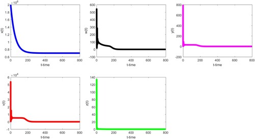
Table 2. Parameters used for simulation purpose.

Parameter	Value	Reference
λ	$1.4\times {10}^4$	Assumed
μ	0.02	[18]
β	$2.8\times {10}^{-8}$	[4]
δ	1.6	Assumed
η	0.18	Assumed
q	0.65	Assumed
α	1	[4]
p	2	Assumed
σ	4000	[4]
γ	23	[4]
k	0.1	Assumed
ρ	$1.5\times {10}^{-8}$	Assumed
c	3	[18]

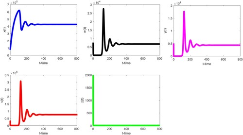
Secondly, we keep the values of the parameters as Table 2 except that δ is changed to 0.5 and k is changed to $5\times {10}^{-4}$. Then ${\mathcal{R}}_0=1.6659<1+\frac{q\mu \rho \lambda \sigma +\alpha \gamma \mu (\eta +q)}{\mu \delta \alpha \gamma }=2.7075$, ${\mathcal{R}}_1=0.8644<1$, and $c=3>k{y}_1=2.1542$. Therefore, all the assumptions of Theorem 3.5 are satisfied and hence the infected immune-free equilibrium $E_1=(4.2492\times {10}^5,6.6286\times {10}^3,4.3086\times {10}^3,7.4929\times {10}^5,0)$ is globally asymptotically stable. Figure 2 strongly supports this. In addition, we note that $x(t)$, $w(t)$, $y(t)$, and $v(t)$ start with severe fluctuations, and finally all tend to the stable values. While $z(t)$ decreases rapidly and is close to zero. This means that when the virus level in the body is low at the beginning, the body continues to carry out normal immune response, and healthy cells will continue to increase. With the increase, more healthy cells will be infected and the virus level will increase, which will lead to the decrease of healthy cells.

Figure 2. The infected immune-free equilibrium $E_1$ of (3(3) $\{\begin{array}{l}{\displaystyle \dot{x}(t)=\lambda -\mu x(t)-x(t)f(v(t))+\delta w(t),}\\ {\displaystyle \dot{w}(t)=x(t)f(v(t))-(\delta +\eta +q)w(t),}\\ {\displaystyle \dot{y}(t)=qw(t)-\alpha y(t)-py(t)z(t),}\\ {\displaystyle \dot{v}(t)=\sigma y(t)-\gamma v(t),}\\ {\displaystyle \dot{z}(t)=ky(t)z(t)-cz(t).}\end{array}$(3) ) is globally asymptotically stable when ${\mathcal{R}}_1<1<{\mathcal{R}}_0$. We refer to the text for details on parameter values and verification of other conditions.

Thirdly, we take the parameter values listed in Table 3. In this case, we have ${\mathcal{R}}_1=3.8929$ and $\mu (k\gamma +\rho c\sigma )(\delta +\eta +q)=6.045\times {10}^{-4}\ge \beta \delta \sigma c=6\times {10}^{-6}$. Therefore, Theorem 3.6 is applicable and we see that the infected equilibrium with immunity $E_2=(196.0992,1.9464,0.05,2.4997,0.1446)$ is globally asymptotically stable as demonstrated in Figure 3. Clearly, the values of $x(t)$, $w(t)$, $y(t)$, $v(t)$, and $z(t)$ are all greater than zero. We notice that $x(t)$ increases first and is close to be stable. $w(t)$ fluctuates obviously at the beginning, and then is stabilized. $y(t)$ and $v(t)$ decrease first, then fluctuate slightly, and tend to respective positive stable values. $z(t)$ increases first, then decreases and is close to the time axis, and finally tends towards the stable value after slight fluctuation. Unlike the previous two scenarios, $z(t)$ no longer coincides with the time axis. It shows that the patient's body produces a lot of CTLs.

Figure 3. With the parameter values in the text, we have ${\mathcal{R}}_1>1$ and $\mu x_2\ge \delta w_2$. Therefore, the infected equilibrium with immunity $E_2$ of (18(18) $\{\begin{array}{l}{\displaystyle \dot{x}=\lambda -\mu x-\frac{\beta xv}{1+\rho v}+\delta w,}\\ {\displaystyle \dot{w}=\frac{\beta xv}{1+\rho v}-(\delta +\eta +q)w,}\\ {\displaystyle \dot{y}=qw-\alpha y-pyz,}\\ {\displaystyle \dot{v}=\sigma y-\gamma v,}\\ {\displaystyle \dot{z}=kyz-cz.}\end{array}$(18) ) is globally asymptotically stable.

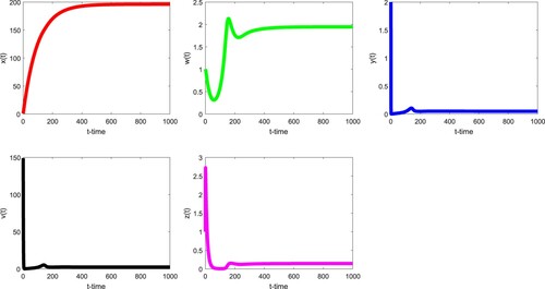
Table 3. Parameters used for simulation purpose.

Parameter	Value	Reference
λ	2	[18]
μ	0.01	[4]
β	$1.2\times {10}^{-4}$	[18]
δ	0.01	[18]
η	0.01	[18]
q	0.01	[18]
α	0.1	[18]
p	2	[18]
σ	50	[18]
γ	1	[18]
k	2	Assumed
ρ	0.003	Assumed
c	0.1	[18]

Finally, in Figure 4, we see that the infected immune-free equilibrium $E_1=(5.7285,97.1357,9.7136,485.6787,0)$ is globally asymptotically stable. However, the condition $\mu x_1\ge \delta w_1$ is not satisfied with ${\mathcal{R}}_0=40>1$, ${\mathcal{R}}_1=0.3294<1$ and $1+\frac{q\mu \rho \lambda \sigma +\alpha \gamma \mu (\eta +q)}{\mu \delta \alpha \gamma }=3.3$. Similarly, in Figure 5, we observe that the infected equilibrium with immunity $E_2$ is globally asymptotically stable. However, the condition $\mu x_2\ge \delta w_2$ is not satisfied with ${\mathcal{R}}_1=9.7525>1$ and $\mu (k\gamma +\rho c\sigma )(\delta +\eta +q)-\beta \delta \sigma c=-5.6955\times {10}^{-4}<0$. This may suggest that the technical conditions $\mu x_1\ge \delta w_1$ and $\mu x_2\ge \delta w_2$ may not be necessary for the global stability of $E_1$ and $E_2$, respectively (Tables 4 and 5).

Figure 4. With the parameter values in the Table 4, it is easy to verify that ${\mathcal{R}}_0=40>1+\frac{q\mu \rho \lambda \sigma +\alpha \gamma \mu (\eta +q)}{\mu \delta \alpha \gamma }=3.3$ and ${\mathcal{R}}_1=0.3294<1$. Therefore, the infected immune-free equilibrium $E_1$ of (3(3) $\{\begin{array}{l}{\displaystyle \dot{x}(t)=\lambda -\mu x(t)-x(t)f(v(t))+\delta w(t),}\\ {\displaystyle \dot{w}(t)=x(t)f(v(t))-(\delta +\eta +q)w(t),}\\ {\displaystyle \dot{y}(t)=qw(t)-\alpha y(t)-py(t)z(t),}\\ {\displaystyle \dot{v}(t)=\sigma y(t)-\gamma v(t),}\\ {\displaystyle \dot{z}(t)=ky(t)z(t)-cz(t).}\end{array}$(3) ) is globally asymptotically stable.

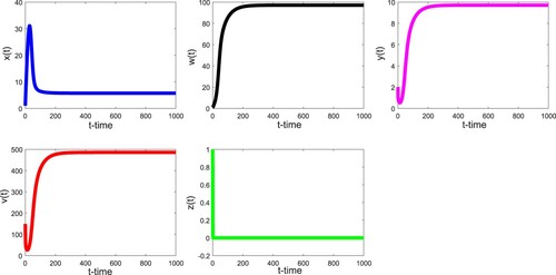
Figure 5. With the parameter values in the Table 5, it is easy to check that ${\mathcal{R}}_1=9.7525>1$ and the condition $\mu x_2\ge \delta w_2$ fails to hold.

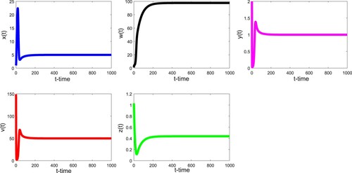
Table 4. Parameters used for simulation purpose.

Parameter	Value	Reference
λ	2	[18]
μ	0.01	[4]
β	$1.2\times {10}^{-3}$	[18]
δ	0.01	[18]
η	0.01	[18]
q	0.01	[18]
α	0.1	[18]
p	2	[18]
σ	50	[18]
γ	1	[18]
k	0.1	[18]
ρ	0.0003	[18]
c	3	[18]

Table 5. Parameters used for simulation purpose.

Parameter	Value	Reference
λ	2	[18]
μ	0.01	[4]
β	0.012	[18]
δ	0.01	[18]
η	0.01	[18]
q	0.01	[18]
α	0.1	[18]
p	2	[18]
σ	50	[18]
γ	1	[18]
k	0.1	[18]
ρ	0.0003	[18]
c	0.1	[18]

To conclude this section, we investigate the sensitivity of the basic reproduction number ${\mathcal{R}}_0$ and the basic immune reproduction ${\mathcal{R}}_1$ to all the parameters. The normalized forward sensitivity index of ${\mathcal{R}}_i$ with respect to a parameter p is defined as ${\zeta }_p=\frac{\mathrm{\partial }{\mathcal{R}}_i}{\mathrm{\partial }p}\frac{p}{{\mathcal{R}}_i},$where i = 0, 1. Table 6 summarizes the sensitivity indices of each parameter value. According to these indices, we obtain the relative changes of the basic reproduction numbers when the parameters of the model change, some of which are shown in Figure 6. For ${\mathcal{R}}_0$, the most sensitive parameters are λ, μ, β, α, σ and γ, followed by q, δ, and η, while k, ρ, and c have no effect on ${\mathcal{R}}_0$. But for ${\mathcal{R}}_1$, things are a little different. This time, all parameters affect ${\mathcal{R}}_1$, but only λ and α are the most sensitive parameters. The parameters μ, β, σ, γ, k, and c have almost the same effect. Furthermore, ${\mathcal{R}}_1$ is least sensitive to ρ.

Figure 6. Variations of the basic reproduction numbers with respect to the crucial parameters. All the parameter values are taken from Table 2. (a) λ. (b) α. (c) β. (d) σ. (e) η. (f) c

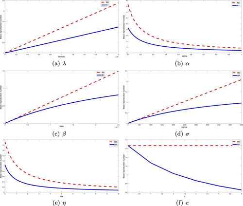
Table 6. The sensitivity indices of the basic reproduction number to the parameters.

Parameter	value	Sensitivity index of ${\mathcal{R}}_0$	Sensitivity index of ${\mathcal{R}}_1$
λ	$1.4\times {10}^4$	1	1
μ	0.02	$-1$	$-0.5270$
β	$2.8\times {10}^{-8}$	1	0.5270
δ	0.5	$-0.3759$	$-0.3268$
η	0.18	$-0.1353$	$-0.1739$
q	0.65	0.5113	0.3720
α	1	$-1$	$-1$
σ	4000	1	0.5189
γ	23	$-1$	$-0.5189$
k	$5\times {10}^{-4}$	0	0.4811
ρ	$1.5\times {10}^{-8}$	0	$-0.0081$
c	3	0	$-0.4811$

5. Conclusion

With the eclipse stage during HIV infection in consideration, we proposed a within-host HIV-1 infection model with a general incidence rate and CTL immune response, which can also be used to study the efficacy of treatment strategies by changing the corresponding parameters. The model is described by a system of five ordinary differential equations, which includes some in the literature as special cases, for example, those in [13, 18]. We found that the local dynamics is completely determined by the values of the two basic reproduction numbers, the basic infection reproduction number ${\mathcal{R}}_0$ and the basic immunity reproduction number ${\mathcal{R}}_1$. If ${\mathcal{R}}_0\le 1$, there is only the infection-free equilibrium $E_0$, which is locally asymptotically stable when ${\mathcal{R}}_0<1$; If ${\mathcal{R}}_1\le 1<{\mathcal{R}}_0$, besides $E_0$, there is also a unique infected immunity-free equilibrium $E_1=(x_1,w_1,y_1,v_1,0)$, which is locally asymptotically stable when ${\mathcal{R}}_1<1<{\mathcal{R}}_0$; if ${\mathcal{R}}_1>1$ (in this case, it is necessarily that ${\mathcal{R}}_0>1$), in addition to $E_0$ and $E_1$, there is a unique infection equilibrium with immunity $E_2=(x_2,w_2,y_2,v_2,z_2)$, which is locally asymptotically stable. Though we believe that the local dynamics also determines the global dynamics, we cannot confirm this so far. With the approach of Lyapunov functions, we have shown the global attractivity of the equilibria. If ${\mathcal{R}}_0\le 1$ then $E_0$ is globally attractive and hence the infection will be cleared; if ${\mathcal{R}}_0>1$ then the infection is persistent; if ${\mathcal{R}}_1>1$ then both infection and immunity will persist. Moreover, under some technical assumptions, we established the global stability of $E_1$ and $E_2$. More precisely, if ${\mathcal{R}}_1<1<{\mathcal{R}}_0$ and $\mu x_1\ge \delta w_1$, then $E_1$ is globally asymptotically stable. In this case, immunity cannot be established. But if ${\mathcal{R}}_1>1$ and $\mu x_2\ge \delta w_2$, then $E_2$ is globally asymptotically stable and hence infection and immunity will coexist. We should emphasize that, at that moment, the global stability of $E_1$ and $E_2$ are established under the technical conditions $\mu x_1\ge \delta w_1$ and $\mu x_2\ge \delta w_2$, respectively. When δ is very small, these technical conditions are satisfied. We also conducted some experiments without these technical conditions (see Figures 4 and 5). The numerical simulations suggest that both equilibria $E_1$ and $E_2$ may be globally asymptotically stable without the technical conditions. Unfortunately, we cannot confirm this yet and we leave it for future work.

We mention that some factors are ignored in our model. For example, some CTL populations can also attack infected cells during their eclipse stage [27]. With these factors incorporated, the analysis will be very complicated and so far we have not obtained any practicable theoretical results. This is one of our future works. On the other hand, minimizing the loss due to infections and the cost of treatments is also an important topic in infection dynamics. We shall construct reasonable objective functionals to investigate optimal problems.

Acknowledgments

This work was supported partially by the Funding for Outstanding Doctoral Dissertation in NUAA (No. BCXJ18-09), Postgraduate Research & Practice Innovation Program of Jiangsu Province (No. KYCX18_0234), and NSERC of Canada.

Disclosure statement

No potential conflict of interest was reported by the author(s).

Additional information

Funding

This work was supported by Postgraduate Research & Practice Innovation Program of Jiangsu Province [grant number KYCX18_0234] and NSERC of Canada and Funding for Outstanding Doctoral Dissertation in NUAA [grant number BCXJ18-09].

References

- P. Aavani and L.J.S. Allen, The role of CD4 T cells in immune system activation and viral reproduction in a simple model for HIV infection, Appl. Math. Model. 75 (2019), pp. 210–222.
- S. Ali, A.A. Raina, J. Iqbal, and R. Mathur, Mathematical modeling and stability analysis of HIV/AIDS-TB co-infection, Palest. J. Math. 8 (2019), pp. 380–391.
- D. Biswas and S. Palb, Stability analysis of a non-linear HIV/AIDS epidemic model with vaccination and antiretroviral therapy, Int. J. Adv. Appl. Math. Mech. 5 (2017), pp. 41–50.
- B. Buonomo and C. Vargas-De-León, Global stability for an HIV-1 infection model including an eclipse stage of infected cells, J. Math. Anal. Appl. 385 (2012), pp. 709–720.
- C. Castillo-Chavez and B. Song, Dynamical models of tuberculosis and their applications, Math. Biosci. Eng. 1 (2004), pp. 361–404.
- Q. Chen, Z. Teng, L. Wang, and H. Jiang, The existence of codimension-two bifurcation in a discrete SIS epidemic model with standard incidence, Nonlinear Dyn. 71 (2013), pp. 55–73.
- D. Ebert, C.D. Zschokke-Rohringer, and H.J. Carius, Dose effects and density-dependent regulation of two microparasites of Daphania magna, Oecologia 122 (2000), pp. 200–209.
- A.M. Elaiw and A.D. Al Agha, Stability of a general HIV-1 reaction-diffusion model with multiple delays and immune response, Phys. A 536 (2019), pp. 122593.
- N.R. Faria, A. Rambaut, M.A. Suchard, G. Baele, T. Bedford, M.J. Ward, A.J. Tatem, J.D. Sousa, N. Arinaminpathy, J. Pépin, D. Posada, M. Peeters, O.G. Pybus, and P. Lemey, The early spread and epidemic ignition of HIV-1 in human populations, Science 346 (2014), pp. 56–61.
- R.C. Gallo and L. Montagnier, The discovery of HIV as the cause of AIDS, N. Engl. J. Med. 349 (2003), pp. 2283–2285.
- M. Hesaaraki and M. Sabzevari, Global properties for an HIV-1 infection model including an eclipse stage of infected cells and saturation infection, Differ. Equ. Control Process. 4 (2013), pp. 67–83.
- A.L. Hill, D.I.S. Rosenbloom, M.A. Nowak, and R.F. Siliciano, Insight into treatment of HIV infection from viral dynamics models, Immunol. Rev. 285 (2018), pp. 9–25.
- Z. Hu, W. Pang, F. Liao, and W. Ma, Analysis of a CD4 + T cell viral infection model with a class of saturated infection rate, Discrete Contin. Dyn. Syst. Ser. B. 19 (2014), pp. 735–745.
- G. Kapitanov, C. Alvey, K. Vogt-Geisse, and Z. Feng, An age-structured model for the coupled dynamics of HIV and HSV-2, Math. Biosci. Eng. 12 (2015), pp. 803–840.
- X. Lai and X. Zou, Modeling cell-to-cell spread of HIV-1 with logistic target cell growth, J. Math. Anal. Appl. 426 (2015), pp. 563–584.
- J.P. LaSalle and S. Lefschetz, Stability by Lyapunov's Direct Method with Application, Academic Press, New York, 1961.
- B. Li, Y. Chen, X. Lu, and S. Liu, A delayed HIV-1 model with virus waning term, Math. Biosci. Eng. 13 (2016), pp. 135–157.
- C. Lv, L. Huang, and Z. Yuan, Global stability for an HIV-1 infection model with Beddington-DeAngelis incidence rate and CTL immune response, Commun. Nonlinear Sci. Numer. Simul. 19 (2014), pp. 121–127.
- N.J. Malunguza, S.D. Hove-Musekwa, S. Dube, and Z. Mukandavire, Dynamical properties and thresholds of an HIV model with super-infection, Math. Med. Biol. 34 (2017), pp. 493–522.
- M. Maziane, K. Hattaf, and N. Yousfi, Global stability of a class of HIV infection models with cure of infected cells in eclipse stage and CTL immune response, Int. J. Dynam. Control 5 (2017), pp. 1035–1045.
- P. Ngina, R.W. Mbogo, and L.S. Luboobi, HIV drug resistance: insights from mathematical modelling, Appl. Math. Model. 75 (2019), pp. 141–161.
- M. Nowak and C. Bangham, Population dynamics of immune responses to persistent viruses, Science272 (1996), pp. 74–79.
- E. Numfor, Optimal treatment in a multi-strain within-host model of HIV with age structure, J. Math. Anal. Appl. 480(2) (2019), pp. 123410.
- A. Nwankwo and D. Okuonghae, Mathematical analysis of the transmission dynamics of HIV syphilis co-infection in the presence of treatment for syphilis, Bull. Math. Biol. 80 (2018), pp. 437–492.
- A.S. Perelson and R.M. Ribeiro, Modeling the within-host dynamics of HIV infection, BMC Biol. 11 (2013), pp. 123. DOI:https://doi.org/10.1186/1741-7007-11-96.
- L. Rong, M.A. Gilchrist, Z. Feng, and A.S. Perelson, Modeling within-host HIV-1 dynamics and the evolution of drug resistance: trade-offs between viral enzyme function and drug susceptibility, J. Theoret. Biol. 247 (2007), pp. 804–818.
- J.B. Sacha, C. Chung, E.G. Rakasz, S.P. Spencer, A.K. Jonas, A.T. Bean, W. Lee, B.J. Burwitz, J.J.Stephany, J.T. Loffredo, D.B. Allison, S. Adnan, A. Hoji, N.A. Wilson, T.C. Friedrich, J.D. Lifson, O.O.Yang, and D.I. Watkins, Gag-specific CD8 + T lymphocytes recognize infected cells before AIDS-virus integration and viral protein expression, J. Immunol. 178(5) (2007), pp. 2746–2754.
- S.K. Sahani and Yashi, Effects of eclipse phase and delay on the dynamics of HIV infection, J. Biol. Syst. 26 (2018), pp. 421–454.
- M. Shen, Y. Xiao, and L. Rong, Global stability of an infection-age structured HIV-1 model linking within-host and between-host dynamics, Math. Biosci. 263 (2015), pp. 37–50.
- X. Song and A.U. Neumann, Global stability and periodic solution of the viral dynamics, J. Math. Anal. Appl. 329 (2007), pp. 281–297.
- J. Sotomayor, Generic Bifurcations of Dynamical Systems, Dynamical systems, Academic Press, 1973.
- N. Tarfulea, Drug therapy model with time delays for HIV infection with virus-to-cell and cell-to-cell transmissions, J. Appl. Math. Comput. 59 (2019), pp. 677–691.
- P. van den Driessche and J. Watmough, Reproduction numbers and sub-threshold endemic equilibria for compartmental models of disease transmission, Math. Biosci. 180 (2002), pp. 29–48.
- World Health Organization, HIV/AIDS, software. Available at https://www.who.int/news-room/fact-sheets/detail/hiv-aids.