Existence and stability of two periodic solutions for an interactive wild and sterile mosquitoes model

Abstract

In this paper, we study the periodic and stable dynamics of an interactive wild and sterile mosquito population model with density-dependent survival probability. We find a release amount upper bound $G^{\ast }$, depending on the release waiting period T, such that the model has exactly two periodic solutions, with one stable and another unstable, provided that the release amount does not exceed $G^{\ast }$. A numerical example is also given to illustrate our results.

Keywords:

• Sterile mosquitoes
• mosquito population suppression
• survival probability
• stability
• periodic solutions

AMS Subject Classifications:

• 34C25
• 34D20
• 34D23
• 92D25
• 93D20

1. Introduction

Mosquitoes have been listed as one of the deadliest animals around the world, due to their ability of transmitting mosquito-borne diseases through female mosquitoes' bitings. Take dengue as an example, the number of cases reported by World Health Organization increased dramatically over the last two decades, from 505,430 cases in 2000, to over 2.4 million in 2010, and 5.2 million in 2019 [30]. Since there have neither safe vaccines nor effective drugs to combat dengue, biological methods including Sterile Insect Technique (SIT) and Incompatible Insect Technique (IIT) have played vital roles in preventing the transmission of mosquito-borne diseases [1–5,8,11,19,27–29]. Both SIT and IIT involve releasing sterile male mosquitoes into the wild to mate with wild females, which result in no progeny for those females. It occurs that the number of wild mosquitoes will decrease gradually.

As sustainable and biologically safe approaches, the implementations of SIT, IIT and combined IIT-SIT for controlling wild mosquitoes are really acceptable and generalized. How to employ ideas of modelling to study the field has attracted great attention of many researchers, and various mathematical models have been formulated, we may refer to [6,20,21,32,34,38,39] for ordinary differential equations, [14,16,18,31,33,37] for delay differential equations, [9,15,17,22,23] for reaction-diffusion equations, [12,13] for stochastic equations, [25,26,35,36,40] for difference equations and references therein.

Based on a thought-provoking modelling idea proposed in [31] that the number of sterile mosquitoes at time t can be treated as a given function rather than an independent variable constrained by a differential equation, and by taking the fact that density-dependent death of wild mosquitoes mainly occurs in the aquatic stages (eggs, larvae, pupae)[7,24] into consideration, the authors in [21] studied the following ordinary differential equation model (1) $\begin{array}{r}\frac{\mathrm{d}w}{\mathrm{d}t}=\frac{a{w}^2(1-\xi w)}{w+g}-\mu w,\end{array}$(1) for exploring the interactive dynamics of wild and sterile mosquitoes. In model (1(1) $\begin{array}{r}\frac{\mathrm{d}w}{\mathrm{d}t}=\frac{a{w}^2(1-\xi w)}{w+g}-\mu w,\end{array}$(1) ), $w=w(t)$ and $g=g(t)$ denote the numbers of wild and sterile mosquitoes at time t, respectively, a is the maximum number of survived offspring produced per individual, $\frac{w}{w+g}$ is the mating probability between wild mosquitoes, ξ denotes the carrying capacity parameter such that $1-\xi w$ describes the density-dependent survival probability, and μ is the natural mortality of wild mosquitoes.

Although model (1(1) $\begin{array}{r}\frac{\mathrm{d}w}{\mathrm{d}t}=\frac{a{w}^2(1-\xi w)}{w+g}-\mu w,\end{array}$(1) ) looks simple, we find that it can generate rich dynamics. Obviously, $g(t)$ plays a key role in determining the asymptotic behaviours of model (1(1) $\begin{array}{r}\frac{\mathrm{d}w}{\mathrm{d}t}=\frac{a{w}^2(1-\xi w)}{w+g}-\mu w,\end{array}$(1) ), it is very important for us to make clear the structure of $g(t)$. To this end, let $\overline{T}$ and T be the sexual lifespan of released sterile mosquitoes and the waiting period between two consecutive releases, respectively. Then there exists three different release strategies: $T=\overline{T}$, $T>\overline{T}$, and $T<\overline{T}$. Moreover, we assume that the release begins at time t = 0 such that $g(t)=0$ for t<0, and a constant amount c of sterile mosquitoes is impulsively and periodically released at discrete time points $T_i=iT,i=0,1,2,\dots$. When $T=\overline{T}$, $g(t)\equiv c$ for all $t\ge 0$. And model (1(1) $\begin{array}{r}\frac{\mathrm{d}w}{\mathrm{d}t}=\frac{a{w}^2(1-\xi w)}{w+g}-\mu w,\end{array}$(1) ) with $g(t)\equiv c$ has been investigated in [21]. For the case when $T>\overline{T}$, we have $\begin{array}{r}g(t)=\{\begin{array}{l}c,t\in [iT,iT+\overline{T}),\\ 0,t\in [iT+\overline{T},(i+1)T),\end{array}i=0,1,2,\dots ,\end{array}$ and model (1(1) $\begin{array}{r}\frac{\mathrm{d}w}{\mathrm{d}t}=\frac{a{w}^2(1-\xi w)}{w+g}-\mu w,\end{array}$(1) ) becomes $\begin{array}{r}\{\begin{array}{lll}{\displaystyle \frac{\mathrm{d}w}{\mathrm{d}t}}& ={\displaystyle \frac{a{w}^2(1-\xi w)}{w+c}}-\mu w,& t\in [iT,iT+\overline{T}),\\ {\displaystyle \frac{\mathrm{d}w}{\mathrm{d}t}}& =-a\xi w(w-A),& t\in [iT+\overline{T},(i+1)T),\end{array}i=0,1,2,\dots ,\end{array}$ which has recently been discussed in [43], where $A=\frac{a-\mu }{a\xi }$.

We study the release strategy of $T<\overline{T}$ in this paper. Let $[x]$ represent the largest integer portion of x. Then there exists an integer $j=j(T)$ and a nonnegative number $r=r(T)\in [0,T)$ such that $\overline{T}=jT+r$. When $t\in [0,jT)$, we get $\begin{array}{r}g(t)=ic,t\in [(i-1)T,iT),i=1,2,\dots ,j.\end{array}$ When $t\ge jT$, if r = 0, then $g(t)=jc$, under which model (1(1) $\begin{array}{r}\frac{\mathrm{d}w}{\mathrm{d}t}=\frac{a{w}^2(1-\xi w)}{w+g}-\mu w,\end{array}$(1) ) can be reduced to the one in [21]. If $r\ne 0$, then (2) $\begin{array}{r}g(t)=\{\begin{array}{ll}(j+1)c,& t\in [(i-1)T,(i-1)T+r),\\ jc,& t\in [(i-1)T+r,iT),\end{array}i=j+1,j+2,\dots .\end{array}$(2) See Figure 1 for illustration. Then model (1(1) $\begin{array}{r}\frac{\mathrm{d}w}{\mathrm{d}t}=\frac{a{w}^2(1-\xi w)}{w+g}-\mu w,\end{array}$(1) ) reads as $\begin{array}{rl}& \frac{\mathrm{d}w}{\mathrm{d}t}=\frac{a{w}^2(1-\xi w)}{w+ic}-\mu w,t\in [(i-1)T,iT),i=1,2,\cdots ,j,\\ & \begin{array}{rl}& \frac{\mathrm{d}w}{\mathrm{d}t}=\frac{a{w}^2(1-\xi w)}{w+(j+1)c}-\mu w,t\in [(i-1)T,(i-1)T+r)\\ & \frac{\mathrm{d}w}{\mathrm{d}t}=\frac{a{w}^2(1-\xi w)}{w+jc}-\mu w,t\in [(i-1)T+r,iT)\end{array}\},i=j+1,j+2,\cdots .\end{array}$

Figure 1. A schematic illustration for figuring out the structure of $g(t)$.

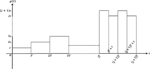
We assume 0<r<T in the remaining of this paper. Since our main concern is the asymptotic dynamics of the model, we may assume that the initial time point is $t_0=jT$. Then $g(t)$ takes the form of (2(2) $\begin{array}{r}g(t)=\{\begin{array}{ll}(j+1)c,& t\in [(i-1)T,(i-1)T+r),\\ jc,& t\in [(i-1)T+r,iT),\end{array}i=j+1,j+2,\dots .\end{array}$(2) ).

Let the release amount upper bound $G^{\ast }$ be defined as $\begin{array}{r}{G}^{\ast }=\frac{(a-\mu {)}^2}{4a\mu \xi (j+1)}.\end{array}$ Then model (1(1) $\begin{array}{r}\frac{\mathrm{d}w}{\mathrm{d}t}=\frac{a{w}^2(1-\xi w)}{w+g}-\mu w,\end{array}$(1) ) can be rewritten as (3) $\begin{array}{r}\{\begin{array}{l}\begin{array}{rl}\frac{\mathrm{d}w}{\mathrm{d}t}& =-\frac{a\xi w}{w+(j+1)c}[{(w-\frac{A}{2})}^2+\frac{\mu (j+1)}{a\xi }(c-G^{\ast })],t\in [(i-1)T,(i-1)T+r),\\ \frac{\mathrm{d}w}{\mathrm{d}t}& =-\frac{a\xi w}{w+jc}[{(w-\frac{A}{2})}^2+\frac{\mu j}{a\xi }(c-\frac{j+1}{j}{G}^{\ast })],t\in [(i-1)T+r,iT),\end{array}\end{array}\end{array}$(3)

$i=j+1,j+2,\dots$.

We, in this paper, mainly study the long-time dynamics of model (3(3) $\begin{array}{r}\{\begin{array}{l}\begin{array}{rl}\frac{\mathrm{d}w}{\mathrm{d}t}& =-\frac{a\xi w}{w+(j+1)c}[{(w-\frac{A}{2})}^2+\frac{\mu (j+1)}{a\xi }(c-G^{\ast })],t\in [(i-1)T,(i-1)T+r),\\ \frac{\mathrm{d}w}{\mathrm{d}t}& =-\frac{a\xi w}{w+jc}[{(w-\frac{A}{2})}^2+\frac{\mu j}{a\xi }(c-\frac{j+1}{j}{G}^{\ast })],t\in [(i-1)T+r,iT),\end{array}\end{array}\end{array}$(3) ) under the assumptions of $T<\overline{T}$ and $0<c\le G^{\ast }$. The paper is arranged as follows. In Section 2, we define the Poincaré map and give three lemmas. In Section 3, the theoretical results show that if $0<c\le G^{\ast }$, then the model has exactly two T-periodic solutions, with one stable and another unstable. Finally, a brief discussion is given in Section 4.

2. Preliminaries

It is apparent that the origin, denoted by $w_0$, is the unique equilibrium of model (3(3) $\begin{array}{r}\{\begin{array}{l}\begin{array}{rl}\frac{\mathrm{d}w}{\mathrm{d}t}& =-\frac{a\xi w}{w+(j+1)c}[{(w-\frac{A}{2})}^2+\frac{\mu (j+1)}{a\xi }(c-G^{\ast })],t\in [(i-1)T,(i-1)T+r),\\ \frac{\mathrm{d}w}{\mathrm{d}t}& =-\frac{a\xi w}{w+jc}[{(w-\frac{A}{2})}^2+\frac{\mu j}{a\xi }(c-\frac{j+1}{j}{G}^{\ast })],t\in [(i-1)T+r,iT),\end{array}\end{array}\end{array}$(3) ). We first give the definition of a solution of model (3(3) $\begin{array}{r}\{\begin{array}{l}\begin{array}{rl}\frac{\mathrm{d}w}{\mathrm{d}t}& =-\frac{a\xi w}{w+(j+1)c}[{(w-\frac{A}{2})}^2+\frac{\mu (j+1)}{a\xi }(c-G^{\ast })],t\in [(i-1)T,(i-1)T+r),\\ \frac{\mathrm{d}w}{\mathrm{d}t}& =-\frac{a\xi w}{w+jc}[{(w-\frac{A}{2})}^2+\frac{\mu j}{a\xi }(c-\frac{j+1}{j}{G}^{\ast })],t\in [(i-1)T+r,iT),\end{array}\end{array}\end{array}$(3) ). A function $w(t)$ is said to be a solution of model (3(3) $\begin{array}{r}\{\begin{array}{l}\begin{array}{rl}\frac{\mathrm{d}w}{\mathrm{d}t}& =-\frac{a\xi w}{w+(j+1)c}[{(w-\frac{A}{2})}^2+\frac{\mu (j+1)}{a\xi }(c-G^{\ast })],t\in [(i-1)T,(i-1)T+r),\\ \frac{\mathrm{d}w}{\mathrm{d}t}& =-\frac{a\xi w}{w+jc}[{(w-\frac{A}{2})}^2+\frac{\mu j}{a\xi }(c-\frac{j+1}{j}{G}^{\ast })],t\in [(i-1)T+r,iT),\end{array}\end{array}\end{array}$(3) ) if it satisfies the first equation of model (3(3) $\begin{array}{r}\{\begin{array}{l}\begin{array}{rl}\frac{\mathrm{d}w}{\mathrm{d}t}& =-\frac{a\xi w}{w+(j+1)c}[{(w-\frac{A}{2})}^2+\frac{\mu (j+1)}{a\xi }(c-G^{\ast })],t\in [(i-1)T,(i-1)T+r),\\ \frac{\mathrm{d}w}{\mathrm{d}t}& =-\frac{a\xi w}{w+jc}[{(w-\frac{A}{2})}^2+\frac{\mu j}{a\xi }(c-\frac{j+1}{j}{G}^{\ast })],t\in [(i-1)T+r,iT),\end{array}\end{array}\end{array}$(3) ) on $[(i-1)T,(i-1)T+r)$, and the second equation of model (3(3) $\begin{array}{r}\{\begin{array}{l}\begin{array}{rl}\frac{\mathrm{d}w}{\mathrm{d}t}& =-\frac{a\xi w}{w+(j+1)c}[{(w-\frac{A}{2})}^2+\frac{\mu (j+1)}{a\xi }(c-G^{\ast })],t\in [(i-1)T,(i-1)T+r),\\ \frac{\mathrm{d}w}{\mathrm{d}t}& =-\frac{a\xi w}{w+jc}[{(w-\frac{A}{2})}^2+\frac{\mu j}{a\xi }(c-\frac{j+1}{j}{G}^{\ast })],t\in [(i-1)T+r,iT),\end{array}\end{array}\end{array}$(3) ) on $[(i-1)T+r,iT),i=j+1,j+2,\dots$ [10]. Let $w(t)=w(t;jT,u)$ denote the solution of model (3(3) $\begin{array}{r}\{\begin{array}{l}\begin{array}{rl}\frac{\mathrm{d}w}{\mathrm{d}t}& =-\frac{a\xi w}{w+(j+1)c}[{(w-\frac{A}{2})}^2+\frac{\mu (j+1)}{a\xi }(c-G^{\ast })],t\in [(i-1)T,(i-1)T+r),\\ \frac{\mathrm{d}w}{\mathrm{d}t}& =-\frac{a\xi w}{w+jc}[{(w-\frac{A}{2})}^2+\frac{\mu j}{a\xi }(c-\frac{j+1}{j}{G}^{\ast })],t\in [(i-1)T+r,iT),\end{array}\end{array}\end{array}$(3) ) with initial value $w(jT)=u>0$. Furthermore, we define $w(iT)=w((iT{)}^{-})$ and $w(iT+r)=w((iT+r{)}^{-})$ for $i=j+1,j+2,\dots$. Then $w(t)$ is a continuous and piecewise differentiable function defined on $[jT,\mathrm{\infty })$.

Set the two auxiliary functions $\overline{h}(u)$ and $h(u)$ be defined as $\begin{array}{r}\overline{h}(u)=w(jT+r;jT,u),\mathrm{and}h(u)=w((j+1)T;jT,u).\end{array}$ Clearly, both $\overline{h}(u)$ and $h(u)$ are continuous and differentiable on $[0,+\mathrm{\infty })$. A T-periodic solution occurs if $w((j+1)T;jT,u)=u$, i.e. $h(u)=u$. Consequently, existence of fixed points of h ensures existence of T-periodic solutions of model (3(3) $\begin{array}{r}\{\begin{array}{l}\begin{array}{rl}\frac{\mathrm{d}w}{\mathrm{d}t}& =-\frac{a\xi w}{w+(j+1)c}[{(w-\frac{A}{2})}^2+\frac{\mu (j+1)}{a\xi }(c-G^{\ast })],t\in [(i-1)T,(i-1)T+r),\\ \frac{\mathrm{d}w}{\mathrm{d}t}& =-\frac{a\xi w}{w+jc}[{(w-\frac{A}{2})}^2+\frac{\mu j}{a\xi }(c-\frac{j+1}{j}{G}^{\ast })],t\in [(i-1)T+r,iT),\end{array}\end{array}\end{array}$(3) ). For characterizing the asymptotic behaviours of solutions, we define sequences $\{{\overline{h}}_n\}$ and $\{h_n\}$ by (4) $\begin{array}{r}{\overline{h}}_n(u)=w(nT+jT+r;jT,u),h_n(u)=w(nT+jT;jT,u),n=0,1,2,\dots ,\end{array}$(4) which satisfy $\begin{array}{r}{\overline{h}}_0(u)=w(jT+r;jT,u),h_0(u)=u,{\overline{h}}_n(u)=\overline{h}(h_n(u)),h_{n+1}(u)=h(h_n(u)),\end{array}$ for $n=0,1,2,\dots$, see [34] for details. Following the lines in [34], for sequences defined in (4(4) $\begin{array}{r}{\overline{h}}_n(u)=w(nT+jT+r;jT,u),h_n(u)=w(nT+jT;jT,u),n=0,1,2,\dots ,\end{array}$(4) ), we may similarly obtain the next lemma.

Lemma 2.1

For any given initial value u>0, the following conclusions hold.

(1)	If $h(u)>u$, then sequences $\{h_n(u)\}$ and $\{{\overline{h}}_n(u)\}$ are both strictly increasing;
(2)	If $h(u)=u$, then $h_n(u)\equiv u$ for $n=0,1,2,\dots$;
(3)	If $h(u)<u$, then sequences $\{h_n(u)\}$ and $\{{\overline{h}}_n(u)\}$ are both strictly decreasing.

By a similar argument to that in the proof of Lemma 2.9 in [32], we arrive at the following lemma, which provides a necessary and sufficient condition for the origin $w_0$ to be asymptotically stable.

Lemma 2.2

The origin $w_0$ is asymptotically stable if and only if there is ${\delta }_0>0$ such that $\begin{array}{r}h(u)<u,\mathrm{for}u\in (0,{\delta }_0).\end{array}$

Since our focus is to find the fixed points of h, we need to know the different relationships between $h(u)$ and u for all u>0. Moreover, from Lemmas 2.1 and 2.2, we find that the sign of $h^{\prime }(u)-1$ is crucial to the comparison between $h(u)$ and u. To obtain the expression for $h^{\prime }(u)$, we will first solve the first equation of model (3(3) $\begin{array}{r}\{\begin{array}{l}\begin{array}{rl}\frac{\mathrm{d}w}{\mathrm{d}t}& =-\frac{a\xi w}{w+(j+1)c}[{(w-\frac{A}{2})}^2+\frac{\mu (j+1)}{a\xi }(c-G^{\ast })],t\in [(i-1)T,(i-1)T+r),\\ \frac{\mathrm{d}w}{\mathrm{d}t}& =-\frac{a\xi w}{w+jc}[{(w-\frac{A}{2})}^2+\frac{\mu j}{a\xi }(c-\frac{j+1}{j}{G}^{\ast })],t\in [(i-1)T+r,iT),\end{array}\end{array}\end{array}$(3) ) with initial value $w(jT)=u$ for getting the expression of ${\overline{h}}^{\prime }(u)$, then solve the second equation of model (3(3) $\begin{array}{r}\{\begin{array}{l}\begin{array}{rl}\frac{\mathrm{d}w}{\mathrm{d}t}& =-\frac{a\xi w}{w+(j+1)c}[{(w-\frac{A}{2})}^2+\frac{\mu (j+1)}{a\xi }(c-G^{\ast })],t\in [(i-1)T,(i-1)T+r),\\ \frac{\mathrm{d}w}{\mathrm{d}t}& =-\frac{a\xi w}{w+jc}[{(w-\frac{A}{2})}^2+\frac{\mu j}{a\xi }(c-\frac{j+1}{j}{G}^{\ast })],t\in [(i-1)T+r,iT),\end{array}\end{array}\end{array}$(3) ) with initial value $w(jT+r)=\overline{h}(u)$ to get the relationship between ${\overline{h}}^{\prime }(u)$ and $h^{\prime }(u)$. To go ahead without the burden of frequently switching between the first equation and the second equation of model (3(3) $\begin{array}{r}\{\begin{array}{l}\begin{array}{rl}\frac{\mathrm{d}w}{\mathrm{d}t}& =-\frac{a\xi w}{w+(j+1)c}[{(w-\frac{A}{2})}^2+\frac{\mu (j+1)}{a\xi }(c-G^{\ast })],t\in [(i-1)T,(i-1)T+r),\\ \frac{\mathrm{d}w}{\mathrm{d}t}& =-\frac{a\xi w}{w+jc}[{(w-\frac{A}{2})}^2+\frac{\mu j}{a\xi }(c-\frac{j+1}{j}{G}^{\ast })],t\in [(i-1)T+r,iT),\end{array}\end{array}\end{array}$(3) ), we rewrite model (3(3) $\begin{array}{r}\{\begin{array}{l}\begin{array}{rl}\frac{\mathrm{d}w}{\mathrm{d}t}& =-\frac{a\xi w}{w+(j+1)c}[{(w-\frac{A}{2})}^2+\frac{\mu (j+1)}{a\xi }(c-G^{\ast })],t\in [(i-1)T,(i-1)T+r),\\ \frac{\mathrm{d}w}{\mathrm{d}t}& =-\frac{a\xi w}{w+jc}[{(w-\frac{A}{2})}^2+\frac{\mu j}{a\xi }(c-\frac{j+1}{j}{G}^{\ast })],t\in [(i-1)T+r,iT),\end{array}\end{array}\end{array}$(3) ) as follows (5) $\begin{array}{r}\frac{\mathrm{d}w}{\mathrm{d}t}=-\frac{a\xi w}{w+kc}[{(w-\frac{A}{2})}^2+\frac{\mu k}{a\xi }(c-g^{\ast }(k))]\triangleq f(w),\end{array}$(5) with k = j + 1 when $t\in [(i-1)T,(i-1)T+r)$, or k = j when $t\in [(i-1)T+r,iT)$, where $i=j+1,j+2,\dots$, and $g^{\ast }(k)=\frac{(a-\mu {)}^2}{4ak\mu \xi }$.

Since $0<c\le G^{\ast }\le g^{\ast }(k)$, we know that $f(w)=0$ has two positive real roots. Denote the two roots by $E_1(k,c)$ and $E_2(k,c)$, then $\begin{array}{r}{E}_1(k,c)=\frac{A}{2}-\sqrt{\frac{\mu k}{a\xi }(g^{\ast }(k)-c)},E_2(k,c)=\frac{A}{2}+\sqrt{\frac{\mu k}{a\xi }(g^{\ast }(k)-c)}.\end{array}$ Moreover, we have (6) $\begin{array}{r}{E}_1(j,c)<E_1(j+1,c)<E_2(j+1,c)<E_2(j,c).\end{array}$(6) By letting ${\delta }_0=E_1(j,c)$ in Lemma 2.2, and using (3(3) $\begin{array}{r}\{\begin{array}{l}\begin{array}{rl}\frac{\mathrm{d}w}{\mathrm{d}t}& =-\frac{a\xi w}{w+(j+1)c}[{(w-\frac{A}{2})}^2+\frac{\mu (j+1)}{a\xi }(c-G^{\ast })],t\in [(i-1)T,(i-1)T+r),\\ \frac{\mathrm{d}w}{\mathrm{d}t}& =-\frac{a\xi w}{w+jc}[{(w-\frac{A}{2})}^2+\frac{\mu j}{a\xi }(c-\frac{j+1}{j}{G}^{\ast })],t\in [(i-1)T+r,iT),\end{array}\end{array}\end{array}$(3) ) and (6(6) $\begin{array}{r}{E}_1(j,c)<E_1(j+1,c)<E_2(j+1,c)<E_2(j,c).\end{array}$(6) ), we have the following lemma.

Lemma 2.3

The origin $w_0$ is always locally asymptotically stable.

Biologically, Lemma 2.3 means that the suppression on wild mosquitoes is always successful provided that the initial density of wild mosquitoes is contained within the region of attraction of $w_0$.

Recall that the sign of $h^{\prime }(u)-1$ is our deepest concern, and to get this sign, it suffices to obtain the expression for $h^{\prime }(u)$. In the following, we are devoted to seeking the expression. To this end, we need to consider the following two cases.

Case 1: $0<c<G^{\ast }$. In this case, Equation (5(5) $\begin{array}{r}\frac{\mathrm{d}w}{\mathrm{d}t}=-\frac{a\xi w}{w+kc}[{(w-\frac{A}{2})}^2+\frac{\mu k}{a\xi }(c-g^{\ast }(k))]\triangleq f(w),\end{array}$(5) ) can be transformed to (7) $\begin{array}{r}\frac{w+kc}{w({(w-\frac{A}{2})}^2-\frac{\mu k}{a\xi }(g^{\ast }(k)-c))}\mathrm{d}w=-a\xi \mathrm{d}t.\end{array}$(7) By partial fraction decomposition of $w((w-\frac{A}{2}{)}^2-\frac{\mu k}{a\xi }(g^{\ast }(k)-c))$, (7(7) $\begin{array}{r}\frac{w+kc}{w({(w-\frac{A}{2})}^2-\frac{\mu k}{a\xi }(g^{\ast }(k)-c))}\mathrm{d}w=-a\xi \mathrm{d}t.\end{array}$(7) ) gives (8) $\begin{array}{r}(\frac{{\alpha }_1(k)}{w}+\frac{{\beta }_1(k)}{w-E_1(k,c)}+\frac{{\gamma }_1(k)}{w-E_2(k,c)})\mathrm{d}w=-a\xi \mathrm{d}t,\end{array}$(8) where $\begin{array}{rl}{\alpha }_1(k)& =\frac{kc}{E_1(k,c)E_2(k,c)},{\beta }_1(k)=-\frac{kc+E_1(k,c)}{E_1(k,c)(E_2(k,c)-E_1(k,c))},\\ {\gamma }_1(k)& =\frac{kc+E_2(k,c)}{E_2(k,c)(E_2(k,c)-E_1(k,c))}.\end{array}$ Making the identity transformation for (8(8) $\begin{array}{r}(\frac{{\alpha }_1(k)}{w}+\frac{{\beta }_1(k)}{w-E_1(k,c)}+\frac{{\gamma }_1(k)}{w-E_2(k,c)})\mathrm{d}w=-a\xi \mathrm{d}t,\end{array}$(8) ), we get (9) $\begin{array}{r}\mathrm{d}[\ln (w^{{\alpha }_1(k)}\cdot {|w-E_1(k,c)|}^{{\beta }_1(k)}\cdot {|w-E_2(k,c)|}^{{\gamma }_1(k)})]=-a\xi \mathrm{d}t.\end{array}$(9) Integrating (9(9) $\begin{array}{r}\mathrm{d}[\ln (w^{{\alpha }_1(k)}\cdot {|w-E_1(k,c)|}^{{\beta }_1(k)}\cdot {|w-E_2(k,c)|}^{{\gamma }_1(k)})]=-a\xi \mathrm{d}t.\end{array}$(9) ) from jT to jT + r with k = j + 1, and recall that (10) $\begin{array}{r}w(jT)=u,w(jT+r)=\overline{h}(u),\end{array}$(10) we have (11) $\begin{array}{r}\frac{{\overline{h}}^{{\alpha }_1(k)}\left(u\right)\cdot {|\overline{h}\left(u\right)-E_1(j+1,c)|}^{{\beta }_1(k)}\cdot {|\overline{h}\left(u\right)-E_2(j+1,c)|}^{{\gamma }_1(k)}}{u^{{\alpha }_1(k)}\cdot {|u-E_1(j+1,c)|}^{{\beta }_1(k)}\cdot {|u-E_2(j+1,c)|}^{{\gamma }_1(k)}}=e^{-a\xi r}.\end{array}$(11) For notation simplicity, let (12) $\begin{array}{r}{L}_1(u,k)=u^{{\alpha }_1(k)}\cdot {|u-E_1(k,c)|}^{{\beta }_1(k)}\cdot {|u-E_2(k,c)|}^{{\gamma }_1(k)}.\end{array}$(12) Taking the partial derivative with respect to u of both sides of (12(12) $\begin{array}{r}{L}_1(u,k)=u^{{\alpha }_1(k)}\cdot {|u-E_1(k,c)|}^{{\beta }_1(k)}\cdot {|u-E_2(k,c)|}^{{\gamma }_1(k)}.\end{array}$(12) ), we get (13) $\begin{array}{r}\frac{\mathrm{\partial }{L}_1(u,k)}{\mathrm{\partial }u}=L_1(u,k)\frac{u+kc}{u(u-E_1(k,c))(u-E_2(k,c))}.\end{array}$(13) Furthermore, substituting (12(12) $\begin{array}{r}{L}_1(u,k)=u^{{\alpha }_1(k)}\cdot {|u-E_1(k,c)|}^{{\beta }_1(k)}\cdot {|u-E_2(k,c)|}^{{\gamma }_1(k)}.\end{array}$(12) ) and k = j + 1 into (11(11) $\begin{array}{r}\frac{{\overline{h}}^{{\alpha }_1(k)}\left(u\right)\cdot {|\overline{h}\left(u\right)-E_1(j+1,c)|}^{{\beta }_1(k)}\cdot {|\overline{h}\left(u\right)-E_2(j+1,c)|}^{{\gamma }_1(k)}}{u^{{\alpha }_1(k)}\cdot {|u-E_1(j+1,c)|}^{{\beta }_1(k)}\cdot {|u-E_2(j+1,c)|}^{{\gamma }_1(k)}}=e^{-a\xi r}.\end{array}$(11) ), we have (14) $\begin{array}{r}{L}_1(\overline{h}\left(u\right),j+1)=L_1(u,j+1)e^{-a\xi r}.\end{array}$(14) To get the expression for ${\overline{h}}^{\prime }(u)$, we take the derivative with respect to u of both sides of (14(14) $\begin{array}{r}{L}_1(\overline{h}\left(u\right),j+1)=L_1(u,j+1)e^{-a\xi r}.\end{array}$(14) ), which yields (15) $\begin{array}{r}\frac{\mathrm{\partial }{L}_1(\overline{h}\left(u\right),j+1)}{\mathrm{\partial }\overline{h}(u)}{\overline{h}}^{\prime }(u)=\frac{\mathrm{\partial }{L}_1(u,j+1)}{\mathrm{\partial }u}{e}^{-a\xi r}.\end{array}$(15) Substituting (13(13) $\begin{array}{r}\frac{\mathrm{\partial }{L}_1(u,k)}{\mathrm{\partial }u}=L_1(u,k)\frac{u+kc}{u(u-E_1(k,c))(u-E_2(k,c))}.\end{array}$(13) ) with k = j + 1 and (14(14) $\begin{array}{r}{L}_1(\overline{h}\left(u\right),j+1)=L_1(u,j+1)e^{-a\xi r}.\end{array}$(14) ) into (15(15) $\begin{array}{r}\frac{\mathrm{\partial }{L}_1(\overline{h}\left(u\right),j+1)}{\mathrm{\partial }\overline{h}(u)}{\overline{h}}^{\prime }(u)=\frac{\mathrm{\partial }{L}_1(u,j+1)}{\mathrm{\partial }u}{e}^{-a\xi r}.\end{array}$(15) ), we obtain (16) $\begin{array}{rl}& \frac{\overline{h}(u)+(j+1)c}{\overline{h}\left(u\right)(\overline{h}\left(u\right)-E_1(j+1,c))(\overline{h}\left(u\right)-E_2(j+1,c))}{\overline{h}}^{\prime }\left(u\right)=\frac{u+(j+1)c}{u(u-E_1(j+1,c))(u-E_2(j+1,c))}.\end{array}$(16)

For the solution going from $\overline{h}(u)$ to $h(u)$, we integrate (9(9) $\begin{array}{r}\mathrm{d}[\ln (w^{{\alpha }_1(k)}\cdot {|w-E_1(k,c)|}^{{\beta }_1(k)}\cdot {|w-E_2(k,c)|}^{{\gamma }_1(k)})]=-a\xi \mathrm{d}t.\end{array}$(9) ) from jT + r to $(j+1)T$ with k = j, which reaches (17) $\begin{array}{r}\frac{h^{{\alpha }_1(k)}\left(u\right)\cdot {|h\left(u\right)-E_1(j,c)|}^{{\beta }_1(k)}\cdot {|h\left(u\right)-E_2(j,c)|}^{{\gamma }_1(k)}}{{\overline{h}}^{{\alpha }_1(k)}\left(u\right)\cdot {|\overline{h}\left(u\right)-E_1(j,c)|}^{{\beta }_1(k)}\cdot {|\overline{h}\left(u\right)-E_2(j,c)|}^{{\gamma }_1(k)}}=e^{-a\xi (T-r)}.\end{array}$(17) By (12(12) $\begin{array}{r}{L}_1(u,k)=u^{{\alpha }_1(k)}\cdot {|u-E_1(k,c)|}^{{\beta }_1(k)}\cdot {|u-E_2(k,c)|}^{{\gamma }_1(k)}.\end{array}$(12) ) and k = j, (17(17) $\begin{array}{r}\frac{h^{{\alpha }_1(k)}\left(u\right)\cdot {|h\left(u\right)-E_1(j,c)|}^{{\beta }_1(k)}\cdot {|h\left(u\right)-E_2(j,c)|}^{{\gamma }_1(k)}}{{\overline{h}}^{{\alpha }_1(k)}\left(u\right)\cdot {|\overline{h}\left(u\right)-E_1(j,c)|}^{{\beta }_1(k)}\cdot {|\overline{h}\left(u\right)-E_2(j,c)|}^{{\gamma }_1(k)}}=e^{-a\xi (T-r)}.\end{array}$(17) ) becomes (18) $\begin{array}{r}{L}_1(h\left(u\right),j)=L_1(\overline{h}\left(u\right),j)e^{-a\xi (T-r)}.\end{array}$(18) Similarly, to get $h^{\prime }(u)$, we take the derivative with respect to u of both sides of (18(18) $\begin{array}{r}{L}_1(h\left(u\right),j)=L_1(\overline{h}\left(u\right),j)e^{-a\xi (T-r)}.\end{array}$(18) ), which gives (19) $\begin{array}{r}\frac{\mathrm{\partial }{L}_1(h\left(u\right),j)}{\mathrm{\partial }h\left(u\right)}{h}^{\prime }\left(u\right)=\frac{\mathrm{\partial }{L}_1(\overline{h}\left(u\right),j)}{\mathrm{\partial }\overline{h}(u)}{\overline{h}}^{\prime }\left(u\right)e^{-a\xi (T-r)}.\end{array}$(19) Substituting (12(12) $\begin{array}{r}{L}_1(u,k)=u^{{\alpha }_1(k)}\cdot {|u-E_1(k,c)|}^{{\beta }_1(k)}\cdot {|u-E_2(k,c)|}^{{\gamma }_1(k)}.\end{array}$(12) ) with k = j and (18(18) $\begin{array}{r}{L}_1(h\left(u\right),j)=L_1(\overline{h}\left(u\right),j)e^{-a\xi (T-r)}.\end{array}$(18) ) into (19(19) $\begin{array}{r}\frac{\mathrm{\partial }{L}_1(h\left(u\right),j)}{\mathrm{\partial }h\left(u\right)}{h}^{\prime }\left(u\right)=\frac{\mathrm{\partial }{L}_1(\overline{h}\left(u\right),j)}{\mathrm{\partial }\overline{h}(u)}{\overline{h}}^{\prime }\left(u\right)e^{-a\xi (T-r)}.\end{array}$(19) ), we get (20) $\begin{array}{r}\frac{(h\left(u\right)+jc)h^{\prime }\left(u\right)}{h\left(u\right)(h\left(u\right)-E_1(j,c))(h\left(u\right)-E_2(j,c))}=\frac{(\overline{h}\left(u\right)+jc){\overline{h}}^{\prime }\left(u\right)}{\overline{h}\left(u\right)(\overline{h}\left(u\right)-E_1(j,c))(\overline{h}\left(u\right)-E_2(j,c))}.\end{array}$(20)

Case 2: $c=G^{\ast }$. In this case, Equation (5(5) $\begin{array}{r}\frac{\mathrm{d}w}{\mathrm{d}t}=-\frac{a\xi w}{w+kc}[{(w-\frac{A}{2})}^2+\frac{\mu k}{a\xi }(c-g^{\ast }(k))]\triangleq f(w),\end{array}$(5) ) is $\begin{array}{r}\{\begin{array}{lll}{\displaystyle \frac{\mathrm{d}w}{\mathrm{d}t}}& =-{\displaystyle \frac{a\xi w}{w+(j+1)G^{\ast }}}{(w-E(j+1,G^{\ast }))}^2,& t\in [(i-1)T,(i-1)T+r),\\ {\displaystyle \frac{\mathrm{d}w}{\mathrm{d}t}}& =-{\displaystyle \frac{a\xi w}{w+j{G}^{\ast }}}({(w-\frac{A}{2})}^2+\frac{\mu j}{a\xi }(G^{\ast }-{\displaystyle \frac{j+1}{j}}{G}^{\ast })),& t\in [(i-1)T+r,iT),\end{array}\end{array}$

where $i=j+1,j+2,\dots$, and $E(j+1,G^{\ast })=E_1(j+1,G^{\ast })=E_2(j+1,G^{\ast })=\frac{A}{2}$. We first observe that the relationship between ${\overline{h}}^{\prime }(u)$ and $h^{\prime }(u)$ is the same as case 1, i.e. with $c=G^{\ast }$, (20(20) $\begin{array}{r}\frac{(h\left(u\right)+jc)h^{\prime }\left(u\right)}{h\left(u\right)(h\left(u\right)-E_1(j,c))(h\left(u\right)-E_2(j,c))}=\frac{(\overline{h}\left(u\right)+jc){\overline{h}}^{\prime }\left(u\right)}{\overline{h}\left(u\right)(\overline{h}\left(u\right)-E_1(j,c))(\overline{h}\left(u\right)-E_2(j,c))}.\end{array}$(20) ) still holds in this case. Thus, for getting the expression for $h^{\prime }(u)$, we only need to know the expression for ${\overline{h}}^{\prime }(u)$. To this end, we turn to analyse the next equation $\begin{array}{r}\frac{\mathrm{d}w}{\mathrm{d}t}=-\frac{a\xi w}{w+kc}{(w-E(k,c))}^2,\end{array}$ where $E(k,c)=E_1(k,c)=E_2(k,c)=\frac{A}{2}$. By the methods of separation of variables and partial fraction decomposition of the rational function, we obtain (21) $\begin{array}{r}(\frac{{\alpha }_2\left(k\right)}{w}+\frac{{\beta }_2\left(k\right)}{w-E(k,c)}+\frac{{\gamma }_2\left(k\right)}{{(w-E(k,c))}^2})\mathrm{d}w=-a\xi \mathrm{d}t,\end{array}$(21) where $\begin{array}{r}{\alpha }_2\left(k\right)=\frac{kc}{E^2(k,c)},{\beta }_2\left(k\right)=-\frac{kc}{E^2(k,c)},{\gamma }_2\left(k\right)=1+\frac{kc}{E(k,c)}.\end{array}$ Further computations from (21(21) $\begin{array}{r}(\frac{{\alpha }_2\left(k\right)}{w}+\frac{{\beta }_2\left(k\right)}{w-E(k,c)}+\frac{{\gamma }_2\left(k\right)}{{(w-E(k,c))}^2})\mathrm{d}w=-a\xi \mathrm{d}t,\end{array}$(21) ) offer (22) $\begin{array}{r}\mathrm{d}[\ln (w^{{\alpha }_2\left(k\right)}\cdot {|w-E(k,c)|}^{{\beta }_2\left(k\right)}\cdot \exp (-\frac{{\gamma }_2\left(k\right)}{w-E(k,c)}))]=-a\xi \mathrm{d}t.\end{array}$(22) Integrating (22(22) $\begin{array}{r}\mathrm{d}[\ln (w^{{\alpha }_2\left(k\right)}\cdot {|w-E(k,c)|}^{{\beta }_2\left(k\right)}\cdot \exp (-\frac{{\gamma }_2\left(k\right)}{w-E(k,c)}))]=-a\xi \mathrm{d}t.\end{array}$(22) ) from jT to jT + r with k = j + 1, and by (10(10) $\begin{array}{r}w(jT)=u,w(jT+r)=\overline{h}(u),\end{array}$(10) ), we reach (23) $\begin{array}{rl}& {\overline{h}}^{{\alpha }_2\left(k\right)}\left(u\right)\cdot {|\overline{h}\left(u\right)-E(k,c)|}^{{\beta }_2\left(k\right)}\cdot \exp (-\frac{{\gamma }_2\left(k\right)}{\overline{h}\left(u\right)-E(k,c)})\\ & =u^{{\alpha }_2\left(k\right)}\cdot {|u-E(k,c)|}^{{\beta }_2\left(k\right)}\cdot \exp (-\frac{{\gamma }_2\left(k\right)}{u-E(k,c)})\cdot e^{-a\xi r}.\end{array}$(23)

Set $\begin{array}{r}{L}_2(u,k)=u^{{\alpha }_2\left(k\right)}\cdot {|u-E(k,c)|}^{{\beta }_2\left(k\right)}\cdot \exp (-\frac{{\gamma }_2\left(k\right)}{u-E(k,c)}).\end{array}$ Then, we have, by calculating the partial derivative of $L_2(u,k)$ with respect to u, (24) $\begin{array}{r}\frac{\mathrm{\partial }{L}_2(u,k)}{\mathrm{\partial }u}=L_2(u,k)\frac{u+kc}{u{(u-E(k,c))}^2},\end{array}$(24) and (23(23) $\begin{array}{rl}& {\overline{h}}^{{\alpha }_2\left(k\right)}\left(u\right)\cdot {|\overline{h}\left(u\right)-E(k,c)|}^{{\beta }_2\left(k\right)}\cdot \exp (-\frac{{\gamma }_2\left(k\right)}{\overline{h}\left(u\right)-E(k,c)})\\ & =u^{{\alpha }_2\left(k\right)}\cdot {|u-E(k,c)|}^{{\beta }_2\left(k\right)}\cdot \exp (-\frac{{\gamma }_2\left(k\right)}{u-E(k,c)})\cdot e^{-a\xi r}.\end{array}$(23) ) becomes (25) $\begin{array}{r}{L}_2(\overline{h}\left(u\right),k)=L_2(u,k)e^{-a\xi r}.\end{array}$(25) Differentiating on both sides of (25(25) $\begin{array}{r}{L}_2(\overline{h}\left(u\right),k)=L_2(u,k)e^{-a\xi r}.\end{array}$(25) ) with respect to u yields (26) $\begin{array}{r}\frac{\mathrm{\partial }{L}_2(\overline{h}\left(u\right),k)}{\mathrm{\partial }\overline{h}(u)}{\overline{h}}^{\prime }\left(u\right)=\frac{\mathrm{\partial }{L}_2(u,k)}{\mathrm{\partial }u}{e}^{-a\xi r}.\end{array}$(26) Substituting (24(24) $\begin{array}{r}\frac{\mathrm{\partial }{L}_2(u,k)}{\mathrm{\partial }u}=L_2(u,k)\frac{u+kc}{u{(u-E(k,c))}^2},\end{array}$(24) ) and (25(25) $\begin{array}{r}{L}_2(\overline{h}\left(u\right),k)=L_2(u,k)e^{-a\xi r}.\end{array}$(25) ) into (26(26) $\begin{array}{r}\frac{\mathrm{\partial }{L}_2(\overline{h}\left(u\right),k)}{\mathrm{\partial }\overline{h}(u)}{\overline{h}}^{\prime }\left(u\right)=\frac{\mathrm{\partial }{L}_2(u,k)}{\mathrm{\partial }u}{e}^{-a\xi r}.\end{array}$(26) ) with k = j + 1, we obtain $\begin{array}{r}\frac{\overline{h}\left(u\right)+(j+1)c}{\overline{h}\left(u\right){(\overline{h}\left(u\right)-E(j+1,c))}^2}{\overline{h}}^{\prime }\left(u\right)=\frac{u+(j+1)c}{u{(u-E(j+1,c))}^2}.\end{array}$ The above preliminaries are sufficient to pave the way for presenting our main results.

3. Exact two periodic solutions

In this section, we give a sufficient condition for model (3(3) $\begin{array}{r}\{\begin{array}{l}\begin{array}{rl}\frac{\mathrm{d}w}{\mathrm{d}t}& =-\frac{a\xi w}{w+(j+1)c}[{(w-\frac{A}{2})}^2+\frac{\mu (j+1)}{a\xi }(c-G^{\ast })],t\in [(i-1)T,(i-1)T+r),\\ \frac{\mathrm{d}w}{\mathrm{d}t}& =-\frac{a\xi w}{w+jc}[{(w-\frac{A}{2})}^2+\frac{\mu j}{a\xi }(c-\frac{j+1}{j}{G}^{\ast })],t\in [(i-1)T+r,iT),\end{array}\end{array}\end{array}$(3) ) to admit exactly two periodic solutions, with one stable and the other unstable, which is harboured in the following theorem.

Theorem

Assume that $0<c\le G^{\ast }$. Then model (3(3) $\begin{array}{r}\{\begin{array}{l}\begin{array}{rl}\frac{\mathrm{d}w}{\mathrm{d}t}& =-\frac{a\xi w}{w+(j+1)c}[{(w-\frac{A}{2})}^2+\frac{\mu (j+1)}{a\xi }(c-G^{\ast })],t\in [(i-1)T,(i-1)T+r),\\ \frac{\mathrm{d}w}{\mathrm{d}t}& =-\frac{a\xi w}{w+jc}[{(w-\frac{A}{2})}^2+\frac{\mu j}{a\xi }(c-\frac{j+1}{j}{G}^{\ast })],t\in [(i-1)T+r,iT),\end{array}\end{array}\end{array}$(3) ) has exactly two T-periodic solutions, with the smaller one unstable and the larger one asymptotically stable.

The theoretical proof of the Theorem will be given after the following three indispensable lemmas are introduced.

First, following the lines in [32,34,41], when $0<c\le G^{\ast }$, we have $\begin{array}{rl}& h(u)<u\mathrm{for}u\in (0,E_1(j,c)]\cup [E_2(j,c),+\mathrm{\infty })\mathrm{and}\\ & h(u)>u\mathrm{for}u\in [E_1(j+1,c),E_2(j+1,c)],\end{array}$ which ensures the existence of two T-periodic solutions to model (3(3) $\begin{array}{r}\{\begin{array}{l}\begin{array}{rl}\frac{\mathrm{d}w}{\mathrm{d}t}& =-\frac{a\xi w}{w+(j+1)c}[{(w-\frac{A}{2})}^2+\frac{\mu (j+1)}{a\xi }(c-G^{\ast })],t\in [(i-1)T,(i-1)T+r),\\ \frac{\mathrm{d}w}{\mathrm{d}t}& =-\frac{a\xi w}{w+jc}[{(w-\frac{A}{2})}^2+\frac{\mu j}{a\xi }(c-\frac{j+1}{j}{G}^{\ast })],t\in [(i-1)T+r,iT),\end{array}\end{array}\end{array}$(3) ). To sum up, we have

Lemma 3.1

Assume $0<c\le G^{\ast }$, then model (3(3) $\begin{array}{r}\{\begin{array}{l}\begin{array}{rl}\frac{\mathrm{d}w}{\mathrm{d}t}& =-\frac{a\xi w}{w+(j+1)c}[{(w-\frac{A}{2})}^2+\frac{\mu (j+1)}{a\xi }(c-G^{\ast })],t\in [(i-1)T,(i-1)T+r),\\ \frac{\mathrm{d}w}{\mathrm{d}t}& =-\frac{a\xi w}{w+jc}[{(w-\frac{A}{2})}^2+\frac{\mu j}{a\xi }(c-\frac{j+1}{j}{G}^{\ast })],t\in [(i-1)T+r,iT),\end{array}\end{array}\end{array}$(3) ) has two T-periodic solutions, with their corresponding initial values lie in $(E_1(j,c),E_1(j+1,c))$ and $(E_2(j+1,c),E_2(j,c))$.

Next, we prove the uniqueness of the corresponding T-periodic solutions initiated from $(E_1(j,c),E_1(j+1,c))$ and $(E_2(j+1,c),E_2(j,c))$ in the following two lemmas.

Lemma 3.2

Assume that $0<c\le G^{\ast }$. Then model (3(3) $\begin{array}{r}\{\begin{array}{l}\begin{array}{rl}\frac{\mathrm{d}w}{\mathrm{d}t}& =-\frac{a\xi w}{w+(j+1)c}[{(w-\frac{A}{2})}^2+\frac{\mu (j+1)}{a\xi }(c-G^{\ast })],t\in [(i-1)T,(i-1)T+r),\\ \frac{\mathrm{d}w}{\mathrm{d}t}& =-\frac{a\xi w}{w+jc}[{(w-\frac{A}{2})}^2+\frac{\mu j}{a\xi }(c-\frac{j+1}{j}{G}^{\ast })],t\in [(i-1)T+r,iT),\end{array}\end{array}\end{array}$(3) ) has a unique T-periodic solution $w(t;jT,u_1)$ with $u_1\in (E_1(j,c),E_1(j+1,c))$.

Proof.

The existence of $u_1\in (E_1(j,c),E_1(j+1,c))$ such that $\begin{array}{r}h(u_1)=u_1,h^{\prime }(u_1)\ge 1,\mathrm{and}h(u)<u\mathrm{for}u\in (E_1(j,c),u_1),\end{array}$ can be deduced from Lemma 3.1. Denote $w_1(t)=w(t;jT,u_1)$. Then $w_1(t)$ is a T-periodic solution of model (3(3) $\begin{array}{r}\{\begin{array}{l}\begin{array}{rl}\frac{\mathrm{d}w}{\mathrm{d}t}& =-\frac{a\xi w}{w+(j+1)c}[{(w-\frac{A}{2})}^2+\frac{\mu (j+1)}{a\xi }(c-G^{\ast })],t\in [(i-1)T,(i-1)T+r),\\ \frac{\mathrm{d}w}{\mathrm{d}t}& =-\frac{a\xi w}{w+jc}[{(w-\frac{A}{2})}^2+\frac{\mu j}{a\xi }(c-\frac{j+1}{j}{G}^{\ast })],t\in [(i-1)T+r,iT),\end{array}\end{array}\end{array}$(3) ). Next, we prove the uniqueness of T-periodic solutions by contradiction.

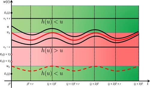
Assume that there exists $u_2\in (u_1,E_1(j+1,c))$ such that $\begin{array}{r}h(u_2)=u_2,\mathrm{and}h(u)>u\mathrm{for}u\in (u_2,E_1(j+1,c)),\end{array}$ see Figure 2(B) and (C) for illustration. Then, the growth rate of the Poincaré map h at $u_i$ with i = 1, 2 satisfies one of the following two conclusions: (27) $\begin{array}{r}(\mathrm{i})h^{\prime }(u_1)\ge 1,h^{\prime }(u_2)=1;(\mathrm{ii})h^{\prime }(u_1)=1,h^{\prime }(u_2)\ge 1,\end{array}$(27) which correspond to Figure 2(B) and (C), respectively.

Figure 2. When $0<c\le G^{\ast }$, schematic illustrations for proving the uniqueness of T-periodic solutions initiated from $(E_1(j),E_1(j+1))$, where $E_1(k)=E_1(k,c),k=j,j+1$. Panel (A) graphs that model (3(3) $\begin{array}{r}\{\begin{array}{l}\begin{array}{rl}\frac{\mathrm{d}w}{\mathrm{d}t}& =-\frac{a\xi w}{w+(j+1)c}[{(w-\frac{A}{2})}^2+\frac{\mu (j+1)}{a\xi }(c-G^{\ast })],t\in [(i-1)T,(i-1)T+r),\\ \frac{\mathrm{d}w}{\mathrm{d}t}& =-\frac{a\xi w}{w+jc}[{(w-\frac{A}{2})}^2+\frac{\mu j}{a\xi }(c-\frac{j+1}{j}{G}^{\ast })],t\in [(i-1)T+r,iT),\end{array}\end{array}\end{array}$(3) ) has a unique T-periodic solution, panels (B) and (C) describe that model (3(3) $\begin{array}{r}\{\begin{array}{l}\begin{array}{rl}\frac{\mathrm{d}w}{\mathrm{d}t}& =-\frac{a\xi w}{w+(j+1)c}[{(w-\frac{A}{2})}^2+\frac{\mu (j+1)}{a\xi }(c-G^{\ast })],t\in [(i-1)T,(i-1)T+r),\\ \frac{\mathrm{d}w}{\mathrm{d}t}& =-\frac{a\xi w}{w+jc}[{(w-\frac{A}{2})}^2+\frac{\mu j}{a\xi }(c-\frac{j+1}{j}{G}^{\ast })],t\in [(i-1)T+r,iT),\end{array}\end{array}\end{array}$(3) ) has exactly two T-periodic solutions, which correspond to cases (i) and (ii) in (27(27) $\begin{array}{r}(\mathrm{i})h^{\prime }(u_1)\ge 1,h^{\prime }(u_2)=1;(\mathrm{ii})h^{\prime }(u_1)=1,h^{\prime }(u_2)\ge 1,\end{array}$(27) ), respectively.

To obtain a contradiction, we need to take the derivative of $h(u)$. Set $\begin{array}{r}M(u,k)=\frac{u+kc}{u(u-E_1(k,c))(u-E_2(k,c))}.\end{array}$ Then we have, from (16(16) $\begin{array}{rl}& \frac{\overline{h}(u)+(j+1)c}{\overline{h}\left(u\right)(\overline{h}\left(u\right)-E_1(j+1,c))(\overline{h}\left(u\right)-E_2(j+1,c))}{\overline{h}}^{\prime }\left(u\right)=\frac{u+(j+1)c}{u(u-E_1(j+1,c))(u-E_2(j+1,c))}.\end{array}$(16) ) and (20(20) $\begin{array}{r}\frac{(h\left(u\right)+jc)h^{\prime }\left(u\right)}{h\left(u\right)(h\left(u\right)-E_1(j,c))(h\left(u\right)-E_2(j,c))}=\frac{(\overline{h}\left(u\right)+jc){\overline{h}}^{\prime }\left(u\right)}{\overline{h}\left(u\right)(\overline{h}\left(u\right)-E_1(j,c))(\overline{h}\left(u\right)-E_2(j,c))}.\end{array}$(20) ), $\begin{array}{r}{\overline{h}}^{\prime }\left(u\right)=\frac{M(u,j+1)}{M(\overline{h}(u),j+1)}\mathrm{and}{h}^{\prime }\left(u\right)=\frac{M(\overline{h}(u),j)}{M(h(u),j)}\cdot \frac{M(u,j+1)}{M(\overline{h}(u),j+1)}.\end{array}$ Define (28) $\begin{array}{r}N\left(u\right)=\frac{M(u,j)}{M(u,j+1)}=\frac{u+jc}{u+(j+1)c}\cdot \frac{u-E_1(j+1,c)}{u-E_1(j,c)}\cdot \frac{u-E_2(j+1,c)}{u-E_2(j,c)}.\end{array}$(28) Then at points $u_i$, we have $h^{\prime }(u_i)=\frac{N(\overline{h}(u_i))}{N(u_i)}$. Since $\begin{array}{r}{E}_1(j,c)<u<E_1(j+1,c)<E_2(j+1,c)<E_2(j,c),\end{array}$ we have $N(u_i)<0,i=1,2$. From (27(27) $\begin{array}{r}(\mathrm{i})h^{\prime }(u_1)\ge 1,h^{\prime }(u_2)=1;(\mathrm{ii})h^{\prime }(u_1)=1,h^{\prime }(u_2)\ge 1,\end{array}$(27) ), cases (i) and (ii) imply (29) $\begin{array}{r}N\left(\overline{h}\left(u_1\right)\right)\le N\left(u_1\right)\mathrm{and}N\left(\overline{h}\left(u_2\right)\right)=N(u_2),\end{array}$(29) and (30) $\begin{array}{r}N\left(\overline{h}\left(u_1\right)\right)=N\left(u_1\right)\mathrm{and}N\left(\overline{h}\left(u_2\right)\right)\le N(u_2),\end{array}$(30) respectively.

However, from (28(28) $\begin{array}{r}N\left(u\right)=\frac{M(u,j)}{M(u,j+1)}=\frac{u+jc}{u+(j+1)c}\cdot \frac{u-E_1(j+1,c)}{u-E_1(j,c)}\cdot \frac{u-E_2(j+1,c)}{u-E_2(j,c)}.\end{array}$(28) ), we have $\begin{array}{r}\begin{array}{rl}\frac{N^{\prime }\left(u\right)}{N\left(u\right)}& =\frac{1}{u+jc}+\frac{1}{u-E_1(j+1,c)}+\frac{1}{u-E_2(j+1,c)}-\frac{1}{u+(j+1)c}\\ & -\frac{1}{u-E_1(j,c)}-\frac{1}{u-E_2(j,c)}\\ & =\frac{1}{u+jc}+\frac{1}{E_2(j,c)-u}-\frac{1}{E_2(j+1,c)-u}-\frac{1}{u+(j+1)c}\\ & -\frac{1}{E_1(j+1,c)-u}-\frac{1}{u-E_1(j,c)}\\ & <\frac{1}{u+jc}+\frac{1}{E_2(j,c)-u}-\frac{1}{E_1(j+1,c)-u}-\frac{1}{u-E_1(j,c)}\\ & =(\frac{1}{u+jc}-\frac{1}{u-E_1(j,c)})-(\frac{1}{E_1(j+1,c)-u}-\frac{1}{E_2(j,c)-u})\\ & <0,\end{array}\end{array}$ which, along with $N(u)<0$ for $u\in (E_1(j,c),E_1(j+1,c))$, yield (31) $\begin{array}{r}{N}^{\prime }\left(u\right)>0\mathrm{for}u\in (E_1(j,c),E_1(j+1,c)).\end{array}$(31) Since $h(u_i)=u_i,\overline{h}(u_i)>E_1(j,c)$ always holds. Otherwise, we have $h(u_i)\le E_1(j,c)<u_i$. Hence, from (31(31) $\begin{array}{r}{N}^{\prime }\left(u\right)>0\mathrm{for}u\in (E_1(j,c),E_1(j+1,c)).\end{array}$(31) ) and the facts $\overline{h}(u_i)<u_i$, we have $N(\overline{h}(u_i))<N(u_i),i=1,2$. A contradiction to (29(29) $\begin{array}{r}N\left(\overline{h}\left(u_1\right)\right)\le N\left(u_1\right)\mathrm{and}N\left(\overline{h}\left(u_2\right)\right)=N(u_2),\end{array}$(29) ) and (30(30) $\begin{array}{r}N\left(\overline{h}\left(u_1\right)\right)=N\left(u_1\right)\mathrm{and}N\left(\overline{h}\left(u_2\right)\right)\le N(u_2),\end{array}$(30) ). Obviously, (31(31) $\begin{array}{r}{N}^{\prime }\left(u\right)>0\mathrm{for}u\in (E_1(j,c),E_1(j+1,c)).\end{array}$(31) ) can also exclude the possibility of three or more T-periodic solutions to model (3(3) $\begin{array}{r}\{\begin{array}{l}\begin{array}{rl}\frac{\mathrm{d}w}{\mathrm{d}t}& =-\frac{a\xi w}{w+(j+1)c}[{(w-\frac{A}{2})}^2+\frac{\mu (j+1)}{a\xi }(c-G^{\ast })],t\in [(i-1)T,(i-1)T+r),\\ \frac{\mathrm{d}w}{\mathrm{d}t}& =-\frac{a\xi w}{w+jc}[{(w-\frac{A}{2})}^2+\frac{\mu j}{a\xi }(c-\frac{j+1}{j}{G}^{\ast })],t\in [(i-1)T+r,iT),\end{array}\end{array}\end{array}$(3) ). The proof is complete.

Lemma 3.3

Assume that $0<c\le G^{\ast }$. Then model (3(3) $\begin{array}{r}\{\begin{array}{l}\begin{array}{rl}\frac{\mathrm{d}w}{\mathrm{d}t}& =-\frac{a\xi w}{w+(j+1)c}[{(w-\frac{A}{2})}^2+\frac{\mu (j+1)}{a\xi }(c-G^{\ast })],t\in [(i-1)T,(i-1)T+r),\\ \frac{\mathrm{d}w}{\mathrm{d}t}& =-\frac{a\xi w}{w+jc}[{(w-\frac{A}{2})}^2+\frac{\mu j}{a\xi }(c-\frac{j+1}{j}{G}^{\ast })],t\in [(i-1)T+r,iT),\end{array}\end{array}\end{array}$(3) ) has a unique T-periodic solution $w(t;jT,v_1)$ with $v_1\in (E_2(j+1,c),E_2(j,c))$.

Proof.

From Lemma 3.1, there exists $v_1\in (E_2(j+1,c),E_2(j,c))$ such that $\begin{array}{r}h(v_1)=v_1,h^{\prime }(v_1)\le 1,\mathrm{and}h(u)>u\mathrm{for}u\in (E_2(j+1,c),v_1).\end{array}$ Denote $w_2(t)=w(t;jT,v_1)$. Then $w_2(t)>w_1(t)$, and $w_2(t)$ is a T-periodic solution of model (3(3) $\begin{array}{r}\{\begin{array}{l}\begin{array}{rl}\frac{\mathrm{d}w}{\mathrm{d}t}& =-\frac{a\xi w}{w+(j+1)c}[{(w-\frac{A}{2})}^2+\frac{\mu (j+1)}{a\xi }(c-G^{\ast })],t\in [(i-1)T,(i-1)T+r),\\ \frac{\mathrm{d}w}{\mathrm{d}t}& =-\frac{a\xi w}{w+jc}[{(w-\frac{A}{2})}^2+\frac{\mu j}{a\xi }(c-\frac{j+1}{j}{G}^{\ast })],t\in [(i-1)T+r,iT),\end{array}\end{array}\end{array}$(3) ). Hence, we only need to prove the uniqueness of T-periodic solutions to model (3(3) $\begin{array}{r}\{\begin{array}{l}\begin{array}{rl}\frac{\mathrm{d}w}{\mathrm{d}t}& =-\frac{a\xi w}{w+(j+1)c}[{(w-\frac{A}{2})}^2+\frac{\mu (j+1)}{a\xi }(c-G^{\ast })],t\in [(i-1)T,(i-1)T+r),\\ \frac{\mathrm{d}w}{\mathrm{d}t}& =-\frac{a\xi w}{w+jc}[{(w-\frac{A}{2})}^2+\frac{\mu j}{a\xi }(c-\frac{j+1}{j}{G}^{\ast })],t\in [(i-1)T+r,iT),\end{array}\end{array}\end{array}$(3) ) for $u\in (E_2(j+1,c),E_2(j,c))$. Similarly, assume that model (3(3) $\begin{array}{r}\{\begin{array}{l}\begin{array}{rl}\frac{\mathrm{d}w}{\mathrm{d}t}& =-\frac{a\xi w}{w+(j+1)c}[{(w-\frac{A}{2})}^2+\frac{\mu (j+1)}{a\xi }(c-G^{\ast })],t\in [(i-1)T,(i-1)T+r),\\ \frac{\mathrm{d}w}{\mathrm{d}t}& =-\frac{a\xi w}{w+jc}[{(w-\frac{A}{2})}^2+\frac{\mu j}{a\xi }(c-\frac{j+1}{j}{G}^{\ast })],t\in [(i-1)T+r,iT),\end{array}\end{array}\end{array}$(3) ) has another T-periodic solution in this case, and we denote it by $w(t;jT,v_2)$. Then as illustrated in Figure 3(A) and (B), there are two cases: (32) $\begin{array}{r}(\mathrm{i})h^{\prime }(v_1)\le 1,h^{\prime }(v_2)=1;(\mathrm{ii})h^{\prime }(v_1)=1,h^{\prime }(v_2)\le 1,\end{array}$(32) and $\begin{array}{r}h(u)<u\mathrm{for}u\in (v_2,E_2(j,c)).\end{array}$ Meanwhile, the facts $h^{\prime }(v_i)=\frac{N(\overline{h}(v_i))}{N(v_i)}\le 1$ with i = 1, 2 and $N(u)<0$ for $u\in (E_2(j+1,c),E_2(j,c))$ imply (33) $\begin{array}{r}N\left(\overline{h}\left(v_1\right)\right)\ge N(v_1),N\left(\overline{h}\left(v_2\right)\right)=N(v_2),\end{array}$(33) and (34) $\begin{array}{r}N\left(\overline{h}\left(v_1\right)\right)=N(v_1),N\left(\overline{h}\left(v_2\right)\right)\ge N(v_2)\end{array}$(34) hold, which respectively correspond to cases (i) and (ii) in (32(32) $\begin{array}{r}(\mathrm{i})h^{\prime }(v_1)\le 1,h^{\prime }(v_2)=1;(\mathrm{ii})h^{\prime }(v_1)=1,h^{\prime }(v_2)\le 1,\end{array}$(32) ).

Figure 3. When $0<c\le G^{\ast }$, schematic illustrations for proving the uniqueness of T-periodic solutions initiated from $(E_2(j+1),E_2(j))$, where $E_2(k)=E_2(k,c),k=j,j+1$. Panels (A) and (B) manifest that model (3(3) $\begin{array}{r}\{\begin{array}{l}\begin{array}{rl}\frac{\mathrm{d}w}{\mathrm{d}t}& =-\frac{a\xi w}{w+(j+1)c}[{(w-\frac{A}{2})}^2+\frac{\mu (j+1)}{a\xi }(c-G^{\ast })],t\in [(i-1)T,(i-1)T+r),\\ \frac{\mathrm{d}w}{\mathrm{d}t}& =-\frac{a\xi w}{w+jc}[{(w-\frac{A}{2})}^2+\frac{\mu j}{a\xi }(c-\frac{j+1}{j}{G}^{\ast })],t\in [(i-1)T+r,iT),\end{array}\end{array}\end{array}$(3) ) has exactly two T-periodic solutions, which correspond to cases (i) and (ii) in (32(32) $\begin{array}{r}(\mathrm{i})h^{\prime }(v_1)\le 1,h^{\prime }(v_2)=1;(\mathrm{ii})h^{\prime }(v_1)=1,h^{\prime }(v_2)\le 1,\end{array}$(32) ), respectively.

However, taking the derivative of $N(u)$ yields $\begin{array}{r}\begin{array}{rl}\frac{N^{\prime }\left(u\right)}{N\left(u\right)}& =\frac{1}{u+jc}+\frac{1}{E_2(j,c)-u}+\frac{1}{u-E_2(j+1,c)}+\frac{1}{u-E_1(j+1,c)}\\ & -\frac{1}{u+(j+1)c}-\frac{1}{u-E_1(j,c)}\\ & >\frac{1}{u+jc}-\frac{1}{u+(j+1)c}+\frac{1}{u-E_2(j+1,c)}-\frac{1}{u-E_1(j,c)}\\ & >0,\end{array}\end{array}$ and hence $N^{\prime }(u)<0$ for $u\in (E_2(j+1,c),E_2(j,c))$, which leads to a contradiction to $N(\overline{h}(v_2))=N(v_2)$ in (33(33) $\begin{array}{r}N\left(\overline{h}\left(v_1\right)\right)\ge N(v_1),N\left(\overline{h}\left(v_2\right)\right)=N(v_2),\end{array}$(33) ) and a contradiction to $N(\overline{h}(v_1))=N(v_1)$ in (34(34) $\begin{array}{r}N\left(\overline{h}\left(v_1\right)\right)=N(v_1),N\left(\overline{h}\left(v_2\right)\right)\ge N(v_2)\end{array}$(34) ). Further, $N^{\prime }(u)<0$ is sufficient to exclude the possibility of three or more T-periodic solutions to model (3(3) $\begin{array}{r}\{\begin{array}{l}\begin{array}{rl}\frac{\mathrm{d}w}{\mathrm{d}t}& =-\frac{a\xi w}{w+(j+1)c}[{(w-\frac{A}{2})}^2+\frac{\mu (j+1)}{a\xi }(c-G^{\ast })],t\in [(i-1)T,(i-1)T+r),\\ \frac{\mathrm{d}w}{\mathrm{d}t}& =-\frac{a\xi w}{w+jc}[{(w-\frac{A}{2})}^2+\frac{\mu j}{a\xi }(c-\frac{j+1}{j}{G}^{\ast })],t\in [(i-1)T+r,iT),\end{array}\end{array}\end{array}$(3) ). We complete the proof.

With the above three lemmas, we are now ready to give the detailed proof of the theorem.

Proof

Proof of the Theorem

From Lemmas 3.1–3.3, we have already known that model (3(3) $\begin{array}{r}\{\begin{array}{l}\begin{array}{rl}\frac{\mathrm{d}w}{\mathrm{d}t}& =-\frac{a\xi w}{w+(j+1)c}[{(w-\frac{A}{2})}^2+\frac{\mu (j+1)}{a\xi }(c-G^{\ast })],t\in [(i-1)T,(i-1)T+r),\\ \frac{\mathrm{d}w}{\mathrm{d}t}& =-\frac{a\xi w}{w+jc}[{(w-\frac{A}{2})}^2+\frac{\mu j}{a\xi }(c-\frac{j+1}{j}{G}^{\ast })],t\in [(i-1)T+r,iT),\end{array}\end{array}\end{array}$(3) ) has exactly two T-periodic solutions, namely, $w_1(t)$ and $w_2(t)$, and (35) $\begin{array}{r}h(u)<u\mathrm{for}u\in (0,u_1)\cup (v_1,+\mathrm{\infty }),h(u)>u\mathrm{for}u\in (u_1,v_1),\end{array}$(35) as shown in Figure 4. Let ${\delta }_0=u_1$, then from Lemma 2.2 and (35(35) $\begin{array}{r}h(u)<u\mathrm{for}u\in (0,u_1)\cup (v_1,+\mathrm{\infty }),h(u)>u\mathrm{for}u\in (u_1,v_1),\end{array}$(35) ), we obtain that $w_1(t)$ is unstable. Hence, we only need to prove that $w_2(t)$ is asymptotically stable.

Figure 4. A schematic illustration for figuring out the proof of the asymptotic stability to the larger T-periodic solution $w_2(t)$, which is the solid red curve, where $E_i(k)=E_i(k,c),i=1,2,k=j,j+1$.

For convenience, we denote $w(t)=w(t;t_0,u_0)$ in the following.

We first prove that $w_2(t)$ is stable. For any $\epsilon \in (0,min\{v_1-E_2(j+1,c),E_2(j,c)-v_1\})$, we only need to show that $|u_0-w_2(t_0)|<\delta$ implies (36) $\begin{array}{r}|w(t;t_0,u_0)-w_2\left(t\right)|<\epsilon ,\mathrm{for}t\ge t_0,\end{array}$(36) where $\delta =\delta (\epsilon ,t_0)>0$. To this end, we choose $\delta =\epsilon$, and prove (36(36) $\begin{array}{r}|w(t;t_0,u_0)-w_2\left(t\right)|<\epsilon ,\mathrm{for}t\ge t_0,\end{array}$(36) ) by contradiction. In fact, if not, then there exists $\overline{t}>t_0$ such that $\begin{array}{r}|w(t;t_0,u_0)-w_2\left(t\right)|<\epsilon \mathrm{for}t\in [t_0,\overline{t}),\mathrm{and}|w(\overline{t};t_0,u_0)-w_2\left(\overline{t}\right)|=\epsilon .\end{array}$ Without loss of generality, we assume that $\begin{array}{r}w(t;t_0,u_0)>w_2\left(t\right)-\epsilon \mathrm{for}t\in [t_0,\overline{t}),\mathrm{and}w(\overline{t};t_0,u_0)=w_2\left(\overline{t}\right)-\epsilon .\end{array}$ Since (3(3) $\begin{array}{r}\{\begin{array}{l}\begin{array}{rl}\frac{\mathrm{d}w}{\mathrm{d}t}& =-\frac{a\xi w}{w+(j+1)c}[{(w-\frac{A}{2})}^2+\frac{\mu (j+1)}{a\xi }(c-G^{\ast })],t\in [(i-1)T,(i-1)T+r),\\ \frac{\mathrm{d}w}{\mathrm{d}t}& =-\frac{a\xi w}{w+jc}[{(w-\frac{A}{2})}^2+\frac{\mu j}{a\xi }(c-\frac{j+1}{j}{G}^{\ast })],t\in [(i-1)T+r,iT),\end{array}\end{array}\end{array}$(3) ) is T-periodic, we may assume $t_0\in [(j+1)T,(j+2)T)$.

Let i>j be a positive integer such that $\overline{t}\in (iT,(i+1)T]$. Then there are three possible cases to consider: (I) $\overline{t}=(i+1)T$; (II) $\overline{t}=iT+r$; (III) $\overline{t}\in (iT,iT+r)\cup (iT+r,(i+1)T)$. We first show that (I) is impossible. In fact, if (I) holds, then we have $\begin{array}{r}{h}_{i+1}\left(u_0\right)=h_{i+1}\left(v_1\right)-\epsilon ,\mathrm{and}{h}_n\left(u_0\right)>h_n\left(v_1\right)-\epsilon \mathrm{for}n=0,1,2,\dots ,i,\end{array}$ which shows that $\begin{array}{r}{h}_{i+1}\left(u_0\right)=h_{i+1}\left(v_1\right)-\epsilon =h_i\left(v_1\right)-\epsilon <h_i(u_0).\end{array}$ However, from Lemmas 2.1, 3.1–3.3, we know that sequence $\{h_n(u_0)\}$ is strictly increasing, which leads to a contradiction. Thus, (I) is impossible.

We then prove that (II) is also impossible. If not, then we have (37) $\begin{array}{r}w\left(t\right)>w_2\left(t\right)-\epsilon \mathrm{for}t\in [t_0,iT+r),\mathrm{and}w(iT+r)=w_2(iT+r)-\epsilon .\end{array}$(37) Furthermore, from (12(12) $\begin{array}{r}{L}_1(u,k)=u^{{\alpha }_1(k)}\cdot {|u-E_1(k,c)|}^{{\beta }_1(k)}\cdot {|u-E_2(k,c)|}^{{\gamma }_1(k)}.\end{array}$(12) ) and (13(13) $\begin{array}{r}\frac{\mathrm{\partial }{L}_1(u,k)}{\mathrm{\partial }u}=L_1(u,k)\frac{u+kc}{u(u-E_1(k,c))(u-E_2(k,c))}.\end{array}$(13) ), with k = j, we can derive that $\begin{array}{r}{L}_1(u,j)>0,\mathrm{and}\frac{\mathrm{\partial }{L}_1(u,j)}{\mathrm{\partial }u}<0,\mathrm{for}u\in (E_2(j+1,c),E_2(j,c)),\end{array}$ which manifests that function $L_1(u,j)$ is strictly decreasing with respect to u. Thus, from (18(18) $\begin{array}{r}{L}_1(h\left(u\right),j)=L_1(\overline{h}\left(u\right),j)e^{-a\xi (T-r)}.\end{array}$(18) ) and (37(37) $\begin{array}{r}w\left(t\right)>w_2\left(t\right)-\epsilon \mathrm{for}t\in [t_0,iT+r),\mathrm{and}w(iT+r)=w_2(iT+r)-\epsilon .\end{array}$(37) ), we have $\begin{array}{r}\begin{array}{rl}{L}_1(w\left((i+1)T\right),j)& =L_1(w(iT+r),j)e^{-a\xi (T-r)}\\ & =L_1(w_2(iT+r)-\epsilon ,j)e^{-a\xi (T-r)}\\ & =L_1(w_2((i-1)T+r)-\epsilon ,j)e^{-a\xi (T-r)}\\ & >L_1(w((i-1)T+r),j)e^{-a\xi (T-r)}\\ & =L_1(w\left(iT\right),j),\end{array}\end{array}$ that is, we have $w((i+1)T)<w(iT)$, or, equivalently, $h_{i+1}(u_0)<h_i(u_0)$, which gives a similar contradiction to that in the proof of case (I). Thus, (II) is also impossible.

Finally, we prove (III) is impossible as well. We first prove that the case of $\overline{t}\in (iT,iT+r)$ is impossible. Integrating (9(9) $\begin{array}{r}\mathrm{d}[\ln (w^{{\alpha }_1(k)}\cdot {|w-E_1(k,c)|}^{{\beta }_1(k)}\cdot {|w-E_2(k,c)|}^{{\gamma }_1(k)})]=-a\xi \mathrm{d}t.\end{array}$(9) ) from iT to $\overline{t}$ with k = j + 1, we obtain (38) $\begin{array}{r}{L}_1(w\left(\overline{t}\right),j+1)=L_1(w\left(iT\right),j+1)e^{-a\xi (\overline{t}-iT)},\end{array}$(38) similarly, integrating (9(9) $\begin{array}{r}\mathrm{d}[\ln (w^{{\alpha }_1(k)}\cdot {|w-E_1(k,c)|}^{{\beta }_1(k)}\cdot {|w-E_2(k,c)|}^{{\gamma }_1(k)})]=-a\xi \mathrm{d}t.\end{array}$(9) ) from $(i-1)T$ to $\overline{t}-T$ with k = j + 1, we get (39) $\begin{array}{r}{L}_1(w(\overline{t}-T),j+1)=L_1(w\left((i-1)T\right),j+1)e^{-a\xi (\overline{t}-iT)},\end{array}$(39) from (12(12) $\begin{array}{r}{L}_1(u,k)=u^{{\alpha }_1(k)}\cdot {|u-E_1(k,c)|}^{{\beta }_1(k)}\cdot {|u-E_2(k,c)|}^{{\gamma }_1(k)}.\end{array}$(12) ) and (13(13) $\begin{array}{r}\frac{\mathrm{\partial }{L}_1(u,k)}{\mathrm{\partial }u}=L_1(u,k)\frac{u+kc}{u(u-E_1(k,c))(u-E_2(k,c))}.\end{array}$(13) ), with k = j + 1, we have $\begin{array}{r}{L}_1(u,j+1)>0,\mathrm{and}\frac{\mathrm{\partial }{L}_1(u,j+1)}{\mathrm{\partial }u}>0,\mathrm{for}u\in (E_2(j+1,c),E_2(j,c)),\end{array}$ which implies that function $L_1(u,j+1)$ is strictly increasing with respect to u. Furthermore, since (40) $\begin{array}{r}w\left(\overline{t}\right)=w_2\left(\overline{t}\right)-\epsilon =w_2(\overline{t}-T)-\epsilon <w(\overline{t}-T),\end{array}$(40) (38(38) $\begin{array}{r}{L}_1(w\left(\overline{t}\right),j+1)=L_1(w\left(iT\right),j+1)e^{-a\xi (\overline{t}-iT)},\end{array}$(38) ) and (39(39) $\begin{array}{r}{L}_1(w(\overline{t}-T),j+1)=L_1(w\left((i-1)T\right),j+1)e^{-a\xi (\overline{t}-iT)},\end{array}$(39) ) tell us that $L_1(w(iT),j+1)<L_1(w((i-1)T),j+1)$, therefore, follows from the increasing monotonicity of $L_1(u,j+1)$ with respect to u, we have $w(iT)<w((i-1)T)$, a similar contradiction to that in the proof of case (I) occurs again. Thus, the case of $\overline{t}\in (iT,iT+r)$ is impossible.

We then prove the case of $\overline{t}\in (iT+r,(i+1)T)$ is also impossible. Integrating (9(9) $\begin{array}{r}\mathrm{d}[\ln (w^{{\alpha }_1(k)}\cdot {|w-E_1(k,c)|}^{{\beta }_1(k)}\cdot {|w-E_2(k,c)|}^{{\gamma }_1(k)})]=-a\xi \mathrm{d}t.\end{array}$(9) ) from $\overline{t}$ to $(i+1)T$ with k = j, we have (41) $\begin{array}{r}{L}_1(w\left((i+1)T\right),j)=L_1(w\left(\overline{t}\right),j)e^{-a\xi ((i+1)T-\overline{t})}.\end{array}$(41) Similarly, integrating (9(9) $\begin{array}{r}\mathrm{d}[\ln (w^{{\alpha }_1(k)}\cdot {|w-E_1(k,c)|}^{{\beta }_1(k)}\cdot {|w-E_2(k,c)|}^{{\gamma }_1(k)})]=-a\xi \mathrm{d}t.\end{array}$(9) ) from $\overline{t}-T$ to iT with k = j, we reach (42) $\begin{array}{r}{L}_1(w\left(iT\right),j)=L_1(w(\overline{t}-T),j)e^{-a\xi ((i+1)T-\overline{t})}.\end{array}$(42) Recall that function $L_1(u,j)$ is strictly decreasing with respect to u, thus, (40(40) $\begin{array}{r}w\left(\overline{t}\right)=w_2\left(\overline{t}\right)-\epsilon =w_2(\overline{t}-T)-\epsilon <w(\overline{t}-T),\end{array}$(40) ), (41(41) $\begin{array}{r}{L}_1(w\left((i+1)T\right),j)=L_1(w\left(\overline{t}\right),j)e^{-a\xi ((i+1)T-\overline{t})}.\end{array}$(41) ) and (42(42) $\begin{array}{r}{L}_1(w\left(iT\right),j)=L_1(w(\overline{t}-T),j)e^{-a\xi ((i+1)T-\overline{t})}.\end{array}$(42) ) give $L_1(w((i+1)T),j)>L_1(w(iT),j)$, hence, we obtain $w((i+1)T)<w(iT)$. A similar contradiction as that in the proof of case (I) can be achieved. Thus, the case of $\overline{t}\in (iT+r,(i+1)T)$ is also impossible. Hence, (36(36) $\begin{array}{r}|w(t;t_0,u_0)-w_2\left(t\right)|<\epsilon ,\mathrm{for}t\ge t_0,\end{array}$(36) ) is true, which implies that $w_2(t)$ is stable.

For the attractivity of $w_2(t)$, we need to prove (43) $\begin{array}{r}\underset{t\to \mathrm{\infty }}{lim}[w(t;t_0,u_0)-w_2\left(t\right)]=0,\mathrm{for}\mathrm{any}{u}_0>u_1.\end{array}$(43) For the case when $u_0\in (u_1,v_1)$, from (35(35) $\begin{array}{r}h(u)<u\mathrm{for}u\in (0,u_1)\cup (v_1,+\mathrm{\infty }),h(u)>u\mathrm{for}u\in (u_1,v_1),\end{array}$(35) ), we have $h(u_0)>u_0$, hence, $\underset{n\to \mathrm{\infty }}{lim}w(nT;t_0,u_0)=v_1$. In fact, from Lemma 2.1, we know that sequence $\{w(nT;t_0,u_0)\}$ is strictly increasing, so $\begin{array}{r}\underset{t\to \mathrm{\infty }}{lim}w(t;t_0,u_0)=\underset{n\to \mathrm{\infty }}{lim}w(nT;t_0,u_0)=v_1,\end{array}$ this shows that (43(43) $\begin{array}{r}\underset{t\to \mathrm{\infty }}{lim}[w(t;t_0,u_0)-w_2\left(t\right)]=0,\mathrm{for}\mathrm{any}{u}_0>u_1.\end{array}$(43) ) is true for the case when $u_0\in (u_1,v_1)$. For the case when $u_0\in (v_1,+\mathrm{\infty })$, from (35(35) $\begin{array}{r}h(u)<u\mathrm{for}u\in (0,u_1)\cup (v_1,+\mathrm{\infty }),h(u)>u\mathrm{for}u\in (u_1,v_1),\end{array}$(35) ), we have $h(u_0)<u_0$, the remaining proof is similar to that of $u_0\in (u_1,v_1)$ and is omitted. We complete the proof.

In the following, we will carry out a numerical example to illustrate our theoretical results.

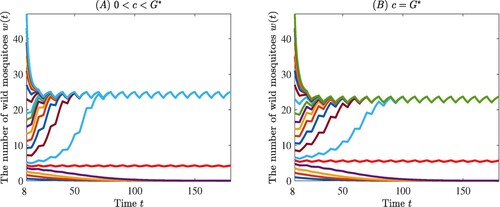
Example 1

Let $\begin{array}{r}a=35.05,\mu =0.05,\xi =0.035,\mathrm{and}\overline{T}=14.\end{array}$ By taking $T=10<\overline{T}$, we have $G^{\ast }=2496.4$. Then we choose $c=2000<G^{\ast }$ or $c=2496.4=G^{\ast }$, the condition of the Theorem is satisfied and $w_0$ is asymptotically stable, along with an asymptotically stable T-periodic solution, which are respectively shown in panels (A) and (B) of Figure 5.

Figure 5. Panels (A) and (B) are used to support our theoretical results, where the two curves in red colour represent the unstable T-periodic solution $w_1(t)$.

4. Concluding remarks

Based on the modelling idea in [31] that the number of sterile mosquitoes released is treated as a given nonnegative function rather than a variable satisfying an independent dynamical equation, the interactive dynamics of wild and sterile mosquitoes with or without time delay has been recently studied in [18,21,32–34,41]. A common assumption is that the sterile mosquitoes are impulsively and periodically released at discrete time points kT, $k=0,1,2,\dots$. Such impulsive and periodic release strategy is consistent with the actual field release situation [42].

Model (1(1) $\begin{array}{r}\frac{\mathrm{d}w}{\mathrm{d}t}=\frac{a{w}^2(1-\xi w)}{w+g}-\mu w,\end{array}$(1) ) is derived by combining the ideas in [6] and [31]. We introduce two release amount thresholds $g^{\ast }$ and $c^{\ast }$, and the waiting period threshold $T^{\ast }$. In [43], for the case of $c\ge c^{\ast }$, the authors obtained sufficient conditions for the global asymptotic stability of the origin and the existence of a globally asymptotically stable T-periodic solution, respectively. It is well known for obtaining sufficient conditions on the existence of exact two periodic solutions is mathematically challenging. In this paper, for the case of $c\in (0,G^{\ast }]$, we show that model (1(1) $\begin{array}{r}\frac{\mathrm{d}w}{\mathrm{d}t}=\frac{a{w}^2(1-\xi w)}{w+g}-\mu w,\end{array}$(1) ) has exactly two T-periodic solutions and analyse their stability, the bigger one is stable and the smaller one is unstable. The result, combining with that of [43], indicates the better understanding of how to determine a better release strategy for biological control of wild mosquitoes from practical release perspective. Further investigations, for the case of $G^{\ast }<c<G^{\ast \ast }$, are understudy, this will be a topic of our future study. We hope that our theoretical results can provide real guidance to help the practical workers make the better release strategy to gain a better effect for the wild mosquito population suppression.

Disclosure statement

No potential conflict of interest was reported by the author(s).

Additional information

Funding

This work is supported by National Natural Science Foundation of China [grant numbers 12071095, 12026222, 12026236] and Innovative Research Grant for the Postgraduates of Guangzhou University [grant number 2019GDJC-D05].

References

- S. Ai, J. Li, J. Yu and B. Zheng, Stage-structured models for interactive wild and periodically and impulsively released sterile mosquitoes, Discrete Contin. Dyn. Syst. Ser. B, doi: 10.3934/dcdsb.2021172.
- L. Alphey, M. Benedict and R. Bellini, et al. Sterile-insect methods for control of mosquito-borne diseases: An analysis, Vector Borne Zoonotic Dis. 10 (2010), pp. 295–311.
- H. Barclay, Pest population stability under sterile releases, Res. Popul. Ecol. 24 (1982), pp. 405–416.
- H. Barclay, Mathematical models for the use of sterile insects, In: Sterile insect technique: Principles and practice in area-wide integrated pest management, V. Dyck, J. Hendrichs and A. Robinson, eds., Springer, Netherlands, 2005, pp. 147–174.
- L. Cai, S. Ai and G. Fan, Dynamics of delayed mosquitoes populations models with two different strategies of releasing sterile mosquitoes, Math. Biosci. Eng. 15 (2018), pp. 1181–1202.
- L. Cai, S. Ai and J. Li, Dynamics of mosquitoes populations with different strategies for releasing sterile mosquitoes, SIAM J. Appl. Math. 74 (2014), pp. 1786–1809.
- CDC, Life cycle: The mosquito, Preprint 2019, Available from: https://www.cdc.gov/dengue/resources/factsheets/mosquitolifecyclefinal.pdf.
- K. Fister, M. McCarthy, S. Oppenheimer and C. Collins, Optimal control of insects through sterile insect release and habitat modification, Math. Biosci. 244 (2013), pp. 201–212.
- Z. Guo, H. Guo and Y. Chen, Traveling wavefronts of a delayed temporally discrete reaction-diffusion equation, J. Math. Anal. Appl. 496 (2021), pp. 124787.
- M. Hirsch, S. Smale and R. Devaney, Differential Equations, Dynamical Systems, and an Introduction to Chaos, 2nd ed., Academic Press, Orlando, 2003.
- A. Hoffmann, B. Montgomery and J. Popovici, et al. Successful establishment of Wolbachia in Aedes populations to suppress dengue transmission, Nature 476 (2011), pp. 454–457.
- L. Hu, M. Huang, M. Tang, J. Yu and B. Zheng, Wolbachia spread dynamics in stochastic environments, Theor. Popul. Biol. 106 (2015), pp. 32–44.
- L. Hu, M. Tang, Z. Wu, Z. Xi and J. Yu, The threshold infection level for wolbachia invasion in random environment, J. Differ. Equ. 266 (2019), pp. 4377–4393.
- M. Huang, J. Luo, L. Hu, B. Zheng and J. Yu, Assessing the efficiency of Wolbachia driven Aedes mosquito suppression by delay differential equations, J. Theoret. Biol. 440 (2018), pp. 1–11.
- M. Huang, M. Tang and J. Yu, Wolbachia infection dynamics by recation-diffusion equations, Sci. China Math 58 (2015), pp. 77–96.
- M. Huang, M. Tang, J. Yu and B. Zheng, A stage structured model of delay differential equations for Aedes mosquito population suppression, Discrete Contin. Dyn. Syst. 40 (2020), pp. 3467–3484.
- M. Huang, J. Yu, L. Hu and B. Zheng, Qualitative analysis for a Wolbachia infection model with diffusion, Sci. China Math. 59 (2016), pp. 1249–1266.
- Y. Hui, G. Lin, J. Yu and J. Li, A delayed differential equation model for mosquito population suppression with sterile mosquitoes, Discrete Contin. Dyn. Syst. Ser. B 25 (2020), pp. 4659–4676.
- I. Iturbe-Ormaetxe, T. Walker and S. O'Neill. Wolbachia and the biological control of mosquito-borne disease, EMBO Rep. 12 (2011), pp. 508–518.
- J. Li, New revised simple models for interactive wild and sterile mosquito populations and their dynamics, J. Biol. Dyn. 11 (2017), pp. 316–333.
- G. Lin and Y. Hui, Stability analysis in a mosquito population suppression model, J. Biol. Dyn. 14 (2020), pp. 578–589.
- Y. Liu, Z. Guo, M. Smaily and L. Wang, A Wolbachia infection model with free boundary, J. Biol. Dyn. 14 (2020), pp. 515–542.
- Y. Liu, F. Jiao and L. Hu, Modeling mosquito population control by a coupled system, J. Math. Anal. Appl. 506 (2022), pp. 125671.
- F. Liu, C. Yao, P. Lin and C. Zhou, Studies on life table of the natural population of Aedes albopictus, Acta Sci. Nat. Univ. Sunyat. 31 (1992), pp. 84–93.
- Y. Shi and J. Yu, Wolbachia infection enhancing and decaying domains in mosquito population based on discrete models, J. Biol. Dyn. 14 (2020), pp. 679–695.
- Y. Shi and B. Zheng, Discrete dynamical models on Wolbachia infection frequency in mosquito populations with biased release ratios, J. Biol. Dyn., 2021, doi: 10.1080/17513758.2021.1977400.
- C. Stone, Transient population dynamics of mosquitoes during sterile male releases: Modelling mating behaviour and perturbations of life history parameters, PLoS ONE 8 (2013), pp. e76228. doi: 10.1371/journal.pone.0076228.
- E. Waltz, US reviews plan to infect mosquitoes with bacteria to stop disease, Nature 533 (2016), pp. 450–451.
- S. White, P. Rohani and S. Sait, Modelling pulsed releases for sterile insect techniques: Fitness costs of sterile and transgenic males and the effects on mosquito dynamics, J. Appl. Ecol. 47 (2010), pp. 1329–1339.
- World Health Organization, Dengue and severe dengue, Preprint 2021, Available from: http://www.who.int/news-room/fact-sheets/detail/dengue-and-severe-dengue.
- J. Yu, Modelling mosquito population suppression based on delay differential equations, SIAM J. Appl. Math. 78 (2018), pp. 3168–3187.
- J. Yu, Existence and stability of a unique and exact two periodic orbits for an interactive wild and sterile mosquito model, J. Differ. Equ. 269 (2020), pp. 10395–10415.
- J. Yu and J. Li, Dynamics of interactive wild and sterile mosquitoes with time delay, J. Biol. Dyn. 13 (2019), pp. 606–620.
- J. Yu and J. Li, Global asymptotic stability in an interactive wild and sterile mosquito model, J. Differ. Equ. 269 (2020), pp. 6193–6215.
- J. Yu and B. Zheng, Modeling Wolbachia infection in mosquito population via discrete dynamical models, J. Differ. Equ. Appl. 25 (2019), pp. 1549–1567.
- B. Zheng, J. Li and J. Yu, One discrete dynamical model on Wolbachia infection frequency in mosquito populations, Sci. China Math., (2021), doi: 10.1007/s11425-021-1891-7.
- B. Zheng, M. Tang and J. Yu, Modeling Wolbachia spread in mosquitoes through delay differential equation, SIAM J. Appl. Math. 74 (2014), pp. 743–770.
- B. Zheng, M. Tang, J. Yu and J. Qiu, Wolbachia spreading dynamics in mosquitoes with imperfect maternal transmission, J. Math. Biol. 76 (2018), pp. 235–263.
- B. Zheng and J. Yu, Characterization of Wolbachia enhancing domain in mosquitoes with imperfect maternal transmission, J. Biol. Dyn. 12 (2018), pp. 596–610.
- B. Zheng and J. Yu, Existence and uniqueness of periodic orbits in a discrete model on Wolbachia infection frequency, Adv. Nonlinear Anal. 11 (2021), pp. 212–224.
- B. Zheng, J. Yu and J. Li, Modeling and analysis of the implementation of the Wolbachia incompatible and sterile insect technique for mosquito population suppression, SIAM J. Appl. Math. 81 (2021), pp. 718–740.
- X. Zheng, D. Zhang and Y. Li, et al. Incompatible and sterile insect techniques combined eliminate mosquitoes, Nature 572 (2019), pp. 56–61.
- Z. Zhu, B. Zheng, Y. Shi, R. Yan and J. Yu, Stability and periodicity in a mosquito population suppression model composed of two sub-models, Accepted.