Digital thermal monitoring of the Amazon forest: an intercomparison of satellite and reanalysis products

Abstract

Remote sensing and climate digital products have become increasingly available in recent years. Access to these products has favored a variety of Digital Earth studies, such as the analysis of the impact of global warming over different biomes. The study of the Amazon forest response to drought has recently received particular attention from the scientific community due to the occurrence of extreme droughts and anomalous warming over the last decade. This paper focuses on the differences observed between surface thermal anomalies obtained from remote sensing moderate resolution imaging spectroradiometer (MODIS) and climatic (ERA-Interim) monthly products over the Amazon forest. With a few exceptions, results show that the spatial pattern of standardized anomalies is similar for both products. In terms of absolute anomalies, the differences between the two products show a bias near to zero with a standard deviation of around 0.2 K, although the differences can be up to 1 K over particular regions and months. Despite this general agreement, the proper filtering of MODIS daily values in order to construct a new monthly product showed a dramatic reduction in the number of reliable pixels during the rainy season, while for the dry season this reduction is only seen in Northern Amazonia.

Keywords:

• Thermal anomalies
• Amazon forest
• MODIS
• ERA interim
• thermal Amazonia

1. Introduction

Rainforests play an important role in the water and carbon cycles because they store rainwater and absorb atmospheric carbon dioxide. Water is partly released back into the atmosphere through different processes, whereas its capability for absorbing CO₂ might be reduced under different environmental conditions. In particular, the Amazon forests include more than 50% of the world's tropical forests and store more than 100 billion tons of carbon (Malhi et al. 2006), making them a key component of the global carbon cycle. In a global warming scenario, monitoring changes in the Amazon rainforest is critical to understanding its sensitivity to anomalous high temperatures and its impact on forest production. This analysis can be performed over any number of variables, but vegetation/air temperature is one of the key variables linked to plant physiology. For example, some studies found a correlation between a decrease in tropical forest productivity and an increase in temperature, thus reducing its capability for carbon uptake and favoring the accumulation of atmospheric CO₂ (e.g. Clark et al. 2003; Doughty and Goulden 2008).

Variations on temperature are also related to the occurrence of such extreme events as droughts. Indeed, the occurrence of drought events is one major aspect of Amazonian climate change (Malhi et al. 2008). Special attention was paid to Amazonia because of two major droughts, one in 2005 (Marengo et al. 2008) and the other in 2010 (Lewis et al. 2011), both of which were considered amongst the most severe in a century over such a short time span. These drought events have been associated with increased tree mortality and losses in biomass, as well as a temporary shutdown of the Amazon carbon sink (Phillips et al. 2009; Toomey et al. 2011; Saatchi et al. 2013; Gatti et al. 2014).

Analysis of Land Surface Temperature (LST) anomalies from remote sensing and climatic data revealed a significant and sustained warming over this last decade, especially in 2005 and 2010, in the areas where the drought events took place (Toomey et al. 2011; Jiménez-Muñoz et al. 2013). These thermal anomalies were related to Sea Surface Temperature anomalies over El Niño and Tropical North/South Atlantic regions, with each different location and the extent of the thermal anomaly over the Amazon basin depending on the season and sea region (Jiménez-Muñoz et al. 2013). Since anomalous high temperatures can be more important than precipitation deficits in causing the losses of biomass (Galbraith et al. 2010), the monitoring of LST anomalies can provide valuable information. It is worth mentioning that temperatures retrieved from satellite data refer to the so-called ‘skin temperature’, not to be confused with the near-surface air temperature typically measured by meteorological stations or other in situ stations. Even if the temperature of vegetation canopies is close to the ambient air temperature, the temperature of individual leaves of vegetation can significantly differ from the air temperature (Czajkowski et al. 2000). In fact, the difference between canopy/leaves temperature and air temperature is an indicator of vegetation stress (Jackson et al. 1981).

However, the use of optical remote sensing (including both Visible and Near-Infrared (VNIR) and Thermal Infrared (TIR) spectral ranges) for monitoring changes in tropical forests does have some important limitations, mainly due to imperfect cloud masking and atmospheric correction, as well as difficulties that arise when removing directional effects. The controversy regarding different interpretations of results extracted from satellite-derived vegetation indices is a clear example of one of these limitations: anomalous green-up was detected in 2005 during the drought period by Saleska et al. (2007), while Samanta et al. (2010) concluded that Amazon forests did not green-up during the same period. Other publications have contributed to this debate, as reviewed in Jiménez-Muñoz et al. (2013), and two recent publications (Morton et al. 2014; Hilker et al. 2014) show that the discussion is far from concluded.

Even though thermal remote sensing has some of its own limitations (especially those arising due to temperature alterations introduced by cloud-contamination), the controversy raised regarding the analysis of vegetation indices has not been extended to the analysis of temperature anomalies over the Amazon forest. As far as we know, this is due to the scarcity of studies working with surface temperature products derived from satellite data over this study area, with the exception of the already mentioned studies of Toomey et al. (2011) and Jiménez-Muñoz et al. (2013), or the study of Zhou et al. (2014) over the Congo rainforest, although the temperature product had only an ancillary role in this last case. The objective of this paper is to analyze the differences between monthly and seasonal thermal anomalies over the Amazon forest obtained from two independent datasets, namely, satellite (MODIS) products and climatic or reanalysis (ERA-Interim) products. For the satellite product, we also show the results obtained from reprocessing monthly values from daily values, in which outliers attributed to cold (clouds) and hot (fires) spots are removed from the monthly mean computation.

2. Data and methods

2.1. Satellite data: MODIS monthly LST product (MOD11C3)

Thermal anomalies were calculated from satellite imagery acquired using the Moderate Resolution Imaging Spectroradiometer (MODIS) on board NASA's Terra platform. Specifically, the monthly LST product MOD11C3 at 0.05° latitude/longitude Climate Modeling Grid version 5 was used (Wan 2007). This product is available for the year 2000 to present, and it includes both daytime and nighttime monthly averages of LST. A mean monthly LST was also obtained after averaging daytime and nighttime LSTs (only for those pixels with both valid daytime and nighttime temperatures). Version 5 of the MODIS LST product includes new refinements to improve the quality of previous versions of the product (Wan 2008). These refinements aimed to improve the spatial coverage of LSTs and the accuracy and stability of the MODIS LST product, while keeping the cloud-contaminated LSTs to a minimum.

2.2. Refined MODIS monthly LST product: MODrep

Despite the new refinements included in version 5 of the MODIS monthly LST product, some contaminated values might still be included in the computation of the monthly values due to failures in the MODIS Cloud Mask (Wan 2008). For this reason, we also used the daily MODIS LST product MOD11C1 to reprocess the monthly LST by applying two filters:

1. the mean monthly value is computed only if at least 50% of the daily values within a month are valid and

2. outliers are removed prior to the computation of the monthly mean. For this purpose, a ±3σ criterion (where σ is the standard deviation) has been adopted.

This reprocessed product is denoted as MODrep, and it is expected to provide a more reliable monthly LST value. Cloud-contamination is reduced by removing anomalous cold pixels (LST_i < LST_mean − 3σ), while hot spots due to fire occurrence (LST_i > LST_mean + 3σ) are also removed.

2.3. Reanalysis data: ECMWF ERA-Interim skin temperature product

The reanalysis data used in this study included monthly means of skin temperatures extracted from the ERA-Interim project developed by the European Centre for Medium-Range Weather Forecasts (ECMWF) at 0.75°×0.75° latitude longitude global spatial resolution (Dee et al. 2011). ERA-Interim skin temperature forms the interface between the soil and the atmosphere in the Integrated Forecast System, the meteorological model and assimilation scheme of the ECMWF used in the ERA-Interim analysis for assimilating observations. The ERA-Interim skin temperature product is the temperature used in the derivation of the heat budget between the atmosphere and the surface, in which a zero heat flux condition is set at the bottom as a boundary condition (Viterbo and Beljaars 1995). Therefore, satellite data are not assimilated into the estimation of the skin temperature, since this product is directly derived from the energy budget of the simulated grid. Several works have used the ERA-Interim skin temperature because of its consistency in climate analysis at the global scale (Dessler 2010; Screen and Simmonds 2010; Simmons et al. 2010; Masters 2012; Jiménez-Muñoz, Sobrino, and Mattar 2013; Fréville et al. 2014; among others). Moreover, it has been tested using long observational time series in experiments over different sites, including the Amazonian rainforest in Brazil (Tsuang et al. 2008). A recent and comprehensive description of land products included in the ERA-Interim project is provided by Balsamo et al. (2015). On the whole, however, a dedicated analysis of the performance of ERA-Interim skin temperature over tropical forests, and the Amazon forest in particular, is still missing in the literature.

Despite the low spatial resolution of ERA-Interim compared to the spatial resolution of the MODIS products, the inclusion of reanalysis data is interesting for two main reasons: (i) they are available from 1979 to the present, thus extending the study period of the MODIS data, and (ii) MODIS products are not assimilated into the ERA-Interim data, so these two datasets are completely independent of each other and can be intercompared to analyze for consistency between two different products.

2.4. Thermal anomalies and trends

Surface temperature (LST) values were converted to absolute (abs) and standardized (std) anomalies (a), expressed as(1) (2) where LST_mean is the mean temperature over a reference period (climatological mean) and σ is the standard deviation of the climatological mean. Standardized anomalies are considered analogous to the z-score, so they can be easily interpreted in terms of the probability of a certain value being anomalous. We selected the same reference period 2001–2013 for MODIS and ERA-Interim in order to intercompare both products under the same conditions.

Thermal anomalies were calculated at different time levels: monthly and seasonal. In the case of seasonal anomalies, the four seasons January–February–March (JFM), April–May–June (AMJ), July–August–September (JAS), and October–November–December (OND) were examined.

Trends in temperature anomalies for the period 2000–2014 were also computed. For this purpose, a Mann–Kendall analysis (Kendall 1975) was used to identify the significance of the trend, whereas the Sen method (Sen 1968) was used to estimate the slope (warming/cooling rate). These methods are nonparametric and make no assumptions on distribution of data. As a general rule, only values with a confidence level of 95% (α = 0.05) are considered statistically significant.

2.5. Ancillary products

Although the main products used in this study refer to the surface temperature, other ancillary products were used to support the analysis and interpretation of results.

The study area was delimited using the Combined Terra/Aqua yearly Land Cover product (MCD12C1 version 5.1) available from 2001 to 2012 (Strahler et al. 1999). For this purpose, we selected Land Cover Type 1 (International Geosphere Biosphere Programme global vegetation classification scheme) and pixels classified as Evergreen Broadleaf Forest (EBF). To avoid abrupt changes in LST due to changes in the land cover (e.g. deforestation), we selected pixels classified as EBF in the last available product, 2012.

We also used the MODIS Fire product (Giglio et al. 2003) to detect hot spots in the study area. In particular, we used the MODIS Global Monthly Fire Location Product (MCD14ML) to identify pixels affected by fires. Since detecting fires using MODIS over Amazonia should be performed with caution (Schroeder et al. 2008), only locations with a confidence level in fire detection greater than 75% were selected.

A brief analysis of the impact of smoke plumes in the aerosol content was also performed using the daily MODIS Gridded Atmospheric Product (MOD08D3) available at a 1°×1° spatial resolution (Hubanks et al. 2008).

3. Results

In this study, we focus more on the analysis of the differences in surface temperature anomalies obtained from different products than we do on the analysis of the anomalies themselves. A complete analysis of the anomalies and their relationship with sea surface anomalies can be found in Jiménez-Muñoz et al. (2013). Due to the enormous amount of data to be intercompared (monthly and seasonal anomalies over more than a 10-year period), we will focus primarily on differences observed during the dry season (JAS) and years 2005 and 2010, when the two severe droughts took place. Results obtained for other years and seasons are also presented in some particular cases.

The analysis of the results is organized as follows: first, we present a quality assessment of the official MODIS product over the study area in order to check the number of valid days within a month depending on the month and/or season. This first analysis is crucial for assessing the caveats and reliability of the monthly MODIS product over high cloud-occurrence areas such as tropical forests. We also discuss the possible impact of fires and smoke plumes over the LST monthly mean. Second, we provide an intercomparison between surfaces temperatures included in the MODIS and ERA-Interim reanalysis products (in terms of both anomalies and absolute temperatures) in order to investigate the sources of the differences observed between the two datasets. Finally, we also provide an intercomparison between surface temperature anomaly trends (warming/cooling rates) obtained from MODIS and ERA-Interim products.

3.1. Quality assessment of MOD11C3 product over the study area

3.1.1. Intercomparison between MOD11C3 and MODrep

As discussed in Section 2.2, we produced a new MODIS monthly LST product (MODrep) by reprocessing the monthly means from the daily values according to different filter criteria. It should be noted that quality flags provided in the MOD11 product (Quality Assurance – QA) were not consulted in the preparation of the MODrep product, so daily LST values were selected independent of data quality. This criterion was adopted in order to allow the filer criteria explained in Section 2.2 to select the pixels with the best data quality, as well as to remove pixels with poor data quality. Analysis and discussion of the standard MODIS QA are provided in the online supplemental material, which is available from the article's Taylor & Francis Online page at http://dx.doi.org/10.1080/17538947.2015.1056559.

Figures 1 and 2 show the number of days within one month with valid daytime and nighttime LST values, respectively. Daytime acquisitions (Figure 1) evidence the low number of days available for computing the monthly mean during the periods January–April and October–December, which is in line with the higher probability of cloudy conditions during the rainy season. In contrast, the period between June and September, considered to be the dry season, shows a greater number of days with valid data. Northeastern Amazonia shows slightly different behavior: a high number of valid days in October and November as well, which may indicate regional variations in the ‘rainy’ and ‘dry’ seasons. Conclusions are similar for nighttime acquisitions (Figure 2), but in this case the number of valid days is clearly lower across all months.

Figure 1. Number of days with valid data within a given month for daytime LST in the year 2005. The number of days has been obtained from the daily MOD11C1 product.

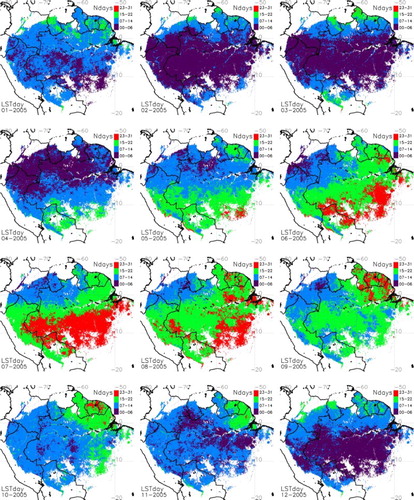
Figure 2. Same as Figure 1, for nighttime LST.

Therefore, the use of daytime LST is preferred so as to increase the spatial coverage over the study area. Moreover, the mean LST computed from the average value between daytime and nighttime LSTs is also affected, since it incorporates the missing data in the nighttime acquisitions.

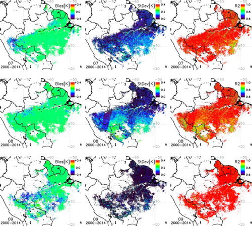
Note that monthly means in the MODrep product are only computed when at least 15 days of valid data are available (green and red colors in Figures 1 and 2), so the spatial coverage of this product is dramatically reduced for the months with a low number of valid days. This reduction is illustrated in Figure 3, which shows that the MODrep product is most useful for analysis of the JAS season (or particular months between May and September). Figure 3 also shows that both products provide similar spatial patterns of thermal anomalies. This fact is corroborated in Figure 4, which shows the differences between the two products (MOD11C3 minus MODrep) for the JAS season months. Bias for the three months is close to zero or slightly negative (thus MOD11C3 providing lower values than MODrep), with standard deviations typically below 0.1 K. The coefficient of determination is above 90%.

Figure 3. Comparison between seasonal standardized anomalies obtained from MOD11C3 and MODrep products in the year 2010.

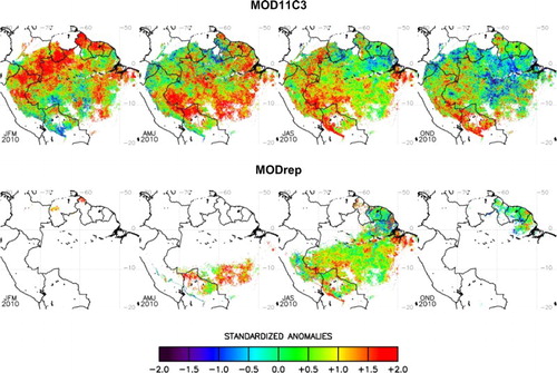
Figure 4. Differences between MOD11C3 and MODrep products for the months July, August, and September, and the period 2000–2014. Maps display bias, standard deviation (StDev), and coefficient of determination (R²).

3.1.2. Effect of fires and smoke plumes

The occurrence of fires during the dry season and severe drought events is a characteristic particular to the Amazon Basin (e.g. Brando et al. 2014). Therefore, these high temperature events can lead to alterations in the computation of the monthly mean temperature, as does aerosol contamination due to smoke plumes. However, smoke plumes are composed of fine particles as compared to the TIR wavelengths, so smoke plumes are penetrated by TIR radiation and the scattering is much less critical than it is in the case of VNIR radiation (Sabins 2000).

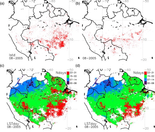
Since pixels with anomalous high temperatures (LST values > LSTmean + 3σ) are removed in the MODrep product, hot spots are expected to be removed from the monthly mean calculation. Figure 5 shows an example of hot spots detected by the MOD14 product, and the outliers removed from the monthly mean temperature calculation in the MODrep product. It can be observed that outliers include almost all the hot spots included in the MOD14, although the number of outliers is higher than the number of MOD14 hot spots because it also includes other anomalous values. Figure 5 also shows the number of valid days when the ±3σ filter is applied, and the number of valid days when the hot spots included in the MOD14 product are also filtered. Only small changes are observed, since most of the hot spots are already included in the filtered outliers. The difference between the surface temperatures obtained in these two cases (results not shown) is typically below 0.2 K.

Figure 5. (a) Pixels removed from the monthly mean computation in the MODrep product after application of the 3s filter. (b) Hot spots (fires with a confidence level > 75%) included in the MOD14 product. (c) Number of valid days to compute the monthly mean in the MODrep product, and (d) number of valid days after removal of MOD14 hot spots. Results are presented for the monthly daytime LST in August 2005.

The analysis of the MODIS aerosol product (MOD08) evidenced a widespread anomalous high aerosol content (AOD > 0.6) during the dry season, mainly in August and September, and especially in 2005, 2007, and 2010 (results not shown). Therefore, the application of an aerosol filter dramatically reduces the available number of valid pixels and the final monthly product is practically useless for the analysis of thermal anomalies. This result may be unrealistic since spatial patterns of standardized anomalies (without the aerosol filter) seem to be realistic (see Section 3.2), which could be explained by the high penetration of the thermal signal through the smoke plume. In fact, LST algorithms based on the split-window technique (the MOD11 product is partly based on this algorithm) are less sensitive to the optical properties of the atmosphere, and radiative transfer simulations in the TIR region focus mainly on atmospheric absorption due to water vapor, thus neglecting scattering processes due to aerosol content (e.g. Wan and Dozier 1996; Wan and Li 1997).

3.2. Intercomparison between MOD11C3 and ERA-Interim

3.2.1. Surface temperature anomalies

The spatial pattern of standardized anomalies obtained from MOD11C3 and ERA-Interim products for the JAS season during the period 2000–2014 is presented in Figures 6 and 7, respectively. For a better intercomparison between the two products, MOD11C3 spatial resolution (0.05°) was degraded to the ERA-Interim spatial resolution (0.75°). Both products typically provide a similar spatial pattern in terms of standardized anomalies. A predominant cooling can be observed in the years prior to the first severe drought of 2005, except for year 2002, which shows almost a neutral pattern. On the contrary, a nearly sustained warming is observed from years 2005 to 2014, with the year 2013 being an exception.

Figure 6. Standardized thermal anomalies obtained from MODIS MOD11C3 product for the JAS season and the period 2000–2014. MODIS images were resampled to 0.75°.

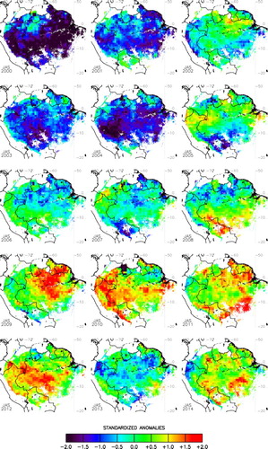
Figure 7. Standardized thermal anomalies obtained from the ERA-Interim skin temperature product (0.75°) for the JAS season and the period 2000–2014.

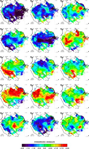
However, some differences between the two products over particular regions and/or periods can also be observed. In the case of 2005, the warmed regions are more enhanced in the ERA-Interim product, with standardized anomalies above +1.5, while warmed regions in the MOD11C3 show values between +1 and +1.5. Despite the different values, the locations of the warmed regions are similar. Significant differences between the two products are observed over western Amazonia in the years 2006, 2009, and 2012. In the years 2006 and 2009, MOD11C3 shows a neutral pattern, whereas ERA-Interim clearly shows a warming. In the case of 2012, MOD11C3 shows warming and ERA-Interim shows cooling.

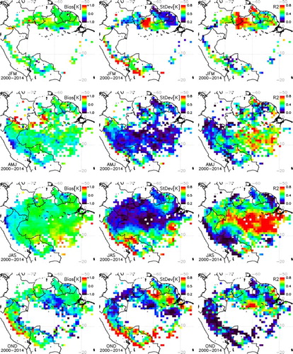
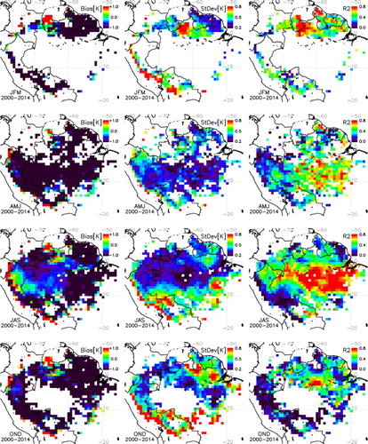
Although maps of standardized anomalies are a useful tool for identifying anomalous warming or cooling via visual inspection, it is also worth analyzing the differences in terms of absolute anomalies. Figure 8 shows some basic statistics (bias, standard deviation, and coefficient of determination) for the difference between MOD11C3 and ERA-Interim products for different seasons and the period 2000–2014 (or 2001–2014 in the case of JFM season). In order to compute the difference between MOD11 (0.05°) and ERA-Interim (0.75°) LST anomalies, MODIS values were averaged using a kernel of 15×15 pixels. Because of missing data in the MODIS products, the difference was also computed when at least 75% of the pixels in the kernel were available. Results show a bias close to zero, with standard deviations around 0.2 K in most regions. However, enormous differences (∼0.8 K) can also be observed over particular regions, especially in the OND season. Values of R² between 50% and 80% are observed in most cases, especially over eastern Amazonia and the JAS season, with the OND season providing the lowest values of R². The highest standard deviation values and the lowest R² values observed in the westernmost pixels in Peru may be attributed to a ‘border effect’ caused by the coarse spatial resolution of the ERA-Interim data, which implies that these pixels located on the border between the Peruvian ‘Cordillera Blanca’ and the Peruvian Amazon are not really pure EBF pixels.

Figure 8. Differences in surface temperature anomalies between MOD11C3 and ERA-Interim products for different seasons and the period 2000–2014. Maps display bias, standard deviation (StDev), and coefficient of determination (R²).

The differences between the MOD11C3 and ERA-Interim products were also assessed by analyzing the time series of the absolute anomalies over particular pixels. As an illustrative example, Figure 9 includes the time series of LST absolute anomalies for the four seasons and for two arbitrarily selected pixels, one pixel with a poor correlation between MOD11C3 and ERA-Interim (R² between 0 and 0.3), and one pixel with a high correlation between the two products (R² between 0.6 and 0.8).

Figure 9. Time series of seasonal LST absolute anomalies since 2000 extracted from MOD11C3 and ERA-Interim products for two particular pixels: (i) one pixel located in southwestern Amazonia (left column; central coordinates of the pixel −10.25N, −70.25E), with a poor correlation between the two products, and (ii) one pixel located in eastern Amazonia (right column; central coordinates of the pixel −4.25N, −53E), with a high correlation between the two products.

The pixel with a low correlation (left column in Figure 9) is located in the southwestern Amazon, and it evidences significant differences between the two products over particular years. For example, ERA-Interim provides an anomaly close to zero in 2004 during the JFM season, whereas the MODIS product provides an anomaly higher than +1 K. A similar result is observed in the JAS and OND seasons for year 2006. The differences observed between the two products in the years 2005 and 2010 for the JAS season are particularly remarkable. Results are consistent for the pixel with a good correlation (right column, Figure 9), located in eastern Amazon, although a difference between the two products of around 1 K is observed in the year 2010 for the JAS season.

3.2.2. Absolute surface temperatures

Despite our focus on the analysis of thermal anomalies, a brief analysis of the differences in absolute surface temperatures is valuable for further understanding the differences observed in the anomalies of the two datasets presented in the previous section.

Figure 10 illustrates the difference between surface temperatures included in the MOD11C3 and ERA-Interim products for different seasons. When compared to Figure 8 (where temperature anomalies are compared), similar standard deviations and correlations (R²) can be observed. However, the bias (MOD11C3 minus ERA-Interim) is significantly different, with negative values (up to −1 K) in most cases. This bias is partly reduced in the JAS season, with a higher occurrence of cloud-free days and higher values of temperatures than in other seasons. The comparison between the climatological means (2001–2013) obtained with the two datasets also provides a similar bias (results not shown). Since temperature anomalies are obtained after subtraction of the climatological mean (Equation (1)), the bias is partly offset. This may explain the lower bias observed in the comparison between temperature anomalies obtained with the two datasets (Figure 8).

Figure 10. Differences in (absolute) surface temperature between MOD11C3 and ERA-Interim products for different seasons and the period 2000–2014. Maps display bias, standard deviation (StDev), and coefficient of determination (R²).

3.3. Trends in surface temperature anomalies

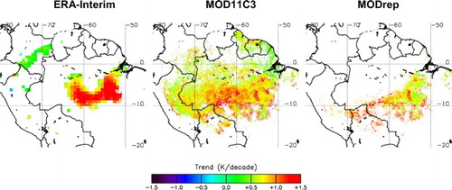
We finish off the analysis by intercomparing the trends in surface temperature anomalies computed from the different products. Figure 11 shows the trends in the JAS season for the period 2000–2014 computed from the ERA-Interim, MOD11C3 and MODrep surface temperature anomalies products. The most striking spatial feature is the significant warming observed in the three products over southeastern Amazonia, with warming rates higher than 1.5°C/decade in most cases. When the ERA-Interim product is compared to MOD11C3, it is observed that ERA-Interim does not provide a significant warming rate over eastern Amazonia. MODrep results are consistent with results obtained from the MOD11C3 product, although the spatial coverage is greatly reduced as mentioned in Section 3.2.

Figure 11. Trends in surface temperature anomalies for the JAS season during the period 2000–2014 using the different LST products. Only pixels with p < .05 are displayed.

Figure 12 includes the scatter plots of temperature trends obtained using the different products. When MOD11C3 is compared to ERA-Interim, a bias of 0.3 ± 0.4°C/decade is obtained when all the data points are considered. The bias is reduced to −0.1 ± 0.5°C/decade when only trend values with p < .05 are considered. Results are improved when MOD11C3 is compared to MODrep, with bias values of 0.1 ± 0.3°C/decade for all the data points and 0.1 ± 0.2°C/decade for data points with p < .05.

Figure 12. Scatter plots of trends in surface temperature anomalies (2000–2014) obtained from the MOD11C3 product versus (a) the ERA-Interim product and (b) the MODrep product. Bias and standard deviation are provided when all the data points are considered, as well as when only trend values significant at p < .05 are considered. Dashed lines represent the linear fit.

Finally, Figure 13 shows the surface temperature anomalies trends over different longitudinal transects. Trends provided by ERA-Interim are typically lower than those provided by MOD11C3, except for the eastern part of the transect at –8N. In general, longitudinal variations of the trend are smooth, although some asymmetries are observed for transects located at the lower latitudes (approximately below 4S).

Figure 13. Intercomparison of trends in surface temperature anomalies (2000–2014) obtained from ERA-Interim and MOD11C3 products over different longitudinal transects. Values marked with an asterisk indicate statistical significance at p < .05.

4. Summary and conclusions

Analysis of thermal anomalies over the Amazon forests is a key issue for understanding the forest response to droughts and potential impact on carbon absorption, especially after the occurrence of two major droughts in a short time span. However, it has received less attention than the analysis of anomalies of vegetation indices, with several publications providing different and contradictory results. In order to better understand the results extracted from surface temperature products over the Amazon forest, we intercompared thermal anomalies obtained from two independent datasets, such as remote sensing (MODIS) and reanalysis (ERA-Interim) products. The intercomparison of the spatial pattern of standardized anomalies showed that both MODIS and ERA-Interim products are typically consistent, although some differences were observed over particular regions and the warmed regions are sometimes enhanced differently. Differences in absolute anomalies can be critical when intercompared over particular pixels and months/seasons, with differences around 1 K, although the bias was typically maintained around zero with a standard deviation of 0.2 K. Differences in surface temperature anomalies trends were also observed between the two products, up to 0.5°C/decade. However, the spatial pattern of the trends in both cases showed a significant warming during the JAS season over southeastern Amazonia, as presented in Jiménez-Muñoz et al. (2013). This significantly warmed area mainly affects the phenoregions 3, 4, and 24 described in Silva et al. (2013), which includes a forest of low lands and forest transition between dense, open forest, and savanna.

Using the reprocessing of the daily MODIS LST product as a basis, we also presented a new monthly LST computation, where outliers are removed from the mean calculation (MODrep). Moreover, the monthly values are only computed if at least 50% of the values within one month (∼15 days) are available. Because of the cloud contamination during the rainy season (approximately from January to April and from October to December), in the MODrep product the spatial coverage is dramatically reduced over nearly the entire Amazon basin. During the dry season (approximately from May to September), only southern Amazonia provided valid pixels. Some regions located in northern Amazonia also provided valid pixels for the periods January–April and October–December due to differences in the occurrence of the peak in the dry season (Silva et al. 2013). In a preliminary analysis, it was also observed that the MODrep product removes pixels affected by active fires due to the application of the outliers removal filter, but this requires further analysis. The effect of the smoke plumes (anomalous high values of aerosol content) on surface temperature anomalies is uncertain, since thermal radiation can penetrate the smoke plume and the scattering is weaker than it is in the case of VNIR. This issue also requires further research. Results presented in this paper show that remote sensing and climatic products are useful tools for the analysis of the spatial pattern of standardized anomalies or temperature trends, but absolute values should be taken with caution because of the differences observed between the products. Datasets used in this study can be visualized and downloaded at the Thermal Amazoni@ geoportal available at the following link http://ipl.uv.es/thamazon/web (Jiménez-Muñoz et al. 2015).

Supplemental data

Supplemental data for this article can be accessed at http://dx.doi.org/10.1080/17538947.2015.1056559.

Acknowledgements

The authors would like to thank the editor and anonymous reviewers for their constructive comments and suggestions to improve the paper.

Disclosure statement

No potential conflict of interest was reported by the authors.

Funding

This work was partly funded by the University of Valencia [UV-INV-PRECOMP13-115366], Ministerio de Ciencia e Innovación [CEOS-Spain, AYA2011-29334-C02-01], CONICYT [Fondecyt Iniciacion – 1130359] and the University of Chile [Ayuda U Viajes, VID-Uchile 2014–2015].

References

- Balsamo, G., C. Albergel, A. Beljaars, S. Boussetta, E. Brun, H. Cloke, D. Dee, et al. 2015. “ERA-Interim/Land: A Global Land Surface Reanalysis Data Set.” Hydrology and Earth System Sciences 19: 389–407. doi: 10.5194/hess-19-389-2015
- Brando, P. M., J. K. Balch, D. C. Nepstad, D. C. Morton, F. E. Putz, M. T. Coe, D. Silverio, et al. 2014. “Abrupt Increases in Amazonian Tree Mortality due to Drought-fire Interactions.” Proceedings of the National Academy of Sciences 111 (17): 6347–6352. doi: 10.1073/pnas.1305499111
- Clark, D. A., S. C. Piper, C. D. Keeling, and D. B. Clark. 2003. “Tropical Rain Forest Tree Growth and Atmospheric Carbon Dynamics Linked to Interannual Temperature Variation During 1984–2000.” Proceedings of the National Academy of Sciences 100 (10): 5852–5857. doi: 10.1073/pnas.0935903100
- Czajkowski, K. P., Goward, S. N., Mulhern, T., Goetz, S. J., Walz, A., Shirey, D., Stadler, S., Prince, S. D., and R. O. Dubayah. 2000. “Estimating Environmental Variables Using Thermal Remote Sensing.” In Thermal Remote Sensing in Land Surface Processes, edited by D. A. Quattrochi and J. C. Luvall, 11–32. Boca Raton, FL: CRC Press.
- Dee, D. P., S. M. Uppala, A. J. Simmons, P. Berrisford, P. Poli, S. Kobayashi, U. Andrae, et al. 2011. “The ERA Interim Reanalysis: Configuration and Performance of the Data Assimilation System.” Quarterly Journal of the Royal Meteorological Society 137: 553–597. doi: 10.1002/qj.828
- Dessler, A. E. 2010. “A Determination of the Cloud Feedback from Climate Variations Over the Past Decade.” Science 330 (6010): 1523–1527. doi: 10.1126/science.1192546
- Doughty, C. E., and M. L. Goulden. 2008. “Are Tropical Forests Near a High Temperature Threshold?” Journal of Geophysical Research 113. G00B07. doi:10.1029/2007JG000632.
- Fréville, H., E. Brun, G. Picard, N. Tatarinova, L. Arnaud, C. Lanconelli, C. Reijmer, and M. van den Broeke. 2014. “Using MODIS Land Surface Temperatures and the Crocus Snow Model to Understand the Warm Bias of ERA-interim Reanalyses at the Surface in Antarctica.” The Cryosphere 8: 1361–1373. doi:10.5194/tc-8-1361-2014.
- Galbraith, D., P. E. Levy, S. Sitch, C. Huntingford, P. Cox, M. Williams, and P. Meir. 2010. “Multiple Mechanisms of Amazonian Forest Biomass Losses in Three Dynamic Global Vegetation Models Under Climate Change.” New Phytologist 187: 647–665. doi:10.1111/j.1469-8137.2010.03350.x.
- Gatti, L. V., M. Gloor, J. B. Miller, C. E. Doughty, Y. Malhi, L. G. Domingues, L. S. Basso, et al. 2014. “Drought Sensitivity of Amazonian Carbon Balance Revealed by Atmospheric Measurements.” Nature 506: 76–80. doi: 10.1038/nature12957
- Giglio, L., J. Descloitres, C. O. Justice, and Y. Kaufman. 2003. “An Enhanced Contextual Fire Detection Algorithm for MODIS.” Remote Sensing of Environment 87: 273–282. doi: 10.1016/S0034-4257(03)00184-6
- Hilker, T., A. I. Lyapustin, C. J. Tucker, F. G. Hall, R. B. Myneni, Y. Wang, J. Bi, Y. Mendes de Moura, and P. J. Sellers. 2014. “Vegetation Dynamics and Rainfall Sensitivity of the Amazon.” Proceeding of the National Academy of Sciences 111 (45): 16041–16046. doi: 10.1073/pnas.1404870111
- Hubanks, P. A., M. D. King, S. Platnick, and R. Pincus. 2008. “MODIS Atmosphere L3 Gridded Product.” Algorithm Theoretical Basis Document. http://modis-atmos.gsfc.nasa.gov/_docs/L3_ATBD_2008_12_04.pdf.
- Jackson, R. D., S. B. Idso, R. J. Reginato, and P. J. Pinter. 1981. “Canopy Temperature as a Crop Stress Indicator.” Water Resources Research 4: 1133–1138. doi: 10.1029/WR017i004p01133
- Jiménez-Muñoz, J. C., C. Mattar, J. A. Sobrino, and Y. Malhi. 2015. “A Database for the Monitoring of Thermal Anomalies Over the Amazon Forest and Adjacent Intertropical Oceans.” Scientific Data. doi:10.1038/sdata.2015.24.
- Jiménez-Muñoz, J. C., J. A. Sobrino, and C. Mattar. 2013. “Has the Northern Hemisphere Been Warming or Cooling During the Boreal Winter of the Last Few Decades?” Global and Planetary Change 106: 31–38. doi: 10.1016/j.gloplacha.2013.02.010
- Jiménez-Muñoz, J. C., J. A. Sobrino, C. Mattar, and Y. Malhi. 2013. “Spatial and Temporal Patterns of the Recent Warming of the Amazon Forest.” Journal of Geophysical Research 118: 5204–5215.
- Kendall, M. G. 1975. Rank Correlation Methods. 4th ed. London: Charles Griffin.
- Lewis, S. L., P. M. Brando, O. L. Phillips, G. M. F. van der Heijden, and D. Nepstad. 2011. “The 2010 Amazon Drought.” Science 331: 554. doi: 10.1126/science.1200807
- Malhi, Y., J. Timmons Roberts, R. A. Betts, T. J. Killeen, W. Li, and C. A. Nobre. 2008. “Climate Change, Deforestation, and the Fate of Amazon.” Science 319: 169–172. doi: 10.1126/science.1146961
- Malhi, Y., D. Wood, T. R. Baker, J. Wright, O. L. Phillips, T. Cochrane, P. Meir, et al. 2006. “The Regional Variation of Aboveground Live Biomass in Old-growth Amazonian Forests.” Global Change Biology 12: 1107–1138. doi: 10.1111/j.1365-2486.2006.01120.x
- Marengo, J. A., C. A. Nobre, J. Tomasella, M. D. Oyama, G. S. de Oliveira, R. de Oliveira, H. Camargo, L. M. Alves, and I. Foster Brown. 2008. “The Drought of Amazonia in 2005.” Journal of Climate 21 (3): 495–516. doi: 10.1175/2007JCLI1600.1
- Masters, T. 2012. “On the Determination of the Global Cloud Feedback from Satellite Measurements.” Earth System Dynamics 3: 97–107. doi: 10.5194/esd-3-97-2012
- Morton, D. C., J. Nagol, C. C. Carabajal, J. Rosette, M. Palace, B. D. Cook, E. F. Vermote, D. J. Harding, and P. R. J. North. 2014. “Amazon Forests Maintain Consistent Canopy Structure and Greenness During the Dry Season.” Nature 506: 221–224. doi: 10.1038/nature13006
- Phillips, O. L., L. E. O. C. Aragao, S. L. Lewis, J. B. Fisher, J. Lloyd, G. López-González, Y. Malhi, et al. 2009. “Drought Sensitivity of the Amazon Rainforest.” Science 323: 1344–1347. doi: 10.1126/science.1164033
- Saatchi, S., S. Asefi-Najafabady, Y. Malhi, L. E. O. C. Aragao, L. O. Anderson, R. B. Myneni, and R. Nemani. 2013. “Persistent Effects of a Severe Drought on Amazonian Forest Canopy.” Proceedings of the National Academy of Sciences 110 (2): 565–570. doi: 10.1073/pnas.1204651110
- Sabins, F. F. 2000. Remote Sensing. Principles and Interpretation. 3rd ed. USA: W. H. Freeman and Company.
- Saleska, S. R., K. Didan, A. R. Huete, and H. R. da Rocha. 2007. “Amazon Forests Green-up During 2005 Drought.” Science 318: 612. doi: 10.1126/science.1146663
- Samanta, A., S. Ganguly, H. Hashimoto, S. Devadiga, E. Vermote, Y. Knyazikhin, R. R. Nemani, and R. B. Myneni. 2010. “Amazon Forest did not Green-up During the 2005 Drought.” Geophysical Research Letters 37: L05401. doi:10.1029/2009GL042154.
- Schroeder, W., E. Prins, L. Giglio, I. Csiszar, C. Schimdt, J. Morisette, D. Morton. 2008. “Validation of GOES and MODIS Active Fire Detection Products using ASTER and ETM+ Data.” Remote Sensing of Environment 112: 2711–2726. doi: 10.1016/j.rse.2008.01.005
- Screen, J. A., and I. Simmonds. 2010. “The Central Role of Diminishing sea Ice in Recent Arctic Temperature Amplification.” Nature 464: 1334–1337. doi: 10.1038/nature09051
- Sen, P. K. 1968. “Estimates of the Regression Coefficient Based on Kendall's Tau.” Journal of the American Statistical Association 63: 1379–1389. doi: 10.1080/01621459.1968.10480934
- Silva, F. B., Y. E. Shimabukuro, L. E. O. C. Aragao, L. O. Anderson, G. Pereira, F. Cardozo, and E. Arai. 2013. “Large-scale Heterogeneity of Amazonian Phenology Revealed from 26-year Long AVHRR/NDVI Time-series.” Environmental Research Letters 8: 024011. doi:10.1088/1748-9326/8/2/024011.
- Simmons, A. J., K. M. Willett, P. D. Jones, P. W. Thorne, and D. P. Dee. 2010. “Low-frequency Variations in Surface Atmospheric Humidity, Temperature and Precipitation: Inferences from Reanalyses and Monthly Gridded Observational Datasets.” Journal of Geophysical Research 115: 1–21. doi:10.1029/2009JD012442.
- Strahler, A., D. Muchoney, J. Borak, M. Friedl, S. Gopal, E. Lambin, and A. Moody. 1999. MODIS Land Cover Product, Algorithm Theoretical Basis Document Version 5.0. Boston, MA: Boston University.
- Toomey, M., D. A. Roberts, C. Still, M. L. Goulden, and J. P. McFadden. 2011. “Remotely Sensed Heat Anomalies Linked with Amazonian Forest Biomass Declines.” Geophysical Research Letters 38: L19704. doi:10.1029/2011GL049041.
- Tsuang, B.-J., M.-D. Chou, Y. Zhang, A. Roesch, and K. Yang. 2008. “Evaluations of Land-Ocean Skin Temperatures of the ISCCP Satellite Retrievals and the NCEP and ERA Reanalyses.” Journal of Climate 21 (2): 308–330. doi:10.1175/2007JCLI1502.1.
- Viterbo, P., and A. C. M. Beljaars. 1995. “An Improved Land Surface Temperature Parameterization Scheme in the ECMWF Model and its Validation.” Journal of Climate 8: 2716–2748. doi: 10.1175/1520-0442(1995)008<2716:AILSPS>2.0.CO;2
- Wan, Z. 2007. Collection-5 MODIS Land Surface Temperature Products Users’ Guide, ICESS. Santa Barbara, CA: University of California.
- Wan, Z. 2008. “New Refinements and Validation of the MODIS Land-surface Temperature/Emissivity Products.” Remote Sensing of Environment 112: 59–74. doi: 10.1016/j.rse.2006.06.026
- Wan, Z., and J. Dozier. 1996. “A Generalized Split-window Algorithm for Retrieving Land-surface Temperature from Space.” IEEE Transactions on Geoscience and Remote Sensing 34 (4): 892–905. doi: 10.1109/36.508406
- Wan, Z., and Z.-L. Li. 1997. “A Physics-based Algorithm for Retrieving Land-surface Emissivity and Temperature from EOS/MODIS Data.” IEEE Transactions on Geoscience and Remote Sensing 35 (4): 980–996. doi: 10.1109/36.602541
- Zhou, L., Y. Tian, R. B. Myneni, P. Ciais, S. Saatchi, Y. Y. Liu, S. Piao, et al. 2014. “Widespread Decline of Congo Rainforest Greenness in the Past Decade.” Nature 509: 86–90. doi: 10.1038/nature13265