Comparisons of two global built area land cover datasets in methods to disaggregate human population in eleven countries from the global South

ABSTRACT

Mapping built land cover at unprecedented detail has been facilitated by increasing availability of global high-resolution imagery and image processing methods. These advances in urban feature extraction and built-area detection can refine the mapping of human population densities, especially in lower income countries where rapid urbanization and changing population is accompanied by frequently out-of-date or inaccurate census data. However, in these contexts it is unclear how best to use built-area data to disaggregate areal, count-based census data. Here we tested two methods using remotely sensed, built-area land cover data to disaggregate population data. These included simple, areal weighting and more complex statistical models with other ancillary information. Outcomes were assessed across eleven countries, representing different world regions varying in population densities, types of built infrastructure, and environmental characteristics. We found that for seven of 11 countries a Random Forest-based, machine learning approach outperforms simple, binary dasymetric disaggregation into remotely-sensed built areas. For these more complex models there was little evidence to support using any single built land cover input over the rest, and in most cases using more than one built-area data product resulted in higher predictive capacity. We discuss these results and implications for future population modeling approaches.

KEYWORDS:

• Land cover
• built areas
• remote sensing
• settlement mapping
• population modeling

1. Introduction

Improvements in detecting and estimating changes in built land cover from remotely-sensed data have important scientific applications. One such application is estimating where and in what density humans live on the Earth's surface, a research area that is hugely informed by a variety of remotely sensed data that are not limited to just land cover (e.g. Anderson and Anderson 1973; Lo 1995; Sutton et al. 2001; Linard et al. 2010; Sorichetta et al. 2015; Stevens et al. 2015). But of all these data sources, built-up and settlement locations are the single most highly predictive indicator of human habitation (Stevens et al. 2015; Sorichetta et al. 2015). Improvements in these measurements will highly influence fine-scale estimates of human population density. Better estimates of where people live yield advances in disaster and risk management, development and planning, human health, epidemiology, and other issues regarding land use and the sustainability of many types of human activities. Considering these applications, improvements in both built area mapping and population modeling are especially critical to assess in lower and middle-income countries in the Global South, where urbanization and population growth is accompanied by demand for better data.

Here we present a study of how different built-area representations, derived from a variety of past and recent remote-sensing approaches, affect our ability to predict where and in what density human populations are distributed using two common methods. The objective of the paper is primarily to assess how two different population mapping approaches perform when informed by two global, publicly available built area data sets. It is at this intersection of the modeling approaches with the data used, in low and middle-income countries, that yields insight into the how future population estimation might better be conducted.

1.1. Remote sensing of built-areas

Over the last two decades the availability of remotely sensed data products with varying spatial, temporal, and sensor characteristics has increased and global data products continue to expand (Grekousis, Mountrakis, and Kavouras 2015). These data combined with increased computer processing power and new algorithms for classification has led to a proliferation of global built-area datasets that have been well summarized and compared (Florczyk et al. 2019). An important constraint to producing land cover, and specifically built area data at near global extents is the availability of contemporaneous and contiguous remotely sensed data. Such efforts include optically-derived analyses from multiple Landsat sensors (e.g. Bontemps et al. 2011; Pesaresi et al. 2015), MODIS (e.g. Potere et al. 2009; Schneider, Friedl, and Potere 2010), ENVISAT MERIS (e.g. ESA 2017) among others. Newer and more sophisticated approaches include data collected from active sensors, such as radar, sometimes in combination with optical data (e.g. Corbane et al. 2017; Esch et al. 2013). The products we consider here as representatives are among the newest, and widely used sources of built area data that have been produced and released as near-global extents. The products include the Global Human Settlement Layer Landsat product (GHSL) which is an optically-derived product, relying on multiple Landsat sensors (Pesaresi et al. 2015, 2016). GHSL products, produced by the European Commission Joint Research Centre (JRC), include estimates for built-areas circa 1975, 1990, 2000 and 2014. The second built area data set we test is the Global Urban Footprint developed by the German Aerospace Center (DLR), which uses radar-derived data and is currently available to the public at a 78-meter and 12-meter spatial resolution for the year 2012 (Esch et al. 2013). We also utilize lower resolution datasets that are specific to urban footprints or include built land cover classes and include the MODIS (Moderate Resolution Imaging Spectroradiometer)-derived 500-meter global built area product for 2000 (Schneider, Friedl, and Potere 2009) and the European Space Agency's CCI Land Cover series of 300-meter ENVISAT MERIS-derived land cover datasets (circa 2000, 2005, and 2010) (ESA 2017). It is important to note that we are considering here only data that are publically available and free to download, under a permissive license, and produced using openly documented methods.

1.2. Gridded estimates of human population density

The simplest approaches that produce gridded estimates of population have relied on either isometric areal weighting or dasymetric (weighted by an ancillary data source) techniques to redistribute census counts to grid cells within administrative areas (e.g. Small and Nicholls 2003; Balk and Yetman 2004; CIESIN 2017). More complex methods have relied on combinations of ancillary data layers (e.g. land cover, nighttime lights) and their statistically measured relationships with population density to either directly predict population within grid cells or weight the disaggregation of census counts (e.g. Dobson et al. 2000; Bhaduri et al. 2007; Linard et al. 2010; Roy and Blaschke 2014; Stevens et al. 2015; Gaughan et al. 2016). Based on the approach used gridded products may also represent different types of population, such as residential (e.g. Stevens et al. 2015) or ambient populations (Dobson et al. 2000).

For those approaches using ancillary data, we might describe those along a spatial modeling spectrum of dasymetric-driven methods to more complex, multi-variable statistical techniques (Stevens et al. 2015; Mennis 2003; Mennis 2009) Dasymetric techniques can take different forms but commonly incorporate a binary masking in which grid cells are either populated or unpopulated based on an underlying ancillary data source (Mennis and Hultgren 2006). In more complex methods counts are redistributed by using weights within populated cells using other data or models. Regardless of a disaggregation method's complexity, the accuracy of the gridded estimate is greatly affected by the spatial resolution and accuracy of the census data driving them (Deville et al. 2014). The census data will affect the predictive accuracy of the statistical models which are used to provide pixel-level estimates (Gaughan et al. 2014), or the spatial fidelity and weight per unit area for dasymetric redistributions. Well known and commonly used global and regional gridded population estimates that fall along the spectrum of simple areal weighting to more statistically complex techniques include the Gridded Population of the World (GPW), now on its 4th version (CIESIN 2017), datasets from the WorldPop Project (Stevens et al. 2015), ESRI's World Population Estimated (WPE) data set (Frye, Nordstrand, and Environmental Systems Research Institute 2017), GHS-POP (European Commission Joint Research Centre and Columbia University Center for International Earth Science Information Network 2015) and the LandScan products (Dobson et al. 2000), among others. These products have gridded regional and global coverage with spatial resolutions that range from ∼100 m to 1 km at the equator and with multiple estimations through time at either a country- or global-level extent. These data and more information about their production and usage are now described by the POPGRID Data Collaborative, a clearinghouse for gridded population data producer information and training (https://popgrid.org).

1.3. Built-areas and population modeling

Since the 1990s, gridded representations of human populations have provided valuable, spatially-explicit information about population distribution. The advances in high-resolution satellite-based products provide a valuable source of data informing population maps, data which is relied on in the bottom-up and hybrid types of population modeling. For example, these newer high-resolution satellite products are used in the ‘lightly-modeled’ binary dasymetric (BD) mapping approach by concentrating total population counts of an administrative area into the grid cells within that area classified as settlement. This approach was recently applied in collaboration between the Center for International Earth Science Information Network (CIESIN) and Facebook's Connectivity Lab and their High Resolution Settlement Layer (HRSL) (Facebook Connectivity Lab and Columbia University Center for International Earth Science Information Network 2017) and is similar to others using GUF to disaggregate population into built areas (Merkens and Vafeidis 2018). Built area data produced at relatively fine resolution might also be aggregated to estimate built area density, and used as a non-binary dasymetric weighting layer, such as the technique used by CIESIN and the Joint Research Center to produce GHS POP (Freire et al. 2016). Other ways of integrating built-area data include incorporating the settlement layers as one or more covariates using a more highly modeled approach to generate final population values (Stevens et al. 2015; Dobson et al. 2000; Azar et al. 2013; e.g. Azar et al. 2010). The extreme treatments of the data, binary dasymetric and statistically modeled, have improved on our ability to concentrate census counts in more spatially explicit and accurate ways but derive value and errors from built area data in very different ways. But it remains unclear which type of approach is more accurate to disaggregating census counts and generating gridded population maps using common, freely available global data products.

Previous work has stressed the importance of remotely-sensed estimates and proxies for the built environment (e.g. nighttime lights, settlement, impervious surfaces) as key components towards accurate production of human population distribution datasets (Nieves 2016; Nieves et al. 2017). Here we extend such findings by producing systematic tests of the contributions to population mapping that a range of remotely-sensed, built-area and settlement data make in simple binary dasymetric (BD) areal weighting (Freire et al. 2016; Facebook Connectivity Lab and Columbia University Center for International Earth Science Information Network 2017) and multivariate Random Forest (RF) machine learning weighted dasymetric estimates (Stevens et al. 2015). We compare how data derived from optical and radar-based remote sensing products might improve these population estimates from each approach and take into consideration the accuracy and comparability of these remotely-sensed built-area datasets in low and middle-income countries.

2. Methods and data descriptions

2.1. Study areas

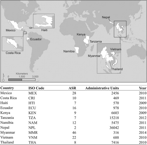
Model comparisons were done for eleven countries, identified in Figure 1 with their associated census data. The selected countries represent different regions (e.g. South and Central America, Africa, and Asia) but most importantly provide variation in population densities, built infrastructure types, and physical environmental characteristics, all of which are important with respect to associations with population density and model performance. We also focused on these because each country had circa-2010 census data available at relatively fine spatial resolutions with enough coarsened data to estimate models, while leaving fine data for assessing disaggregation efficiency within each country. The focus of the modeling in this study is on the disaggregation of census counts and therefore focuses on residential population data. A comparison between each country's census data and its spatial ‘grain’ is represented by its average spatial resolution (ASR) and is calculated as the square root of the country area (sq. km) divided by the total number of units and where smaller numbers indicate more finely-resolved inputs (adapted from Balk and Yetman 2004; Tobler et al. 1997).

Figure 1. Study area countries representing various continental sub-regions around the world. Model countries, defined by ISO code, include Tanzania (TZA), Namibia (NAM), Kenya (KEN), Mexico (MEX), Haiti (HTI), Ecuador (ECU), Costa Rica (CRI), Myanmar (MMR), Thailand (THA), Vietnam (VNM), and Nepal (NPL). Census data sources are provided per country in Supplemental Information S4.

2.2. Data descriptions

The highest spatial resolution, most contemporary census-based population data linked to administrative boundaries available were acquired for each country (Figure 1). In addition, a ‘coarsened’ version of each country's data was produced by merging one-third of the administrative units, selected randomly, with their neighboring administrative unit with the longest shared border (and which had already not been merged with another unit) and their population counts summed. These merged administrative units were then used for assessing the disaggregation process (explained in more detail in section 2.4) since their original population counts at the finest resolution available can be compared with disaggregated counts from the coarsened data.

For each country, a standard set of predictive covariate layers were acquired including areas 10 km outside the country border in order to avoid edge effects (Fotheringham and Rogerson 1993) linked with the fact that while countries are artificially bounded spatial processes are not (Barber 1988; Fotheringham and Rogerson 1993) (Table 1). These covariate layers included: VIIRS nighttime lights (Elvidge et al. 2013), SRTM 3 arcsecond void-filled DEM elevation and DEM derived slope (Farr 2007), precipitation and temperature, sourced from the WorldClim project (Hijmans et al. 2005) and protected areas from the World Database on Protected Areas (WPDA) (IUCN and UNEP 2012). Additionally, distance to rivers, roads, and to the nearest edge of waterbodies was calculated from Open Street Map (OSM) data (OSM 2017) using a ‘distance-to-feature’ criteria. In the case of linear features, it was to the feature or nearest part of the feature (in the case of a road) that positive values were calculated. However, for polygonal features such as waterbodies and land cover types, distance-to-outer edge was calculated to produce positive distance values for areas outside the feature and negative distance values for areas inside them (Gaughan et al. 2016). This approach increases information provided by simple built/non-built data, extending it to provide information at the pixel level relating to areal extent and the configuration of built-area environments such as urban core vs. periphery. Land cover classes of the circa 2010 300 m ESA CCI land cover dataset which were reclassified as in Stevens et al. (2015), and also converted to distance-to-outer-edge (negative cell values are distances within the outer edge of contiguous land cover areas, and positive cell distances fall outside the land cover boundary).

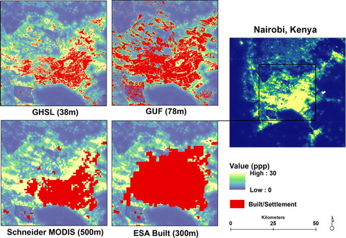
We then compared four different sources of built land cover data (Figure 2) and their influence on the modeling of population distribution. These different sources of built land cover are created using different criteria, whether it be by spectral similarity to impervious surfaces, structural similarity to ‘built-up’ training data, or some combination of these (Esch et al. 2013; Pesaresi et al. 2016; Schneider, Friedl, and Potere 2009; Bontemps et al. 2011). However, the discussion of what constitutes ‘built’ from a remotely-sensed perspective, and how that translates to ‘urban’ or ‘settlement’ on the ground is often even more wide ranging. Despite discussions on definitions, all of these data products are correlated with population distribution. We define built land covers to include human constructed impervious surfaces or settlement areas and included datasets available at the time of analysis that were global, continuous representations of built land cover By doing so, we ensured that the same underlying methods for generating each built dataset was consistent across the study region countries, however, not between data sets.

Figure 2. Comparisons of four different built-area land covers derived from optical (GHSL, Schneider MODIS, ESA) and radar (GUF) sensors are visualized in red. These data at their native resolutions show low levels of agreement. For comparison they are layered on top of population counts (people per pixel (ppp)) estimated using the Random Forest modeling approach using GUF and GHSL built-area estimates as ancillary data.

The first was the built land cover class provided by the circa 2010, 300 m MERIS-derived ESA CCI land cover dataset (ESA 2017). The second was the circa 2000 500 m MODIS urban extents data derived by Schneider, et al. (Schneider, Friedl, and Potere 2010). Both of these were downsampled to 8.33×10^–4 degrees (∼100 m resolution at the equator) using nearest neighbor resampling. The third was the ∼75 m at the equator, Global Urban Footprint (GUF), SAR-derived dataset which was the only available source of GUF data at the time of analysis but which has been superceded by publicly distributed data at 0.4 arc seconds. The final built-area dataset tested was the 38 m Global Human Settlement Layer for 2014. Both of the finer resolution built area data were resampled using a maximum aggregation on a binary, built/non-built realization. All built data were then projected into a country-appropriate UTM projection and processed to calculate the distance-to-built-area-edge prior to modeling. All preprocessing was performed in R 3.2.2 using the ‘raster’ (Hijmans and Van Etten 2012), ‘randomForest’ (Liaw and Wiener 2002), and ‘rgdal’ (Bivand, Keitt, and Rowlingson 2017) packages. Data pre-processing and analyses were conducted in ArcGIS 10.3 and Python 2.7 (see Stevens et al. 2015 for open source code and documentation).

2.3. Gridded population models

2.3.1. BD binary (masked) dasymetric approach

One approach to generate a gridded population map is to conduct dasymetric redistribution where aggregated census datasets are disaggregated to a finer spatial resolution, gridded surface of population counts (Mennis 2003). We produced gridded population estimates using a binary, dasymetric redistribution by masking out any pixel not defined as ‘built’ land cover identified by the underlying ancillary dataset and redistributed census counts to only those grid cells. We describe this as a BD binary dasymetric (BD) weighting. ‘Binary’ refers to the weights assigned to individual pixels which is one if the pixel is classified as built and zero if it is not (Eicher and Brewer 2001). These ones and zeroes are used within each administrative unit to calculate the total number of pixels classified as built-area and then divide the unit's population evenly among all built pixels. The BD redistribution was performed using Python 2.7 and Geospatial Abstraction Library (GDAL) command line tools (GDAL Development Team 2016).

This method is used to produce the High Resolution Settlement Layer (Facebook Connectivity Lab and Columbia University Center for International Earth Science Information Network 2017) and is similar to the approach used in the Global Human Settlement Population Grid data (Freire et al. 2016). We note, that in cases where population counts were nonzero for the administrative unit, but the settlement/urban dataset had no pixels of built land cover then the population was dropped and all pixels within the admin unit were given a value of zero. At the time of our analyses this algorithm was identical to the one employed in beta versions of these data and represents the extreme of simply using built area land cover as a proxy for human populated areas. For public release, however, the algorithms were modified to spread evenly the nonzero population counts across units where built-areas were not detected, thereby conserving the total population counts for each country. When comparing these two alternatives using the metrics presented here and at the pixel level, there were little to no changes in our study countries between zeroing and the uniform areal distribution during the BD approach. This is likely since large deviations in predicted vs. observed population densities tend to dominate the metrics used, and areas with high densities are associated with highly built-up areas where misclassification may be significant but where there will be pixels classified as built by the high-resolution raster data. So in practice, the very small percentage of units that have no built area pixels do not impact the BD disaggregation and the comparison metrics appreciably, relative to the inherent noise incurred by the census and covariate data.

2.3.2. Random Forest (RF) approach

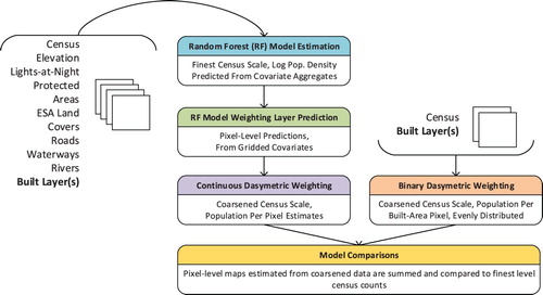
The Random Forest-based hybrid approach is based on a machine-learning model parameterized using census data for mapping populations at fine spatial resolutions (i.e. at three arc seconds and 100 m). As a multi-covariate, statistical approach, it can accommodate a variety of covariates in a nonparametric and robust way, with very few parameters to set. In brief, the method relies on estimating a Random Forest-based model using covariates that are gridded to 100 m pixel sizes. To facilitate between-country comparisons of RF modeling a standardized set of covariates were used for each country. These covariates are derived from those vector- and raster-based data described in Table 1 and illustrated in Figure 3. Each covariate layer, regardless of its spatial representation was converted to a grid/raster, and represented as either a continuous variable (e.g. elevation, light intensity), distance-to (DT; used for linear, vector-based features), or distance-to-outer-edge (DTE; used for built-area, land use, and land cover classifications).

Figure 3. Model steps for the random forest-based approach and the binary dasymetric weighting approach (BD). For the random forest-based approach, we generated models with different built land cover representations (bolded, indicates the sole difference from model to model) along with a set of standardized covariates, as listed on the left of the figure. Calculations for Distance-to (DT) and Distance-to-edge (DTE) are shown for respective covariates.

The gridded covariates are aggregated within each administrative unit by averaging the distance-based and continuous variable values to create a single, averaged covariate value for each unit. These are then used as covariates for the Random Forest model to predict the log population density for each administrative unit in the modeled data. The Random Forest model is then used with the 100 m gridded covariates to predict a population density for each grid cell. Since these estimates are parameterized by training data at a different scale (census units vs. 100 m grid cells) we constrain our final population estimates by using the grid-cell predictions from the Random Forest model as weights in a top-down, dasymetric redistribution of census data. The counts used for the final map production were from the ‘coarsened’ population data. As in previous population mapping studies where contemporary, independent validation data are unavailable, the unaggregated, finest level population counts were then used for model comparison purposes (Stevens et al. 2015; Gaughan et al. 2016; Linard, Gilbert, and Tatem 2010).

The described method has consistently been shown to improve on accuracies of other, more lightly-modeled approaches such as simple areal weighting like GPW (Doxsey-Whitfield et al. 2015) and other dasymetric approaches like GRUMP (Balk et al. 2006) and AfriPop (Linard, Gilbert, and Tatem 2010), however has not been tested with the newest built area data used in this study. The workflow and algorithms are described in more detail by Stevens et al. (2015).

2.4. Model comparisons

Using these two modeling approaches and four different built land cover representations, seven distinct model combinations produced gridded population estimates and were compared. Five of the models were based on the Random Forest method specified in Stevens et al. (2015) and described briefly in 2.3.1, combining covariates derived from land cover, nighttime lights, elevation, protected areas, and Open Street Map, but varying only the dataset(s) used to represent settlements/built/urban. The built data differing between models were: (1) ESA CCI built on its own (ESA RF); and then added to the ESA built area we tested (2) Schneider MODIS urban extents (MODIS RF), (3) GUF (GUF RF), (4) GHSL (GHSL RF), and (5) GUF and GHSL as separate covariates (GUF + GHSL RF) (Figure 3).

In the BD modeling as described in 2.3.2, the coarsened (aggregated) population data were used to dasymetrically distribute population counts to built pixels using only the built area data of GUF or GHSL alone. Finally, sampled census units from fine-scale census data were used for comparisons (Figure 3).

To compare the gridded estimates for each country, a random sample of one-third of the original census units were aggregated with neighboring units having (1) the longest shared border and (2) were not already sampled or merged. These partially aggregated data, representing two-thirds of the number of original census units for each country, were then used to produce the final dasymetric re-distribution (Figure 3). The one-third random sample of units and their merged neighbor units at their finest scale were then used to calculate comparison-metrics for each disaggregation method. Any non-sampled, and non-merged neighboring units were excluded from comparison-metric calculations as their summation in the final population map would exactly match the original administrative unit counts.

We compare these data to sums of population maps produced from each model and BD output as detailed above. Numerical summaries based on Root Mean Squared Error (RMSE), % RMSE (calculated as the RMSE divided by the mean population density for all units in the validation sample, which is more useful than RMSE for between country comparisons), and Mean Absolute Error (MAE) are presented for population densities.

By presenting the results as population densities, we are better able to compare across, as well as within country models. The difference between a model comparison based on density versus population count is that density is more easily compared across countries with different average spatial resolutions of census data (i.e. more or less coarse) and reduces the effect that larger areal units with generally larger population counts will tend to have larger errors due to disaggregation. While both RMSE and MAE are metrics that are sensitive to deviations and have the attractive property of being in the same units as the data being compared, they are both useful in different contexts. RMSE will increase faster with larger deviations, and likely be higher due purely to more comparisons (countries with more validation units). Therefore, we present both RMSE and MAE on the basis of whether a model and data combination is doing better at minimizing large errors (RMSE preferred) or whether a user is more interested in comparing between countries with different numbers of units (MAE preferred).

While point estimates of these various metrics are commonplace in many similar studies (Gaughan et al. 2013; Stevens et al. 2015; Linard, Gilbert, and Tatem 2010; Sorichetta et al. 2015), the extreme effects from outliers in metrics such as RMSE are considerable (Willmott, Robeson, and Matsuura 2012; Willmott et al. 2015) and make random samples of validation data particularly sensitive to noise. Naturally, questions arise about how meaningful the differences are between modeling approaches as measured by these metrics. We therefore also present bootstrapped estimates using subsets of comparison units to compare both point estimates of the comparison metrics and also their sampling distributions across different realizations of validation samples. A total number of 10,000 samples of 30 validation units each were drawn for each modeling approach by country. Samples of 30 were used since it is roughly equal to a 10% random sample of the median number of validation units by country (N = 380, Table 1). The higher the proportion of the original validation set a sample represents the less variation we would expect around the point estimate of the metrics used (e.g. Table 1). Therefore, these bootstrapped distributions are less useful between countries since the sample size represents a different portion of the overall population, but illustrative of sampling issues between modeling approaches within countries. Comparing these distributions between models within each country may better represent how large vs. small differences between randomly selected comparison units in a validation might bias within-country model comparisons, and why we should not place too much importance on small differences in point estimates between models. We highlight these results using Kenya as an example (Figure 8). Other countries’ results are summarized in Supplementary Data S3.

3. Results

3.1. Population model outputs

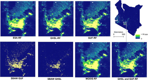
Qualitatively, the gridded population data sets produced using different models and different built land cover datasets are quite different (Figure 3). The nature of the BD technique produces a distinctly different spatial depiction with population distributions (Figure 4) concentrated in built-only pixels, where all built pixels within a single enumeration area will have the same estimated number of people present since each built pixel within a single census unit is expected to have the same population density. In contrast, comparing across the five RF-based models, population counts are distributed across larger areas and at much larger ranges of population densities. The most detailed RF-based outputs are those that include GUF and GHSL settlement areas (Figure 4), which have nominal spatial resolutions much finer than either the MODIS or ESA products.

Figure 4. Qualitative comparison of the seven population models. The maps highlight population patterns (people per pixel (ppp)) for Nairobi and the surrounding area of Kenya at ∼100 m spatial resolution with increasingly yellow shaded pixels representing higher counts. Model descriptions provided in the methods section.

3.2. Random Forest model results

For each RF model, an assessment of variable importance is produced and provides a means to evaluate the relative importance of different covariates included in the model. An example is given for the GUF + GHSL, combined RF-model (Figure 5) which shows ten covariates ranked by importance. Variables that were consistently strong predictors are visualized by country and region. Gaps that exist in the rankings include covariates not plotted in this covariate list. For the GUF + GHSL RF model, the GUF variable consistently ranks as one of the most important variables across all countries and regions as measured by its effect on model fit. This effect is measured by the percentage RMSE increase when that covariate is randomly reassigned to observations in the out-of-bag sample (refers to observations randomly withheld for validation, and different for each tree) (Breiman 2001) and then population density is re-predicted. Other patterns are present, but highly variable between countries and regions, showing that variable importance rankings may be unstable between countries and should be interpreted with caution. Variable importance measures for random forests in general are known to be unstable between models and even resampled data when covariates are highly correlated (Liaw and Wiener 2002; Calle and Urrea 2011). Therefore, raw variable importance metrics in population modeling (e.g. % increase in MSE) are less useful for variable selection and inference, and the more stable rankings are preferred, though still unstable (Nieves et al. 2017). For comparison, raw variable importance in terms of increase in MSE are presented in Supplementary Information S1.

Figure 5. Variable importance plot for the GUF + GHSL Random Forest model with a rank of 1 being most important. The top ten covariates in terms of variable importance as ranked by percentage increase in RMSE when that variable was randomly reassigned to out-of-bag data. These scores were ranked by country and separated by region. DT and DTE refer to distance-to and distance-to-edge respectively. In bold are the three built land cover representations included in the GUF + GHSL RF model.

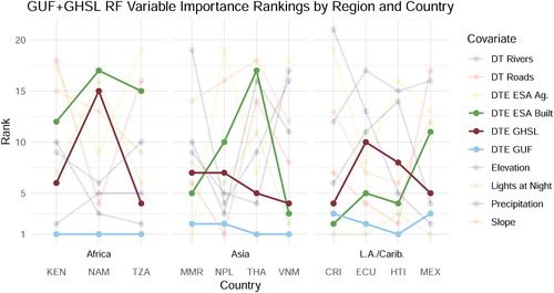
While Figure 5 presents results for only the model with all built data included, GUF consistently performed as one of the top three variables of importance when included in the modeling framework for all countries on its own. Other built data were not as consistent in these single-built area models, and in certain cases other covariates may have more influence on the prediction density weightings.

3.3. Model assessments

Gridded population estimates that were constructed using coarser scale administrative units were summed and compared to units from the finest level available for each country and deviations for these validation units quantified using several different metrics. Tables 1–3 contain the quantitative comparisons of model fit to sampled validation data. Statistical metrics presented for each model include root mean square error (RMSE), percent RMSE (calculated as RMSE divided by the average population density of the sampled validation units, times 100), and mean absolute error (MAE). Validation units represent the number of administrative units used for the validation assessment in each model. Figure 6 shows a comparison across all models for each country with mean absolute error of population density (MAE density), which conditions this metric on administrative unit area.

Figure 6. Model fit compared by mean absolute error of validation units for each country modeled using either a Random Forest-based approach (ESA, GHSL, GUF, GUF/GHSL and MODIS) or a simple binary dasymetric (BD), areal weighting approach (SBAW GHSL, SBAW GUF).

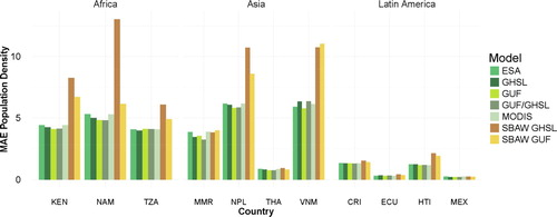
Table 1. Description of main predictive covariates and ancillary data used in population disaggregation methods. The built land covers are input for models of the binary dasymetric method.

Predictive Covariates	Description/Source	Data Type/Nominal Resolution	Reference
Land Cover Types (excluding Built)
Cultivated terrestrial lands	ESA CCI land cover v 2.0, distance to outer edge calculated for each land cover class	Rasters, 10 arc seconds	ESA (2017)
Woody/Trees
Shrubs
Herbaceous
Other terrestrial veg.
Aquatic veg.
Urban area
Bare area
Water
Built Land Covers
Urban Land Class	MERIS-derived, ESA CCI land cover	15 arc-second	ESA (2017)
Global Urban Footprint (GUF)	DLR Earth Observation Center	78 m	Esch et al. (2014)
Global Human Settlement Layer (GHSL)	European Commission, Joint Research Centre (JRC)	38 m	Pesaresi et al. (2016)
MODIS Urban Extent	Distance-to-urban, 2000–2001	500 m	(Schneider, Friedl, and Potere (2009)
Other Datasets
Nighttime Lights	Suomi VIIRS-Derived, 2012	15 arc-second	Elvidge et al. (2013)
Mean temperature, 1950–2000	WorldClim, 1950–2000	30 arc-second	Fick and Hijmans (2017)
Mean precipitation, 1950–2000	WorldClim, 1950–2000	30 arc-second	Fick and Hijmans (2017)
Protected Areas	WDPA, IUCN 2012, distance-to		IUCN and UNEP (2012)
Elevation, SRTM	HydroSHEDS, 2000	3 arc-second	Lehner et al. (2006)
Derived Slope
Roads	Open Street Map, 2017, distance-to	100 m	OSM (2017)
Waterbodies
Rivers

Table 2. Statistical metrics for population density, Asian countries.

ISO	Model	RMSE	% RMSE	MAE
Myanmar (MMR) Validation Units: 210	ESA-RF	16.12	95.43	3.85
	MODIS-RF	16.54	97.91	3.88
	GHSL-RF	14.63	86.78	3.44
	GUF-RF	15.1	89.14	3.54
	GUF and GHSL-RF	13 . 97	82.87	3.23
	BD GHSL	17.28	103.18	3.82
	BD GUF	19.13	114.21	4
Vietnam (VNM) Validation Units: 312	ESA-RF	20.51	77.33	5.91
	MODIS-RF	20.58	77.6	6.12
	GHSL-RF	21.4	80.72	6.34
	GUF-RF	19.95	75.25	5.78
	GUF and GHSL-RF	21.37	80.6	6.36
	BD GHSL	31.96	126.51	10.74
	BD GUF	37.63	148.98	11.03
Nepal (NPL) Validation Units: 355	ESA-RF	26.3	233.96	6.16
	MODIS-RF	26.25	233.51	6.16
	GHSL-RF	26.21	232.24	6.07
	GUF-RF	25.24	223.63	5.81
	GUF and GHSL-RF	25.31	224.25	5.85
	BD GHSL	38.21	332.65	10.71
	BD GUF	28.56	248.68	8.59
Thailand (THA) Validation Units: 380	ESA-RF	4.3	104.93	0.87
	MODIS-RF	4.28	104.63	0.86
	GHSL-RF	4.14	101.24	0.82
	GUF-RF	3.87	94.43	0.75
	GUF and GHSL-RF	3.95	96.56	0.76
	BD GHSL	3.84	98.17	0.92
	BD GUF	3.94	100.85	0.82

Table 3. Statistical metrics for population density, Latin American countries.

ISO	Model	RMSE	% RMSE	MAE
Haiti (HTI) Validation Units: 380	ESA-RF	4.46	88.87	1.24
	MODIS-RF	4 . 05	80.83	1.17
	GHSL-RF	4.52	90.2	1.23
	GUF-RF	4.33	86.33	1.17
	GUF and GHSL-RF	4.48	89.36	1.18
	BD GHSL	7.44	149.24	2.13
	BD GUF	7.42	148.83	1.92
Ecuador (ECU) Validation Units: 652	ESA-RF	1.41	117.03	0.31
	MODIS-RF	1.37	113.74	0.30
	GHSL-RF	1.50	124.14	0.35
	GUF-RF	1.43	118.82	0.31
	GUF and GHSL-RF	1.49	123.43	0.32
	BD GHSL	1.15	95.62	0.42
	BD GUF	1.60	132.99	0.36
Costa Rica (CRI) Validation Units: 312	ESA-RF	4.01	44.92	1.33
	MODIS-RF	3.93	44.04	1.32
	GHSL-RF	3.86	43.26	1.31
	GUF-RF	3.96	44.42	1.31
	GUF and GHSL-RF	3.84	42.97	1.29
	BD GHSL	4.39	49.16	1.52
	BD GUF	4.36	48.77	1.41
Mexico (MEX) Validation Units: 1638	ESA-RF	1.25	65.68	0.24
	MODIS-RF	1.26	66.16	0.25
	GHSL-RF	0.99	52.11	0.22
	GUF-RF	1.01	52.80	0.22
	GUF and GHSL-RF	0.94	49.45	0.21
	BD GHSL	0.72	37.74	0.24
	BD GUF	0.75	39.20	0.23

For seven of the 11 countries tested, RF models do as well or better than BD models based on the comparison metrics performed. Conversely, for four of 11 countries BD models do as well or better than RF models, where it should be noted that though the smallest metric is highlighted for each type, these can be inherently noisy estimates due to random sampling of validation units and small differences should be ignored. Such small differences are observed in a few countries (MEX, MMR, THA). Focusing on the GHSL and GUF data within each country, and in its most direct comparison the metrics for only BD models, we see that GHSL BD models do as well or better than GUF BD in six of 11 countries, based on RMSE. This highlights that it is not only the strengths of association between built areas and population density that varies between countries, but that disagreements between built area data sets can have impacts in their derived uses.

Using assessment data for Kenya, Figure 7 plots observed versus predicted population densities for validation units across each model type, RF- and BD-based (other countries are presented as Supplementary Data S2). A log scale is used to keep values constrained and visible on a single plot. Each point plotted represents the error for a given administrative unit from the two-thirds of units in the finest census data used to calculate validation metrics. Across the different RF-based models (Figure 7(a–e)) we observe the tendency to over predict in units with lower population densities and underpredict in units with high population densities, as observed in the tails and scatter of the units above the 1:1 line below 100 people/km². With BD models (Figure 7(f–g)) we observe that without the benefit of other covariates predictions are more spread around the 1:1 line, which is reflected in all of the validation metrics calculated for Kenya (Table 4, Figure 6) and results in a larger 25th density percentile boundary. In general larger deviations between observed and predicted values for BD models are producing worse statistical metrics of fit for most countries (Figure 5, Tables 2–4).

Figure 7. Comparison of estimations with observed population density in Kenyan validation units by model type. Other countries validation results are presented in Supplementary Data S2. Each panel shows the log population density in people/km² for two thirds of census units used in validation (N = 3358, see Section 2.4 for model acronym explanations). Because of the log scale zeroes are not included on the charts though they affect density percentiles, point, and bootstrapped statistic estimates (Figure 8, Tables 2–4, S3).

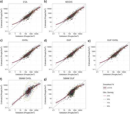
Table 4. Statistical metrics for population density, African countries.

ISO	Model	RMSE	% RMSE	MAE
Kenya (KEN) Validation Units: 3358	ESA-RF	27.37	225.79	4.41
	MODIS-RF	27.35	225.67	4.41
	GHSL-RF	26.04	215.13	4.24
	GUF-RF	24 . 53	202.59	4.08
	GUF and GHSL-RF	25.16	207.84	4.12
	BD GHSL	31.26	257.69	8.26
	BD GUF	34.07	280.91	6.7
Namibia (NAM) Validation Units: 3650	ESA-RF	19.85	98.09	5.31
	MODIS-RF	19.8	97.83	5.29
	GHSL-RF	15.68	79.45	5.00
	GUF-RF	15.15	77.22	4.82
	GUF and GHSL-RF	15.15	77.22	4.81
	BD GHSL	38.7	191.19	13.03
	BD GUF	23.72	117.18	6.14
Tanzania (TZA) Validation Units: 4937	ESA-RF	40.94	300.55	4.07
	MODIS-RF	40.78	299.37	4.07
	GHSL-RF	40.79	299.98	3.97
	GUF-RF	39.73	291.67	4.11
	GUF and GHSL-RF	40.46	297.08	4.08
	BD GHSL	33.62	255.27	6.08
	BD GUF	30.19	229.21	4.91

3.4. Bootstrap model comparison

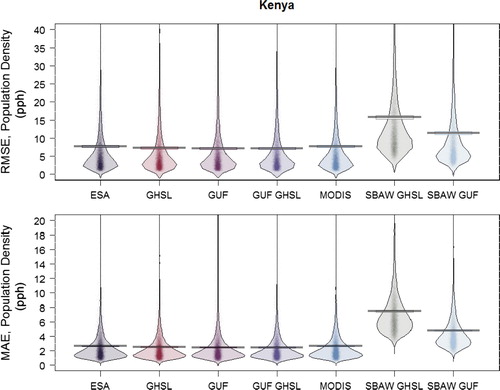
We present a bootstrapped version of results for both RMSE and MAE for Kenya in Figure 8 using ‘pirate plots,’ a boxplot alternative, similar to beanplots (Kampstra 2008; Phillips 2017). On the x-axis are the various models, each with a different built-area data source or combination of data and model type labeled. The raw data (i.e. 10,000 validation samples from the finest available data with each metric calculated for each sample) are plotted as points, with their densities distributed along the y-axis. By using a bootstrapped sample, the modality of each model comparison metric and its variability becomes more visible within the country. The variability validation metrics for Kenya is not as extreme as it might be with a country that has a lower overall proportion of original validation units from which we would sample to generate these plots. Since Kenya has a large sample of validation units (n = 3358), we expect less variation around the point estimates for both RMSE and MAE. Variation in these validation metrics is important and illustrates how sensitive these point-based estimates of model fit might be to random sampling of administrative units. Despite that variation there is still a noticeable difference between the RF outputs and the BD models for Kenya, with stronger model performance for all RF models, whether measured by RMSE or MAE metrics. Bootstrapped plots for all countries are included in the Supplementary Information S1, figures 1-10.

Figure 8. The results by model type for Kenya are shown for (a) RMSE and (b) MAE metrics as calculated on population densities of validation units (people per hectare). Different models with different built representations are shown on the x-axis. The colored points represent individual raw data values while the horizontal lines indicate the central tendencies for each model. The first five models are Random Forest-based while the last two are based on the simple binary areal weighting (BD) approach.

4. Discussion

4.1. Summary of results

Deepening our understanding of how remotely-sensed representations of built-areas are integrated into population modeling efforts is paramount to successful production of accurate, reliable gridded population maps, especially in low and middle-income countries where census data may be coarser and less updated. We have addressed significant questions about the relative utility of several of these or their proxies (ESA/MERIS land cover, GUF, GHSL, and MODIS-derived) in the specific context of gridded human population modeling of eleven countries in the Global South. The results from these analyses can be presented in two key statements:

The differences between the built-area data products tested produce both qualitative and quantitative differences in gridded population estimates.

For the countries tested, multiple built-area data sources included as covariates in a weighted disaggregation tends to outperform models with fewer, and in seven out of 11 countries is better than relying on binary disaggregation into built area extents.

Our ability to remotely sense and classify built-areas on the Earth's surface at increasingly larger extents and finer grains is facilitating the use of such products in new ways. And though the results from this study are not expected to be globally representative, the insights we gain from analyses in these eleven case study countries show that relying solely on one built-area product may expose derived outputs to any limitations in those products. This suggests that approaches that incorporate more than one built-area data set, such as the RF-based population modeling conducted here, may benefit from the relative values of each product while minimizing to some extent the impacts of individual misclassifications.

4.2. Choice of built land cover classifications in gridded population models

The limitations of global built-area products usually fall broadly into the category of misclassification errors due to under- or over-specificity of the classification scheme employed. These classification systems vary by product, and necessarily with the spatial, sensor, and temporal characteristics of the data used to derive them. Referring to Figure 2 it is unsurprising to see differences in these built-area estimates for a large urban core as their inherent ability to detect built-areas across different mixtures of urban/suburban vegetation is quite different (Esch et al. 2014; Pesaresi et al. 2015; Esch et al. 2013; Pesaresi et al. 2016).

These differences between products and the data used to derive them are particularly important in applications where urban and rural built-areas differ considerably. In many developing contexts built, settled areas likely have structures that are very low-lying relative to surrounding vegetation, etc. and active-sensor derived products may actually misclassify these regions more readily than moderate or high-resolution optical products. In our study, population mapping relies very much on getting classification accuracies right in both of these contexts. This is exacerbated when disaggregating population only to built-classified pixels (e.g. BD models). If a structure or built-area is not detected, then it will receive a zero weighting, and any misclassification resulting in predicting no population in a particular area may be quite undesirable (e.g. vaccination planning, disaster relief, etc.). Conversely, as shown in those countries where BD models outperformed the more complex models, at least in terms of RMSE (THA, ECU, MEX and TZA), when built area data is accurate and proportionally coherent with population density then the added complexity of building a weighting model may be unnecessary or perhaps even detrimental. Unfortunately, being limited to conducting coarsening/disaggregation model comparison, with a lack of spatially explicit and independent validation we still cannot assess overall levels of model uncertainty in a way that is not constrained by census data used in the analysis.

4.3. Binary vs. multivariate, weighted dasymetric approach

When the RF modeling approach is used, GUF and GHSL both change the qualitative, visual outcome of the mapping. However, GUF tends to do so more than GHSL, likely due to its higher RF model variable importance. GUF is also usually associated with improvements in validation metrics for models it is included in (Tables 2–4). The fact that the GUF product is partially derived from non-optical information suggests that GUF and other non-optical, remotely sensed data can complement data derived from other remotely sensed information. Therefore, improvements in built area data, such as the newer S1 GHSL effort which combines Sentinel 1A Earth Observation data in its classification algorithm to improve in built-up area detection over the original GHSL Landsat data are extremely important (Corbane et al. 2017). Findings from this study support the conclusion that including multiple built-area covariates in the RF model may improve model results, and points to the need for a more broad and in-depth study across more developed contexts as to when and how multiple built-area data sets can improve more complex, gridded population models. This is particularly interesting given the previous discussion about the relatively high disagreement between all of these products.

While simpler to apply, the BD approach and its errors are purely constrained by the two sources of data driving the gridded estimates: the census and the built area data. The production of the built data alone can involve various sources of complexity such as multiple sensors and algorithms (e.g. Pesaresi et al. 2015) so consideration needs to be given to how the underlying settlement data are generated and where its sources of errors are coming from. Concentrating population into areas defined as ‘built’ may work well with the BD approach in highly developed regions where optical or radar-based approaches both provide strong agreement between the built signal and actual settled land cover (Merkens and Vafeidis 2018). It is also with great interest that higher resolution data products, such as those derived via machine learning approaches and sub-five-meter imagery are now being developed, albeit not at global extents. These types of data have already been used to estimate population counts such as with the Facebook High Resolution Settlement Layer (HRSL) (Facebook Connectivity Lab and Columbia University Center for International Earth Science Information Network 2017).

Beyond their use in BD type redistributions like HRSL, very high-resolution data offers to resolve individual structures, which can be further classified into residences vs. non-residences, not just built/non-built, or aggregated built area density. With better data sources, combinations of different sensor types, and perhaps data fusions that include temporality as longer periods of time are covered with data at global scales, we may have the opportunity to not just classify built vs. non-built, but extract information about the quality and structure of the built-environment. This trend is analogous to that which we have observed in the land change community and applications expanding to include remote sensing of land use and land conditions instead of focusing strictly on land cover change.

4.4. Spatial modeling considerations for gridded population datasets

Affecting both types of disaggregation approaches presented here, the resolution of the input census data also will strongly drive the robustness of the RF model. Fine-scaled, highly detailed census units will improve the RF model due to the increased spatial specificity and range of variability in population density for which the model is trained. This in turn will improve predictions of the dasymetric weighting layer because the scalar disconnect between model and pixel-level predictions will decrease. Critically, however, any error introduced at the level of the census data collection will propagate through the model and reflect in the final output. Thus, gridded population products for countries that have detailed, accurate, current census data will almost always provide a more robust final output than others, regardless of whether you use a multivariate model like RF or a lightly-modeled approach like BD, and this has implications as the next round of decadal censuses are produced, which may offer up new and more detailed data that may change the relative merits of simple and complex gridded disaggregation techniques.

It should also be noted that built land cover data is not the only type of covariate that correlates well with population distribution and densities (Stevens et al. 2015; Sorichetta et al. 2015). The non-linear, nonparametric nature of the RF approach provides a framework to better integrate various types of discrete and continuous information that informs the prediction density estimation. This can be a more robust approach than relying on one built land cover product alone for redistribution population counts as that built land cover product comes with its own inherent error and bias for what is identified as ‘built’ on the landscape. In addition, the type of built-area may or may not be coincident with residential populations (e.g. commercial/industrial versus residential settlement). This explains why in some models other covariates might supercede built areas data in their variable importance, especially when those built areas may be inherently difficult to classify.

There may be additional factors that influence the distribution and density of population for various built land covers which may not be captured by either the RF or the BD modeling approach. The dasymetric component of these two models is considered a ‘top-down’ type of modeling effort, which relies on the accuracy of the underlying built data and also the granularity of the input administrative units for accurately redistributing populations. For example, alternatives to creating population estimates from census data are to by-pass the use of census data altogether, relying instead on remotely-sensed proxies at relatively high resolutions that correlate well with population and model it in a more bottom-up approach (Bharti et al. 2016; Tatem 2014).

For those seven countries where the RF approach outperforms the BD approach, there is consensus that GUF is a stronger predictor than other built data, but not always. This suggests that even with increasing spatial resolution of globally available built land cover datasets, a modeling approach that integrates other covariates that co-vary with population distribution and may still offer advantages from additional explanatory power. In addition, while the quantitative differences across models vary in magnitude, there is a visible, qualitative difference between gridded population estimates, which is driven by the underlying data used as covariates and how those data are incorporated (or not) to produce a final, gridded population dataset.

Future work should include testing, and further validation of these approaches using systematic intersections of built-area data sources and population counts at multiple scales and across different development and data quality contexts. Further research should interrogate the relationships we observe in our eleven case study countries globally, especially in areas and countries outside of the Global South. Built area data production and its associations with population density will vary greatly across low to high development and income contexts, and the general trends in modeling outcomes may vary from country to country.

Considerations should be given to the inclusion of census data to model population distributions and densities or if other, more contemporary approaches may be appropriate which take advantage of high resolution remotely-sensed data or other crowd-sourced types of information such as tweets or mobile phone call records (Patel et al. 2016; e.g. Deville et al. 2014). These other techniques that rely on crowd-sourced information to model population distributions and movements come with their own significant sources of error but offer potential for mapping at finer temporal grains than traditional decadal census data (Hughes et al. 2016) and may be used to address population movements. In addition, the coupling of remotely-sensed data with mobile phone records is becoming more tractable with increased accessibility and continued spatial and temporal refinement of all datasets (Steele et al. 2017). Furthermore, understanding and leveraging the differences between remotely-sensed built-areas is encouraged. For example, built-up areas, as better measured by active sensing technologies like synthetic aperture radar (e.g. GUF), differ in their relation to residential population when compared with just built-area or impervious surfaces as derived from multispectral data (e.g. GHSL/Landsat, ENVISAT MERIS, or MODIS). And increasingly, derived remote-sensing products are combining optical- and radar-based data to produce improved representations of not just built-areas but built-volumes, globally, and at increasingly fine-scale resolutions. These advances are further pushing our ability to detect and attribute places on the surfaces of the Earth to not just human-used, but increasingly finer grained classification of that use. Therefore, as longer time series and greater extents of the Earth's surface are imaged using newer sensors, and we have a greater variety of ways of characterizing and sub-classifying the built environment from remotely sensed data, we should continue to refine their integration into population modeling.

5. Concluding comments

The improvement in high-resolution satellite-based products continues to increase with the advancements of different computer-based algorithms and the capability of dealing with high dimensional and multi-dimensional datasets at larger and larger extents. As a result, there is an increasingly valuable pool of data products informing population maps. Providing a framework that can take advantage of the strengths of these different data products in a multivariate way, potentially leveraging their strengths and minimizing each product's inherent inaccuracies is highly desirable. Our results highlight one such method based on the machine learning, Random Forest-based approach for population modeling. Relying only on one built land cover dataset to redistribute population counts assumes that underlying land cover product is accurate in all contexts, directly reflects residential conditions, and that the redistribution within the built land cover pixels should be uniform within enumeration areas. This is rarely realistic, but does not necessarily obviate the utility of simple, consistent approaches. We argue that the intersection between modeling approach and the strengths and limitations of the various sources of data will determine the overall generalizability of any population modeling effort. Based on our results, it remains unclear that there is a one-size-fits-all solution on the spectrum from extreme simplicity in dasymetric redistribution to relatively complex models like RF. Nor do our results indicate that a single built area data source may be generally more accurate or useful than any other in any one population modeling context. Both GHSL and GUF perform better than the other in BD models in at least a few cases as measured by RMSE or MAE, indicating that either may be more strongly associated with population density in varying contexts, and that testing across contexts is needed.

Gridded population datasets and how different built area data inform them is an important research intersection. Gridded population data provide baseline denominator information for modeling and application efforts globally. There are increasingly more options for choosing across high resolution, remotely-sensed data products and the integration of these multiple data products can further the advances of how these base denominator datasets get produced. For data poor environments, where ancillary data are rare, built areas or their density are very often the most important predictors of human population. Increasingly, these data are being used in bottom-up predictions of population, and insights gained about which built data relate the best, across varying contexts and remote sensing characteristics is critical. Findings from this study highlight that further effort is needed to understand how errors inherent in different built land cover products for more or less populated areas (e.g. urban versus rural) subsequently influence the modeling process, whether lightly modeled or from a more complex statistical process.

Acknowledgements

We would like to acknowledge previous reviews and editorial comments which have improved the manuscript prior to its submission to IJDE.

Disclosure statement

No potential conflict of interest was reported by the authors.

ORCID

Forrest R. Stevens http://orcid.org/0000-0002-9328-3753

Additional information

Funding

FRS, AEG, JNN, AK, and AS are funded by the Bill & Melinda Gates Foundation (OPP1134076). AJT is supported by funding from U.S. National Institutes of Health/National Institute of Allergy and Infectious Diseases (U19AI089674), the Bill & Melinda Gates Foundation (OPP1106427, OPP1032350, OPP1134076), the Clinton Health Access Initiative, National Institutes of Health, and a Wellcome Trust Sustaining Health Grant (106866/Z/15/Z).

References

- Anderson, D. E., and P. N. Anderson. 1973. “Population Estimates by Humans and Machines.” Photogrammetric Engineering 39 (2): 147–154. http://trid.trb.org/view.aspx?id=92581.
- Azar, Derek, Ryan Engstrom, Jordan Graesser, and Joshua Comenetz. 2013. “Generation of Fine-Scale Population Layers Using Multi-Resolution Satellite Imagery and Geospatial Data.” Remote Sensing of Environment 130 (March): 219–232. doi:10.1016/j.rse.2012.11.022.
- Azar, Derek, Jordan Graesser, Ryan Engstrom, Joshua Comenetz, Robert M. Leddy, Nancy G. Schechtman, and Theresa Andrews. 2010. “Spatial Refinement of Census Population Distribution Using Remotely Sensed Estimates of Impervious Surfaces in Haiti.” International Journal of Remote Sensing 31 (21): 5635–5655. doi:10.1080/01431161.2010.496799.
- Balk, Deborah L., Uwe Deichmann, Greg Yetman, Francesca Pozzi, Simon I. Hay, and Andy Nelson. 2006. “Determining Global Population Distribution: Methods, Applications and Data.” Advances in Parasitology 62 (January): 119–156. doi:10.1016/S0065-308X(05)62004-0.
- Balk, Deborah L., and Greg Yetman. 2004. The Global Distribution of Population: Evaluating the Gains in Resolution Refinement. New York: Center for International Earth Science Information Network (CIESIN). http://sedac.ciesin.org/gpw/docs/gpw3_documentation_final.pdf.
- Barber, G. M. 1988. Elementary Statistics for Geographers. New York: Guilford Press.
- Bhaduri, Budhendra, Edward Bright, Phillip R. Coleman, and Marie L. Urban. 2007. “LandScan USA: a High-Resolution Geospatial and Temporal Modeling Approach for Population Distribution and Dynamics.” GeoJournal 69 (1/2): 103–117. http://connection.ebscohost.com/c/articles/27560012/landscan-usa-high-resolution-geospatial-temporal-modeling-approach-population-distribution-dynamics. doi: 10.1007/s10708-007-9105-9
- Bharti, Nita, Ali Djibo, Andrew J. Tatem, Bryan T. Grenfell, and Matthew J. Ferrari. 2016. “Measuring Populations to Improve Vaccination Coverage.” Scientific Reports 6 (1): 34541. doi:10.1038/srep34541.
- Bivand, Roger S., Tim Keitt, and Barry Rowlingson. 2017. “Rgdal: Bindings for the Geospatial Data Abstraction Library.” https://cran.r-project.org/package=rgdal.
- Bontemps, S., P. Defourny, E. V. Bogaert, O. Arino, V. Kalogirou, and J. R. Perez. 2011. “GLOBCOVER 2009 - Products Description and Validation Report.” European Space Agency.
- Breiman, Leo. 2001. “Random Forests.” Machine Learning 45 (1): 5–32. doi:10.1023/A:1010933404324.
- Calle, M. Luz, and Víctor Urrea. 2011. “Letter to the Editor: Stability of Random Forest Importance Measures.” Briefings in Bioinformatics 12 (1): 86–89. doi:10.1093/bib/bbq011.
- CIESIN. 2017. Gridded Population of the World, Version 4 (GPWv4): Population Count. New York: Center for International Earth Science Information Network, Columbia University. doi:10.7927/H4X63JVC.
- Corbane, Christina, Martino Pesaresi, Panagiotis Politis, Vasileios Syrris, Aneta J. Florczyk, Pierre Soille, Luca Maffenini, et al. 2017. “Big Earth Data Analytics on Sentinel-1 and Landsat Imagery in Support to Global Human Settlements Mapping.” Big Earth Data 1 (1–2): 118–144. doi:10.1080/20964471.2017.1397899. Taylor & Francis.
- Deville, Pierre, Catherine Linard, Samuel Martin, Marius Gilbert, Forrest R. Stevens, Andrea E. Gaughan, Vincent D. Blondel, and Andrew J. Tatem. 2014. “Dynamic Population Mapping Using Mobile Phone Data.” Proceedings of the National Academy of Sciences 111 (45): 15888–15893. doi:10.1073/pnas.1408439111.
- Dobson, Jerome E., Edward A. Brlght, Phillip R. Coleman, and Brian A. Worley. 2000. “LandScan: A Global Population Database for Estimating Populations at Risk.” Photogrammetric Engineering & Remote Sensing 66 (7): 849–857.
- Doxsey-Whitfield, Erin, Kytt MacManus, Susana B. Adamo, Linda Pistolesi, John Squires, Olena Borkovska, and Sandra R. Baptista. 2015. “Taking Advantage of the Improved Availability of Census Data: A First Look at the Gridded Population of the World, Version 4.” Papers in Applied Geography, doi:10.1080/23754931.2015.1014272.
- Eicher, Cory L., and Cynthia A. Brewer. 2001. “Dasymetric Mapping and Areal Interpolation: Implementation and Evaluation.” Cartography and Geographic Information Science 28 (2): 125–138. doi:10.1559/152304001782173727.
- Elvidge, Christopher D., Kimberly E. Baugh, Mikhail Zhizhin, and Feng-Chi Hsu. 2013. “Why VIIRS Data Are Superior to DMSP for Mapping Nighttime Lights.” Proceedings of the Asia-Pacific Advanced Network, 62–79. doi:10.7125/APAN.35.7.
- ESA. 2017. Land Cover CCI Product User Guide Version 2.0. Europeah Space Agency (ESA). http://maps.elie.ucl.ac.be/CCI/viewer/download/ESACCI-LC-Ph2-PUGv2_2.0.pdf.
- Esch, T., M. Marconcini, A. Felbier, A. Roth, W. Heldens, M. Huber, M. Schwinger, H. Taubenbock, A. Mueller, and S. Dech. 2013. “Urban Footprint Processor—Fully Automated Processing Chain Generating Settlement Masks From Global Data of the TanDEM-X Mission.” IEEE Geoscience and Remote Sensing Letters 10 (6): 1617–1621. doi:10.1109/LGRS.2013.2272953.
- Esch, T., M. Marconcini, D. Marmanis, J. Zeidler, S. Elsayed, A. Metz, A. Mueller, and S. Dech. 2014. “Dimensioning Urbanization – An Advanced Procedure for Characterizing Human Settlement Properties and Patterns Using Spatial Network Analysis.” Applied Geography, doi:10.1016/j.apgeog.2014.09.009.
- European Commission Joint Research Centre, and Columbia University Center for International Earth Science Information Network. 2015. “GHS Population Grid, Derived from GPW4, Multitemporal (1975, 1990, 2000, 2015). European Commission, Joint Research Centre (JRC) [Dataset].” European Comission, Joint Research Centre (JRC). http://data.europa.eu/89h/jrc-ghsl-ghs_pop_gpw4_globe_r2015a.
- Facebook Connectivity Lab, and Columbia University Center for International Earth Science Information Network. 2017. “High Resolution Settlement Layer (HRSL).” Facebook Connectivity Lab and Center for International Earth Science Information Network, Columbia University. https://ciesin.columbia.edu/data/hrsl/.
- Farr, T. G. 2007. “The Shuttle Radar Topography Mission.” Reviews of Geophysics 45), doi:10.1029/2005RG000183.
- Fick, Stephen E., and Robert J. Hijmans. 2017. “WorldClim 2: New 1-Km Spatial Resolution Climate Surfaces for Global Land Areas.” International Journal of Climatology, doi:10.1002/joc.5086.
- Florczyk, A. J., M. Melchiorri, J. Zeidler, C. Corbane, M. Schiavina, S. Freire, F. Sabo, P. Politis, T. Esch, and M. Pesaresi. 2019. “The Generalised Settlement Area: Mapping the Earth Surface in the Vicinity of Built-up Areas.” International Journal of Digital Earth 0 (0): 1–16. doi:10.1080/17538947.2018.1550121. Taylor & Francis.
- Fotheringham, A. Stewart, and Peter A. Rogerson. 1993. “GIS and Spatial Analytical Problems.” International Journal of Geographical Information Systems 7: 3–19. doi: 10.1080/02693799308901936
- Freire, Sergio, Kytt McManus, Martino Pesaresi, Erin Doxey-Whitfield, and Jane Mills. 2016. “Development of New Open and Free Multi-Temporal Global Population Grids at 250 m Resolution.” In Proceedings of the 19th AGILE conference on geographic information science, June 14–17, Helsinki, Finland.
- Frye, C., E. Nordstrand, and Environmental Systems Research Institute. 2017. Documentation for the World Population Estimated (WPE) Data Set. Redlands, CA: ESRI.
- Gaughan, Andrea E., Forrest R. Stevens, Zhuojie Huang, Jeremiah J. Nieves, Alessandro Sorichetta, Shengjie Lai, Xinyue Ye, et al. 2016. “Spatiotemporal Patterns of Population in Mainland China, 1990 to 2010.” Scientific Data 3 (February): 160005. doi:10.1038/sdata.2016.5. Macmillan Publishers Limited.
- Gaughan, Andrea E., Forrest R. Stevens, Catherine Linard, Peng Jia, and Andrew J. Tatem. 2013. “High Resolution Population Distribution Maps for Southeast Asia in 2010 and 2015.” PLOS ONE 8 (2): e55882. doi:10.1371/journal.pone.0055882.
- Gaughan, Andrea E., Forrest R. Stevens, Catherine Linard, Nirav N. Patel, and Andrew J. Tatem. 2014. “Exploring Nationally and Regionally Defined Models for Large Area Population Mapping.” International Journal of Digital Earth, 1–18. doi:10.1080/17538947.2014.965761.
- GDAL Development Team. 2016. “GDAL – Geospatial Data Abstraction Library, Version 2.1.0.” Open Source Geospatial Foundation. http://www.gdal.org.
- Grekousis, George, Giorgos Mountrakis, and Marinos Kavouras. 2015. “An Overview of 21 Global and 43 Regional Land-Cover Mapping Products.” International Journal of Remote Sensing, doi:10.1080/01431161.2015.1093195.
- Hijmans, Robert J., Susan E. Cameron, Juan L. Parra, Peter G. Jones, and Andy Jarvis. 2005. “Very High Resolution Interpolated Climate Surfaces for Global Land Areas.” International Journal of Climatology 25 (15): 1965–1978. doi:10.1002/joc.1276.
- Hijmans, Robert J., and Jacob Van Etten. 2012. “Package ‘Raster.’” http://raster.r-forge.r-project.org/.
- Hughes, Christina, Emilio Zagheni, Guy J. Abel, Alessandro Sorichetta, Arkadius Wi’sniowski, Ingmar Weber, and Andrew J. Tatem. 2016. Inferring Migrations: Traditional Methods and New Approaches Based on Mobile Phone, Social Media, and Other Big Data: Feasibility Study on Inferring (Labour) Mobility and Migration in the European Union From Big Data and Social Media Data. Luxembourg: European Union. https://eprints.soton.ac.uk/408499/.
- IUCN and UNEP. 2012. The World Database on Protected Areas (WDPA). Cambridge: UNEP-WCMC. http://www.protectedplanet.net.
- Kampstra, Peter. 2008. “Beanplot: A Boxplot Alternative for Visual Comparison of Distributions.” Journal of Statistical Software 28: 1–9. http://www.jstatsoft.org/v28/c01/paper. doi: 10.18637/jss.v028.c01
- Lehner, Berhnard, Kris Verdin, Andy Jarvis, and World Wildlife Fund. 2006. HydroSHEDS Technical Documentation. World Wildlife Fund. http://www.worldwildlife.org/freshwater/pubs/HydroSHEDS_TechDoc_v10.pdf.
- Liaw, Andy, and Matthew Wiener. 2002. “Classification and Regression by RandomForest.” R News 2 (3): 18–22. http://cran.r-project.org/doc/Rnews/.
- Linard, Catherine, Victor A. Alegana, Abdisalan M. Noor, Robert W. Snow, and Andrew J. Tatem. 2010. “A High Resolution Spatial Population Database of Somalia for Disease Risk Mapping.” International Journal of Health Geographics 9 (January): 45. doi:10.1186/1476-072X-9-45.
- Linard, Catherine, Marius Gilbert, and Andrew J. Tatem. 2010. “Assessing the Use of Global Land Cover Data for Guiding Large Area Population Distribution Modelling.” GeoJournal 76 (5): 525–538. doi:10.1007/s10708-010-9364-8.
- Lo, C. P. 1995. “Automated Population and Dwelling Unit Estimation From High-Resolution Satellite Images: A GIS Approach.” International Journal of Remote Sensing 16 (1): 17–34. doi:10.1080/01431169508954369. Taylor & Francis.
- Mennis, Jeremy. 2003. “Generating Surface Models of Population Using Dasymetric Mapping.” The Professional Geographer 55 (1): 31–42.
- Mennis, Jeremy. 2009. “Dasymetric Mapping for Estimating Population in Small Areas.” Geography Compass 3 (2): 727–745. doi: 10.1111/j.1749-8198.2009.00220.x
- Mennis, Jeremy, and Torrin Hultgren. 2006. “Intelligent Dasymetric Mapping and Its Application to Areal Interpolation.” Cartography and Geographic Information Science 33 (3): 179–194. doi:10.1559/152304006779077309.
- Merkens, Jan-Ludolf, and Athanasios T. Vafeidis. 2018. “Using Information on Settlement Patterns to Improve the Spatial Distribution of Population in Coastal Impact Assessments.” Sustainability 10 (9): 3170. doi:10.3390/su10093170. Multidisciplinary Digital Publishing Institute.
- Nieves, Jeremiah J. 2016. “Global Population Distributions and the Environment: Discerning Observed Global and Regional Patterns.” M.S. Thesis, Department of Geography and Geosciences, University of Louisville.
- Nieves, Jeremiah J., Forrest R. Stevens, Andrea E. Gaughan, Catherine Linard, Alessandro Sorichetta, Graeme Hornby, Nirav N. Patel, and Andrew J. Tatem. 2017. “Examining the Correlates and Drivers of Human Population Distributions Across Low-and Middle-Income Countries.” Journal of the Royal Society Interface 14 (137), doi:10.1098/rsif.2017.0401.
- OSM. 2017. “OpenStreetMap The Free Wiki World Map.” OpenStreetMap Contributors, CC-BY-SA.
- Patel, Nirav N., Forrest R. Stevens, Zhuojie Huang, Andrea E. Gaughan, Iqbal Elyazar, and Andrew J. Tatem. 2016. “Improving Large Area Population Mapping Using Geotweet Densities.” Transactions in GIS, doi:10.1111/tgis.12214. Early Access.
- Pesaresi, Martino, Daniele Ehrlich, Aneta J. Florczyk, Sergio Freire, Andreea Julea, Thomas Kemper, Pierre Soille, and Vasileios Syrris. 2015. “GHS Built-up Grid, Derived from Landsat, Multitemporal (1975, 1990, 2000, 2014).” European Comissions, Joint Research Centre. http://data.jrc.ec.europa.eu/dataset/jrc-ghsl-ghs_built_ldsmt_globe_r2015b.
- Pesaresi, Martino, Daniele Ehrlich, Aneta J. Florczyk, Sergio Freire, Andreea Julea, Thomas Kemper, Pierre Soille, and Vasileios Syrris. 2016. Operating Procedure for the Production of the Global Human Settlement Layer From Landsat Data of the Epochs 1975, 1990, 2000, and 2014. Ispra: European Comission Joint Research Centre. doi:10.2788/253582.
- Phillips, Nathaniel. 2017. “Yarrr: A Companion to the e-Book ‘YaRrr!: The Pirate’s Guide to R.’” https://cran.r-project.org/package=yarrr.
- Potere, David, Annemarie Schneider, Shlomo Angel, and Daniel Civco. 2009. “Mapping Urban Areas on a Global Scale: Which of the Eight Maps Now Available Is More Accurate?” International Journal of Remote Sensing 30 (24): 6531–6558. doi:10.1080/01431160903121134.
- Roy, Dulal Chandra, and Thomas Blaschke. 2014. “A Grid-Based Approach for Refining Population Data in Rural Areas.” Journal of Geography and Regional Planning 7 (3): 47–57. doi:10.5897/JGRP2013.0409.
- Schneider, A., Mark A. Friedl, and D. Potere. 2009. “A New Map of Global Urban Extent From MODIS Satellite Data.” Environmental Research Letters 4 (4): 044003. doi:10.1088/1748-9326/4/4/044003.
- Schneider, Annemarie, Mark A. Friedl, and David Potere. 2010. “Mapping Global Urban Areas Using MODIS 500-m Data: New Methods and Datasets Based on ‘Urban Ecoregions.’” Remote Sensing of Environment 114 (8): 1733–1746. doi:10.1016/j.rse.2010.03.003.
- Small, Christopher, and Robert J. Nicholls. 2003. “A Global Analysis of Human Settlement in Coastal Zones.” Journal of Coastal Research 19 (3): 584–599.
- Sorichetta, Alessandro, Graeme M. Hornby, Forrest R. Stevens, Andrea E. Gaughan, Catherine Linard, and Andrew J. Tatem. 2015. “High-Resolution Gridded Population Datasets for Latin America and the Caribbean in 2010, 2015, and 2020.” Scientific Data 2 (150045), doi:10.1038/sdata.2015.45.
- Steele, Jessica E., Pål Roe Sundsøy, Carla Pezzulo, Victor A. Alegana, Tomas J. Bird, Joshua Blumenstock, Johannes Bjelland, et al. 2017. “Mapping Poverty Using Mobile Phone and Satellite Data.” Journal of the Royal Society Interface 14 (127), doi:10.1098/rsif.2016.0690.
- Stevens, Forrest R., Andrea E. Gaughan, Catherine Linard, and Andrew J. Tatem. 2015. “Disaggregating Census Data for Population Mapping Using Random Forests with Remotely-Sensed and Ancillary Data.” PLOS ONE 10 (2): e0107042. doi:10.1371/journal.pone.0107042.
- Sutton, P., D. Roberts, C. Elvidge, and K. Baugh. 2001. “Census From Heaven: An Estimate of the Global Human Population Using Night-Time Satellite Imagery.” International Journal of Remote Sensing 22 (16): 3061–3076. doi:10.1080/01431160010007015. Taylor & Francis.
- Tatem, Andrew J. 2014. “Mapping the Denominator: Spatial Demography in the Measurement of Progress.” International Health, doi:10.1093/inthealth/ihu0575.
- Tobler, Waldo, Uwe Deichmann, Jon Gottsegen, and Kelly Maloy. 1997. “World Population in a Grid of Spherical Quadrilaterals.” International Journal of Population Geography 3: 203–225. doi: 10.1002/(SICI)1099-1220(199709)3:3<203::AID-IJPG68>3.0.CO;2-C
- Willmott, Cort J., Scott M. Robeson, and Kenji Matsuura. 2012. “A Refined Index of Model Performance.” International Journal of Climatology 32 (13): 2088–2094. doi:10.1002/joc.2419.
- Willmott, Cort J., Scott M. Robeson, Kenji Matsuura, and Darren L. Ficklin. 2015. “Assessment of Three Dimensionless Measures of Model Performance.” Environmental Modelling & Software 73 (November): 167–174. doi:10.1016/j.envsoft.2015.08.012.