Evaluation of GOFP over four forest plots using RAMI and UAV measurements

ABSTRACT

Comparison and validation of canopy reflectance (CR) models are two important steps to ensure their reliability. Pure forest plantations are an ideal type of forest for validating CR models because of their simple background and the low variance in the crown structures which are usually assumed to be identical in most CR models. A Geometric Optical Model for Forest Plantations (GOFP) was compared using dataset in two radiation transfer model intercomparison exercise (RAMI) stands and validated using in situ dataset of detailed optical and structural data of two forest plantations in the Saihanba Forestry Center, China. The results show that (1) the tree distributions in stands described by the hypergeometric model in GOFP show good consistencies with the dataset in the two RAMI stands and measurements from the two Saihanba forest stands; and (2) the CRs simulated with GOFP are also compared well in the two RAMI stands and validated with measurements collected with unmanned aerial vehicles in the two Saihanba stands. GOFP shows a better consistency with the CR measurements than those from CR models for natual forestsbecause the tree distribution in forest plantations is described more reasonably in GOFP.

KEYWORDS:

• Validation
• forest plantation
• GOFP
• tree distribution
• BRF
• hypergeometric model

1. Introduction

Comparison and validation are always important steps in model development. The reliability of canopy reflectance (CR) models plays a key role in the retrieval of many plant structural and physiological parameters based on remote sensing data. For example, they are used for estimating the Bidirectional Reflectance Factor (BRF). Geometric optical (GO) models are identified as an important class of CR models. GO models are used to estimate vegetation structural parameters, such as leaf area index (LAI) and clumping index because of their emphasis on vegetation structure and its interaction with the radiative transfer processes in the canopy (Li and Strahler 1985; Nilson and Peterson 1991; Chen and Leblanc 1997; Fan et al., 2014a). Compared with many early radiation transfer models (e.g. SAIL (Verhoef 1984)), GO models are more suitable for simulating CR for discrete objects such as forests. GO models have been actively researched during the last forty years. Cylinder and ellipsoid-shaped crowns have been replaced by cone-shaped and ‘cone + cylinder’ crowns to more reasonably describe the crown structure and to capture apical dominance (Li and Strahler 1992; Chen and Leblanc 1997). The Neyman model has replaced the Poisson model to describe the tree distribution in natural forests and to better quantify patchiness and clustering. A clumping index was added in the GO models to better consider the leaf distribution in a canopy (the Four-Scale model) (Chen and Leblanc 1997; Nilson 1999). Because many trees grow on slopes rather than flat surfaces, some GO models added a slope factor (Geometric-Optical Model for Sloping Terrains (GOST) and Geometric-Optical Model for Sloping Terrains-II (GOST2)) (Fan et al. 2014b, 2015). Recently, the exclusion effect among trees was described quantitatively and a GO model for forest plantation (GOFP) was developed for accurately simulating CR (Geng et al. 2017). In addition to simulating canopy BRF, GO models have also been used to retrieve canopy structure parameters, such as LAI (Deng 2006), clumping index (Chen, Menges, and Leblanc 2005; Pisek and Chen 2007; He et al. 2016), crown closure (Chopping et al. 2008), crown volume (Mottus, Sulev, and Lang 2006) and crown diameter (Zeng et al. 2008, 2009), at the regional and global scale.

The abovementioned GO models were most often validated using multi-angle satellite data, such as MODIS (Fan et al., 2014a; Geng et al. 2017). Unfortunately, the spatial resolutions of these data are usually relatively coarse, leading to many the pixels mixed, especially at large view zenith angles (VZAs). The dataset from two RAdiative transfer Model Intercomparison exercise (RAMI) stands provides a platform for comparing many CR models; the development of multi-angle high-resolution images obtained from unmanned aerial vehicles (UAV) provides a new approach for validating CR models. The Järvselja forest dataset collected from Estonia and compiled in 2007 (Kuusk, Kuusk, and Lang 2009), which includes detailed forest structure and canopy reflectance obtained from satellite and UAV platforms covering three mature forest stands (two of them are mixed forests), is a fine dataset for validating CR models. Many CR models have been validated using the Järvselja forest dataset (Kuusk et al. 2008; Kuusk, Kuusk, and Lang 2009, 2014a; Widlowski et al. 2015). Datasets from pure forest plantations are typically used to validate CR models for at least two reasons: (1) most forest CR models assume that the crown structure (height and radius of the crown) of all the trees in a forest stand is identical or with low variance (e.g. Four-Scale model, GOST2, and GORT (Li, Strahler, and Woodcock 1995)), of which situation is more common in forest plantations than in natural forests; and (2) the background in a forest plantation is usually simple because the forest stands are oftentimes composed of single tree species. However, the tree distribution in forest plantations usually show a completely different pattern from those in natural forests and has not been described quantitatively in most existing CR models. Therefore, it is not entirely sound to validate these CR models designed for natural forests using forest plantation data.

The aims of this study are to compare a GOFP using dataset from two RAMI platform stands and validate it using an in situ dataset of detailed optical and structural data of forest plantations. A GOST2 was used for comparison. Both GO models can simulate forest canopy BRF. GOST2 has been widely used for natural forests, while GOFP, which is based on the former model, has been used to simulate CRs for forest plantations with special consideration of the exclusion effect between trees.

2. Study area and dataset

2.1. Saihanba Forestry Center

The field dataset was collected in Saihanba Forestry Center in the summer of 2019, which has the largest forest plantation area in Asia and is a typical type of temperate forest for validating CR models. The forestry center is located at 42°19′–42°32′ N, 116°53′–117°32′ E. Dominant tree species are Mongolian scotch pine (Pinus sylvestris var.mongolica), Dahurian larch (Larix principis-rupprechtii), and White birch (Betula platyphylla). These tree species play an important role in ecosystem functioning and help reduce desertification. Two representative forest plantations, a Mongolian scotch pine stands (PS) and a Dahurian larch stand (DL), were selected (Zhang et al. 2020). Both forest stands are pure stands in the middle forest age. Both species selected here are drought-resistant coniferous and play a very key role in fixing the sandy soil and reducing desertification in the Three North Shelterbelt, China.

The structural parameters of tree crowns are similar in each forest plantation stand. Several representative trees were selected in each stand and structural parameters (radius and shape of crown, height of non-crown) were measured by sampling quadrate investigation in the summer of 2019. The in situ structural data included the radius and height of tree crowns, effective LAI, and clumping index. The optical ground-based measurements included reflectance of foliage and background. Backgrounds are covered by grasses. Leaf and needle were measured with ASD RTS-3Z integrating sphere; understory vegetation (such as grass) were extensively measured with ASD FieldSpec3 spectrometer. The measurements from the UAV platform included canopy reflectance in hyper-spectral bands (400–1000 nm) at multiple angles (including hotspot and dark-spot) from high-resolution images. For the specific measurements, instruments, data preprocessing, and methods, please refer to Zhang et al. (2020) and Qiu et al. (2020).

Tree positions in each stand were clearly identified from the UAV high-resolution images. Tree density and the mean distances between the centers of two adjacent crowns were calculated. Then, the distribution of trees in each forest stand was plotted. The specific structural parameters of the two stands are shown in Table 1.

Table 1. The structural and optical parameters of the four forest stands.

Parameter	HET-10	HET-20	PS	DL
Crown radius (m)	0.5	0.5	1.6	2.6
Height of tree (m)	1	1	14	21
Height of the lower part of the tree (trunk space) (m)	0.01	0.01	10	6
LAI	1	2	3.5	3.5
Needle-to-shoot area ratio	1	1	1.3	1.1
Tree density (trees/ha)	2547	5093	900	205
Clumping index	1	1	0.9	0.8
RASD (m)	1	1	1	1
Vegetation coverage (%)	20	39	69	43
LR^a in red band (670 nm)	0.06	0.06	0.11	0.075
LR^a in NIR band (800 nm)	0.5	0.5	0.63	0.60
TR^a in red band (670 nm)	0.02	0.02	0.05	0.04
TR^a in NIR band (800 nm)	0.44	0.44	0.29	0.28
BR^a in red band (670 nm)	Figure 1	Figure 1	0.005	0.01
BR^a in NIR band (800 nm)	Figure 1	Figure 1	0.30	0.25

2.2. RAMI stands

RAMI is a widely used platform for comparing BRF simulated with many CR models. For over 20 years until now, RAMI has served as a common platform for the evaluation of models simulating BRFs as well as radiative fluxes in many vegetation canopies (Pinty et al. 2001). Up to now, it been developed to the fifth version (RAMI-V), while RAMI-IV is the lasted published version (Widlowski et al. 2013).

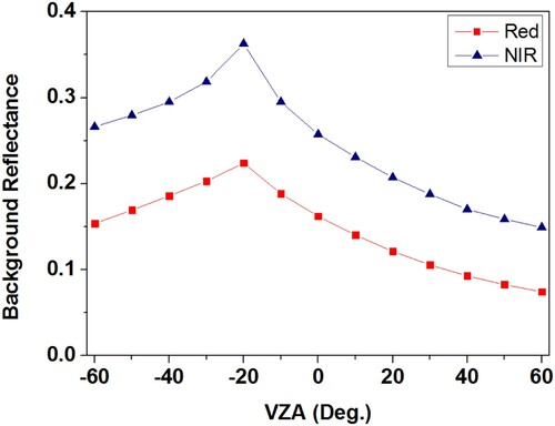
Considering the actual canopies in RAMI are either mixed forests or with relatively high variance in crown structures, which hardly serve as the input parameters in GOST2 and GOST, only two abstract RAMI-IV stands: HET-10 and HET-20 were selected in this study. Tree crowns are sphere-shaped with leaves randomly distributed in each crown. The structural and optical parameters of stands in the two RAMI stands are identical. For example, tree size, LAI of individual sphere, leaf reflectance, and background reflectance are all the same between the two stands (Table 1). The only difference between the two stands is the tree number: 2574 trees in the HET-10 and 5093 trees in the HET-20. The background BRF pattern in the two RAMI stands is non-Lambertian. Both backgrounds are bare soil in two RAMI stands. The BRFs of the anisotropically scattering background are expressed with the parametric RPV model and are shown in Figure 1. The tree positions in the two RAMI stands can be downloaded on the website. For additional information, please refer to (Widlowski et al. 2013) and the RAMI-IV website: https://rami-benchmark.jrc.ec.europa.eu/HTML/RAMI-IV/RAMI-IV.php.

Figure 1. The background reflectance in the two RAMI stands.

3. Canopy reflectance model

3.1. GOST2

GOST2 is an upgrade version of GOST (Fan, Li, and Liu 2015) which is developed based on the Four-Scale model, and can be used to simulate canopy BRF for forests on sloping terrain. The sunlit and shaded foliage in the view direction can be easily separated using a ray-tracing procedure in GOST. However, because GOST has high computational demands, the model was updated to GOST2 to improve computational efficiency. GOST2 has been validated in natural forests (Chen and Leblanc 1997; Leblanc et al. 1999), while its performance in forest plantations is unknown so far. Here, we use GOST2 as a comparison with GOFP.

GOST2 simulates natural forests CR considering the canopy architecture at four scales: tree groups, tree crown geometry, branches, and foliage elements. With consideration of the patchiness among trees in natural forests, the Poisson model and the Neyman model are used to describe the tree distribution in a forest stand. In the Poisson model, trees are assumed to be distributed randomly in the forest stands. In the Neyman model, trees are assumed to be distributed in each cluster or group randomly; the centers of clusters or groups are also assumed to be distributed in the forest stand randomly; the number of tree crowns in each group or cluster is random. Compared with the Poisson model, in which trees are assumed to be randomly distributed within the forest stand, the Neyman model enhances the randomness and patchiness among the trees in the stand. Therefore, it is also known as the double-Poisson model.

GOST2 is based on the assumption that: the spectral reflectance of forest canopies is composed of four scene components: sunlit foliage (P_T,), sunlit ground (P_G), shaded foliage (Z_T), and shaded ground (Z_G). Each proportion is multiplied by its reflectivity factor that depends on the wavelength used. Then, the canopy reflectance can be calculated as follows (Chen and Leblanc 1997; Fan, Li, and Liu 2015): (1) $R=R_T\ast P_T+R_G\ast P_G+R_{ZT}\ast Z_T+R_{ZG}\ast Z_G$(1) where R_T, R_G, R_ZT, and R_ZG are the reflectivity factors of the P_T, P_G, Z_T, and Z_G in GOST2, respectively. The structure of canopies, such as the distribution and size of the tree crowns, are expressed mathematically and the areas of the four scene components (P_T, P_G, Z_T, and Z_G) can be calculated, respectively. R_T and R_G are input parameters. A p theory of collision probability is added in GOST2 to calculate R_ZT and R_ZG (Omari, White, and Staenz 2009; Fan, Li, and Liu 2015).

The input parameters in GOST2 include three main types: (1) structural parameters: tree density, crown size, LAI, and clumping index; (2) optical parameters: the reflectance and transmittance of the leaf and the reflectance of background; and (3) observation and sun angles: view zenith angle (VZA), sun zenith angle (SZA), and relative azimuth angle between view and sun (RAA). The output is the CR including canopy BRF. Both GOST and GOST2 have been compared with many other CR models and validated using the multi-angular satellite images. For additional information about GOST2, please refer to (Fan et al. 2014a, 2014b, 2015).

3.2. GOFP

GOFP, which is based on the Four-Scale model and GOST2, is specifically designed for simulating the CR of forest plantations (Geng et al. 2017).

The main difference of GOFP from Four-Scale and GOST2 is that the former two emphasise the patchiness and randomness effects among trees in a forest stand and use the Neyman and the Poisson model to describe the tree distribution. However, GOFP emphasises the exclusion effect among trees in a forest stand and uses a hypergeometric model rather than the Neyman or the Poisson model to describe the spatial relationship among trees, based on the fact that each tree crown can occupy its own space (such as the crown above ground and root below ground occupy a ‘private’ space or ‘crust’ which can hardly be occupied or overlapped by other trees, Figure 2(c)). The hypergeometric model describes the probability of k successes in n draws, without replacement, from a finite population of size N that contains exactly m successes. Its probability mass function is given by: (2) $f(k,n,m,N)=\left(\begin{array}{c}m\\ k\end{array}\right)\left(\begin{array}{c}N-m\\ n-k\end{array}\right)/\left(\begin{array}{c}N\\ n\end{array}\right)$(2)

Figure 2. Schematic of three tree spatial patterns that lead to different forest coverages. (Green circles mean crowns at nadir. (a) the Poisson model, only randomness among trees are considered which produces a medium degree of overlap among trees; (b) the Neyman model, both patchiness and randomness among trees are considered which produces the most overlap among trees and the minimum vegetation coverage; and (c) the hypergeometric model, both exclusion effect and randomness among trees are considered which produces a minimum degree of overlap among trees and the maximum forest coverage in all three models).

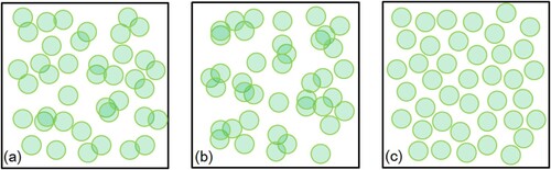
If n = 1, the hypergeometric distribution is the binomial distribution which is an independent event; if n > 1, it is a conditional probability because every foregoing sampling result could affect the subsequent sampling probability. The essential difference between the Poisson model and the hypergeometric model is that the former uses random sampling with replacement, while the latter uses random sampling without replacement. This characteristic of the hypergeometric model can be used to describe the tree distribution in the forest plantation stands: (1) the characteristic of ‘random sampling’ in the hypergeometric model can be used to express the randomness of the tree distribution in the forest stands; (2) the characteristic of ‘without replacement’ in the model can be used to describe the exclusion effect among trees in the stands. Compared with the Poisson random model and the Neyman model, both the randomness and exclusion effect among trees can be considered in the hypergeometric model. The different descriptions of three distributions with the tree models are shown in Figure 2. The hypergeometric model has an exclusion effect among trees, leading to a minimum degree of overlap among the trees at nadir and the maximum forest coverage in all three forest stands in Figure 2.

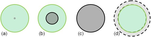
The framework and computational process of the two GO models are similar. For example, the background was divided into sunlit and shaded parts using a phase function; the leaves are divided into sunlit and shaded parts using a ray-trace method; and the multiple scattering was calculated using the p theory (Fan et al. 2014a, 2014b; Fan, Li, and Liu 2015). The input parameters are similar to GOST2. In addition, it requires a very important distance parameter RASD (relative allowable shortest distance between centers of two adjacent crowns divided by the mean diameter of the crown). It controls the spatial pattern of the tree crowns in the forest stand and is used to quantitatively describe the exclusion effect among trees and calculate the canopy gap fraction at various VZAs in the forest plantations (Geng et al. 2016). When RASD = 0, it means that there is no exclusion effect among trees. Trees are randomly distributed in the forest stand and the hypergeometric model is actually the Poisson model. In other words, the Poisson model is a special case of hypergeometric model for describing tree distributions, and it can be completely replaced by hypergeometric model (Geng et al. 2017). The larger value of RASD means a stronger exclusion effect among trees in the forest stand. When RASD > 1, it means that the nearest distance between trees is larger than the crown diameter and any two crowns in the stands are separated at nadir (Figure 1(c)). The default value of RASD in GOFP is equal to 1, indicating that the ‘private’ space for each crown is the crown itself and the nearest two crowns are allowed to be tangent but not allowed to intersect with each other at nadir.

In summary, compared with GOST2, GOFP considers both the randomness and repulsion effect among trees (Figure 3). For additional information about the hypergeometric model, please refer to Geng et al. (2016); and for additional information about GOFP, please refer to Geng et al. (2017).

Figure 3. Schematic of the hypergeometric model for tree crowns in a forest plantation stand with an increment of RASD. (Green circles represent crowns at nadir; gray circles are the ‘crust’ of trees, which is a rigid body and cannot overlap with other crowns. The size of the gray circles represents the exclusion distances among tree crowns. (a) the size of the ‘crust’ is zero, RASD = 0, the hypergeometric model is actually the Poisson model; (b) the ‘crust’is inside the crown, RASD < 1; (c): ‘crust’ is the crown itself, RASD = 1; and (d) the ‘crust’ is larger than the crown, RASD > 1. The oblique outside of the crown is the pseudo reject area and need to be removed when calculating the gap fraction because the region is not actually a crown)).

4. Results

4.1. Tree distribution

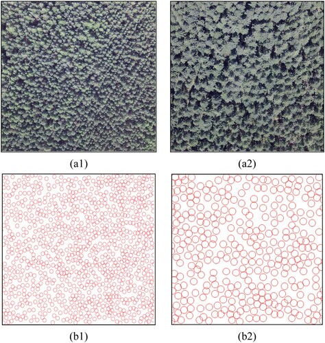
Forest plantations are planted in such a way that each tree can occupy a ‘private’ space to obtain enough sunlight, water, and nutrients. Tree crowns in forest plantations barely overlap with each other from the nadir view. Tree positions were provided on the RAMI website, and are shown in Figure 4. Crowns can be discerned clearly from high-resolution images obtained from a UAV platform at nadir (Figure 5(a)). Each tree crown is identified and shown in Figure 5(b) from the high-resolution images. Rare overlaps among trees can be found in both Saihanba forest plantation stands.

Figure 4. Tree positions in the two RAMI forest stands ((a) HET-10; (b) HET-20. Red circles are tree crowns at nadir).

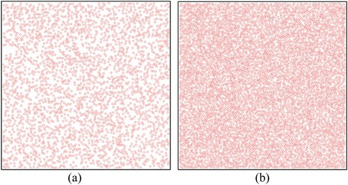
Figure 5. Tree positions in sample plots of two forest plantations (1: PS stand; 2: DL stand). ((a) Exclusion distances among trees are found in the plot from UAV high-resolution images. (b) Tree positions in the sample plot are identified from UAV high-resolution images. The red circles represent crowns at nadir).

To quantitatively describe the tree distribution, the two RAMI forest stands (about 100 × 100 m) in Figure 4 and the two Saihanba forest stands (about 130 × 130 m) in Figure 5 were equally divided into 100 quadrats. The numbers of quadrats with a certain number (i) of trees were counted and the probability density distribution of finding i trees in a quadrat was plotted in Figure 6. The Neyman model with m₂ = 2, the Poisson model and the hypergeometric model with RASD = 1 were compared with the measurement. Here, m₂ in the Neyman model is the mean number of trees in a cluster. In the Four-Scale model, the default value of m₂ is equal to 5. The larger value of m₂ means more strong patchiness effect among trees (Chen and Leblanc 1997).

Figure 6. The tree distribution in the four forest stands divided in 100 quadrats compared with the Poisson, Neyman and hypergeometric model (m₂ in the Neyman model indicates the average number of trees in a cluster. The default value of m₂ in the Four-Scale model is 5. A larger value of m₂ means stronger clumping of the trees and a broader line distribution (Chen and Leblanc 1997)).

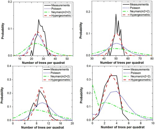
As shown in Figure 6, the lines of measurements are distributed narrowly around the mean number of trees per quadrat (about 25 trees for the HET-10 stand, 50 trees for the HET-20 stand, 9 trees for the PS stand, and 3 trees for the DL stand) in the four forest plantation stands; while the lines of the Poisson and the Neyman distributions are much broader, indicating that the probability of finding i trees in a quadrat exhibit strong randomness. Measurements from the sample plot show an obvious discrepancy of the tree distribution from the Poisson and the Neyman random cases. Both the height and width of the hypergeometric model lines show good consistency with the measurement. Especially for the two Saihanba stands, the lines between the hypergeometric model and the measurement are nearly coincident in Figure 6, indicating that the probability of finding i trees in a quadrat is a relatively stable value.

In summary, according to the figures of the probability density distributions, trees in the four forest stands described by the hypergeometric model match the measurement better than the Neyman model and the Poisson model. The imperfect tree distribution in the forest plantation described in GOST2 certainly affects CRs. The next section will present the influence.

4.2. Canopy reflectance (CR)

4.2.1. Comparison of CR in the two RAMI stands

Gap fraction (GF) is the main difference between GOFP with the hypergeometric model and GOST2 with the Poisson model. Therefore, it is necessary to compare GF before comparing BRF. The calculations of GF were shown in Geng et al. (2017).

For validating GF in GOFP, we used the image classification method to calculate the GF of two RAMI stands. Only diffuse light was used in the two forest stands in the 3D MAX software, and a camera was set at 0–80° on the two stands. Thus, there was no shadow in the view direction and the scene images can be easily classified into background and crown, and the GF could be calculated directly from classified images (Figure 7). The comparison of the GF in the two RAMI forest stands are shown in Figure 8: suffixes ‘_c’ is the GF used the image classification method; ‘_p’ is the GF in GOST2 with the Poisson distribution; ‘_h’ is the GF in GOFP with the hypergeometric distribution. For the detailed calculation of the GF in GOFP and GOST2, please refer to Geng et al. (2016, 2017).

Figure 7. Image classification methods for calculating GF at different VZAs in the HET-20 stand (Green areas are crowns; red areas are backgrounds).

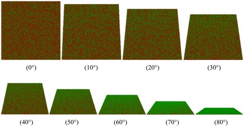
Figure 8. Comparison of gap fractions with the tree Poisson distribution and hypergeometric distribution.

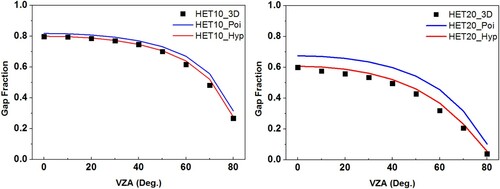
From Figure 8, the GFs calculated with the hypergeometric model are highly consistent with those of image classification indicating that GOFP performed well in calculating the GFs at various VZAs for forest plantation. The GFs in GOST2 with the Poisson distribution are generally larger than those in GOFP. It means that more crowns or less background can be seen in GOFP than those in GOST2 at various VZAs.

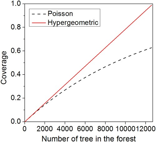
The difference in GF between GOFP and GOST2 is obviously larger in the HET-10 than that in the HET-20. It is because that the crown density and vegetation coverage in the HET-10 is only a half of those in the HET-20 (Table 1). According to previous studies, the difference between GOFP and GOST2 is closely related with the tree density and forest coverage (Geng et al. 2017). Figure 9 is a comparison of forest coverage between the Poisson model and the hypergeometric model with RASD = 1. The crown radius is 0.5 m. From Figure 9, with the increment of tree density or number, the differences of forest coverage between the two models increase obviously. The difference could be ignored in very sparse forest stands, where few leaves can be seen no matter what the tree distribution is.

Figure 9. Comparison of vegetation coverage varying with tree number between the Poisson model and the hypergeometric model with RASD = 1 (crown radius is 0.5 m).

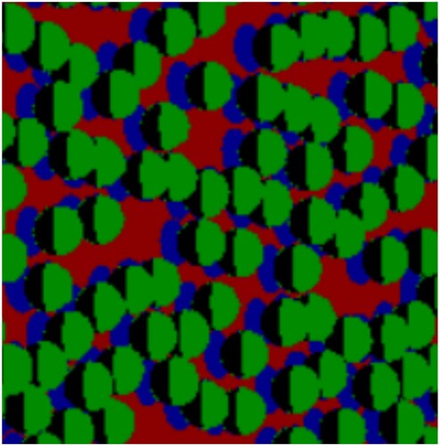
The differences of GF between the two GO models inevitably lead to the differences of the four scene components area ratios. Taking the HET-20 stand for example, the whole scene was divided into the four components (sunlit background, shaded background, sunlit leaves, and shaded leaves) using the image classification method in 3D MAX software. The comparisons of the classified and simulated area ratios of the four scene components in the principal plane from GOST2 with the Poisson tree distribution and GOFP with the hypergeometric tree distribution are shown in Figure 10.

Figure 10. Comparison of the classified and simulated area ratios of the four scene components in the principal plane from GOST2 with the Poisson tree distribution and GOFP with the hypergeometric tree distribution.

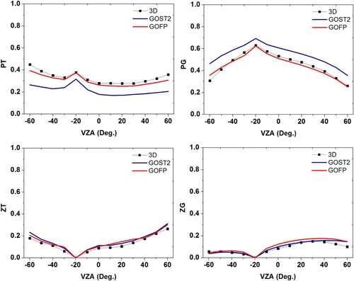
The four-component area ratios showed the hotspot effect at VZA = 20°. The two sunlit parts (leaves and background) showed peaks around VZA = 20°. The four-component area ratios simulated with GOFP show a better consistency with the classification results in 3D MAX than GOST2. The differences in the two sunlit parts (leaves and background) between GOFP and GOST2 are similar to the differences of GFs between two models: the sunlit leaves area ratios in GOFP are obviously larger than those in GOST2; on the contrary, the sunlit background area ratios in GOFP are obviously larger than those in GOST2. It worth noting that the differences in the shaded leaves area ratios between the two models are smaller than those in the sunlit leaves area ratios. It is because that the shaded leaves often locate the low part of crown (sun zenith angle is 20°) and the tops of the crown are more likely to be illuminated and visible than the lower portions, which are more likely to be overlapped by neighboring crowns in the view directions (Figure 11).

Figure 11. Schematic of the area ratios of the four scene components at VZA = 60° in the forward direction (Green regions are sunlit crowns, black regions are shaded crowns, red regions are sunlit background, and blue regions are shaded background. Black regions are highly overlapped with each other, while green regions are rarely overlapped by neighboring crowns in the view directions).

Up to now, there are more than eighty BRF models have been tested in the RAMI platform. For the two chosen RAMI stands, there are eleven bidirectional reflectance distribution function (BRDF) models’ BRFs being compared together. The RAMI does not provide the numerical values of these models’ results but only show the pictures on the website. For convenience, only two models were chosen here, that is, discrete anisotropic radiative transfer (DART) and invertible forest reflectance model (INFORM). DART is a 3-D radiation interaction model, and has been widely used in simulating BRDF, remote sensing images, and the spectral radiation budget of many 3D natural objects (e.g. trees, grass and soil) from the ultraviolet to the thermal infrared bands (GastelluEtchegorry et al. 1996; Gastellu-Etchegorry, Martin, and Gascon 2004). INFORM is a hybrid model that integrates the Forest Light Interaction Model (FLIM) (Rosema et al. 1992), Scattering by Arbitrary Inclined Leaves (SAILH) (Verhoef 1985), and PROSPECT (Jacquemoud and Baret 1990) to simulate the BRF of forest canopies. It is worth noting that tree distributions in INFORM are similar to GOST2 because trees are assumed randomly distributed in a stand in FLIM. Both DART and INFORM are widely used in the BRF modeling and parameter retrieval during the past two decades (Yuan et al. 2015; Darvishzadeh et al. 2019; Wu et al. 2019; Wang et al., 2020a). In the RAMI website, there are obvious differences between INFORM and other BRDF models in most cases. It is an important reason that we chose INFORM here. For more information about the all BRDF models’ simulations, please see the RAMI website: https://rami-benchmark.jrc.ec.europa.eu/HTML/RAMI-IV/RESULTS/ABSTRACT_CANOPIES/HETEROGENEOUS/ANISOTROPIC_BACKGROUND/BRF_in_principal_plane_(total)/BRF_in_principal_plane_(total).php.

The BRF simulations of DART and INFORM were digitalized from figures in the above RAMI website and shown in Figure 12 to compare with GOFP and GOST2 results. In the red band (Figure 12 left), there is no obvious difference in the BRFs among the four models in the HET-10 stand, although the BRFs of GOST2 are slightly larger than those in the other three BRDF models for this stand. While the BRFs of GOST2 are obviously larger than simulations of the other three models in the HET-20 stand. It is because that the GF is overestimated at each VZA for the Poisson model. BRFs simulated by the GOST2 were closer to INFORM than GOFP and DART. This is because the trees are assumed to randomly distribute in both INFORM and GOST2. As the background reflectance is significantly larger than leaf reflectance in red bands for both RAMI stands (Figure 1). BRFs in GOST2 and INFORM with the Poisson model are overestimated. After the correction for the tree distributions in the two RAMI stands, the BRFs of GOFP are highly consistent with the simulations of DART, indicating the correction for the tree distribution in the two RAMI stands is necessary.

Figure 12. Comparison of BRFs using the four BRDF models in the principal plane in the red and NIR bands, respectively.

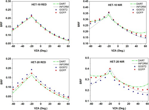
In the NIR band (Figure 12, right), the BRFs simulated with GOFP and GOST2 show good consistence with those simulated with DART and INFORM at low VZAs in the HET-10 stand, while the BRFs simulated with GOST2 and INFORM are lower than the simulations of GOFP and DART in the HET-20 stand. It is because that the leaf reflectance is larger than the background reflectance in the NIR band in the two RAMI stands (Figure 1). The BRF shapes in NIR band in GOST2 are similar to those in INFORM, but deviate from DART simulations, especially at larger VZAs. After correction for the tree distribution, the BRF simulations in GOFP are closer to DART simulations than GOST2 and INFORM at most VZAs.

In summary, from the GF, four component area ratios, and BRF simulation, GOFP using the hypergeometric model to describe the tree distribution shows better performance than GOST2 using the Poisson model. The BRFs of GOST2 are overestimated in the red band, but underestimated in the NIR band. The BRFs of GOFP are closer to the results of DART than GOST2.

4.2.2. Comparison and validation of CR in the two Saihanba stands

The CR measured by the remote sensor mounted on the UAV platform in the principal plane in the two Saihanba forest stands is shown in Figure 13. The measurements of canopy BRFs from the UAV platform exhibit strongly ‘bowl-shaped’ in the two Saihanba forest stands. They are typical forest canopy BRF characteristic and show high quality. Specifically, (1) the hotspot effect is captured well, especially for the PS and DL stands: the maximum value of CR exists at the hotspot in both the red and NIR bands; (2) the values of CR in the backward direction are higher than those in the forward direction. The CRs at the dark-spot (about 20° in the backward direction) are obviously lower than those at other VZAs, indicating that the dark-spot effect is captured well in both PS and DL stands.

Figure 13. Comparison of BRFs measured by UAV and simulated by the four BRDF models in the principal plane in the 670 nm (red) and 800 nm (NIR) bands, respectively.

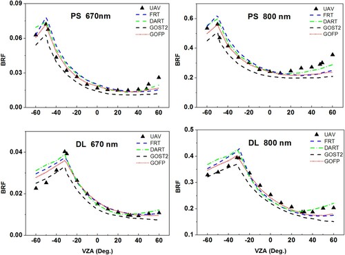
Here, we used two BRDF models as comparisons with the simulations of GOFP and GOST2. DART was also used here. The forest radiative transfer model (FRT) developed to simulate both the upward and downward radiances in a forest stand at Tartu Observatory, Estonia (Kuusk and Nilson 2000). It has been validated in several mixed forests (Kuusk et al. 2008; Kuusk, Kuusk, and Lang 2009) and widely applied in simulating BRFs for forest canopies (Kuusk et al. 2010; Kuusk, Kuusk, and Lang 2014a, 2014b; Widlowski et al. 2015). An important reason for choosing FRT here is a key parameter describing tree distribution deviating from the Poisson model. Fisher’s grouping index (GI), which means the relative variance of the number of trees in the area, was used to describe the tree distribution in a stand in FRT (Nilson 1999; Kuusk and Nilson 2000). The tree distribution parameters for the Saihanba forest stands are about 1.6 in FRT, indicating there is nearly no overlap among tree crowns at nadir. This is suitable for the two Saihanba stands. Specific tree positions serve as input parameters in DART. The other input parameters of four BRDF models are listed in Tables 1 and 2. The tree distribution is the hypergeometric model with RASD = 1 in GOFP, while trees are assumed to meet the Neyman model with m₂ (average number of trees in a cluster) = 2 in GOST2.

Table 2. The observation angles and sun angles in the four forest stands.

Parameter	HET10 & HET20	PS	DL
Date	–	21.08.2019	21.08.2019
Time, GMT	–	7:20–7:40	3:10–3:30
Sun zenith angle (SZA, Deg.)	20	52	33
Sun azimuth angle (SAA, Deg.)	0	250	160
View zenith angle^a (VZA, Deg.)	−60–60	−60–60	−60–60
View azimuth angle (VAA, Deg.)	0	−105, 75	165, −15
Relative azimuth angle (RAA, Deg.)	0	355, 185	5, 175

The BRF simulations of the four BRDF models are shown in Figure 13. All four models’ simulations generally show a relatively good consistency with the measurement in two aspects: the magnitude and width of the hotspot. The magnitude of the hotspot is mainly influenced by geographical information of the observation and sun. While, compared with GOST2, the BRFs simulated by GOFP shows a higher consistency with the measurement at most VZAs in the two forest stands. Corresponding to the results shown in Section 4.1, the Neyman model increases the patchiness and clumping effect among trees, decreasing the forest coverage and increasing the background area or ratio observed by the remote sensor. A larger amount of background that can be seen in GOST2, meanwhile, the background reflectance is much lower than the leaf reflectance in the red band in the two Saihanba forest stands (Table 1). As a result, the BRFs simulated by GOST2 are underestimated at most VZAs in the two Saihanba forest stands in Figure 13 (left). Similarly, the leaf reflectance is also larger than background reflectance in the NIR band (Table 1). Therefore, the simulations of GOST2 are also underestimated in the NIR band at most VZAs in the two Saihanba forest stands. The difference in BRF between GOST2 and GOFP is closely related to VZAs: the difference is more obvious at low VZAs (such as at nadir) than that at large VZAs. It is because that the differences in forest coverage in the view direction between the two tree distribution models are more marked at low VZAs than those at large VZAs.

Similar to the BRF simulations in the two RAMI stands, the BRFs simulated with GOFP and GOST2 are underestimated at large VZAs in the forward direction, especially in the NIR band. DART shows a good performance in the forward direction and at the hotspot with respect to the two GO models. The BRF simulations in GOST2 are the lowest among the four BRDF models’ simulations. After correction for the tree distribution in GOFP, the BRF simulations are closer to those in DART and FRT than those in GOST2.

Nearly all BRF simulations in the forward direction are lower than the measured BRFs. The underestimation for all the models may be due to two reasons: first, the measured BRFs which were closely related to the sunlight. In practice, BRFs at all zenith angles in a stand were observed in a whole flight: canopy reflectance in the backward directions was firstly observed, and then was observed at nadir; finally, canopy reflectance in the forward directions was observed. A whole flight needed about 20 min. Therefore, there was the slightly change in sunlight. It may lead to the overestimation of measured BRFs in the forward directions. Another reason may be that the abstract of parameters in the BRDF models in this study is not particularly correct. For example, the sizes of all crowns in a stand are identical in all models (including DART). It is common problem for nearly all GO models.

In summary, GOFP is compared well with GOST2 in the two RAMI forest stands and validated in the two Saihanba forest stands at most VZAs. GOFP shows a better consistency with the simulations of DART and the measurements in the two Saihanba forest stands than GOST2 in most cases because the tree distribution in forest plantations is described more reasonably in GOFP. The GF simulated by GOST2 is generally overestimated, which caused some difference in BRFs from other BRDF models. The performances of two GO models are good for relatively sparse forest stands, while GOFP is recommended for simulating CR for forest plantations, especially for dense forest plantation stands.

5. Discussion

Forest plantations are planted by human, and trees in forest plantations at the stand level hardly completely overlap each other at nadir to ensure each trees can occupy a private space to acquire enough light, water, and nutrients. Comparing with natural forests, the particular distribution in the forest plantations lead to the largest degree of forest cover and lowest degree of soil area exposed to the wind and sunlight. Therefore, they play a very key role in fixing the sandy soil and reducing desertification.

5.1. The hypergeometric model

Tree distributions are always composed of randomness and regularity. The hypergeometric model considers both randomness and repulsion effects among tree crowns. The essence of presenting the hypergeometric model is not to describe the tree distribution absolutely accurately, but to describe the tree distribution with more accurate than the Poisson model and the Neman model in the forest plantation stand. In fact, there still some difference in tree distribution between the hypergeometric model and the measurements (Figure 6). There are many complex models (such as the spatial point pattern analysis) in the field of community ecology describing the tree distribution more accurately. While these complex models cannot be directly used in GO models because of the following two reasons:

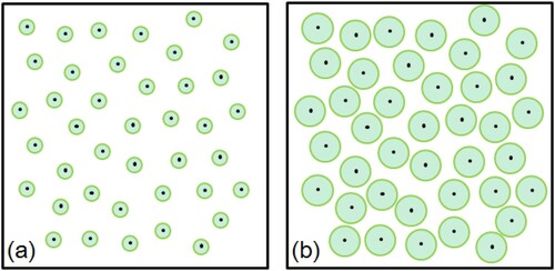
1. The crown sizes need to be considered. The spatial point pattern analysis, such as the Neyman-A type model, was often used to describe the tree distribution in a stand in the field of community ecology. This method deems each tree crown as a point. The number of points (tree crowns) is counted in each quadrat, and the statistic parameters (such as variance) are used to quantify the tree spatial agglomeration distribution. While, the spatial point pattern analysis method may not be used in the BRDF model directly, because the exclusion distance among trees and trees size also need to be considered. Figure 14 shows two stands with the same tree positions. The stand (a) can be deemed as a young stage canopy and the stand (b) can be deemed as middle-aged. The numbers of tree crown in each quadrat are identical because the centers of tree positions in the two stands are identical to each other. While the tree distributions in two stands cannot be deemed as the same one as mentioned in Section 3. Trees are distributed regularly and meet the hypergeometric model in both stands. While, the RASD in the two stands are significantly different from that in the stand (b), the RASD is about one due to that the nearest distance among trees in the stand is about the crown diameter; while the RASD in the stand (a) is obviously larger than 1. Both the distance among tree centers and crown sizes are considered in the hypergeometric model, while only distance among trees centers are considered in the spatial point pattern analysis. This is the main difference between the two methods.

2. Many models for describing the tree distribution are too complicated to easily calculate the GF, which is a very important intermediate parameter in nearly all GO models. The Poisson model and the binomial distribution were often used in GO models because its convenience and effectiveness in calculating the overlapping area among tree crowns at various VZAs. Complex models, such as the Gibbs model and hybrid Gibbs model (Perry, Miller, and Enright 2006; Gray and He 2009; Wang et al., 2020b), have the abilities to describe the tree distribution more accurately; while they have difficulty calculating the overlapping area among tree crowns at various VZAs. Therefore, these models need to be modified before adding into GO models for describing the tree distribution and simulating the canopy BRF.

Figure 14. Schematic of two stands with the same tree positions but the different tree distributions in this study. (Green circles represent crowns at nadir, black dots mean trunks; RASD is greatly larger than 1 in stand (a), but is about 1 in stand (b)).

The hypergeometric model in GOFP with a simple distance parameter RASD is actually an improved model with respect to the Poisson model. The Poisson model can be completely replaced by the hypergeometric model when RASD = 0. This operation can keep the high efficiency and improve the accuracy of the GO model. The hypergeometric model in this study may be a uniform module that can be used in many other forest-canopy GO models because that the description of the tree distribution is a necessary step for near all forest-canopy GO models.

5.2. Spatial scale effect

The tree distribution is closely related to spatial scale. In this study, trees in two representative forest plantation stand exhibited clear exclusion effects and met the hypergeometric model better than the Neyman model or the Poisson model in a stand scale. Nevertheless, patchiness exists in many forest plantation stands in a larger scale than a stand. The hypergeometric model focuses on the repulsion among trees, while patchiness and clumping among trees are not considered in GOFP. GOFP should not be used for simulating the CR at a large scale where clear patchiness effects in the study area. The Neyman model may be more suitable for describing the tree distribution than the hypergeometric model. One important hypothesis in the Neyman model is that trees are exclusive or regularly rather than randomly distributed in each cluster. This is not exactly correct because in some cases trees show exclusion or regular effects rather than randomness in each cluster even though trees show patchiness in the whole image. This is actually the spatial scaling effect, which have been studied by many researchers (Zeng et al. 2020; Gong et al. 2013). Thereafter, the whole images can be divided into several patches or clusters. Firstly, trees can be assumed to meet the hypergeometric model in each cluster. Secondly, the clusters can be assumed to meet the hypergeometric model. Similarly, the CR in each cluster can be simulated by GOFP. Finally, the CR in the whole image may be obtained by averaging the CR in each cluster.

It is impossible to use a uniform model to accurately describe tree distribution at any scale and in any situation. If the trees are distributed irregularly or the existing mathematical models hardly describe the tree distribution, 3D models, such as DART, RAPID (Huang, Qin, and Liu 2013), and RGM (Xie et al. 2012), are suggested to use to simulate the canopy BRF.

6. Conclusions

Forest plantation is an important type of forest with different tree distribution pattern from natural forest. GOFP is a relatively new CR model for forest plantations, using a flexible hypergeometric model instead of the Poisson model to describe tree distribution in a forest stand. It has been validated using the MODIS images with coarse resolution.

In this study, GOFP was validated in two forest plantation stands in the largest forest plantation in the world, Saihanba Forestry Center, using an in situ dataset of structure and optical measurements on a UAV platform. Meanwhile, the results of GOFP were compared in two RAMI stands. The results showed that: (1) the hypergeometric model in GOFP for describing the tree distribution in forest stands performs well in all four stands. (2) CR simulated from GOFP showed a good consistency with the simulations of DART in two RAMI stands, and the measurements from UAV in the two Saihanba forest stands. The results validated the reliability of GOFP in describing tree distribution and in simulating CR for forest plantations. Both of random and exclusion effect among trees should be considered for describing tree distribution in forest plantation. Future directions will focus on the other particular tree distribution, that is, grid-shape and line-shape distribution to validate and refine GOFP for its applications to different kinds of forest stands.

Acknowledgments

The authors thank the two anonymous reviewers for their constructive comments and advices.

Disclosure statement

No potential conflict of interest was reported by the author(s).

Additional information

Funding

This research was funded by the National Natural Science Foundation of China (grant no. 41701383, 42071392, and 41801234), Anhui Provincial Natural Science Foundation (grant no. 1808085QD105), the Fundamental Research Funds for the Central Universities of China (grant no. PA2020GDSK0083), and the Fund of Key Laboratory of Information Perception and Systems forPublic Security of MIIT (Nanjing University of Science and Technology) (grant no. 202003).

Notes

^a LR: leaf reflectance; TR: leaf transmittance; BR:background reflectance.

^a Negetive values mean VZA in the backward direction; positive values mean VZA in the forward direction.

References

- Chen, J. M., and S. G. Leblanc. 1997. “A Four-scale Bidirectional Reflectance Model Based on Canopy Architecture.” IEEE Transactions on Geoscience and Remote Sensing 35 (5): 1316–1337.
- Chen, J. M., C. H. Menges, and S. G. Leblanc. 2005. “Global Mapping of Foliage Clumping Index Using Multi-angular Satellite Data.” Remote Sensing of Environment 97 (4): 447–457.
- Chopping, M., L. Su, A. Rango, J. Martonchik, D. Peters, and A. Laliberte. 2008. “Remote Sensing of Woody Shrub Cover in Desert Grasslands Using MISR with a Geometric-Optical Canopy Reflectance Model.” Remote Sensing of Environment 112 (1): 19–34.
- Darvishzadeh, R., A. Skidmore, H. Abdullah, E. Cherenet, A. Ali, T. Wang, W. Nieuwenhuis, et al. 2019. “Mapping Leaf Chlorophyll Content from Sentinel-2 and RapidEye Data in Spruce Stands Using the Invertible Forest Reflectance Model.” International Journal of Applied Earth Observation and Geoinformation 79: 58–70.
- Deng, F. 2006. “Algorithm for Global Leaf Area Index Retrieval Using Satellite Imagery.” IEEE Transactions on Geoscience and Remote Sensing 44 (8): 2219–2229.
- Fan, W., J. M. Chen, W. Ju, and N. Nesbitt. 2014a. “Hybrid Geometric Optical-radiative Transfer Model Suitable for Forests on Slopes.” IEEE Transactions on Geoscience and Remote Sensing 52 (9): 5579–5586.
- Fan, W., J. M. Chen, W. Ju, and G. Zhu. 2014b. “GOST: A Geometric-optical Model for Sloping Terrains.” IEEE Transactions on Geoscience and Remote Sensing 52 (9): 5469–5482.
- Fan, W., J. Li, and Q. Liu. 2015. “GOST2: The Improvement of the Canopy Reflectance Model GOST in Separating the Sunlit and Shaded Leaves.” IEEE Journal of Selected Topics in Applied Earth Observations and Remote Sensing 8 (4): 1423–1431.
- Gastellu-Etchegorry, J. P., E. Martin, and F. Gascon. 2004. “DART: A 3D Model for Simulating Satellite Images and Studying Surface Radiation Budget.” International Journal of Remote Sensing 25 (1): 73–96.
- GastelluEtchegorry, J. P., V. Demarez, V. Pinel, and F. Zagolski. 1996. “Modeling Radiative Transfer in Heterogeneous 3-D Vegetation Canopies.” Remote Sensing of Environment 58 (2): 131–156.
- Geng, J., J. M. Chen, W. Fan, L. Tu, Q. Tian, R. Yang, Y. Yang, L. Wang, C. Lv, and S. Wu. 2017. “GOFP: A Geometric-optical Model for Forest Plantations.” IEEE Transactions on Geoscience and Remote Sensing 55 (9): 5230–5241.
- Geng, J., J. Chen, L. Tu, Q. Tian, L. Wang, R. Yang, Y. Yang, et al. 2016. “Influence of the Exclusion Distance Among Trees on Gap Fraction and Foliage Clumping Index of Forest Plantations.” Trees 30 (5): 1683–1693.
- Gong, P., J. Wang, L. Yu, Y. Zhao, Y. Zhao, L. Liang, Z. Niu, et al. 2013. “Finer Resolution Observation and Monitoring of Global Land Cover: First Mapping Results with Landsat TM and ETM+ Data.” International Journal of Remote Sensing 34 (7): 2607–2654.
- Gray, L., and F. He. 2009. “Spatial Point-pattern Analysis for Detecting Density-dependent Competition in a Boreal Chronosequence of Alberta.” Forest Ecology and Management 259 (1): 98–106.
- He, L., J. Liu, J. M. Chen, H. Croft, R. Wang, M. Sprintsin, T. Zheng, et al. 2016. “Inter- and Intra-annual Variations of Clumping Index Derived from the MODIS BRDF Product.” International Journal of Applied Earth Observation and Geoinformation 44: 53–60.
- Huang, H., W. Qin, and Q. Liu. 2013. “RAPID: A Radiosity Applicable to Porous Individual Objects for Directional Reflectance Over Complex Vegetated Scenes.” Remote Sensing of Environment 132: 221–237.
- Jacquemoud, S., and F. Baret. 1990. “PROSPECT: A Model of Leaf Optical Properties Spectra.” Remote Sensing of Environment 34 (2): 75–91.
- Kuusk, A., J. Kuusk, and M. Lang. 2009. “A Dataset for the Validation of Reflectance Models.” Remote Sensing of Environment 113 (5): 889–892.
- Kuusk, A., J. Kuusk, and M. Lang. 2014a. “Modeling Directional Forest Reflectance with the Hybrid Type Forest Reflectance Model FRT.” Remote Sensing of Environment 149: 196–204.
- Kuusk, A., J. Kuusk, and M. Lang. 2014b. “Measured Spectral Bidirectional Reflection Properties of Three Mature Hemiboreal Forests.” Agricultural and Forest Meteorology 185: 14–19.
- Kuusk, A., and T. Nilson. 2000. “A Directional Multispectral Forest Reflectance Model.” Remote Sensing of Environment 72 (2): 244–252.
- Kuusk, A., T. Nilson, J. Kuusk, and M. Lang. 2010. “Reflectance Spectra of RAMI Forest Stands in Estonia: Simulations and Measurements.” Remote Sensing of Environment 114 (12): 2962–2969.
- Kuusk, A., T. Nilson, M. Paas, M. Lang, and J. Kuusk. 2008. “Validation of the Forest Radiative Transfer Model FRT.” Remote Sensing of Environment 112 (1): 51–58.
- Leblanc, S. G., P. Bicheron, J. M. Chen, M. Leroy, and J. Cihlar. 1999. “Investigation of Directional Reflectance in Boreal Forests with an Improved Four-Scale Model and Airborne POLDER Data.” IEEE Transactions on Geoscience and Remote Sensing 37 (3): 1396–1414.
- Li, X., and A. H. Strahler. 1985. “Geometric-optical Modeling of a Conifer Forest Canopy.” IEEE Transactions on Geoscience and Remote Sensing GE-23 (5): 705–721.
- Li, X., and A. H. Strahler. 1992. “Geometric-Optical Bidirectional Reflectance Modeling of the Discrete Crown Vegetation Canopy: Effect of Crown Shape and Mutual Shadowing.” IEEE Transactions on Geoscience and Remote Sensing 30 (2): 276–292.
- Li, X., A. H. Strahler, and C. E. Woodcock. 1995. “A Hybrid Geometric Optical-radiative Transfer Approach for Modeling Albedo and Directional Reflectance of Discontinuous Canopies.” IEEE Transactions on Geoscience and Remote Sensing 33 (2): 466–480.
- Mottus, M., M. Sulev, and M. Lang. 2006. “Estimation of Crown Volume for a Geometric Radiation Model from Detailed Measurements of Tree Structure.” Ecological Modelling 198 (3-4): 506–514.
- Nilson, T. 1999. “Inversion of Gap Frequency Data in Forest Stands.” Agricultural and Forest Meteorology 98-99: 437–448.
- Nilson, T., and U. Peterson. 1991. “A Forest Canopy Reflectance Model and a Test Case.” Remote Sensing of Environment 37 (2): 131–142.
- Omari, K., H. P. White, and K. Staenz. 2009. “Multiple Scattering Within the FLAIR Model Incorporating the Photon Recollision Probability Approach.” IEEE Transactions on Geoscience and Remote Sensing 47 (8): 2931–2941.
- Perry, G. L. W., B. P. Miller, and N. J. Enright. 2006. “A Comparison of Methods for the Statistical Analysis of Spatial Point Patterns in Plant Ecology.” Plant Ecology 187 (1): 59–82.
- Pinty, B., N. Gobron, J. L. Widlowski, S. A. W. Gerstl, M. M. Verstraete, M. Antunes, C. Bacour, et al. 2001. “Radiation Transfer Model Intercomparison (RAMI) Exercise.” Journal of Geophysical Research: Atmospheres 106 (D11): 11937–11956.
- Pisek, J., and J. M. Chen. 2007. “Comparison and Validation of MODIS and Vegetation Global LAI Products Over Four BigFoot Sites in North America.” Remote Sensing of Environment 109 (1): 81–94.
- Qiu, F., J. W. Huo, Q. Zhang, X. H. Chen, Y. Zhang. 2020. “Observation and Analysis of Bidirectional and Hotspot Reflectance of Conifer Forest Canopies with a Multi-Angle Hyperspectral UAV Imaging Platform.” Journal of Remote Sensing.
- Rosema, A., W. Verhoef, H. Noorbergen, and J. J. Borgesius. 1992. “A New Forest Light Interaction Model in Support of Forest Monitoring.” Remote Sensing of Environment 42 (1): 23–41.
- Verhoef, W. 1984. “Light Scattering by Leaf Layers with Application to Canopy Reflectance Modeling: The SAIL Model.” Remote Sensing of Environment 16 (2): 125–141.
- Verhoef, W. 1985. “Earth Observation Modeling Based on Layer Scattering Matrices.” Remote Sensing of Environment 17 (2): 165–178.
- Wang, Y., N. Lauret, and J. Gastellu-Etchegorry. 2020a. “DART Radiative Transfer Modelling for Sloping Landscapes.” Remote Sensing of Environment 247: 111902.
- Wang, X., G. Zheng, Z. Yun, and L. M. Moskal. 2020b. “Characterizing Tree Spatial Distribution Patterns Using Discrete Aerial Lidar Data.” Remote Sensing 12 (4): 712.
- Widlowski, J., C. Mio, M. Disney, J. Adams, I. Andredakis, C. Atzberger, J. Brennan, et al. 2015. “The Fourth Phase of the Radiative Transfer Model Intercomparison (RAMI) Exercise: Actual Canopy Scenarios and Conformity Testing.” Remote Sensing of Environment 169: 418–437.
- Widlowski, J. L., B. Pinty, M. Lopatka, C. Atzberger, D. Buzica, M. Chelle, M. Disney, et al. 2013. “The Fourth Radiation Transfer Model Intercomparison (RAMI-IV): Proficiency Testing of Canopy Reflectance Models.” Journal of Geophysical Research-Atmospheres 118 (13): 6869–6890.
- Wu, S., J. Wen, J. Gastellu-Etchegorry, Q. Liu, D. You, Q. Xiao, D. Hao, X. Lin, and T. Yin. 2019. “The Definition of Remotely Sensed Reflectance Quantities Suitable for Rugged Terrain.” Remote Sensing of Environment 225: 403–415.
- Xie, D., P. Wang, G. Yan, and Q. Zhu. 2012. Extending RGM to Simulate the Directional Reflectance for Complex Mountainous Regions. Geoscience & Remote Sensing Symposium, 4209–4212.
- Yuan, H., R. Ma, C. Atzberger, F. Li, S. Loiselle, and J. Luo. 2015. “Estimating Forest fAPAR from Multispectral Landsat-8 Data Using the Invertible Forest Reflectance Model INFORM.” Remote Sensing 7 (6): 7425–7446.
- Zeng, Y., J. Li, Q. Liu, A. R. Huete, B. Xu, G. Yin, W. Fan, et al. 2020. “A Radiative Transfer Model for Patchy Landscapes Based on Stochastic Radiative Transfer Theory.” IEEE Transactions on Geoscience and Remote Sensing 58 (4): 2571–2589.
- Zeng, Y., M. Schaepman, B. Wu, J. Clevers, and A. Bregt. 2008. “Scaling-based Forest Structural Change Detection Using an Inverted Geometric-optical Model in the Three Gorges Region of China.” Remote Sensing of Environment 112 (12): 4261–4271.
- Zeng, Y., M. E. Schaepman, B. Wu, J. G. P. W. Clevers, and A. K. Bregt. 2009. “Quantitative Forest Canopy Structure Assessment Using an Inverted Geometric-Optical Model and Up-scaling.” International Journal of Remote Sensing 30 (6): 1385–1406.
- Zhang, X., F. Qiu, C. Zhan, Q. Zhang, Z. Li, Y. Wu, Y. Huang, and X. Chen. 2020. “Acquisitions and Applications of Forest Canopy Hyperspectral Imageries at Hotspot and Multiview Angle Using Unmanned Aerial Vehicle Platform.” Journal of Applied Remote Sensing 14 (2): 1.