Integrating Sentinel-1 and 2 with LiDAR data to estimate aboveground biomass of subtropical forests in northeast Guangdong, China

ABSTRACT

Accurate monitoring of forest aboveground biomass (AGB) is vital for sustainable forest management. Generally, the AGB is estimated by combining satellite images and field measurements. Nevertheless, field plots are inaccessible in complex forest areas. Due to the limitations related to either optical or SAR data alone, combining the two data types is indispensable. Here, we explored the LiDAR-derived biomass as training/testing samples for the combination of yearly time-series of Sentinel-1 and Sentinel-2 images to estimate AGB in north-eastern Conghua, Guangdong province, China. The AGB reference map derived from airborne LiDAR data and field plots could provide more samples for satellite-based AGB estimation with a limited amount of sampling plots. We designed four groups of experiments based on diverse Sentinel-1 and Sentinel-2 variables, including backscatter, backscatter indices, texture features, spectral bands, vegetation indices, and biophysical features. Four different prediction methods (support vector regression, multi-layer perceptron neural network, K-nearest neighbour, and random forest (RF)) were separately used to estimate AGB. Results showed that the RF model achieved the best accuracy for AGB mapping. All Sentinel-1 and Sentinel-2 experiment (R²: 0.72, RMSE_r: 17.65%) performed better than the monthly complementary experiment (R²: 0.66, RMSE_r: 19.01%). Additionally, the arid period images were observed to be sensitive for estimating AGB. The most contributing Sentinels predictors were determined via a sequential forward selection. Consequently, the proposed methodology has great potential for low-cost, large-scale, and high-precision AGB estimation.

KEYWORDS:

• Sentinel
• liDAR
• aboveground biomass
• non-parametric models
• subtropical forest

1. Introduction

Subtropical forests are crucial carbon reservoirs in terrestrial ecosystems, and their spatial distribution and changes are significantly related to climate variability (Wang et al. 2019; Zhao et al. 2019). Climate change means the possibility of increased global warming and land use change (Kim, So, and Bae 2020). These hazards call for the sustainable management of forests.

Subtropical forests are a key factor in tackling climate change (Moomaw, Law, and Goetz 2020). Furthermore, aboveground biomass (AGB) is indicative of the carbon sequestration capacity of forest ecosystems (Deb et al. 2017). The aim of ensuring sustainable management of forests entails monitoring the temporal and spatial variation in biomass. Remote sensing has been regarded as an efficient means in estimating large-scale forest AGB (Lu et al. 2016). Nevertheless, implementing field measurement as an important prerequisite is still confronted with many hurdles, especially in subtropical forest areas. On one hand, widespread fieldwork requires substantial time and human costs (Timothy et al. 2016). On the other hand, not all tree species have available allometric equations which is needed to convert field measurements into AGB values. Environmental and climatic factors which might affect the growth status of tree diameter-at-breast height (DBH) and height (H) may influence the feasibility of existing models. This uncertainty exists most of the time and affects the results of AGB prediction. It must be noted, furthermore, that acquiring sufficient field data to meet statistical sampling rules is almost insurmountable owing to the heterogeneous characteristics of subtropical forests (Hawbaker et al. 2009). A more parsimonious yet feasible method to acquire enough forest reserves in far-off, complex and uncharted forest areas may be applied to improve the map of forest properties using forest structure information. A series of three-dimensional structural characteristics that are significantly conducive to AGB estimation can be delivered from airborne light detection and ranging (LiDAR), such as the stand structural complexity, stand height, and forest cover (Bolton, Coops, and Wulder 2015; Kane et al. 2010). Forest structural attributes including biomass, have been acquired with high accuracy by combining LiDAR and plot-based samples of the forest conditions (LaRue et al. 2020; Lin et al., 2022a; Qin et al. 2022). The declining costs have led to LiDAR acquisitions for growing large areas within the bounds of possibility, whereas multi-temporal and large-area applications for LiDAR coverage are costly and logistically prohibitive compared with accessible satellite images (Zald et al. 2016).

The most promising and economical method to characterize subtropical forest properties is to employ a combination of LiDAR and satellite data (Tsui et al. 2013). Consequently, the LiDAR-derived forest parameters are utilized as dependable training and testing datasets to accomplish subsequent satellite-based wall-to-wall AGB estimation (Stojanova et al., 2010; Shao, Zhang, and Wang 2017). The study by Zald et al. (2016) used LiDAR plots as a substitute for conventional field and photo plots and they were subsequently used as response variables for multi-temporal change predictors and tasseled cap indices derived from Landsat imagery. The satisfactory accuracy (R²: 0.69, RMSE: 13.45%) acquired by the approach demonstrated the feasibility of using LiDAR data as a substitute for field-measured data. Other studies that integrating the LiDAR-derived parameters with optical metrics confirmed their suitability for estimating AGB (Shao, Zhang, and Wang 2017; Wang et al. 2020).

Sentinel-2 (S-2) optical satellite images are medium-resolution, freely- and globally-available, making them conducive to low-cost, large-scale and high-precision AGB mapping. The Sentinel-2 mission comprises two identical satellites; thus, S-2 has shorter revisit intervals of five days, which can produce more available images that are immune to weather conditions (Li et al. 2020; Shoko and Mutanga 2017). The S-2 imagery provides 13 multispectral bands containing two near-infrared bands, three red-edge bands, and two short-wavelength infrared bands, besides visible bands (Drusch et al. 2012). Moreover, S-2 is unique open access data comprising three red-edge bands, which is beneficial to monitoring vegetation information (Delegido et al. 2011). This knowledge notwithstanding, the available optical data are difficult to acquire because they are susceptible to cloud coverage, especially for the rainy period in subtropical forest areas, and the data have saturation phenomena in forests with high biomass (Lin et al., 2022b). The deficiency, however, can be compensated to some extent by SAR data, which are free from weather conditions due to the characteristics of the imaging technique and can obtain more vertical structure information owing to its ability to penetrate a certain depth of forest canopy (Han, Wan, and Li 2022). The Sentinel-1 (S-1) with dual-polarization SAR in C-band offers more opportunities for large-scale AGB estimation owing to its global coverage, free data access, and short repeat cycles of 12 days, especially in the subtropics where optical data are often not available (Karki et al. 2021; Li et al. 2022). Nevertheless, for SAR data, saturation also occurs in dense vegetation areas. Many studies have been conducted using these datasets, individually or complementarily, for forest AGB estimation. Chen et al. (2019) used S-1, S-2, their derivatives (such as biophysical parameters, vegetation indices, and texture), and elevation data to estimate biomass in Jilin province, north-eastern China. To compare the performance of different algorithms, two parametric (geographically weighted regression (GWR), stepwise regression (SWR)) and three non-parametric methods (support vector regression (SVR), artificial neural networks (ANN), and random forest (RF)) were applied to map AGB. They found that texture features from S-1 data were more suitable for AGB estimation than direct use of backscatter information, especially the texture based on a larger window of VV polarization. The study revealed that spectral indices related to chlorophyll characteristics were sensitive to AGB. The combination of S-1, S-2, and digital elevation model (DEM) data was implemented by Liu et al. (2019) to predict AGB using RF algorithm in Yichun, northeast China. They found that the synergistic use of multi-source data acquired satisfactory results (R²: 0.74, RMSE: 23.38 Mg/ha). Furthermore, the study observed the contribution of biophysical parameters (such as the fraction of photosynthetically active radiation (FAPAR), fractional of vegetation cover (FVC)) and red-edge derived spectral indices in improving model estimation performance. Wang et al. (2020) utilized field samples, unmanned aerial vehicle (UAV) LiDAR data, and S-2 to map AGB using RF method in northeast Hainan Island, China. The results of variable selection showed that approximately half of the remaining predictors were associated with red-edge bands, and the possible contribution of short-wavelength infrared (SWIR) indices was also noted. The suitability of S-1 and/or S-2 for biomass estimation has also been affirmed by other research (Luo et al. 2022; Nuthammachot et al. 2022; Theofanous et al. 2021).

Many challenges are encountered when combining multi-source information, for example, excessive metric dimensionality, information redundancy, and the selection of the optimal estimating model. Parametric methods are the most commonly used AGB estimation models, but they are not suitable for complex subtropical forest areas (Bjork et al. 2022; Poorazimy et al. 2020). Non-parametric methods, for example, SVR, RF, K-nearest neighbours (KNN), and multi-Layer perception neural network (MLPNN), were selected owing to their ability to establish the complicated non-linear relationships effectively between biomass and remote sensing predictors and to handle high data dimensionality (McRoberts et al. 2017; Wolanin et al. 2019; Zhang et al. 2022). Furthermore, feature selection, an important procedure in the combination of different data sources, was embedded to choose the most informative yet parsimonious variables (Torabzadeh, Morsdorf, and Schaepman 2014). In our study, sequential forward selection was used due to its power to optimize model performance and improve the generalization ability of the models (Ludwig et al. 2019; Yu et al. 2021). The selected independent set of variables can promote the interpretation and applicability of the models.

This study aims to detect a more economical, high-precision, and large-scale estimation method for modeling subtropical forest AGB in north-eastern Conghua, Guangdong province, China; thus, airborne LiDAR data, yearly monthly time-series S-1 and multi-temporal S-2 images along with field data were utilized in a cost-effective way. The reason why the S-1 and S-2 datasets were chosen is that S-1 and S-2 are relatively novel, openly available and have superior resolution in terms of space, spectrum, and time, which is incomparable with other free-access datasets. Four experiments were implemented to compare the performance of diverse data sources (S-2, S-1, yearly time-series of S-1 and S-2, along with all S-1 and S-2 data) and prediction algorithms (RF, SVR, KNN, and MLPNN). For this objective, a large variety of optical and SAR variables were calculated to explore the most informative metrics related to aboveground biomass derived from each data source. By employing a sequential forward selection method, we performed a dimensionality reduction, and the optimal variables of each model were acquired.

To our knowledge, this is the first study that combines LiDAR-derived biomass and time-series of S-1 and S-2 images for subtropical forest AGB estimation in north-eastern Conghua, Guangdong province, China. Therefore, the purposes of this study were (1) to test the reliability of the LiDAR-derived AGB derived from field-based AGB and LiDAR-derived predictors as training and validation samples for subsequent satellite-based modeling; (2) to explore the performance of S-1, S-2 and their combination in estimating AGB; (3) to determine the best prediction model to map AGB; (4) to detect the variables that contributed significantly to mapping AGB from a large number of predictors; and (5) to investigate the most suitable image acquisition period to estimate AGB.

2. Materials

2.1. Study area

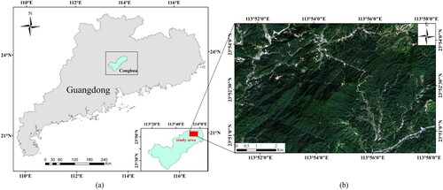
The study was conducted in the subtropical forest areas situated in north-eastern Conghua, Guangdong province, China. The area covering the extent of the airborne LiDAR data acquisition is geographically located between latitude 23°50′9″ to 23°55′1″N and longitude 113°50′57″ to 113°58′36″E (Figure 1). The elevation ranges from approximately 198 m in the northeast to 619 m in the southwest. The climate is subtropical monsoon, with yearly mean temperature of 21.3 °C and yearly mean rainfall of 1952.4 mm, and the rainy season lasts from April to September. The main vegetation types in this study site are broadleaf and coniferous mixed forest and the dominant tree species include Pinus massoniana, Schima superba, Cinnamomum porrectum, and Castanopsis fissa.

Figure 1. Study area. (a) Mapping showing the study site location in Conghua, Guangdong province, China; (b) S-2 image of the study site obtained on 27 October, 2017.

2.2. Field data

The field campaigns were conducted from August to September 2017. There were 60 sample plots in total, and each plot was square in shape with an area of 30 m × 30 m. The plot positions covered by the extent of LiDAR flights were selected on the basis of a subjective assessment. The centers of these plots were recorded using a GPS (Garmin MAP 60CS, accuracy ±3 m), and the tree species, along with the corresponding type (deciduous vs. evergreen), were also taken down. At each field plot, all the measurements (e.g. DBH and H) indispensable for calculating biomass were obtained. Furthermore, all the trees with a DBH <3 cm were abandoned during the measurements. The vegetation type (i.e. coniferous, deciduous, or mixed forest) of each plot was determined via a threshold of 75% in advance of the analysis (Singh et al. 2015). If deciduous (coniferous) trees accounted for more than 75%, the vegetation type of the plot would be marked as deciduous (coniferous), otherwise, it would be marked as mixed forest (Godwin, Chen, and Singh 2015).

In this study, we followed the methodology of Fang, Liu, and XU (1996) for biomass accounting in each plot. On the basis of the DBH and H, the volume of every tree was acquired through a volume table. Then, the summation of each tree volume was obtained as the total volume (TV) at plot scale. The total AGB (TAGB) in each plot was calculated using the relationship (Eq. 1(1) $TAGB=\mathrm{a}\times \mathrm{TV}+\mathrm{b}$(1) ) between the TV and TAGB: (1) $TAGB=\mathrm{a}\times \mathrm{TV}+\mathrm{b}$(1) where a and b are known constants from Fang, Liu, and XU (1996), and their values hinge on the forest types of the plots. The plot biomass was ultimately obtained at a megagrams per hectare (Mg/ha) conversion unit. The on-site plots covered a broad spectrum of AGB values ranging from 17.58 Mg/ha to 278.443 Mg/ha, with an average value of 125.732 Mg/ha and a standard deviation of 71.13 Mg/ha.

2.3. Data collection and pre-processing

2.3.1. LiDAR data collection and pre-processing

Airborne LiDAR data were acquired in June 2017 using the fixed-wing aircraft PartenaviaP68 at a mean height of 850 m above the ground and a maximum scan angle of 15°. The data were collected along twelve survey transects with a width of approximately 300 m. A maximum of two echoes each laser pulse was recorded by the two-return range detection LiDAR system. The pulse frequency was approximately 70 kHz, and the average density was approximately 1.5 pulses/m². The raw point cloud data preprocessing was completed using Terrascan software (v4.006-Terrasolid, Helsinki, Finland). The LiDAR data were pre-processed by first recognizing and removing individual noisy points. We classified the point cloud data into two categories ground and non-ground returns, and then the interpolation procedure was separately conducted for the ground returns and all first returns in order to produce a digital surface model (DSM) and a DEM with a 1 m resolution. To obtain the crown height model (CHM) raster data, the DEM was subtracted from the DSM. The CHM pixels with values between 2 and 35 m were reserved based on the maximum and minimum of measured tree heights within this area to remove the undergrowth vegetation and objects above the height of the trees (Hyyppa et al., 2012; Wulder et al. 2012).

2.3.2. Satellite data acquisition and pre-processing

Two satellite image types (i.e. S-1 and S-2) were utilized in this study. According to previous studies, the integrated use of SAR and optical images could improve the estimation performance of the vegetation parameters (Castillo et al. 2017; Forkuor et al. 2020). Due to the near independence of S-1 data from weather circumstances, in the instances of excessive cloud cover, S-2 could not provide available data, and the S-1 imagery can be used to fill the gap. S-2 data, which have three red-edge bands related to vegetation information, are frequently used high-resolution data for large-scale AGB mapping. S-2 has a 5-day temporal resolution. The potential of S-2 data to augment the AGB prediction has been shown by several studies (Puliti et al. 2020; Theofanous et al. 2021). However, the S-2 image is often susceptible to cloud cover, and integrating S-1 and S-2 provides year-round images to improve the estimation accuracy.

S-1 images for the period from January to December 2017 were obtained from the Google Earth Engine (GEE) (https://code.earthengine.google.com) (Figure 2). The S-1 data were gathered in the Interferometric Wide Swath (IW) mode with the VV (Vertical transmit -Vertical receive) and VH (Vertical transmit -Horizontal receive) polarizations, and they were the Multi-Look Ground Range-Detected (GRD) products. Twelve scenes (a scene monthly) covering the study site were acquired. In this study, the API interface based on JavaScript language was used to load the GRD product dataset, i.e. ‘COPERNICUS/S1_GRD’, in the ‘Code Edit’ module of the GEE platform. The dataset was pre-processed for each scene using ESA's Sentinel Applications Platform (SNAP) software, including orbit files applying, thermal noise processing, speckle filtering, radiometric calibration, terrain correction, and geocoding. Therefore, the processed data (i.e. backscatter coefficients) completed by GEE could be used directly. Subsequently, all the S-1 data were resampled to 10 m resolution using the bilinear interpolation method and resized based on the spatial coverage of the study site.

Figure 2. Calendar of the Sentinel-1 and Sentinel-2 data acquisitions.

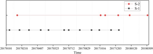
S-2 images were obtained from the Copernicus Open Access Hub (https://scihub.copernicus.eu/dhus/#/home). S-2 data were acquired for the months of January, February, March, October, November and December 2017 (Figure 2). Owing to an excess of cloud coverage for a considerable part of the study site, the other months of 2017 failed to provide effective data. For each image, atmospheric correction was implemented by employing the Sen2cor plugin of SNAP version 9.0 software (SNAP 2022) to transform the Level 1C to Level 2A. The coastal aerosol, water vapour, and SWIR-Cirrus bands were abandoned due to their contribution to atmospheric correction and lower spatial resolution, with ten spectral bands remaining. Three red-edge bands, one near infrared (NIR) band, and two short-wavelength infrared (SWIR) bands of 20 m resolution were resampled using the bilinear interpolation approach to a spatial resolution of 10 m. Each S-2 image was clipped to cover the study region precisely.

3. Methods

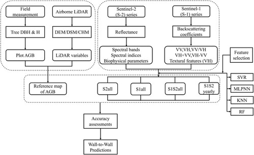
Figure 3 illustrates the proposed method for forest AGB estimation in the study. Five major steps were followed to acquire the AGB map: (1) predictors extraction, (2) reference map of AGB establishment, (3) training and testing datasets production, (4) feature selection procedure and (5) model calibration and assessment.

Figure 3. The workflow of the proposed approach for the modeling and mapping of the subtropical forest AGB.

3.1. Predictors extraction

3.1.1. LiDAR variables

Two classes of LiDAR variables were derived: the canopy height and canopy cover metrics (Table 1). Three types of canopy height variables describing the distribution condition of heights were calculated, including the percentile height (H.p: p60, 70, 80, 90, and 95), mean height (H._mean), and interquartile distance of percentile height (HIQ). For the canopy cover variables, the point densities (PD), which were of diverse height intervals (such as the proportion of returns above 10 m or between 10 and 20), were derived (Almeida et al. 2019). The whole area along the LiDAR transects was resampled to 10 m, and the 14 LiDAR variables were extracted for every cell.

Table 1. List of LiDAR variables for AGB estimation.

LiDAR variables	abbreviation	Definition	Reference
Height	H.mean	Mean height.	Qin et al. (2022)
	H.pX	X^th (60,70,80,90, or 95) percentile.	Almeida et al. (2019)
	HIQ	Interquartile distance of percentile height, H75th – H25th.	Wang et al. (2020)
Canopy cover	PDh	Number of first returns above a height h (10, 14, 18, 22, or 26) divided by the amount of all first returns.	Almeida et al. (2019)
	PDa_b	Number of first returns between the height interval a_b (10_20, or 20_30) divided by the amount of all first returns.	Almeida et al. (2019)

3.1.2. Sentinel-2 and Sentinel-1A variables

Three classes of optical variables were derived from the pre-processed Sentinel-2 images: spectral bands, vegetation indices, and biophysical parameters (Table 2). The red, green, blue, red-edge, near-infrared, and SWIR bands were employed for subsequent analysis. For each scene, nine spectral indices were chosen based on previous research (Castillo et al. 2017; Wang et al. 2020; Wu et al. 2022) (Table 2). In addition to the vegetation indices, three biophysical parameters, including FAPAR, FVC, and leaf area index (LAI), were derived for all the images. These biophysical metrics were shown to be sensitive to forest AGB due to their description for vegetation status and dynamics information (Forkuor et al. 2020; Ronoud et al. 2021). This step was performed for each scene by the biophysical processor of the SNAP software. The processor derived biophysical parameters using tested, general approaches based on PROSAIL radiative transfer model.

Table 2. The list of variables extracted from S-1 and S-2 images.

Source image		Bands, indices or parameters	Definition
S-1(monthly: January to December 2017)	Polarization/channel	VH	Vertical transmit-horizontal channel
		VV	Vertical transmit-vertical channel
	Indices	VV / VH	Quotient
		VH + VV	Sum
		VH – VV	Difference
	Textural Features	Mean	${\sum }_{i,j=0}^{N=1}i{P}_{i,j}$
		Homogeneity	${\sum }_{i,j=0}^{N-1}i{\displaystyle \frac{P_{i,j}}{1+{(i-j)}^2}}$
		Variance	${\sum }_{i,j=0}^{N-1}{P}_{i,j}(1-{\mu }_i)$
		Contrast	${\sum }_{i,j=0}^{N-1}i{P}_{i,j}{(i-j)}^2$
		Entropy	${\sum }_{i,j=0}^{N-1}i{P}_{i,j}(-\ln P_{i,j})$
		Dissimilarity	${\sum }_{i,j=0}^{N-1}i{P}_{i,j}|i-j|$
		Second moment	${\sum }_{i,j=0}^{N-1}i{P}_{i,j}^2$
		Correlation	${\sum }_{i,j=0}^{N-1}{\displaystyle \frac{(i-Mean)(j-Mean)P_{i,j}^2}{Variance}}$
S-2 (January, February, March, October, November, December 2017)	Spectral Bands	B2	Blue, 490 nm
		B3	Green, 560 nm
		B4	Red, 665 nm
		B5	Red edge, 705 nm
		B6	Red edge, 749 nm
		B7	Red edge, 783 nm
		B8	Near Infrared (NIR-1), 842 nm
		B8A	Near Infrared (NIR-2), 865 nm
		B11	SWIR-1, 1610 nm
		B12	SWIR-2, 2190 nm
	Spectral Indices	NDVI	(Band8–Band4)/(Band8 + Band4)
		EVI	[2.5*(Band8 – Band4)]/[Band8 + 6*Band4 - 7.5*Band2 + 1]
		TNDVI	[(Band8 – Band4)/(Band8 + Band4) + 0.5]^1/2
		IRECI	(Band7 – Band4)/(Band5/Band6)
		NDVIre1	(Band8 – Band5)/(Band8 + Band5)
		NDVIre2	(Band8 – Band6)/(Band8 + Band6)
		NDVIre3	(Band8 – Band7)/(Band8 + Band7)
		MDI1	(Band8 – Band11)/Band11
		MDI2	(Band8 – Band12)/Band12
	Vegetation Biophysical Variables	LAI	Leaf Area Index
		FVC	Fraction of Vegetation Cover
		FAPAR	Fraction of Absorbed Photo-synthetically Active Radiation

According to published studies (Bhatt and Nain 2021; Forkuor et al. 2020; Mayamanikandan et al. 2022), two polarization bands (VH, VV), the quotient (VV/VH), the sum (VH + VV), and the difference (VH-VV) were calculated as the SAR inputs. Furthermore, research based on texture measures has shown good potential to predict forest structure parameters (Chen et al. 2018; Liao, He, and Quan 2020; Thapa et al. 2015). Eight texture features comprising the mean, homogeneity, variance, dissimilarity, second moment, entropy, contrast, and correlation, were produced from the radar backscatter band (VH) based on the grey level co-occurrence matrices (GLCM) (Table 2). The superiority of texture features extracted from small window sizes to fine changes in pixel brightness compared with those computed from a large window size had been shown (Kelsey and Neff 2014). Therefore, we selected a 3 × 3 window size to acquire texture variables. Table 2 shows a list of all the variables (metrics extracted from S-1 and S-2 data) employed in the study.

3.2. Reference map of AGB

The 60 field-measured AGB values were randomly split into 70-30% training and testing samples. Based on the biomass measurements and LiDAR variables (Table 1), AGB modeling was implemented using the SVR method. The computational complexity of SVR algorithm does not depend on the dimensionality of the sample space, which avoids the curse of dimensionality at some level. Moreover, it is impervious to outliers and thus has relatively better robustness. In Chen et al. (2018), the SVR model reached the best performance for AGB prediction using limited field data.

To reduce the information redundancy and improve the efficiency during AGB retrieval, the backward feature exclusion method was performed to filter the LiDAR variables sensitive to biomass. When removing a metric leads to a decrease in the RMSE value of the SVR model, it means that this variable contributes little to AGB, and vice versa. The optimal group of LiDAR variables was obtained when the RMSE no longer decreased, and then they were utilized for AGB prediction, thereby forming the LiDAR-derived AGB reference map with 10 m spatial resolution.

3.3. Training and testing data

288 variables in total were utilized to estimate forest AGB. The selected predictors consisted of 60 S-2 optical bands (10 spectral bands each from six images), 54 S-2 vegetation indices, 18 S-2 biophysical metrics, 24 SAR polarization bands (2 bands each from 12 scenes), 36 SAR difference, quotient, sum bands, and 96 texture features. 660 samples that were almost evenly distributed within the AGB reference map were adopted (Table 3). The number of samples selected based on the extent of the region (100 km²) was comparable to that in similar studies (Shao, Zhang, and Wang 2017). The extracted biomass values from the AGB reference map were appended to the calculated backscatter and optical information. The total samples were randomly divided into training and testing samples at a ratio of 7:3.

Table 3. Summary of the AGB values of 660 samples (Mg/ha).

Range	19–85	86–150	151–217	218–264
Number of plots	159	179	164	158
Sum	660
	Range	Mean		Standard deviation
	34.48-256.71	145.73		51.27

3.4. Regression algorithms

In our study, four diverse regression methods including SVR, MLPNN, KNN, and RF were considered to map AGB. An introduction of each algorithm is provided as follows.

With the support vector machine (SVM), regressions are accomplished depending on the major principle that mapping the input vector to a high-dimensional feature space using some well-chosen nonlinear mapping kernel function (Almeida et al. 2019). SVM comprises three diverse implementations, namely, SVR, NuSVR, and LinearSVR. The SVR method was selected because it is frequently used. The SVR method is derived from the support vector classification method. The Gaussian Kernel, namely, radial basis function (RBF), was chosen to predict forest AGB. Many studies have compared different kernels and the superiority of RBF kernel was found (Monnet, Chanussot, and Berger 2011; Nguyen et al. 2020). The SVR (RBF) was further optimized by using the gird search approach to detect a more appropriate combination of C and epsilon that maximized the R². C is a regularization parameter. Epsilon specifies an epsilon-tube whose training loss function has no penalty related to points forecasted within a distance epsilon from observed values. The SVR algorithm has demonstrated the superiority of the generalization ability (Monnet, Chanussot, and Berger 2011).

Figure 4. Schematic diagram of an instance MLPNN model structure to estimate forest AGB. The neurons N_i, N_j, N_k in the input layer, hidden layers, and output layer, as well as their internal connections and weightings (W_ij, W_jk) were shown.

Figure 4. Schematic diagram of an instance MLPNN model structure to estimate forest AGB. The neurons N_i, N_j, N_k in the input layer, hidden layers, and output layer, as well as their internal connections and weightings (W_ij, W_jk) were shown.

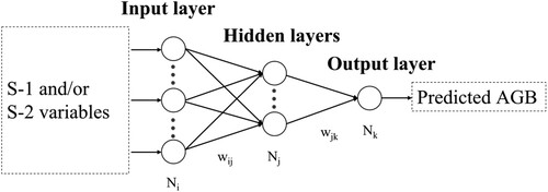
MLPNN is a non-parametric algorithm. The rationale of the neural network is to simulate and facilitate biological neurons, and multi-layer perceptron (MLP), which is the most fundamental neural network model, was used in this research (Chen et al. 2018). With the exception of an input layer and an output layer, at least one hidden layer is incorporated into MLP, and its different layers are fully connected (Figure 4). The training method generally adopts the backpropagation (BP) algorithm. Compared to single-layer perceptron, multi-layer perceptron can learn nonlinear functions. The regression model was optimized by looking for appropriate activation functions, along with the number of hidden layers and nodes. The MLPNN method has been demonstrated to be a feasible algorithm for estimating AGB (Chen et al. 2018).

For K-nearest neighbour (k-NN) algorithm, the main idea is that the estimated value of each query point to be measured is acquired via the weighted average of the corresponding attribute values of the k nearest neighbours (Xie et al. 2022). Uniform was selected as a weight parameter because each point in the local neighbourhood contributes equally to uniform weights in the prediction of a query point. This characteristic is suitable for our datasets. The parameters n_neighbours and leaf_size of KNN were set to keep the default values. The advantages of the KNN algorithm have been proven (for example, in terms of their effectiveness and convenience) (Persson, Jonzén, and Nilsson 2021).

RF is considered the most frequently used and efficient algorithm. It belongs to the ensemble learning method, which is approximately divided into bagging and boosting methods (Almeida et al. 2019). The general idea behind ensemble learning is to train many relatively weak models (e.g. decision tree, SVM, etc.) and package them to yield a relatively strong model (Forkuor et al. 2020). The strong model outperformed a single weak model. Decision trees are used as weak models in RF. During the training phase, RF employ bootstrap sampling to gather many diverse sub-training sets from the input training set for training multiple diverse decision trees in turn. The aim of using bootstrap sampling is to utilize multiple diverse sub-models to augment the robustness and stability of the final models. In the prediction phase, the RF predicts a response variable by averaging the results predicted by multiple interior decision trees to acquire the final outcome. In this study, RF was optimized by using the gird search approach to explore the more proper combination of a number of trees (ntree) and depth of trees (mdepth) to improve the performance. Moreover, the previous research (Zald et al. 2016) supported the superiority of the RF which has no demand for the feature dimension of the dataset compared with the other machine learning algorithms.

3.5. Experimental design

Consistent with this study’s purpose, four experiments were implemented with diverse datasets to estimate forest AGB: (1) all optical data; (2) all SAR data; (3) yearly time-series of SAR and optical data; and (4) the integration of all SAR and optical data. Table 4 presents the details about the experiments. The modeling framework was built by applying the four datasets to the four prediction models (RF, KNN, SVR, and MLPNN). Prior to modeling, a feature selection procedure was used to acquire the optimal predictors for each model. Section 3.6 details the variable selection method used here.

Table 4. Experimental design for AGB estimation.

Experiment	Abbreviation	Amount of predictors	Objective/description
A: All S-2 data	S2all	132	Spectral bands, vegetation indices and biophysical parameters for six months – Jan., Feb., Mar., Oct., Nov. and Dec.
B: All S-1 data	S1all	156	Yearly time-series polarization bands and corresponding texture features, sum, difference and quotient bands
C: Yearly time-series of S-1 and S-2 data	S1S2yearly	210	S-1 data was utilized to fill-in for the months when S-2 data failed.
D: All S-1 and S-2 data	S1S2all	288	All obtained optical and SAR predictors

3.6. Feature selection

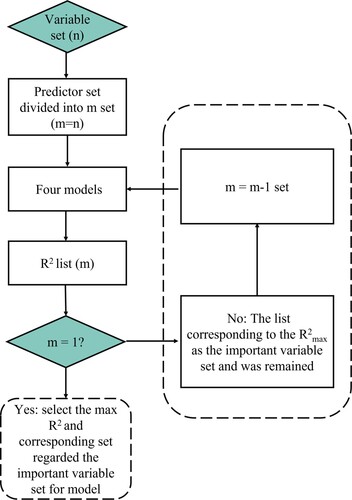
The aim of this step was to detect the optimal predictors of each model for estimating AGB. For this objective, we employed the sequential procedure to eliminate comparatively inferior predictors using the LiDAR-derived AGB value as the independent testing dataset (N = 198). The model performance was evaluated by the coefficient of determination (R²). The sequential forward selection (SFS) began with an available variable to build a prediction model, and then the model was validated using testing samples of the corresponding variable. The predictor that had the highest R² was retained. In the next step, the saved predictor with another variable from the remaining set (n-1) were used to run as the training set, and the model was subsequently validated based on the same principle. The SFS took into account all the potential combinations of variables as much as possible and selected the subset with the maximum R², which meant the predictors having the best contribution to the model were determined (Figure 5). The SFS was applied to each dataset (S2all, S1all, S1S2yearly, and S1S2all), and the selected variables from each dataset were respectively input into the four prediction models (RF, KNN, SVR, and MLPNN).

Figure 5. Flow chart of the sequential forward selection.

3.7. Accuracy assessment

The accuracy of each experiment was evaluated by independent testing samples (N = 198) not involved in the process of model building. Three accuracy evaluation indices (Eq. 2(2) $R^2=1-{\displaystyle \frac{{\sum }_{i=1}^n{(E_i-T_i)}^2}{{\sum }_{i=1}^n{(E_i-T_i)}^2}}$(2) -4) were calculated to contrast the forecasted values with observed values (LiDAR-derived AGB values). They are the coefficient of determination (R²), root mean squared error (RMSE, Mg/ha), and relative RMSE (RMSEr, %) assuming the form of a percentage. (2) $R^2=1-{\displaystyle \frac{{\sum }_{i=1}^n{(E_i-T_i)}^2}{{\sum }_{i=1}^n{(E_i-T_i)}^2}}$(2) (3) $RMSE={\left[n^{-1}\sum _{i=1}^n{(E_i-T_i)}^2\right]}^{1/2}$(3) (4) $RMS{E}_{\mathrm{r}}={\displaystyle \frac{{\left[n^{-1}\sum _{i=1}^n{(E_i-T_i)}^2\right]}^{1/2}}{n^{-1}\sum _{i=1}^n(T_i)}}$(4)

Where ‘E’ is the estimated value, and ‘T’ is the true value.

4. Results

4.1. Performance assessment of the AGB reference map

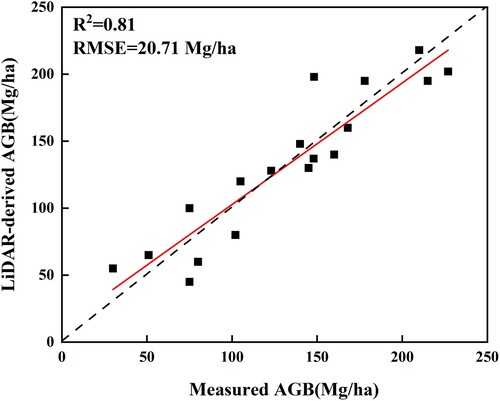
Based on the backward feature exclusion method, the optimal LiDAR variables, including the H._mean, H._p80, H._p90, H._p95, PD_{20_30}, PD₁₄, PD₂₂, and PD₂₆, were applied to produce the AGB reference map. The accuracy of the SVR model validated using the independent testing dataset (18 field-measured AGB) was R² of 0.81 and RMSE of 20.71 Mg/ha (Figure 6). Satisfactory accuracy (R²: 0.81, RMSE: 20.71 Mg/ha) was acquired compared with similar research (Shao, Zhang, and Wang 2017; Tsui et al. 2013), and thus laid a dependable foundation for follow-up modeling work. In the LiDAR-derived biomass map, the AGB values ranged from 19.32–263.74 Mg/ha, with an average value of 132.69 Mg/ha and a standard deviation of 64.81 Mg/ha. The biomass values in the reference map were subsequently utilized as training and testing data for the satellite-based wall-to-wall AGB estimating.

Figure 6. Scatterplot of measured AGB versus LiDAR-derived AGB.

4.2. Performance of diverse data inputs and prediction models for AGB estimation

Table 5 shows the testing outcomes of sixteen experiments implemented with S-1 and/or S-2 data. All of the experiments were assessed using the same independent testing dataset (N = 198). Except for experiment B, the RF model outperformed the other prediction models, and the worst performance was afforded by the SVR model, which delivered a relatively higher RMSE for each experiment. The performance of the KNN and MLPNN models varied in different experiments. For instance, KNN outperformed MLPNN in experiment D, while MLPNN outperformed KNN in experiment C. In terms of all four regression methods, the results in experiments S2all and S1all suggested that S-2 data, which were obtained in six months, assumed better performance compared to the S1all acquired in twelve months in general. Even if the KNN model acquired the best performance with an RMSE of 46.49 Mg/ha compared to other models in experiment B, it was still higher than the worst performance with an RMSE of 37.59 Mg/ha reached by the SVR model in experiment A. With respect to R², coefficients of determination of 0.33 and 0.48 were achieved for S1all in the KNN model and S2all in the SVR model, respectively. The combination of yearly monthly time-series of S-1 and S-2 images improved the estimation accuracy of the models for all the prediction algorithms by increasing the R² and decreasing the RMSE_r. The improvements in the R² (increase of 0.10-0.14) and RMSE_r (decrease of 2.38-4.88%) were reached by experiment S1S2all relative to models with S2all. Relative to the counterpart in experiment S1S2yearly, experiment S1S2all acquired a higher accuracy with four models. Overall, the best performance was afforded by the RF model and experiment S1S2all. The reference AGB versus model predicted AGB derived from the different data sources and methods are plotted in Figure 7. All the models showed an overestimation of low AGB and an underestimation of high AGB. However, the RF model with all optical and SAR data whose points were closer to the 1:1 line compared with the other models showed slight overestimation and underestimation.

Figure 7. The scatterplots of the reference AGB and model predicted AGB produced from the S-1 and/or S-2 sources and diverse methods.

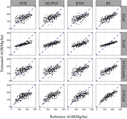
Table 5. Modeling performance for diverse prediction algorithms and data sources.

Data	Algorithm	Features	R^2	RMSE (Mg/ha)	RMSEr (%)
S2all	SVR	4	0.48	37.59	24.90
	MLPNN	38	0.53	35.57	23.56
	KNN	20	0.53	35.86	23.75
	RF	25	0.59	33.21	22.00
S1all	SVR	4	0.21	50.89	33.63
	MLPNN	26	0.32	47.55	31.42
	KNN	90	0.33	46.49	30.72
	RF	37	0.29	48.21	31.86
S1S2yearly	SVR	10	0.55	34.08	21.84
	MLPNN	17	0.61	31.72	20.28
	KNN	91	0.60	31.99	20.46
	RF	17	0.66	29.80	19.01
S1S2all	SVR	20	0.58	33.61	22.53
	MLPNN	17	0.64	31.16	19.91
	KNN	50	0.67	29.32	18.87
	RF	46	0.72	28.63	17.65

4.3. Optimum variables and data acquisition periods for AGB estimation

The most critical predictors selected by the SFS procedure for each model in four experiments are presented in Tables S1-4 (Supplementary). With respect to the amount of selected optimal predictors, the importance of S-1 and S-2 data to the S1S2yearly and S1S2all experiments hinged on the prediction method considered. For the combined experiments (S1S2yearly, S1S2all), the optical variables were selected more than the SAR variables except for the MLPNN model in experiment S1S2all. Moreover, the MDI2 metric was only chosen by the MLPNN method, and the sum, variance, along with the mean predictors, were not selected by any model in combined experiments (S1S2all and S1S2yearly).

The optimal variables and image acquisition period for the RF model assuming the best performance for AGB estimates in each experiment are shown in the predictor importance graphs (Figure 8). Compared with the backscatter bands along with conventional vegetation indices, derivatives such as the texture features (entropy, contrast, and correlation), radar indices, biophysical parameters, and red-edge and shortwave infrared indices were discovered to be preferable variables for AGB estimation in all the experiments. For S1S2yearly and S1S2all, the top four most crucial predictors were the shortwave infrared index (Mar_MDI1), biophysical products (Feb_LAI, Nov_LAI/Oct_LAI), and SAR index (Apr_VHVVc). Among the first ten most contributing predictors, in S1all, texture measures accounted for six out of ten (Dec_variance, Oct_dissimilarity, Jun_correlation, Mar_correlation, Jun_variance, and Jun_homogeneity), and in S2all, the top six most informative metrics were derivatives (Oct_NDVIre1, Mar_LAI, Nov_MDI2, Feb_IRECI, Jan_NDVI, and Jan_IRECI). In addition, the graphs reveal that the quotient indices were more useful for AGB modeling than the difference and sum indices, although the quotient indices were the worst predictor of three SAR indices in S1all. Overall, the biophysical parameters, near-infrared and shortwave infrared indices of optical data, along with the quotient indices of SAR data, were found to contribute more to the AGB prediction.

Figure 8. Importance ranking of the 10 highest predictors for RF model with four different datasets.

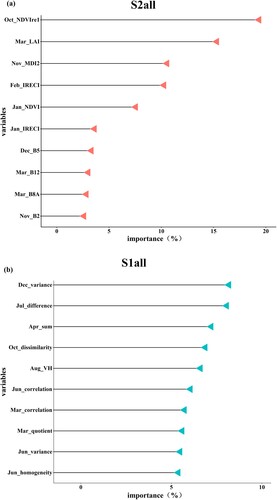
Figure 8. Continued.

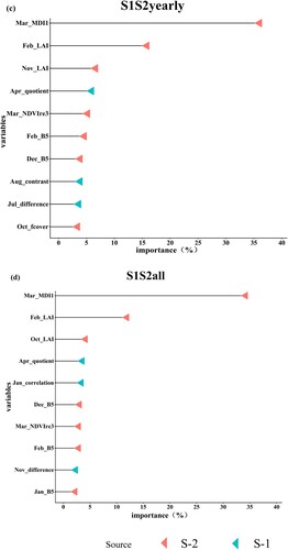
According to the predictor importance ranking of experiments S1all, S1S2yearly, and S1S2all with respect to the RF model (Figure 8), the optimal image acquisition stages for estimating subtropical forest AGB were investigated. The results of ranking in experiment S1S2all revealed that the top ten most important predictors were almost all obtained during the arid periods (October to March), except for one metric (Apr_quotient). In experiment S1all, the most important metric (Dec_variance) was acquired during the arid season. Moreover, the inclusion of arid season SAR data (S1S2all) improved the AGB estimation accuracy compared to the experiment S1S2yearly. Consequently, the images (S-1 and S-2) of arid seasons were important for the subtropical forest AGB estimating in the study site.

4.4. Forest AGB predictive mapping

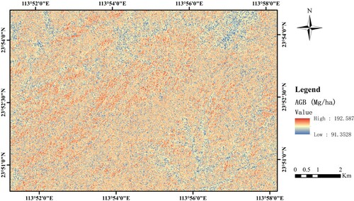
The final AGB map of the study region derived from integrated S-1 and S-2 images (S1S2all) using the RF model is presented in Figure 9. The estimated map is characterized by AGB values ranging from a low of 91.35 Mg/ha to a high of 192.59 Mg/ha, and the average values is 163.95 Mg/ha. Additionally, about 70% of the study region has AGB values between 140 and 170 Mg/ha. The spatial distribution of forest AGB predictions, such as high and low biomass areas, is consistent with field observations. Nevertheless, there was an overestimation or underestimation occurring in sparse or dense forest areas, while the result that approximately 70% of the final AGB map was between 140 and 170 Mg/ha is in line with the study area.

Figure 9. AGB map from the RF model with all the S-1 and S-2 integrated variables (S1S2all).

5. Discussion

5.1. The LiDAR-derived AGB as a substitute for field-measured data

To our knowledge, the AGB reference map derived from LiDAR data and field plots as ground reference data was relatively rarely employed to characterize subtropical forest information. The feasibility of using LiDAR data as a substitute for conventional forest inventories has been demonstrated by previous research (Shao, Zhang, and Wang 2017; Zald et al. 2016). Apart from further confirming the suitability of the LiDAR-derived reference map, the follow-up modeling work which reached satisfactory accuracy (R²: 0.72; RMSE: 28.63 Mg/ha; RMSE_r: 17.65%, for the best model), also demonstrated the applicability of yearly multi-temporal time-series of SAR and multispectral data for AGB mapping. There were trends to overestimate AGB in sparse forests and underestimate AGB in dense forests. The overestimation may be pertaining to the variation of background land cover and undergrowth vegetation, which leads to an increase in spectral variation. Compared to other ground cover, the relationship between spectral information of the background classes and AGB becomes more complicated. The explanation for underestimation could be that saturation phenomena occurs, which is critical limitation for optical data when estimating AGB in dense vegetation areas. The H._mean, H._p80, PD_{20_30}, and other LiDAR variables selected by the backward feature exclusion method were consistent with some similar studies (Almeida et al. 2019; Wang et al. 2020), which indirectly supported the correctness of this routine. Furthermore, the good validation accuracy (R²: 0.81, RMSE: 20.71 Mg/ha) (Figure 6) also demonstrated the reliability of the reference map of AGB as a substitute for ground reference data. The subsequent modeling results indicated that employing the LiDAR-derived AGB as a surrogate for field measurements is relatively economical and reliable, and thus, it can be applied in future studies when the amount of representative inventories in large forest areas is restricted. Despite its superiority, the method had a limitation which requires LiDAR data available.

5.2. S-1 versus S-2 for modeling AGB

The outcomes of our research showed that S-2 data are more applicable for mapping AGB in the study site than S-1 data. Although this discovery is consistent with previous studies comparing the contribution of SAR and optical data in estimating AGB (Forkuor et al. 2020; Vafaei et al. 2018), others presented inverse results (Chen et al. 2018; Navarro et al. 2019). This result can be attributed to the short wavelength (C-band), which has a limited ability to capture vertical structural information of forests compared with longer wavelength SAR images (e.g. L and P). Previous studies have found that the involvement of interferometric synthetic aperture radar (InSAR) can weaken the saturation effect to some degree (Saatchi et al. 2011). Thiel and Schmullius (2016) utilized P-band PolSAR and dual antenna X-band InSAR data to estimate AGB and found that the inclusion of more dimensional SAR features obtained more precise results than unidimensional SAR metrics. The contribution of textural information based on S-1 for AGB mapping has been found both in this study and Chen et al. (2018). Furthermore, our study observed the SAR indices of sum, difference, and quotient (Table 2) to be beneficial for AGB modeling, which was in line with the findings of Forkuor et al. (2020) with the exception of the quotient. Therefore, the SAR indices, textural information, and longer wavelength SAR data (e.g. L- and P bands) coupled with vegetation height information from InSAR should be applied for AGB mapping in the near future.

Although there was a saturation phenomenon with optical data, especially in dense vegetation areas, the performance of S-2 data was still better than the S-1 data in the study. Similar results were reported in other research that compared SAR and optical data to predict AGB. Forkuor et al. (2020), for instance, compared S-1 and S-2 for forest AGB prediction and acquired preferable estimation accuracy with S-2 data (multispectral bands, spectral indices, and biophysical parameters) (R²: 0.83, RMSE: 60.6 Mg/ha, for the S2 model; R²: 0.61, RMSE: 86.6 Mg/ha, for the S1 model). Besides the relatively high spatial resolution and multiple red-edge bands of S-2, the scholars regarded the inclusion of S-2 extracted biophysical variables as functional for the results of S-2. In our study, the involvement of S-2 derived spectral indices, such as NDVIre3 and MDI1, along with biophysical variables (LAI, FAPAR, and FVC), made S-2 as conducive to the estimation performance as possible. Although the contribution of these parameters has been observed by other research (Wang et al. 2020), the importance ranking graphs of experiments S1S2yearly and S1S2all offer new perspectives for the importance and sensitivity of S-2 derived SWIR indices, red-edge indices and biophysical parameters to AGB estimates in the study region. The SWIR indices (MDI1) and biophysical parameters (LAI) were in the top three important predictors in experiments S1S2yearly and S1S2all. The fifth most important variable in experiment S1S2yearly was red-edge indices (NDVIre3). The results of importance ranking graphs further demonstrate the superiority of SWIR indices, red-edge indices and biophysical parameters for AGB estimation in subtropical forest areas.

The combination of SAR and optical data obtained the best results compared to the other experiments implemented here. Similar outcomes were acquired in other studies using SAR and optical data (Forkuor et al. 2020; Shao, Zhang, and Wang 2017). This finding can be attributed to the complementarities of both data in the data characteristics and imaging technique, and thus combining two types of data is conducive to predicting AGB. Furthermore, the integration of yearly monthly time-series of SAR data and optical data according to different seasons provides novel insights for the combination of S-1 and S-2 for future forest AGB estimation. In our study, experiments S1S2all (R²: 0.72; RMSE: 28.63 Mg/ha; RMSE_r: 17.65%, for the best S1S2all model), along with S1S2yearly (R²: 0.66; RMSE: 29.80 Mg/ha; RMSE_r: 19.01%, for the best S1S2yearly model), accomplished the most satisfactory estimation results compared to the other experiments. However, the performance of experiment S1S2all was better than that of S1S2yearly. A possible explanation for this result is the augmentation of derivative information from S-1 data (e.g. texture metrics, quotient, difference, etc.) during the dry season. Therefore, for the study area, the AGB mapping precision is better when as many S-1 derivative features in the dry period as possible are used.

5.3. Performance of SVR, MLPNN, KNN, and RF prediction algorithms

The superior performance of the RF approach has been revealed by many previous studies (Chen et al. 2018; Wang et al. 2020). Chirici et al. (2020) utilized four approaches to yield a wall-to-wall map of growing stock volume and the RF method acquired the best estimation result (R²: 0.69, RMSE_r: 37.2%) compared to the other methods (multiple linear regression, KNN, and GWR). Another study conducted by Fassnacht et al. (2014) applied five methods, including stepwise linear regression, SVR, RF, KNN, and gaussian processes, to estimate biomass, and these methods were selected on the basis of a systematic review of the accessible literature. The outcomes showed that the experiment using the RF method produced the best accuracy (R²> 0.6 and RMSE < 40 t/ha). For this study, the lowest error of AGB estimation (R²: 0.72, RMSE_r: 17.65%, for the best model) was also generated by the RF algorithm in almost all experiments. The satisfactory performance of RF model can be attributed to the robustness and flexibility in terms of noise and outliers. The performance of the KNN and MLPNN changed in different experiments. For example, KNN performed better than MLPNN in experiment S1all, while the opposite outcomes appeared in experiment S1S2yearly. This phenomenon may be caused by the combination of feature selection and data source, and the result of feature selection is related to the characteristics of the model. The reason why the SVR model obtained the worst performance may be that the selected kernel function was not suitable for the input data. The performance of different kernel functions should be determined in future AGB estimations. Aside from picking an appropriate regression method, diverse variable subsets attuned to different models were delivered through the feature selection procedure, which reduced the feature dimension, decreased information redundancy, and improved the modeling efficiency. The satisfactory results suggested the feasibility of our feature selection procedure. Other feature selection approaches should be investigated in follow-up studies to improve the AGB modeling performance.

5.4. Contribution of S-1 and S-2 derivatives in estimating AGB

The importance ranking graphs suggested that on the whole, derivatives of S-1 and S-2 data are preferable for predicting AGB than the original information (backscatter and spectral bands). Similar results were found by other studies using SAR and optical data to estimate AGB (Castillo et al. 2017; Forkuor et al. 2020). For instance, Forkuor et al. (2020) found that backscatter indices (S-1), spectral indices, and biophysical parameters (S-2) were more efficient than multispectral (S-2) and backscatter (S-1) bands in mapping AGB. Castillo et al. (2017) conducted a total AGB estimation study on diverse coastal land uses and found that the model based on LAI (S-2) had a higher accuracy than that using the raw bands (S-1 and S-2) and the vegetation indices. They observed the importance of using derivatives. In reference to S-1, valuable information was provided by extracted indices of the difference (VV-VH) and quotient (VH/VV), along with textural features of correlation and contrast in this study. The quotient indices were more important variables than the difference in the S1S2all and S1S2yearly experiments. Overall, the S-1 derivatives contribute more than the raw backscatter bands.

In the case of S-2, the vegetation indices MDI1 and NDVIre3 were shown to be the optimal predictors for AGB estimates in the study. MDI1 was noted to be the most important metric rather than the other red-edge derived spectral indices, followed by the biophysical predictors (LAI) in the S1S2all and S1S2yearly experiments. Wang et al. (2020) acquired similar results and found that MDI1 was as important a predictor for AGB modeling after variable selection. The effectiveness of both NIR bands and SWIR bands in AGB mapping was further verified by this research. This knowledge notwithstanding, the performance of MDI2, which was excluded from the variable set after predictor selection in experiments S1S2all and S1S2yearly concerning the RF method, was inferior to MDI1. On the other hand, the potential of red-edge derived spectral index NDVIre3 was observed, which can be attributed to its capacity to relieve the saturation problem in AGB mapping. This finding is in line with previous research which used red-edge derived vegetation indices for AGB estimation (Mutanga and Skidmore 2004). Concerning biophysical parameters, this study suggested that LAI had better performance than the other two (FVC, FAPAR). The results were in line with those observed by Chen et al. (2018), who used the LAI, FAPAR, and FVC for estimating AGB, and they detected a higher correlation between AGB and LAI. However, Baloloy et al. (2018) observed a relatively lower correlation for LAI in AGB estimation, and Forkuor et al. (2020) also revealed that the LAI made a lower contribution compared to FAPAR and FVC. The reason for these differences may be attributed to the distinctions in the vegetation structure and density. For example, there was poor forest cover for the study area in Forkuor et al. (2020), while Chen et al. (2018) and our study regions had relatively higher stand density with a mean AGB value of more than 100 Mg/ha.

5.5. Influence of seasonality on model performance

Concerning the influence of seasonal factors, the graphs of predictor importance ranking delivered by the RF model for the four experiments revealed that data obtained in the arid period (October to March) contribute to AGB estimation in this study region. Bouvet et al. (2018) and Laurin et al. (2013) observed that the sensitivity of SAR images to AGB is susceptible to seasonal factors. The increase in vegetation and surface moisture during the rainy season could lead to the reduced sensitivity of SAR images to AGB (Nguyen et al. 2016). S-1 with relatively low canopy penetration compared to P- and L-bands could be more suitable for the area with a great percentage of deciduous vegetation where the branches could be emerged in the arid period (Laurin et al. 2013). By comparing experiments C with D, it is also clear that the inclusion of SAR data during the dry season enhanced the model performance. The findings on seasonality in our study coincide with those of Forkuor et al. (2020), who utilized S-1 data to establish a prediction model of the forest AGB in the Sudanian Savanna (SS) agroclimatic region of West Africa. They analysed the variable importance ranking including both arid and rainy season data and they found that the selected SAR variables were all in the arid season, among the top ten optimal features. Overall, when time-series optical and SAR data are combined to predict subtropical forest AGB where optical data available during the rainy season are difficult to obtain, the inclusion of SAR data during the dry season can improve the estimation accuracy.

6. Conclusion

In this study, we determined the potential of integrating LiDAR-derived biomass with the combination of yearly multi-temporal (monthly) time-series of Sentinel-1 (SAR) and Sentinel-2 (multispectral) for estimating subtropical forest AGB in north-eastern Conghua, Guangdong province, China. Four experiments that included diverse feature combinations were designed, and four prediction models (RF, SVR, KNN, and MLPNN) were used for our objectives. We drew the following conclusions from the study. First, the reference AGB map derived from LiDAR with the synergy of yearly time-series of S-1 and S-2 images yielded satisfying estimation performance (R²: 0.72, RMSE: 28.63 Mg/ha, RMSE_r: 17.65%) for the forest AGB. This scheme provides a potential alternative for large-scale mapping of forest structure attributes when field data are limited and multi-month optical and SAR images are available. Second, the experiment of monthly S-2 (S2all) accomplished preferable precision for AGB mapping compared to that using all the S-1 data (S1all), despite the supplementary use of the two data types (S1S2yearly, S1S2all) obtaining the best performance. Moreover, all the optical and SAR data (S1S2all) outperformed the yearly time-series of the optical and SAR data (S1S2yearly). Regardless of the prediction method used here, the AGB mapping accuracy was improved by at least 9% with regard to the RMSE and RMSE_r after using all the data (S1S2all) relative to all the optical data (S2all). Third, the RF model presented the best performance compared to the other algorithms in this study, which further demonstrates the flexibility and robustness of the RF algorithm. Fourth, the most highly contributing Sentinel-1 variables for AGB mapping were related to the backscatter indices (e.g. quotient, difference, etc.) and texture features (e.g. correlation, contrast, etc.), and the most important Sentinel-2 variables were regarded as the MDI1, LAI, and NDVIre3. Finally, dry season data are sensitive for the AGB estimation of subtropical forests, and rainy season data are also indispensable. This research was devoted to determining the capability for synergy of airborne LiDAR and yearly monthly time-series of SAR and multispectral data for AGB estimation and a satisfying result was obtained. Overall, the proposed methodology provides important insights for low-cost, large-scale, and high-precision structural attribute monitoring in subtropical forest areas.

Acknowledgments

The authors are grateful to the European Space Agency for open data policy. We acknowledge financial support in part by the National Natural Science Foundation of China under Grant 42171439, in part by the Shandong Provincial Natural Science Foundation, China, under Grant ZR2019QD010, in part by the Qingdao Science and Technology Benefit the People Demonstration and Guidance Program, China, under Grant 22-3-7-cspz-1-nsh, in part by the Open Research Fund Program of LIESMARS under Grant 19R07, in part by the Open Research Fund Program of Key Laboratory of Ocean Geomatics, Ministry of Natural Resources, China, under Grant 2021B03, and in part by the Introduction Plan of High-end Foreign Experts under Grant G2021025006L.

Disclosure statement

No potential conflict of interest was reported by the author(s).

Data availability statement

The data that support the findings of this study are available on request from the Xiaoxue Zhang ([email protected]). The data are not publicly available due to privacy.

Additional information

Funding

This work was supported by the National Natural Science Foundation of China; under Grant 42171439; Shandong Provincial Natural Science Foundation, China, under Grant ZR2019QD010; Qingdao Science and Technology Benefit the People Demonstration and Guidance Program, China, under Grant 22-3-7-cspz-1-nsh; Open Research Fund Program of LIESMARS under Grant 19R07; Open Research Fund Program of Key Laboratory of Ocean Geomatics, Ministry of Natural Resources, China, under Grant 2021B03; and Introduction Plan of High-end Foreign Experts under Grant G2021025006L.

References

- Almeida, C.T.d., L. S. Galvão, L.E.d.O.C.e. Aragão, J. P. H. B. Ometto, A. D. Jacon, F.R.d.S. Pereira, L. Y. Sato, et al. 2019. “Combining LiDAR and Hyperspectral Data for Aboveground Biomass Modeling in the Brazilian Amazon Using Different Regression Algorithms.” Remote Sensing of Environment 232: 111323. doi:10.1016/j.rse.2019.111323.
- Baloloy, A. B., A. C. Blanco, C. G. Candido, R. J. L. Argamosa, J. B. L. C. Dumalag, L. L. C. Dimapilis, and E. C. Paringit. 2018. “Estimation of Mangrove Forest Aboveground Biomass Using Multispectral Bands, Vegetation Indices and Biophysical Variables Derived From Optical Satellite Imageries: Rapideye, Planetscope and Sentinel-2 ISPRS Annals of the Photogrammetry.” Remote Sensing and Spatial Information Sciences, 29–36. doi:10.5194/isprs-annals-IV-3-29-2018.
- Bhatt, C. K., and A. S. Nain. 2021. “Estimation of Biophysical Parameters of Rice Using Sentinel-1A SAR Data in Udham Singh Nagar (Uttarakhand).” Mausam 72 (4): 739–748. doi:10.54302/mausam.v72i4.3544.
- Bjork, S., S. N. Anfinsen, E. Naesset, T. Gobakken, and E. Zahabu. 2022. “On the Potential of Sequential and Nonsequential Regression Models for Sentinel-1-Based Biomass Prediction in Tanzanian Miombo Forests.” IEEE Journal of Selected Topics in Applied Earth Observations and Remote Sensing 15: 4612–4639. doi: 10.1109/jstars.2022.3179819.
- Bolton, D. K., N. C. Coops, and M. A. Wulder. 2015. “Characterizing Residual Structure and Forest Recovery Following High-Severity Fire in the Western Boreal of Canada Using Landsat Time-Series and Airborne Lidar Data.” Remote Sensing of Environment 163: 48–60. doi:10.1016/j.rse.2015.03.004.
- Bouvet, A., S. Mermoz, T. L. Toan, L. Villard, R. Mathieu, L. Naidoo, and G. P. Asner. 2018. “An Above-Ground Biomass Map of African Savannahs and Woodlands at 25 m Resolution Derived from ALOS PALSAR.” Remote Sensing of Environment 206: 156–173. doi:10.1016/j.rse.2017.12.030.
- Castillo, J. A. A., A. A. Apan, T. N. Maraseni, and S. G. Salmo. 2017. “Estimation and Mapping of Above-Ground Biomass of Mangrove Forests and Their Replacement Land Uses in the Philippines Using Sentinel Imagery.” ISPRS Journal of Photogrammetry and Remote Sensing 134: 70–85. doi:10.1016/j.isprsjprs.2017.10.016.
- Chen, L., C. Y. Ren, B. Zhang, Z. M. Wang, and Y. B. Xi. 2018. “Estimation of Forest Above-Ground Biomass by Geographically Weighted Regression and Machine Learning with Sentinel Imagery.” Forests 9 (10): 582. doi:10.3390/f9100582.
- Chen, L., Y. Q. Wang, C. Y. Ren, B. Zhang, and Z. M. Wang. 2019. “Optimal Combination of Predictors and Algorithms for Forest Above-Ground Biomass Mapping from Sentinel and SRTM Data.” Remote Sensing 11 (4): 414. doi:10.3390/rs11040414.
- Chirici, G., F. Giannetti, R. E. McRoberts, D. Travaglini, M. Pecchi, F. Maselli, M. Chiesi, and P. Corona. 2020. “Wall-to-wall Spatial Prediction of Growing Stock Volume Based on Italian National Forest Inventory Plots and Remotely Sensed Data.” International Journal of Applied Earth Observation and Geoinformation 84: 101959. doi:10.1016/j.jag.2019.101959.
- Deb, D., J. P. Singh, S. Deb, D. Datta, A. Ghosh, and R. S. Chaurasia. 2017. “An Alternative Approach for Estimating Above Ground Biomass Using Resourcesat-2 Satellite Data and Artificial Neural Network in Bundelkhand Region of India.” Environmental Monitoring and Assessment 189 (11): 12. doi:10.1007/s10661-017-6307-6.
- Delegido, J., J. Verrelst, L. Alonso, and J. Moreno. 2011. “Evaluation of Sentinel-2 Red-Edge Bands for Empirical Estimation of Green LAI and Chlorophyll Content.” Sensors 11 (7): 7063–7081. doi:10.3390/s110707063.
- Drusch, M., U. Del Bello, S. Carlier, O. Colin, V. Fernandez, F. Gascon, B. Hoersch, et al. 2012. “Sentinel-2: ESA's Optical High-Resolution Mission for GMES Operational Services.” Remote Sensing of Environment 120: 25–36. doi:10.1016/j.rse.2011.11.026.
- Fang, J., G. Liu, and S. XU. 1996. “Biomass and Net Production of Forest Vegetation in China.” Acta Ecologica Sinica 16: 497–508.
- Fassnacht, F. E., F. Hartig, H. Latifi, C. Berger, J. Hernández, P. Corvalán, and B. Koch. 2014. “Importance of Sample Size, Data Type and Prediction Method for Remote Sensing-Based Estimations of Aboveground Forest Biomass.” Remote Sensing of Environment 154: 102–114. doi:10.1016/j.rse.2014.07.028.
- Forkuor, G., J.-B. B. Zoungrana, K. Dimobe, B. Ouattara, K. P. Vadrevu, and J. E. Tondoh. 2020. “Above-ground Biomass Mapping in West African Dryland Forest Using Sentinel-1 and 2 Datasets - A Case Study.” Remote Sensing of Environment 236: 111496. doi:10.1016/j.rse.2019.111496.
- “GEE developers forum.”. [Online]. Available: https://developers.google.com/earth-engine/.
- Godwin, C., G. Chen, and K. K. Singh. 2015. “The Impact of Urban Residential Development Patterns on Forest Carbon Density: An Integration of LiDAR, Aerial Photography and Field Mensuration.” Landscape and Urban Planning 136: 97–109. doi:10.1016/j.landurbplan.2014.12.007.
- Han, H. S., R. R. Wan, and B. Li. 2022. “Estimating Forest Aboveground Biomass Using Gaofen-1 Images, Sentinel-1 Images, and Machine Learning Algorithms: A Case Study of the Dabie Mountain Region, China.” Remote Sensing 14 (1): 176. doi:10.3390/rs14010176.
- Hawbaker, T. J., N. S. Keuler, A. A. Lesak, T. Gobakken, and V. C. Radeloff. 2009. “Improved Estimates of Forest Vegetation Structure and Biomass with a LiDAR-Optimized Sampling Design.” Journal of Geophysical Research: Biogeosciences 114: 363–369. doi:10.1029/2008JG000870.
- Hyyppä, J., X.W. Yu, H. Hyyppä, M. Vastaranta, M. Holopainen, A. Kukko, H. Kaartinen, A. Jaakkola, M.T. Vaaja, J. Koskinen, and P. Alho. 2012. “Advances in Forest Inventory Using Airborne Laser Scanning.” Remote Sensing 4 (5): 1190–1207. doi:10.3390/rs4051190.
- Kane, V. R., R. J. McGaughey, J. D. Bakker, R. F. Gersonde, J. A. Lutz, and J. F. Franklin. 2010. “Comparisons Between Field- and LiDAR-Based Measures of Stand Structural Complexity.” Canadian Journal of Forest Research 40 (4): 761–773. doi: 10.1139/x10-024.
- Karki, S., R. Bermejo, R. Wilkes, M. Mac Monagail, E. Daly, M. Healy, J. Hanafin, et al. 2021. “Mapping Spatial Distribution and Biomass of Intertidal Ulva Blooms Using Machine Learning and Earth Observation.” Frontiers in Marine Science 8. doi:10.3389/fmars.2021.633128.
- Kelsey, K. C., and J. C. Neff. 2014. “Estimates of Aboveground Biomass from Texture Analysis of Landsat Imagery.” Remote Sensing 6 (7): 6407–6422. doi:10.3390/rs6076407.
- Kim, J. B., J. M. So, and D. H. Bae. 2020. “Global Warming Impacts on Severe Drought Characteristics in Asia Monsoon Region.” Water 12 (5): 1360. doi:10.3390/w12051360.
- LaRue, E. A., F. W. Wagner, S. L. Fei, J. W. Atkins, R. T. Fahey, C. M. Gough, and B. S. Hardiman. 2020. “Compatibility of Aerial and Terrestrial LiDAR for Quantifying Forest Structural Diversity.” Remote Sensing 12 (9): 1407. doi:10.3390/rs12091407.
- Laurin, G. V., V. Liesenberg, Q. Chen, L. Guerriero, F. Del Frate, A. Bartolini, D. Coomes, B. Wilebore, J. Lindsell, and R. Valentini. 2013. “Optical and SAR Sensor Synergies for Forest and Land Cover Mapping in a Tropical Site in West Africa.” International Journal of Applied Earth Observation and Geoinformation 21: 7–16. doi:10.1016/j.jag.2012.08.002.
- Li, Z.j., Z. Y. Wang, X. T. Liu, Y. D. Zhu, K. Wang, and T. G. Zhang. 2022. “Classification and Evolutionary Analysis of Yellow River Delta Wetlands Using Decision Tree Based on Time Series SAR Backscattering Coefficient and Coherence.” Frontiers in Marine Science 9. doi:10.3389/fmars.2022.940342.
- Li, L., X. S. Zhou, L. Q. Chen, L. G. Chen, Y. Zhang, and Y. Q. Liu. 2020. “Estimating Urban Vegetation Biomass from Sentinel-2A Image Data.” Forests 11 (2): 125. doi:10.3390/f11020125.
- Liao, Z. M., B. B. He, and X. W. Quan. 2020. “Potential of Texture from SAR Tomographic Images for Forest Aboveground Biomass Estimation.” International Journal of Applied Earth Observation and Geoinformation 88: 102049. doi:10.1016/j.jag.2020.102049.
- Lin, J. Y., D. C. Chen, W. J. Wu, and X. H. Liao. 2022b. “Estimating Aboveground Biomass of Urban Forest Trees with Dual-Source UAV Acquired Point Clouds.” Urban Forestry & Urban Greening 69: 127521. doi:10.1016/j.ufug.2022.127521.
- Lin, Y.-C., J. Y. Shao, S.-Y. Shin, Z. Saka, M. Joseph, R. Manish, S. L. Fei, and A. Habib. 2022a. “Comparative Analysis of Multi-Platform, Multi-Resolution, Multi-Temporal LiDAR Data for Forest Inventory.” Remote Sensing 14 (3), doi: 10.3390/rs14030649.
- Liu, Y. A., W. S. Gong, Y. Q. Xing, X. Y. Hu, and J. Y. Gong. 2019. “Estimation of the Forest Stand Mean Height and Aboveground Biomass in Northeast China Using SAR Sentinel-1B, Multispectral Sentinel-2A, and DEM Imagery.” ISPRS Journal of Photogrammetry and Remote Sensing 151: 277–289. doi:10.1016/j.isprsjprs.2019.03.016.
- Lu, D. S., Q. Chen, G. X. Wang, L. J. Liu, G. Y. Li, and E. Moran. 2016. “A Survey of Remote Sensing-Based Aboveground Biomass Estimation Methods in Forest Ecosystems.” International Journal of Digital Earth 9 (1): 63–105. doi:10.1080/17538947.2014.990526.
- Ludwig, M., T. Morgenthal, F. Detsch, T. P. Higginbottom, M. L. Valdes, T. Nauss, and H. Meyer. 2019. “Machine Learning and Multi-Sensor Based Modelling of Woody Vegetation in the Molopo Area, South Africa.” Remote Sensing of Environment 222: 195–203. doi:10.1016/j.rse.2018.12.019.
- Luo, K., Y. F. Wei, J. Du, L. Liu, X. R. Luo, Y. H. Shi, X. J. Pei, et al. 2022. “Machine Learning-Based Estimates of Aboveground Biomass of Subalpine Forests Using Landsat 8 OLI and Sentinel-2B Images in the Jiuzhaigou National Nature Reserve, Eastern Tibet Plateau.” Journal of Forestry Research 33 (4): 1329–1340. doi:10.1007/s11676-021-01421-w.
- Mayamanikandan, T., S. Reddy, R. Fararoda, K. C. Thumaty, M. S. S. Praveen, G. Rajashekar, G. S. Jha, I. C. Das, and J. Gummapu. 2022. “Quantifying the Influence of Plot-Level Uncertainty in Above Ground Biomass Up Scaling Using Remote Sensing Data in Central Indian dry Deciduous Forest.” Geocarto International 37 (12): 3489–3503. doi:10.1080/10106049.2020.1864029.
- McRoberts, R. E., Q. Chen, G. M. Domke, E. Næsset, T. Gobakken, G. Chirici, and M. Mura. 2017. “Optimizing Nearest Neighbour Configurations for Airborne Laser Scanning-Assisted Estimation of Forest Volume and Biomass.” Forestry 90 (1): 99–111. doi:10.1093/forestry/cpw035.
- Monnet, J. M., J. Chanussot, and F. Berger. 2011. “Support Vector Regression for the Estimation of Forest Stand Parameters Using Airborne Laser Scanning.” IEEE Geoscience and Remote Sensing Letters 8 (3): 580–584. doi: 10.1109/lgrs.2010.2094179.
- Moomaw, W. R., B. E. Law, and S. J. Goetz. 2020. “Focus on the Role of Forests and Soils in Meeting Climate Change Mitigation Goals: Summary.” Environmental Research Letters 15 (4): 045009. doi:10.1088/1748-9326/ab6b38.
- Mutanga, O., and A. K. Skidmore. 2004. “Narrow Band Vegetation Indices Overcome the Saturation Problem in Biomass Estimation.” International Journal of Remote Sensing 25: 3999–4014. doi:10.1080/01431160310001654923.
- Navarro, J. A., N. Algeet, A. Fernandez-Landa, J. Esteban, P. Rodriguez-Noriega, and M. L. Guillen-Climent. 2019. “Integration of UAV, Sentinel-1, and Sentinel-2 Data for Mangrove Plantation Aboveground Biomass Monitoring in Senegal.” Remote Sensing 11 (1): 77. doi:10.3390/rs11010077.
- Nguyen, H., Y. Choi, X. N. Bui, and T. Nguyen-Thoi. 2020. “Predicting Blast-Induced Ground Vibration in Open-Pit Mines Using Vibration Sensors and Support Vector Regression-Based Optimization Algorithms.” Sensors 20 (1): 132. doi:10.3390/s20010132.
- Nguyen, L. V., R. Tateishi, H. T. Nguyen, R. C. Sharma, T. T. Tu, and S. M. Le. 2016. “Estimation of Tropical Forest Structural Characteristics Using ALOS-2 SAR Data.” Advances in Remote Sensing 05 (2): 131–144. doi:10.4236/ars.2016.52011.
- Nuthammachot, N., A. Askar, D. Stratoulias, and P. Wicaksono. 2022. “Combined use of Sentinel-1 and Sentinel-2 Data for Improving Above-Ground Biomass Estimation.” Geocarto International 37 (2): 366–376. doi:10.1080/10106049.2020.1726507.
- Persson, H. J., J. Jonzén, and M. Nilsson. 2021. “Combining TanDEM-X and Sentinel-2 for Large-Area Species-Wise Prediction of Forest Biomass and Volume.” International Journal of Applied Earth Observation and Geoinformation 96: 102275. doi:10.1016/j.jag.2020.102275.
- Poorazimy, M., S. Shataee, R. E. McRoberts, and J. Mohammadi. 2020. “Integrating Airborne Laser Scanning Data, Space-Borne Radar Data and Digital Aerial Imagery to Estimate Aboveground Carbon Stock in Hyrcanian Forests, Iran.” Remote Sensing of Environment 240: 111669. doi:10.1016/j.rse.2020.111669.
- Puliti, S., M. Hauglin, J. Breidenbach, P. Montesano, C. S. R. Neigh, J. Rahlf, S. Solberg, T. F. Klingenberg, and R. Astrup. 2020. “Modelling Above-Ground Biomass Stock Over Norway Using National Forest Inventory Data with ArcticDEM and Sentinel-2 Data.” Remote Sensing of Environment 236: 111501. doi:10.1016/j.rse.2019.111501.
- Qin, S. Z., S. Nie, Y. S. Guan, D. Zhang, C. Wang, and X. L. Zhang. 2022. “Forest Emissions Reduction Assessment Using Airborne LiDAR for Biomass Estimation.” Resources, Conservation and Recycling 181. doi:10.1016/j.resconrec.2022.106224.
- Ronoud, G., P. Fatehi, A. A. Darvishsefat, E. Tomppo, J. Praks, and M. E. Schaepman. 2021. “Multi-Sensor Aboveground Biomass Estimation in the Broadleaved Hyrcanian Forest of Iran.” Canadian Journal of Remote Sensing 47 (6): 818–834. doi:10.1080/07038992.2021.1968811.
- Saatchi, S., M. Marlier, R. L. Chazdon, D. B. Clark, and A. E. Russell. 2011. “Impact of Spatial Variability of Tropical Forest Structure on Radar Estimation of Aboveground Biomass.” Remote Sensing of Environment 115 (11): 2836–2849. doi:10.1016/j.rse.2010.07.015.
- Shao, Z. F., L. J. Zhang, and L. Wang. 2017. “Stacked Sparse Autoencoder Modeling Using the Synergy of Airborne LiDAR and Satellite Optical and SAR Data to Map Forest Above-Ground Biomass.” IEEE Journal of Selected Topics in Applied Earth Observations and Remote Sensing 10 (12): 5569–5582. doi: 10.1109/jstars.2017.2748341.
- Shoko, C., and O. Mutanga. 2017. “Examining the Strength of the Newly-Launched Sentinel 2 MSI Sensor in Detecting and Discriminating Subtle Differences Between C3 and C4 Grass Species.” ISPRS Journal of Photogrammetry and Remote Sensing 129: 32–40. doi:10.1016/j.isprsjprs.2017.04.016.
- Singh, K. K., G. Chen, J. B. McCarter, and R. K. Meentemeyer. 2015. “Effects of LiDAR Point Density and Landscape Context on Estimates of Urban Forest Biomass.” ISPRS Journal of Photogrammetry and Remote Sensing 101: 310–322. doi:10.1016/j.isprsjprs.2014.12.021.
- SNAP. 2022. Sentinels Application Platform software ver. 9.0.0. European Space Agency.
- Stojanova, D., P. Panov, V. Gjorgjioski, A. Kobler, and S. Džeroski. 2010. “Estimating vegetation height and canopy cover from remotely sensed data with machine learning.” Ecological Informatics 5 (4): 256–266. doi:10.1016/j.ecoinf.2010.03.004.
- Thapa, R. B., M. Watanabe, T. Motohka, and M. Shimada. 2015. “Potential of High-Resolution ALOS–PALSAR Mosaic Texture for Aboveground Forest Carbon Tracking in Tropical Region.” Remote Sensing of Environment 160: 122–133. doi:10.1016/j.rse.2015.01.007.
- Theofanous, N., I. Chrysafis, G. Mallinis, C. Domakinis, N. Verde, and S. Siahalou. 2021. “Aboveground Biomass Estimation in Short Rotation Forest Plantations in Northern Greece Using ESA’s Sentinel Medium-High Resolution Multispectral and Radar Imaging Missions.” Forests 12 (7): 902. doi:10.3390/f12070902.
- Thiel, C., and C. Schmullius. 2016. “The Potential of ALOS PALSAR Backscatter and InSAR Coherence for Forest Growing Stock Volume Estimation in Central Siberia.” Remote Sensing of Environment 173: 258–273. doi:10.1016/j.rse.2015.10.030.
- Timothy, D., M. Onisimo, S. Cletah, S. Adelabu, and B. Tsitsi. 2016. “Remote Sensing of Aboveground Forest Biomass: A Review.” Tropical Ecology 57 (2): 125–132.
- Torabzadeh, H., F. Morsdorf, and M. E. Schaepman. 2014. “Fusion of Imaging Spectroscopy and Airborne Laser Scanning Data for Characterization of Forest Ecosystems – A Review.” ISPRS Journal of Photogrammetry and Remote Sensing 97: 25–35. doi:10.1016/j.isprsjprs.2014.08.001.
- Tsui, O. W., N. C. Coops, M. A. Wulder, and P. L. Marshall. 2013. “Integrating Airborne LiDAR and Space-Borne Radar via Multivariate Kriging to Estimate Above-Ground Biomass.” Remote Sensing of Environment 139: 340–352. doi:10.1016/j.rse.2013.08.012.
- Vafaei, S., J. Soosani, K. Adeli, H. Fadaei, H. Naghavi, T. D. Pham, and D. T. Bui. 2018. “Improving Accuracy Estimation of Forest Aboveground Biomass Based on Incorporation of ALOS-2 PALSAR-2 and Sentinel-2A Imagery and Machine Learning: A Case Study of the Hyrcanian Forest Area (Iran).” Remote Sensing 10 (2): 172. doi:10.3390/rs10020172.
- Wang, G., D. S. Guan, L. Xiao, and M. R. Peart. 2019. “Forest Biomass-Carbon Variation Affected by the Climatic and Topographic Factors in Pearl River Delta, South China.” Journal of Environmental Management 232: 781–788. doi:10.1016/j.jenvman.2018.11.130.
- Wang, D. Z., B. Wan, J. Liu, Y. J. Su, Q. H. Guo, P. H. Qiu, and X. C. Wu. 2020. “Estimating Aboveground Biomass of the Mangrove Forests on Northeast Hainan Island in China Using an Upscaling Method from Field Plots, UAV-LiDAR Data and Sentinel-2 Imagery.” International Journal of Applied Earth Observation and Geoinformation 85: 101986. doi:10.1016/j.jag.2019.101986.
- Wolanin, A., G. Camps-Valls, L. Gómez-Chova, G. Mateo-García, C. van der Tol, Y. G. Zhang, and L. Guanter. 2019. “Estimating Crop Primary Productivity with Sentinel-2 and Landsat 8 Using Machine Learning Methods Trained with Radiative Transfer Simulations.” Remote Sensing of Environment 225: 441–457. doi:10.1016/j.rse.2019.03.002.
- Wu, D. H., G. G. Vargas, J. S. Powers, N. G. McDowell, J. M. Becknell, D. Perez-Aviles, D. Medvigy, et al. 2022. “Reduced Ecosystem Resilience Quantifies Fine-Scale Heterogeneity in Tropical Forest Mortality Responses to Drought.” Global Change Biology 28 (6): 2081–2094. doi:10.1111/gcb.16046.
- Wulder, M. A., J. C. White, R. F. Nelson, E. Naesset, H. O. Orka, N. C. Coops, T. Hilker, C. W. Bater, and T. Gobakken. 2012. “Lidar Sampling for Large-Area Forest Characterization: A Review.” Remote Sensing of Environment 121: 196–209. doi:10.1016/j.rse.2012.02.001.
- Xie, L., X. Meng, X. D. Zhao, L. Y. Fu, R. P. Sharma, and H. Sun. 2022. “Estimating Fractional Vegetation Cover Changes in Desert Regions Using RGB Data.” Remote Sensing 14 (15): 3833. doi:10.3390/rs14153833.
- Yu, H., Y. F. Wu, L. T. Niu, Y. F. Chai, Q. S. Feng, W. Wang, and T. G. Liang. 2021. “A Method to Avoid Spatial Overfitting in Estimation of Grassland Above-Ground Biomass on the Tibetan Plateau.” Ecological Indicators 125: 107450. doi:10.1016/j.ecolind.2021.107450.
- Zald, H. S. J., M. A. Wulder, J. C. White, T. Hilker, T. Hermosilla, G. W. Hobart, and N. C. Coops. 2016. “Integrating Landsat Pixel Composites and Change Metrics with Lidar Plots to Predictively map Forest Structure and Aboveground Biomass in Saskatchewan, Canada.” Remote Sensing of Environment 176: 188–201. doi:10.1016/j.rse.2016.01.015.
- Zhang, W. F., L. X. Zhao, Y. Li, J. M. Shi, M. Yan, and Y. J. Ji. 2022. “Forest Above-Ground Biomass Inversion Using Optical and SAR Images Based on a Multi-Step Feature Optimized Inversion Model.” Remote Sensing 14 (7): 1608. doi:10.3390/rs14071608.
- Zhao, H. B., Z. J. Li, G. Y. Zhou, Z. J. Qiu, and Z. M. Wu. 2019. “Site-Specific Allometric Models for Prediction of Above-and Belowground Biomass of Subtropical Forests in Guangzhou, Southern China.” Forests 10 (10): 862. doi:10.3390/f10100862.