Realistic potential increases in carbon storage via timber rotation extensions: an analysis of the Pacific Northwest

Abstract

Extensions of harvest rotation length are a commonly proposed method to increase carbon sequestration in forests that are managed for timber. However, several limitations constrain realistic storage potential in intensively managed forests. We present an analysis of the realistic potential for additional carbon sequestration via rotation extension across the Pacific Northwest of the United States, an important timber-producing region, taking into account specific limitations. We first assess the limitations on rotation length imposed by the stand age at which wood production would decline over the long term, and then incorporate the age at which trunk diameter surpasses a reasonable threshold for logging. Using publicly available forest survey data, we empirically model growth parameters across this region for use in this analysis. Despite uncertainties, we find some opportunities for rotation length extension in western Washington with variation by sub-region and timber species, emphasizing the importance of geography- and species-specific growth parameters for forest carbon management even within a general region. However, the total realistic potential for sequestration under this improved forest management scenario is small relative to gross emissions: the estimated cumulative additional sequestration in aboveground live biomass would offset one year of gross emissions in the case of Washington state, while a decadal-scale rotation extension implemented gradually over the landscape to avoid a total pause on commercial timber production would take on the scale of a century to achieve. Overall, practical considerations greatly limit the realistic potential of this carbon sequestration strategy.

Keywords:

• Forest carbon sequestration
• timber rotation extension

Introduction

Extensions of harvest rotation length are a commonly proposed improved forest management method within both academia and the policy sphere to increase carbon sequestration in forests that are managed for timber, particularly those that are cut and replanted over many cycles [1–5]. However, several limitations constrain the realistic potential of this natural climate solution pathway. Under many circumstances, rotation length extensions leads to a sharp and potentially sustained reduction in timber supply, which would significantly decrease the net carbon benefits of the project through the phenomena of: a) leakage, or the process by which timber harvest increases outside of the project area to make up lost revenue and meet the existing demand for timber from mills and downstream consumers; and b) substitution of wood with materials that have greater life cycle emissions [3, 6,7]. Decreases in timber harvest during rotation length extensions may also decrease the carbon stored in long-lived wood products, although this effect seems to be smaller than effects on other carbon pools that occur during changes in rotation length [6, 8]. These limitations must be accounted for in any rotation length extension strategies.

A study of forest growth allows for these limitations to be taken into account in order to provide a more realistic estimate of potential additional landscape carbon storage. As a forest canopy closes and trees grow older, the accumulation of woody biomass slows. At a certain age, a stand of trees reaches the maximum of its mean annual increment (MAI), which is calculated as the volume of merchantable timber divided by the number of years since the stand was established. The long-term timber yield is maximized by harvesting at the culmination of MAI (CMAI) [9]. Extending the rotation beyond CMAI decreases the volume of timber harvest in the long term relative to harvesting at CMAI, so for practical purposes, rotation extensions can be thought of as capped at CMAI [6, 9]. This limitation of rotation age also limits the additional carbon storage that can be achieved through rotation extensions, because although more carbon may be accumulated on the landscape through a longer rotation extension, the long-term decrease in timber harvest would trigger leakage, thus offsetting local carbon benefits [1,2, 10,11]. Even when rotation extensions maximize long-term timber yields, they sharply decrease the timber harvest over the course of the initial extension, and this decrease could cause leakage and negative consequences for local mill operations and employment [11]. To minimize this temporary decrease in harvest, rotation extensions must be implemented gradually over the landscape, limiting the rate of additional carbon sequestration that can be provided under a realistic scenario [2]. Further, according to industry experts [10], US Forest Service researchers [12], and academics familiar with the industry timber (D. Adams, personal communication, 7/8/2022), diameter may be limited by mill processing limitations and lesser demand for large-diameter timber. A rotation length extension that causes many trees in a project area to surpass such a limitation also renders this timber unusable, effectively decreasing the timber harvest. Other factors may affect the feasibility and carbon effects of rotation lengths, but this study focuses on timber yield and diameter.

While these factors limit the realistic rotation lengths and the associated potential for the increased carbon sequestration, opportunities for additional carbon sequestration do exist. Because of economic factors, timber is often harvested at an earlier stand age than the stand age that maximizes long-term timber harvest volumes [9,10]. If economic incentives can be implemented to compensate for the opportunity cost associated with extending the rotation length from the economic optimum to CMAI, then these heavily harvested forests and timber plantations provide an opportunity for limited rotation length extensions to CMAI that can still provide additional carbon sequestration while actually maximizing timber yields in the long term [1,2, 5,6]. Although a rotation extension beyond CMAI may also increase timber yield relative to business-as-usual practices in forests that are harvested at a particularly young age [4,5], a harvest rotation that maximizes timber yields is an economically more realistic scenario and is used by analyses of potential rotation extensions for this reason [1,2].

In the coastal Pacific Northwest of the U.S., where forests are heavily logged but have the ability to accumulate a large density of biomass, rotation extensions to CMAI could theoretically be particularly effective in increasing carbon storage [2–5,12,13]. Subregions with particularly high proportions of forests managed for intensive timber production include regions along the coast, the Columbia River, and the western slope of the Cascades Range. Certain inland areas also have a relatively high proportion of forests that are managed for timber production and are also included in this study [14]. Here, using forest inventory data, we empirically model wood volume, biomass growth, and trunk diameter distributions to infer the CMAI of wood production and the associated carbon densities diameter distributions across Pacific Northwest forests under current management in order to determine optimal rotation lengths. With these model products and observed stand age and carbon density, we assess how rotation length extension potential varies across the landscape and to estimate the potential additional average carbon storage that may be achieved. By estimating sub-regional variability in rotation extension potentials, this study builds on other recent studies that have achieved aggregated estimates of large-scale rotation extensions over planted forests by using fixed regional CMAI values and economic optimum harvest ages [2] or by calculating global ratios of CMAI to the economic optimum harvest age [1].

Data and methods

Data

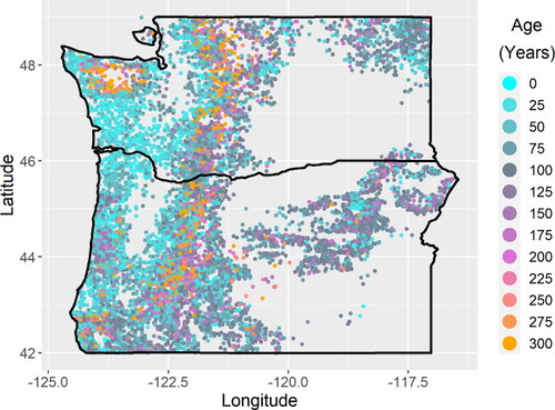
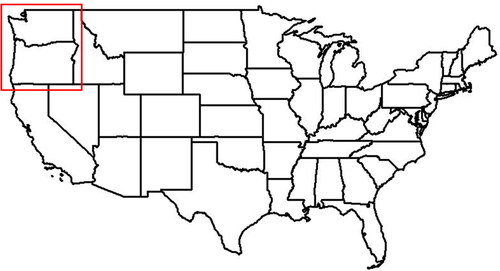
Tree-level carbon, board-foot volume, and species data and stand-level age data are obtained for an extensive set of surveyed forests from the Forest Inventory and Analysis (FIA) program from the US Forest Service [15,16]. Because western forests are sampled once per decade, sites surveyed during the last decade of the dataset are included over Washington and Oregon. We exclude sites that had experienced major mortality from a disturbance other than harvest since the last observation, because the inclusion of sites that have particularly young stand ages and carbon densities due to recent severe disturbance rather than timber harvest could cause us to overestimate the amount of additional carbon that could be sequestered by altering timber harvest practices. Carbon density is calculated as the carbon storage in aboveground live tree biomass in trees represented by FIA sampling (i.e. trees with at least a 5-inch diameter at breast height (d.b.h.)) per hectare for each site using tree-level data and information about subplot size.

Modeling

Growth parameters and variables are then empirically modeled across Washington and Oregon (Figure 1). While the coast, the Columbia River, and the western slope of the Cascades are the most intensively harvested subregions, we include interior subregions because of the existence of planted timber-producing forests even in less intensively harvested areas across the Pacific Northwest (see [14] for a recent map of planted timber-producing forests). For each site that contains live aboveground biomass, growth curves of the Gompertz form [17] are fitted for both aboveground live biomass carbon and board-foot volume as a function of stand age through a maximum likelihood approach using sites that are similar according to a combined metric of species composition and geographical distance (Text A1–A5, Figures A1–A7). No prior assumptions are made about growth based upon species composition or other characteristics (Text A1–A5). Plantation forestry in the Pacific Northwest is often conducted using even-aged regeneration, making growth and yield curves broadly appropriate for the most intensively harvested areas in this study [9, 17]. Nonetheless, because sites used for curve fitting are not able to be screened for single-aged stand structure and because multi-aged stands have a more complex relationship between canopy-class tree age and characteristics such as carbon density, wood volume, and diameter distribution [18–20], this empirical modeling approach using stand age may contribute to uncertainties. In addition, silvicultural treatments such as thinning, which are not explicitly accounted for in this analysis, also add variability in the relationship between canopy-class tree age and these growth characteristics and can be used to extend high growth rates [10, 19, 21]. Thus, although the combination of species composition and geography may implicitly account for other sources of variability such as management styles, the growth modeling in this study should be taken as a broad estimate, and it should be noted that growth trajectories may be altered through management. Despite these caveats, the model shows good agreement and no bias when used to predict the carbon density of FIA sites (Figures A2–A6).

Figure 1. The study area (Highlighted by a red square) comprises Washington and Oregon.

The age of CMAI is calculated using the wood volume growth curve for each applicable site. We assume that if stands are being harvested at the current age of CMAI on a cycle, then the median stand age over a large area of many stands of trees of a homogenous type under this management may converge to approximately half of the age of CMAI. We call one half of the CMAI age the optimal median stand age, and the associated expected carbon density the optimal median carbon density. This number should be taken as an approximation applicable only over a large area. This approximation would apply to an individual timber project only if that project were harvested in patches on a regular interval, a practice that does not reflect the reality of many timber projects.

To account for trunk diameter mill processing limitations in addition to limitations based on CMAI, we perform additional modeling following the same methods but for 95th percentile d.b.h. Sources familiar with the Pacific Northwest timber industry have cited 36 inches as a maximum diameter for demand and mill processing (e.g. D. Adams, personal communication, and [10]), so for sites at which the 95th percentile d.b.h. at the expected CMAI is expected to surpass this threshold, the optimal harvest age is decreased from CMAI to the age at which the 95th percentile d.b.h. equals 36 inches, rounded down to the nearest year. This threshold is somewhat arbitrary but provides an approximation of diameter limitations in the absence of publicly available data. A smaller diameter threshold based on typical demand, such as 24 inches [12] would further decrease the potential additional biomass carbon storage.

Carbon density deficit analysis

The observed and modeled characteristics are then translated into carbon density deficits. The median of each variable is gridded onto a 0.2 × 0.2° latitude–longitude grid (Text A5). On this grid, the optimal median stand age and carbon density for CMAI-limited and CMAI-and-diameter-limited rotation lengths are subtracted from the observed median stand age and carbon density in each grid cell. When calculating the median observed carbon density and stand age, sites with a stand age of zero and/or zero live aboveground biomass are included in order to capture recently cut patches that have not yet experienced enough regrowth to be included in the FIA tree survey. A bootstrap approach with 1000 iterations is used to quantify uncertainty bounds without prior knowledge of the probability distribution of carbon density deficits (Text A5). These deficits are expected to identify areas of widespread intensive harvest.

Finally, we estimate the total additional aboveground live biomass carbon that could be stored, averaged over the landscape and over harvest cycles, by extending rotation length, and we discuss this number in the context of the estimated implementation timescale from Fargione et al. [2] and relative to the magnitude of greenhouse gas emissions from this region. This number is expressed as the total additional carbon storage that would be reached under the new harvest schedule, not a per-year sequestration rate, because the additional carbon storage does saturate when the new harvest schedule is established. Exact locations and detailed ownership and harvest information are not publicly available for FIA plots, but ownership maps combined with the gridded forest data can identify areas of likely extensive harvest. Carbon density deficits are assumed to be representative of areas of particularly intensive and widespread timber harvest with relatively short rotation lengths, which in turn are associated with industrial forest ownership in the Pacific Northwest [22,23]. For this reason, carbon density deficits are assumed to be predominantly representative of forests owned by corporate entities and timber investment management organizations (TIMOs). Ownership maps are made available by the U.S. Forest Service [24]. For each grid cell with a carbon density deficit, that deficit is multiplied by the number of acres under corporate or TIMO ownership. If the surveyed forests of the grid cell include non-corporate, non-TIMO forests that systematically are older and more carbon-dense, then the corporate-owned forests would have an even greater carbon deficit than the grid cell average, resulting in an underestimation of the potential additional carbon. More generally, sub-grid cell heterogeneity in forest type and management would lead to uncertainties. However, this potential inaccuracy is unavoidable without specific ownership information or exact locations for individual sites.

Results and discussion

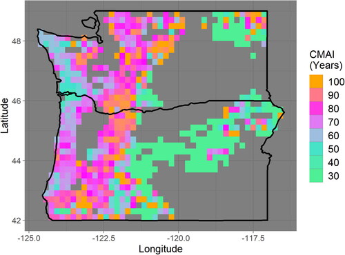
The CMAI is generally 50–70 years in heavily managed coastal regions (Figure 2). While large-scale variability across the entire Pacific Northwest landscape can clearly be attributed to the inclusion of forests that are not intensively managed across various topographies and climate conditions, other variability within intensively managed coastal regions appears associated with geography and species compositions. Areas near the delta of the Columbia River with a high proportion of western hemlock and western redcedar, two valuable timber species, appear to reach CMAI at 50 years or younger (Figures 2 and A1). Adjacent areas that are slightly more inland and dominated almost entirely by Douglas fir, a particularly common timber species, are shown here to reach CMAI at slightly older ages, such as 60 or 70 years, with CMAI generally increasing with distance from the coast (Figures 2 and S1). Both of these areas contain a large proportion of planted forests [14]. This analysis suggests that existing studies that assume a constant regional CMAI (e.g. Fargione et al. [2], which assumed a CMAI of 60 years across privately owned softwoods of this region) may be refined by accounting for smaller-scale variability in CMAI that may occur within intensively managed forests in the same region.

Figure 2. The modeled age at which stands are expected to reach the culmination of mean annual increment (CMAI) is gridded at a 0.2 × 0.2° latitude–longitude Resolution. This age varies widely across the Pacific Northwest. While small-scale variability likely represents noise, larger-scale patterns reveal regional characteristics. Please note that the color scale saturates at 30 and 100 years.

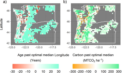
Despite relatively young ages of CMAI, opportunities to extend rotation length and increase average biomass carbon sequestration still exist, consistent with previous analyses [1,2]. A geographically coherent area from the central coast of Washington extending to the Colombia River on the border with Oregon shows the clearest pattern of a carbon deficit despite uncertainties of using these empirical methods with publicly available data. In this region, the estimated median stand age is more than 10 years younger than would be expected if consistently harvested at CMAI (Figure 3 panel a). This younger median age translates into a rotation length extension of more than 20 years (e.g. from 40 years to 60 years or more) and a carbon deficit of approximately100 − 200 metric tons of CO₂ storage per hectare in aboveground live biomass averaged over the landscape in this region, with much of this “deficit” being statistically significant at a 90% confidence level (Figure 3 panel b). Compared to the work of Fargione et al. [2], which assumes a rotation length extension from 40 or 45 years to a constant of 60 years across privately owned Pacific Northwest softwoods, this analysis finds an equal or even greater extension possible in many areas, but no extension possible in the area near the Columbia River delta. Despite the high rate of private ownership, planted forests, and valuable softwood timber species in the delta area, the extremely young age at which these forests reach CMAI precludes rotation length extensions, barring additional forest management strategies to prolong the period of rapid growth (Figures 2 and 3). When accounting for trunk diameter limitations associated with processing and industry demand, the magnitude of the deficit across western Washington marginally decreases, and a smaller area is statistically significant, but much of the area maintains a deficit on the same order of magnitude (Figure 4). This area of western Washington is the focus of the rest of the analysis.

Figure 3. Maps of the ages and aboveground live biomass carbon densities beyond optimal CMAI-constrained medians reveal large areas containing negative values, which indicate that the median age (panel (a)) and median carbon density (panel (b)) are less than what would be expected under a harvest schedule informed by CMAI. Approximately 9% of forested area grid cells contain such a carbon density deficit at 90% confidence, indicated by stippling. In western Washington and northwestern Oregon, these deficits are generally greater than 100 MTCO₂ ha⁻¹. The color scale saturates at a magnitude of 30 (panel (a)) and 300 (panel (b)).

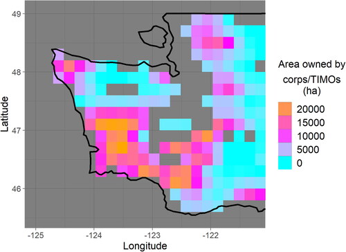
Integrating these carbon deficit estimates over corporate- and TIMO-owned forest area in western Washington (Figure 5), we find that when accounting for only CMAI-based limitations, approximately 100 million total additional metric tons of CO₂ (90% confidence interval: 19–260 MMt) is estimated to be able to be sequestered in aboveground live biomass averaged over the landscape and over harvest cycles. When CMAI and the diameter threshold are both accounted for, this estimate decreases to approximately 84 (3–240 90% CI) million metric tons. The larger uncertainty in the second case may result from the additional modeling that was necessary to assess trunk diameter growth. The confidence intervals span one to two orders of magnitude, highlighting the difficulties of using publicly available data to estimate potential additional carbon storage to a high degree of certainty. Further, additional uncertainties not captured by the bootstrap analysis may exist (Figure 5).

Figure 4. Data is displayed in the manner of Figure 2, panel (b), but optimal rotation length is defined by both CMAI and diameter threshold. The percent of grid cells in a carbon deficit at 90% confidence declines from approximately 9% to approximately 7%, with a particularly large loss of statistically significant deficit in western Washington. Some areas in western Washington completely lose a carbon deficit when diameter limitations are accounted for, while other simply decline in carbon deficit magnitude from nearly 200 to closer to 100 MTCO₂ ha⁻¹, with much of this remaining carbon deficit becoming statistically insignificant because of large uncertainties. As in Figure 2 panel (b), the color scale saturates at a magnitude of 300.

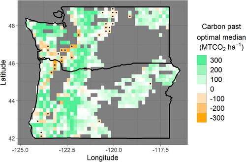
Figure 5. Eastern Washington contains large areas of forests owned by corporate entities and timber investment management operations (TIMOs). the total area in each 0.2 × 0.2° latitude–longitude grid cell at this latitude is approximately 35,000 ha.

The rate and magnitude of carbon sequestration and storage from improved forest management should be compared to that of gross emissions to understand the relative mitigation potential. The estimated additional sequestration potential in aboveground live biomass is approximately equal to one year of CO₂e emissions from Washington State [25]. However, the rotation length extension would take decades to centuries to implement, both because the rotation length extension itself is at a decadal scale and because this change in management would need to be implemented gradually over the landscape to avoid an abrupt short-term interruption in timber supply. Fargione et al. [2] estimate that extending all rotations in the Pacific Northwest to 60 years would take 150 to 200 years, assuming rotation extensions of 15 to 20 years implemented over 10 cohorts to limit reductions in timber harvest to 10%, a percentage that they find to be within the range of fluctuations in the timber supply. However, depending on market conditions, rotation extensions may need to be implemented even more gradually to avoid issues such as leakage and negative consequences for local employment. While a rotation extension may be able to be implemented more quickly if harvests increased on public lands with greater carbon densities to compensate for the temporarily reduced harvest from private lands [26], this method may prove controversial and incompatible with other environmental goals. More generally, if a temporary timber supply can be sourced elsewhere without becoming a source of long-term leakage, then rotation extensions may be implemented more quickly, but the logistics, local economic effects, and environmental implications may make this strategy unfeasible; an analysis of such a strategy is outside of the scope of this study.

Conclusion

Large-scale rotation extensions and increases in average biomass carbon storage are possible among heavily logged forests in the Pacific Northwest. However, it is important not to overstate the magnitude or rate of this additional carbon sequestration relative to gross greenhouse gas emissions, or the certainty of the exact amount of additional carbon able to be sequestered. Practical considerations greatly limit total additional sequestration and sequestration rates, leaving the realistic potential of additional carbon sequestration small relative to anthropogenic carbon emissions. In addition, the extent to which rotation length extensions are possible varies greatly within areas of intensively managed forests in this region.

Several factors not examined in this study are also relevant for the implementation of rotation extensions in planted forests in the Pacific Northwest. Carbon sequestration benefits through this improved forest management pathway may be exceeded by ecological and hydrological co-benefits [11, 27] and potential changes in industrial emissions associated with less frequent harvesting [28]. In addition, the potential for enhanced carbon sequestration through rotation extensions may be increased by management strategies such as thinning that can maintain high growth rates for longer periods of time [22]. Finally, challenges to implementation do exist. The temporary decrease in timber harvest that results from an increased rotation may have negative consequences for supply chains and local employment [11]. The mechanisms that may be used to incentivize rotation lengths should also be examined for their economic effects. For example, the sale of carbon offsets could incentivize longer rotation ages for enrolled land owners, but questions of harvest decrease and leakage incentivized by such programs, as well as the distribution of economic benefits from carbon payments, should be considered [29].

Acknowledgments

Dr. Darius Adams (Professor Emeritus, Oregon State University), Dr. Brian Buma (Senior Climate Scientist, Environmental Defense Fund), Dr. Steven Hamburg (Chief Scientist, Environmental Defense Fund), and Mr. Eric Holst (Vice President of Natural Climate Solutions, Environmental Defense Fund) provided feedback on the scientific merit and policy relevance of this manuscript.

Disclosure statement

No potential conflict of interest was reported by the authors.

Data availability statement

All tree level, plot level, and condition level Forest Inventory and Analysis (FIA) data used in this analysis can be found at the FIA DataMart at https://apps.fs.usda.gov/fia/datamart/datamart.html courtesy of the United States Forest Service (USFS).

The forest ownership data used in this analysis can be found at the USFS Research Data Archive at https://www.fs.usda.gov/rds/archive/Catalog/RDS-2020-0044.

Additional information

Funding

This work was funded by an award from Earth Fund to Environmental Defense Fund.

Appendix

Text A1: Overview of modeling

Modeling is carried out for each individual site with nonzero aboveground biomass. Aboveground live biomass and board-foot volume are both modeled. The board-foot volume modeling is used to calculate the mean annual increment (MAI) of timber in order to determine the biological optimum age of timber harvest. The aboveground live biomass modeling is used to estimate on-site carbon storage across the harvest rotation in this carbon pool.

Modeling site-by-site using this method, rather than fitting a single growth curve for each grid cell using the sites contained within the grid cell, allows the number of sites used for each fitting to be greater than the number of sites located in each grid cell. This method also allows for heterogeneity in growth parameters (and therefore in CMAI and related variables) to exist within each grid cell, which in turn provides one computationally inexpensive way to estimate uncertainties via bootstrap resampling (described later).

Text A2: Identification of similar sites to use for growth curve fitting

For each site, the sites used in its growth curve fitting are identified using a combined metric of species composition and geographical distance.

To create species composition variables, a principal component analysis (PCA) is performed on species percentage by basal area over all sites that contain live trees (Figure A1). The procedure follows that of Randazzo et al. [30]. The first four PCA axes, representing approximately 16% of all species composition variability, are used to determine proximity between sites in species composition space. The importance of each axis is weighted by the associated eigenvalue.

The geographical distance variable is constructed using simple spatial distances between sites. While site locations are nudged by approximately 800 meters and are therefore not exact, and while some site locations are swapped with similar nearby sites, the inclusion of even this approximate geographical distance metric lessens geographical biases in the empirical growth model (The geographical distribution of residuals can be seen in Figure A6). Both of these distance metrics are normalized and combined into a single metric. 0.5% of all sites with live aboveground biomass in this region (or 52 sites out of 10305 sites) are used for each fitting.

Text A3: Growth curve form

The Gompertz curve takes the form $k{e}^{{-e}^{a-bt}},$ where t is time (in this case, stand age). The parameter k is the carrying capacity, or the level to which the asymptote is set. The parameters a and b together control the growth rate and inflection point. For biomass carbon and timber volume modeling, it is enforced that the value must equal zero at time zero. For trunk diameter modeling, a positive intercept is allowed, in order to account for discontinuity.

Text A4: Maximum likelihood parameter optimization

For each site, the parameters were fitted using a maximum likelihood approach by iteratively minimizing a cost function. The derivation of the cost function begins with a function proportional to the negative logarithm of either a normal or skew-normal distribution. The decision to use either a normal or skew-normal distribution in the derivation of this function is made automatically by the program for each iteration depending on whether the skewness of residuals on that iteration is greater than or less than 1. Let x denote the residual vector. Then, assuming a normal distribution of uncorrelated residuals with constant variance, the negative logarithm of the likelihood function is proportional to x^Tx, or the sum of squared residuals (the superscript “T” designates the transpose of a vector or matrix). Making the same variance-covariance assumptions but assuming a skew-normal distribution, the cost function is then x^Tx+y^Ty, where y is a vector of the cumulative sum of ordered residuals. However, the variance of residuals increases with the stand age of the forest (Figure S4). This increasing variance is modeled as variance being proportional to $\frac{t+1}{t+25},$ where t is the stand age. If C denotes a variance-covariance matrix with this variance proportion on the diagonal and zeros off the diagonal (under the assumption of no significant covariance between residuals), then the expression x^TCx is proportional to the negative logarithm of the likelihood function. For the skew-normal case, this becomes x^TCx+y^TC₁y, where the diagonal entries of C₁ are ordered to correspond to the ordered residuals in y. This expression then can be used as the cost function to be iteratively minimized to optimize the growth parameters.

Text A5: Gridding and bootstrapping uncertainty bounds

The observed carbon density, observed stand age, optimal median carbon density, and optimal median stand age are gridded onto a 0.2 × 0.2° latitude–longitude grid. The grid cell values represent the median of these variables over all sites within the grid cell. The optimal median carbon density is subtracted from the observed median carbon density for each grid cell. Negative values indicate that a grid cell contains forests with a lower median carbon density than would be expected under a rotation length of CMAI, or in a “carbon deficit.” Only grid cells containing at least 5 observations (an arbitrary threshold) are included.

Within each 0.2 × 0.2° latitude–longitude grid cell, individual sites are sampled 1000 times, allowing repeats. Median optimum carbon density and age are found in each grid cell for each iteration, as are the median optimum carbon density and age. For each iteration, gridded optimal median carbon density is subtracted from gridded median observed carbon density to obtain a gridded carbon density deficit. The 5th and 95th percentiles of this gridded carbon density deficit then represent the bounds of a 90% confidence interval. These uncertainty bounds are then used to calculate uncertainty bounds of the potential additional carbon sequestration across corporate and TIMO forest areas. Furthermore, for any given grid cell, carbon deficit is significant at the 90% confidence level when the 90th percentile of (observed median carbon density – optimal median carbon density) is negative.

Figure A1. (a) FIA sites with nonzero live tree biomass are projected onto the first two PCA axes, which together account for 8.7% of variability across 10,305 sites. Species associated with the most variability are (clockwise from upper left) WR (western redcedar), WH (western hemlock), PSF (Pacific silver fir), MH (Mountain hemlock), SF (subalpine fir), ES (Engelmann spruce), LP (lodgepole pine), PP (ponderosa pine), PM (Pacific madrone), and DF (Douglas fir). (b) In coastal areas, most forests are associated with the presence of Douglas fir, western hemlock, and/or western redcedar.

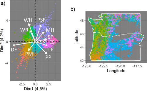
Figure A2. When fitted growth parameters for each site are used to reproduce the aboveground live tree carbon of the corresponding site, the aggregated residuals are centered at zero, slightly skewed, and highly peaked. While the residuals for each parameter fitting for each individual site are assumed either normal or skew-normal (i.e. having a smaller peak than is seen here), a greater number of fittings that produce lower variance and a smaller number of fittings that produce a higher variance would produce this high peak when all residuals are aggregated. Fittings all allow for skew in the residuals (a characteristic that may be preserved in residual aggregation if skew occurs more often in one direction) and assume unbiasedness of the model (a characteristic that would be preserved during residual aggregation), so these characteristics of the aggregated residuals distribution are also consistent with the prior assumptions used in model fitting. The width of the bins in this histogram is 10 MT CO₂ ha⁻¹. A white vertical line overlaying the histogram designates zero.

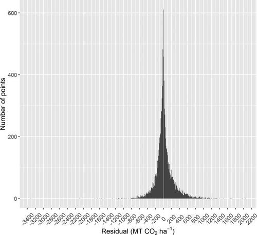
Figure A3. Modeled versus observed aboveground live tree carbon approximately follow the 1:1 line (denoted in white).

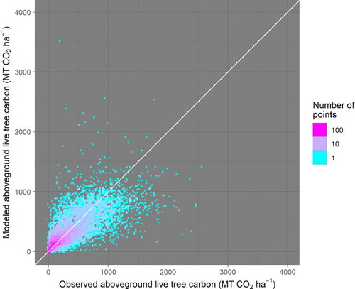
Figure A4. Aggregated residuals are unbiased by stand age. They do, however, display an increased variance with increased stand age, and this phenomenon is accounted for in the prior assumptions used in model fitting (Text A1.3). Please note that one datapoint is eliminated from this figure because of a reported stand age of 10,000 years.

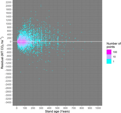
Figure A5. The residuals do not show a correlation with modeled carbon. The variance of residuals does increase with modeled carbon, a phenomenon related to increasing variance with stand age, which is accounted for in the model fitting (Text A1–A4). Because all values are bounded at zero (i.e. carbon stocks cannot be negative), residuals are bounded at the −1:1 line.

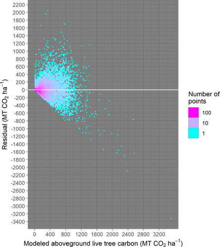
Figure A6. The geographic distribution of residuals for all sites with recorded live trees shows no clear geographical biases. The magnitude of residuals, however, does vary with geography, but this phenomenon can be explained by the variation of average stand age with geography (Figure A7). the relationship between residual magnitude and stand age is accounted for in the model fitting (Text A1–A4).

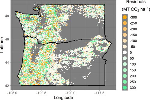
Figure A7. the geographical differences in stand age can explain the geographical differences in residual magnitude seen in Figure A6.

References

- Griscom BW, Adams J, Ellis PW, et al. Natural climate solutions. Proc Natl Acad Sci U S A. 2017;114(44):11645–11650. doi: 10.1073/pnas.1710465114.
- Fargione JE, Bassett S, Boucher T, et al. Natural climate solutions for the United States. Sci Adv. 2018;4(11):eaat1869. doi: 10.1126/sciadv.aat1869.
- Law BE, Hudiburg TW, Berner LT, et al. Land use strategies to mitigate climate change in carbon dense temperate forests. Proc Natl Acad Sci U S A. 2018;115(14):3663–3668. doi: 10.1073/pnas.1720064115.
- Zuckerman S. Longer rotations and carbon. Northwest Natural Resource Group, Dec 08, 2021. [cited 2023 Feb 16]. Available from: https://www.nnrg.org/longer-rotations-and-carbon.
- Anderson K. Yes, long rotations can yield real climate gains for Cascadia. Sightline Institute, Mar. 17, 2022. [cited 2022 Aug 15]. Available from: https://www.sightline.org/2022/03/17/yes-long-rotations-can-yield-real-climate-gains-for-cascadia/.
- Stokland JN. Volume increment and carbon dynamics in boreal Forest when extending the rotation length towards biologically old stands. For Ecol Manage. 2021;488:119017. doi: 10.1016/j.foreco.2021.119017.
- Petersson H, Ellison D, Appiah Mensah A, et al. “On the role of forests and the Forest sector for climate change mitigation in Sweden. GCB Bioenergy. 2022;14(7):793–813. doi: 10.1111/gcbb.12943.
- Kaipainen T, Liski J, Pussinen A, et al. Managing carbon sinks by changing rotation length in european forests. Environ Sci Policy. 2004;7(3):205–219. Jun. doi: 10.1016/j.envsci.2004.03.001.
- Ashton MS, Kelty MJ. Tree and stand growth. In The practice of silviculture: applied forest ecology. 10th ed. Hoboken, NY: John Wiley & Sons Ltd., 2018.
- Hall ES. Thoughts on the longer rotation climate solution for Washington state – Is it a sure bet? Three Trees Consulting, Mar. 19, 2022. [cited 2023 Feb 14]. Available from: https://www.threetreesforestry.com/post/thoughts-on-the-longer-rotation-climate-solution-for-washington-state-is-it-a-sure-bet.
- Roberge J-M, Laudon H, Björkman C, et al. Socio-ecological implications of modifying rotation lengths in forestry. Ambio. 2016;45(Suppl. 2):109–123. doi: 10.1007/s13280-015-0747-4.
- Haynes R. Will markets provide sufficient incentive for sustainable forest management?. Pacific Northwest Research Station, US Forest Service, 2005. [cited 2023 Feb 27]. Available from: https://www.fs.usda.gov/pnw/publications/understanding-key-issues-sustainable-wood-production-pacific-northwest.
- FoleyTG, Richter D D, Galik CS. Extending rotation age for carbon sequestration: a cross-protocol comparison of North American Forest offsets. For Ecol Manage. 2009;259(2):201–209. doi: 10.1016/j.foreco.2009.10.014.
- Perry CH, Finco MV, Wilson BT. Forest atlas of the United States. U.S. Department of Agriculture. 2022; Forest Service, Washington, DC, FS-1172, Jun. doi: 10.2737/FS-1172.
- Burrill EA, et al. The Forest inventory and analysis database: database description and user guide for phase 2 (version 8.0). 2018.
- Forest Inventory and Analysis Database, 2023. [cited 2023 Mar 17]. Available from: https://apps.fs.usda.gov/fia/datamart/datamart.html.
- Winsor CP. The Gompertz curve as a growth curve. Proc Natl Acad Sci U S A. 1932;18(1):1–8. doi: 10.1073/pnas.18.1.1.
- Harper G, Omari K, Kranabetter M, et al. Assessment of a 20-year-old mixed Western redcedar/red alder plantation in southwestern British Columbia. For Ecol Manage. 2023;529:120737. Feb. doi: 10.1016/j.foreco.2022.120737.
- Bowman DMJS, Brienen RJW, Gloor E, et al. Detecting trends in tree growth: not so simple. Trends Plant Sci. 2013;18(1):11–17. Jan doi: 10.1016/j.tplants.2012.08.005.
- Harrington TB, Peter DH, Marshall DD, et al. Ten-year Douglas-fir regeneration and stand productivity differ among contrasting silvicultural regimes in Western Washington, USA. For Ecol Manage. 2022;510:120102. Apr. doi: 10.1016/j.foreco.2022.120102.
- Peng C. Growth and yield models for uneven-aged stands: past, present and future. For Ecol Manage. 2000;132(2-3):259–279. Jul doi: 10.1016/S0378-1127(99)00229-7.
- Tappeiner J, Adams D, Montgomery C, et al. Growth of managed older Douglas-fir stands: implications of the black rock thinning trial in the Coast range of Western Oregon. J Forestry. 2022;120(3):282–288. doi: 10.1093/jofore/fvab063.
- Masek JG, Cohen WB, Leckie D, et al. Recent rates of Forest harvest and conversion in North America. J. Geophys. Res. 2011;116(G4):G00K03. doi: 10.1029/2010JG001471.
- Sass EM, Butler BJ, Markowski-Lindsay MA. Forest ownership in the conterminous United States circa 2017: distribution of eight ownership types – geospatial dataset. 2020. doi: 10.2737/RDS-2020-0044.
- Washington State Department of Ecology. GHG inventories. [cited 2023 Jan 27]. Available from: https://ecology.wa.gov/Air-Climate/Reducing-Emissions/Tracking-greenhouse-gases/GHG-inventories.
- Im EH, Adams DM, Latta GS. The impacts of changes in federal timber harvest on Forest carbon sequestration in Western Oregon. Can. J. For. Res. 2010;40(9):1710–1723. doi: 10.1139/X10-110.
- Curtis RO, Carey AB. Timber supply in the pacific northwest: managing for economic and ecological values in douglas-fir Forest. J Forestry. 1996;94(9):4–7. Available from: https://www.srs.fs.usda.gov/pubs/6163
- Gunn JS, Buchholz T. Forest sector greenhouse gas emissions sensitivity to changes in Forest management in Maine (USA). Forestry. 2018;91(4):526–538. doi: 10.1093/forestry/cpy013.
- Latta GS, Adams DM, Bell KP, et al. Evaluating land-use and private Forest management responses to a potential Forest carbon offset sales program in Western Oregon (USA). Forest Policy Econ. 2016;65:1–8. doi: 10.1016/j.forpol.2016.01.004.
- Randazzo NA,Gordon DR,Hamburg SP. Improved assessment of baseline and additionality for Forest carbon crediting. Ecol Appl. 2023;33(3):e2817. doi:10.1002/eap.2817.