A tutorial introduction to reinforcement learning

Abstract

In this paper, we present a brief survey of reinforcement learning, with particular emphasis on stochastic approximation (SA) as a unifying theme. The scope of the paper includes Markov reward processes, Markov decision processes, SA algorithms, and widely used algorithms such as temporal difference learning and Q-learning.

Keywords:

• Markov decision processes
• Bellman optimality
• value iteration
• Q-iteration
• stochastic approximation

1. Introduction

In this paper, we present a brief survey of reinforcement learning (RL), with particular emphasis on stochastic approximation (SA) as a unifying theme. The scope of the paper includes Markov reward processes, Markov decision processes (MDPs), SA methods, and widely used algorithms such as temporal difference learning and Q-learning. RL is a vast subject, and this brief survey can barely do justice to the topic. There are several excellent texts on RL, such as Refs. [1–4]. The dynamics of the SA algorithm are analysed in Refs. [5–11]. The interested reader may consult those sources for more information.

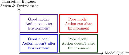
In this survey, we use the phrase “ RL” to refer to decision-making with uncertain models, and in addition, current actions alter the future behaviour of the system. Therefore, if the same action is taken at a future time, the consequences might not be the same. This additional feature distinguishes RL from “mere” decision-making under uncertainty. Figure 1 rather arbitrarily divides decision-making problems into four quadrants. Examples from each quadrant are now briefly described.

• Many if not most decision-making problems fall into the lower-left quadrant of “good model, no alteration” (meaning that the control actions do not alter the environment). An example is a fighter aircraft which usually has an excellent model, thanks to aerodynamical modelling and/or wind tunnel tests. In turn this permits the control system designers to formulate and to solve an optimal (or some other form of) control problem.

• Controlling a chemical reactor would be an example from the lower-right quadrant. As a traditional control system, it can be assumed that the environment in which the reactor operates does not change as a consequence of the control strategy adopted. However, due to the complexity of a reactor, it is difficult to obtain a very accurate model, in contrast with a fighter aircraft for example. In such a case, one can adopt one of two approaches. The first, which is a traditional approach in control system theory, is to use a nominal model of the system and to treat the deviations from the nominal model as uncertainties in the model. A controller is designed based on the nominal model, and robust control theory would be invoked to ensure that the controller would still perform satisfactorily (though not necessarily optimally) for the actual system. The second, which would move the problem from the lower right to the upper-right quadrant, is to attempt to “learn” the unknown dynamical model by probing its response to various inputs. This approach is suggested in Ref. [4, Example 3.1]. A similar statement can be made about robots, where the geometry determines the form of the dynamical equations describing it, but not the parameters in the equations; see, for example, Ref. [12]. In this case too, it is possible to “learn” the dynamics through experimentation. In practice, such an approach is far slower than the traditional control systems approach of using a nominal model and designing a “robust” controller. However, “learning control” is a popular area in the world of machine learning. One reason is that the initial modelling error is too large, then robust control theory alone would not be sufficient to ensure the stability of the actual system with the designed controller. In contrast (and in principle), a “learning control” approach can withstand larger modelling errors. The widely used model predictive control paradigm can be viewed as an example of a learning-based approach.

• A classic example of a problem belonging to the upper-left corner is a MDP, which forms the backbone of one approach to RL. In an MDP, there is a state space $\mathcal{X}$ and an action space $\mathcal{U}$, both of which are usually assumed to be finite. In most MDPs, $|\mathcal{X}|\gg |\mathcal{U}|$. Board games without an element of randomness such as tic-tac-toe or chess would belong to the upper-left quadrant, at least in principle. Tic-tac-toe belongs here, because the rules of the game are clear, and the number of possible games is manageable. In principle, games such as chess which are “deterministic” (i.e. there is no throwing of dice as in Backgammon for example) would also belong here. Chess is a two-person game in which, for each board position, it is possible to assign the likelihood of the three possible outcomes: white wins, black wins, or it is a draw. However, due to the enormous number of possibilities, it is often not possible to determine these likelihoods precisely. It is pointed out explicitly in Ref. [13] that merely because we cannot explicitly compute this likelihood function, that does not mean that the likelihood does not exist! However, as a practical matter, it is not a bad idea to treat this likelihood function as being unknown, and to infer it on the basis of experiment/experience. Thus, as with chemical reactors, it is not uncommon to move chess-playing from the lower-right corner to the upper-right corner.

• The upper-right quadrant is the focus of RL. There are many possible ways to formulate RL problems, each of which leads to its own solution methodologies. A very popular approach to RL is to formulate it as MDPs whose dynamics are unknown. That is the approach adopted in this paper.

Figure 1. The four quadrants of decision-making under uncertainty.

In an MDP, at each time t, the learner (also known as the actor or the agent) measures the state $X_t\in \mathcal{X}$. Based on this measurement, the learner chooses an action $U_t\in \mathcal{U}$ and receives a reward $R(X_t,U_t)$. Future rewards are discounted by a discount factor $\gamma \in (0,1)$. The rule by which the current action $U_t$ is chosen as a function of the current state $X_t$ is known as a policy. With each policy, one can associate the expected value of the total (discounted) reward over time. The problem is to find the best policy. There is a variant called partially observable MDP in which the state $X_t$ cannot be measured directly; rather, there is an output (or observation) $Y_t\in \mathcal{Y}$ which is a memoryless function, either deterministic or random, of $X_t$. 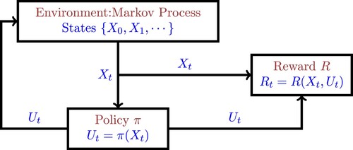These problems are not studied here; it is always assumed that $X_t$ can be measured directly. When the parameters of the MDP are known, there are several approaches to determining the optimal policy. RL is distinct from an MDP in that, in RL, the parameters of the underlying MDP are constant but not known to the learner; they must be learnt on the basis of experimentation. Figure 2 depicts the situation.

Figure 2. Depiction of a RL problem.

The remainder of the paper is organized as follows: in Section 2, Markov reward processes are introduced. These are a precursor to MDPs, which are introduced in Section 3. Specifically, in Section 3.1, the relevant problems in the study of MDPs are formulated. In Section 3.2, the solutions to these problems are given in terms of the Bellman value iteration, the action-value function, and the F-iteration to determine the optimal action-value function. In Section 3.3, we study the situation where the dynamics of the MDP under study are not known precisely. Instead, one has access only to a sample path $\left\{X_t\right\}$ of the Markov process under study. For this situation, we present two standard algorithms, known as temporal difference learning and Q -learning. Starting from Section 4, the paper consists of results due to the author. In Section 4.1, the concept of SA is introduced, and its relevance to RL is outlined in Section 4.2. In Section 4.3, a new theorem on the global asymptotic stability of nonlinear ODEs is stated; this theorem is of independent interest. Some theorems on the convergence of the SA algorithm are presented in Sections 4.4 and 4.5. In Section 5, the results of Section 4 are applied to RL problems. In Section 5.1, a technical result on the sample paths of an irreducible Markov process is stated. Using this result, simplified conditions are given for the convergence of the temporal difference algorithm (Section 5.2) and Q-learning (Section 5.3). A brief set of concluding remarks ends the paper.

2. Markov reward processes

Markov reward processes are standard (stationary) Markov processes where each state has a “reward” associated with it. Markov reward processes are a precursor to MDPs; so we review those in this section. There are several standard texts on Markov processes, one of which is Ref. [14].

Suppose $\mathcal{X}$ is a finite set of cardinality n, written as $\{x_1,\dots ,x_n\}$. If $\{X_t{\}}_{t\ge 0}$ is a stationary Markov process assuming values in $\mathcal{X}$, then the corresponding state transition matrix A is defined by (1) $\begin{array}{r}{a}_{ij}=Pr\{X_{t+1}=x_j|X_t=x_i\}.\end{array}$(1) Thus the ith row of A is the conditional probability vector of $X_{t+1}$ when $X_t=x_i$. Clearly the row sums of the matrix A are all equal to one. This can be expressed as $A{\mathbf{1}}_n={\mathbf{1}}_n$, where ${\mathbf{1}}_n$ denotes the n-dimensional column vector whose entries all equal to one. Therefore, if we define the induced matrix norm $\Vert A{\Vert }_{\mathrm{\infty }\to \mathrm{\infty }}$ as $\Vert A{\Vert }_{\mathrm{\infty }\to \mathrm{\infty }}:=\underset{\mathbf{v}\ne \mathbf{0}}{max}\frac{\Vert A\mathbf{v}{\Vert }_{\mathrm{\infty }}}{\Vert \mathbf{v}{\Vert }_{\mathrm{\infty }}},$then $\Vert A{\Vert }_{\mathrm{\infty }\to \mathrm{\infty }}$ equals one, which also equals the spectral radius of A.

Now suppose that there is a “reward” function $R:\mathcal{X}\to \mathbb{R}$ associated with each state. There is no consensus within the community about whether the reward corresponding to the state $X_t$ is paid at time t as in Ref. [3] or time t + 1 as in Refs. [2,4]. In this paper, it is assumed that the reward is paid at time t and is denoted by $R_t$; the modifications required to handle the other approach are easy and left to the reader. The reward $R_t$ can either be a deterministic function of $X_t$ or a random function. If $R_t$ is a deterministic function of $X_t$, then we have that $R_t=R\left(X_t\right)$ where R is the reward function mapping $\mathcal{X}$ into (a finite subset of) $\mathbb{R}$. Thus, whenever the trajectory $\left\{X_t\right\}$ of the Markov process equals some state $x_i\in \mathcal{X}$, the resulting reward $R\left(X_t\right)$ will always equal $R\left(x_i\right)=:r_i$. Thus the reward is captured by an n-dimensional vector $\mathbf{r}$, where $r_i=R\left(x_i\right)$. On the other hand, if $R_t$ is a random function of $X_t$, then one would have to provide the probability distribution of $R_t$ given $X_t$. Since $X_t$ has only n different values, we would have to provide n different probability distributions. To avoid technical difficulties, it is common to assume that $R\left(x_i\right)$ is a bounded random variable for each index i. Note that because the set $\mathcal{X}$ is finite, if the reward function is deterministic, then we have that $\underset{x_i\in \mathcal{X}}{max}R\left(x_i\right)<\mathrm{\infty }.$In case the reward function R is random, as mentioned above, it is common to assume that $R\left(x_i\right)$ is a bounded random variable for each index $i\in \left[n\right]$, where the symbol $\left[n\right]$ equals $\{1,\dots ,n\}$. With this assumption, it follows that $\underset{x_i\in \mathcal{X}}{max}E\left[R\right(x_i\left)\right]<\mathrm{\infty }.$Two kinds of Markov reward processes are widely studied, namely: discounted reward processes and average reward processes. In this paper, we restrict attention to discounted reward processes. However, we briefly introduce average reward processes. Define (if it exists) $V\left(x_i\right):=\underset{T\to 0}{lim}\frac{1}{T+1}E\left[\sum _{t=0}^{T}R\right(X_t)|X_0=x_i].$An excellent review of average reward processes can be found in Ref. [15].

In each discounted Markov reward process, there is a “discount factor” $\gamma \in (0,1)$. This factor captures the extent to which future rewards are less valuable than immediate rewards. Fix an initial state $x_i\in \mathcal{X}$. Then the expected discounted future reward $V\left(x_i\right)$ is defined as (2) $\begin{array}{rl}V\left(x_i\right)& :=E[\sum _{t=0}^{\mathrm{\infty }}{\gamma }^t{R}_t|X_0=x_i]\\ & =E\left[\sum _{t=0}^{\mathrm{\infty }}{\gamma }^{t}R\right(X_t)|X_0=x_i].\end{array}$(2) We often just use “discounted reward” instead of the longer phrase. With these assumptions, because $\gamma <1$, the above summation converges and is well defined. The quantity $V\left(x_i\right)$ is referred to as the value function associated with $x_i$, and the vector (3) $\begin{array}{r}\mathbf{v}=[\begin{array}{lll}V\left(x_1\right)& \cdots & V\left(x_n\right)\end{array}{]}^{\mathrm{\top }}\end{array}$(3) is referred to as the value vector. Note that, throughout this paper, we view the value as both a function $V:\mathcal{X}\to \mathbb{R}$ as well as a vector $\mathbf{v}\in {\mathbb{R}}^n$. The relationship between the two is given by (3(3) $\begin{array}{r}\mathbf{v}=[\begin{array}{lll}V\left(x_1\right)& \cdots & V\left(x_n\right)\end{array}{]}^{\mathrm{\top }}\end{array}$(3) ). We shall use whichever interpretation is more convenient in a given context.

This raises the question as to how the value function and/or value vector is to be determined. Define the vector $\mathbf{r}\in {\mathbb{R}}^n$ via (4) $\begin{array}{r}\mathbf{r}:=[\begin{array}{lll}{r}_1& \cdots & r_n\end{array}{]}^{\mathrm{\top }},\end{array}$(4) where $r_i=R\left(x_i\right)$ if R is a deterministic function, and if $R_t$ is a random function of $X_t$, then (5) $\begin{array}{r}{r}_i:=E\left[R\right(x_i\left)\right].\end{array}$(5) The next result gives a useful characterization of the value vector.

Theorem 2.1

The vector $\mathbf{v}$ satisfies the recursive relationship (6) $\begin{array}{r}\mathbf{v}=\mathbf{r}+\gamma A\mathbf{v},\end{array}$(6) or, in expanded form, (7) $\begin{array}{r}V\left(x_i\right)=r_i+\gamma \sum _{j=1}^n{a}_{ij}V\left(x_j\right).\end{array}$(7)

Proof.

Let $x_i\in \mathcal{X}$ be arbitrary. Then by definition we have (8) $\begin{array}{rl}V\left(x_i\right)& =E[\sum _{t=0}^{\mathrm{\infty }}{\gamma }^t{R}_t|X_0=x_i]\\ & =r_i+E[\sum _{t=1}^{\mathrm{\infty }}{\gamma }^t{R}_t|X_0=x_i].\end{array}$(8) However, if $X_0=x_i$, then $X_1=x_j$ with probability $a_{ij}$. Therefore, we can write (9) $\begin{array}{rl}& E[\sum _{t=1}^{\mathrm{\infty }}{\gamma }^t{R}_t|X_0=x_i]\\ & =\sum _{j=1}^n{a}_{ij}E[\sum _{t=1}^{\mathrm{\infty }}{\gamma }^t{R}_t|X_1=x_j]\\ & =\gamma \sum _{j=1}^n{a}_{ij}E[\sum _{t=0}^{\mathrm{\infty }}{\gamma }^t{R}_t|X_0=x_j]\\ & =\gamma \sum _{j=1}^n{a}_{ij}V\left(x_j\right).\end{array}$(9) In the second step we use the fact that the Markov process is stationary. Substituting  (9(9) $\begin{array}{rl}& E[\sum _{t=1}^{\mathrm{\infty }}{\gamma }^t{R}_t|X_0=x_i]\\ & =\sum _{j=1}^n{a}_{ij}E[\sum _{t=1}^{\mathrm{\infty }}{\gamma }^t{R}_t|X_1=x_j]\\ & =\gamma \sum _{j=1}^n{a}_{ij}E[\sum _{t=0}^{\mathrm{\infty }}{\gamma }^t{R}_t|X_0=x_j]\\ & =\gamma \sum _{j=1}^n{a}_{ij}V\left(x_j\right).\end{array}$(9) ) into (8(8) $\begin{array}{rl}V\left(x_i\right)& =E[\sum _{t=0}^{\mathrm{\infty }}{\gamma }^t{R}_t|X_0=x_i]\\ & =r_i+E[\sum _{t=1}^{\mathrm{\infty }}{\gamma }^t{R}_t|X_0=x_i].\end{array}$(8) ) gives the recursive relationship (7(7) $\begin{array}{r}V\left(x_i\right)=r_i+\gamma \sum _{j=1}^n{a}_{ij}V\left(x_j\right).\end{array}$(7) ).

Example 2.2

As an illustration of a Markov reward process, we analyse a toy snakes and ladders game with the transitions shown in Figure 3. Here W and L denote “win” and “lose,” respectively. The rules of the game are as follows:

• Initial state is S.

• A four-sided, fair die is thrown at each stage.

• Player must land exactly on W to win and exactly on L to lose.

• If implementing a move causes crossing of W and L, then the move is not implemented.

Figure 3. A toy snakes and ladders game.

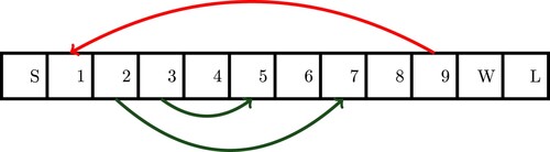
There are 12 possible states in all: S, 1, …, 9, W, and L. However, 2, 3, and 9 can be omitted, leaving nine states, namely S, 1, 4, 5, 6, 7, 8, W, and L. At each step, there are at most four possible outcomes. For example, from the state S, the four outcomes are 1, 7, 5, and 4. From state 6, the four outcomes are 7, 8, 1, and W. From state 7, the four outcomes are 8, 1, W, and 7. From state 8, there four possible outcomes are 1, W, L, and 8 with probability 1/4 each, because if the die comes up with 4, then the move cannot be implemented. It is time-consuming but straight-forward to compute the state transition matrix as $\begin{array}{|cccccccccc|}\hline & S& 1& 4& 5& 6& 7& 8& W& L\\ S& 0& 0.25& 0.25& 0.25& 0& 0.25& 0& 0& 0\\ 1& 0& 0& 0.25& 0.50& 0& 0.25& 0& 0& 0\\ 4& 0& 0& 0& 0.25& 0.25& 0.25& 0.25& 0& 0\\ 5& 0& 0.25& 0& 0& 0.25& 0.25& 0.25& 0& 0\\ 6& 0& 0.25& 0& 0& 0& 0.25& 0.25& 0.25& 0\\ 7& 0& 0.25& 0& 0& 0& 0& 0.25& 0.25& 0.25\\ 8& 0& 0.25& 0& 0& 0& 0& 0.25& 0.25& 0.25\\ W& 0& 0& 0& 0& 0& 0& 0& 1& 0\\ L& 0& 0& 0& 0& 0& 0& 0& 0& 1\\ \hline\end{array}$

We define a reward function for this problem as follows: we set $R_t=f\left(X_{t+1}\right)$, where f is defined as follows: $f\left(W\right)=5$, $f\left(L\right)=-2$, and $f\left(x\right)=0$ for all other states. However, there is an expected reward depending on the state at the next time instant. For example, if $X_0=6$, then the expected value of $R_0$ is 5/4, whereas if $X_0=7$ or $X_0=8$, then the expected value of $R_0$ is 3/4.

Now let us see how the implicit equation (6(6) $\begin{array}{r}\mathbf{v}=\mathbf{r}+\gamma A\mathbf{v},\end{array}$(6) ) can be solved to determine the value vector $\mathbf{v}$. Since the induced matrix norm $\Vert A{\Vert }_{\mathrm{\infty }\to \mathrm{\infty }}=1$ and $\gamma <1$, it follows that the matrix $I-\gamma A$ is nonsingular. Therefore, for every reward function $\mathbf{r}$, there is a unique $\mathbf{v}$ that satisfies (6(6) $\begin{array}{r}\mathbf{v}=\mathbf{r}+\gamma A\mathbf{v},\end{array}$(6) ). In principle, it is possible to deduce from (6(6) $\begin{array}{r}\mathbf{v}=\mathbf{r}+\gamma A\mathbf{v},\end{array}$(6) ) that (10) $\begin{array}{r}\mathbf{v}=(I-\gamma A{)}^{-1}\mathbf{r}.\end{array}$(10) The difficulty with this formula however is that in most actual applications of Markov decision problems, the integer n denoting the size of the state space $\mathcal{X}$ is quite large. Moreover, inverting a matrix has cubic complexity in the size of the matrix. Therefore, it may not be practicable to invert the matrix $I-\gamma A$. So we are forced to look for alternate approaches. A feasible approach is provided by the contraction mapping theorem.

Theorem 2.3

The map $\mathbf{y}\mapsto T\mathbf{y}:=\mathbf{r}+\gamma A\mathbf{y}$ is monotone and is a contraction with respect to the ${\ell }_{\mathrm{\infty }}$-norm, with contraction constant γ. Therefore, we can choose some vector ${\mathbf{y}}^0$ arbitrarily, and then define ${\mathbf{y}}^{i+1}=\mathbf{r}+\gamma A{\mathbf{y}}^i.$Then ${\mathbf{y}}^i$ converges to the value vector $\mathbf{v}$.

Proof.

The first statement is that if ${\mathbf{y}}_1\le {\mathbf{y}}_2$ componentwise (and note that the vectors ${\mathbf{y}}_1$ and ${\mathbf{y}}_2$ need not consist of only positive components), then $T{\mathbf{y}}_1\le T{\mathbf{y}}_2$. This is obvious from the fact that the matrix A has only nonnegative components, so that $A{\mathbf{y}}_1\le A{\mathbf{y}}_2$. For the second statement, note that, because the matrix A is row-stochastic, the induced matrix norm $\Vert A{\Vert }_{\mathrm{\infty }\to \mathrm{\infty }}$ is equal to one. Therefore, $\Vert T{\mathbf{y}}_1-T{\mathbf{y}}_2{\Vert }_{\mathrm{\infty }}=\Vert \gamma A({\mathbf{y}}_1-{\mathbf{y}}_2){\Vert }_{\mathrm{\infty }}\le \gamma \Vert {\mathbf{y}}_1-{\mathbf{y}}_2{\Vert }_{\mathrm{\infty }}.$This completes the proof.

There is however a limitation to this approach, namely, that it requires that the state transition matrix A has to be known. In RL, this assumption is often not satisfied. Instead, one has access to a single sample path $\left\{X_t\right\}$ of a Markov process over $\mathcal{X}$, whose state transition matrix is A. The question therefore arises: How can one compute the value vector $\mathbf{v}$ in such a scenario? The answer is provided by the so-called temporal difference algorithm, which is discussed in Section 3.3.

3. MDPs

3.1. Problem formulation

In a Markov reward process, the state $X_t$ evolves on its own, according to a predetermined state transition matrix. In contrast, in a MDP, there is also another variable called the “action” which affects the dynamics. Specifically, in addition to the state space $\mathcal{X}$, there is also a finite set of actions $\mathcal{U}$. Each action $u_k\in \mathcal{U}$ leads to a corresponding state transition matrix $A^{u_k}=\left[a_{ij}^{u_k}\right]$. So at time t, if the state is $X_t$ and an action $U_t\in \mathcal{U}$ is applied, then (11) $\begin{array}{r}Pr\{X_{t+1}=x_j|X_t=x_i,U_t=u_k\}=a_{ij}^{u_k}.\end{array}$(11) Obviously, for each fixed $u_k\in \mathcal{U}$, the corresponding state transition matrix $A^{u_k}$ is row-stochastic. In addition, there is also a “reward” function $R:\mathcal{X}\times \mathcal{U}\to \mathbb{R}$. Note that in a Markov reward process, the reward depends only on the current state, whereas in a MDP, the reward depends on both the current state as well as the action taken. As in Markov reward processes, it is possible to permit R to be a random function of $X_t$ and $U_t$ as opposed to a deterministic function. Moreover, to be consistent with the earlier convention, it is assumed that the reward $R(X_t,U_t)$ is paid at time t.

The most important aspect of an MDP is the concept of a “policy,” which is just a systematic way of choosing $U_t$ given $X_t$. If $\pi :\mathcal{X}\to \mathcal{U}$ is any map, this would be called a deterministic policy, and the set of all deterministic policies is denoted by ${\mathrm{\Pi }}_d$. Alternatively, let $\mathbb{S}\left(\mathcal{U}\right)$ denote the set of probability distributions on the finite set $\mathcal{U}$. Then a map $\pi :\mathcal{X}\to \mathbb{S}\left(\mathcal{U}\right)$ would be called a probabilistic policy, and the set of probabilistic policies is denoted by ${\mathrm{\Pi }}_p$. Note that the cardinality of ${\mathrm{\Pi }}_d$ equals $|\mathcal{U}|{|}^{|\mathcal{X}|}$, while the set ${\mathrm{\Pi }}_p$ is uncountable.

A vital point about MDPs is this: whenever any policy π, whether deterministic or probabilistic, is implemented, the resulting process $\left\{X_t\right\}$ is a Markov process with an associated state transition matrix, which is denoted by $A_{\pi }$. This matrix can be determined as follows: if $\pi \in {\mathrm{\Pi }}_d$, then at time t, if $X_t=x_i$, then the corresponding action $U_t$ equals $\pi \left(x_i\right)$. Therefore, (12) $\begin{array}{r}Pr\{X_{t+1}=x_j|X_t=x_i,\pi \}=a_{ij}^{\pi \left(x_i\right)}.\end{array}$(12) If $\pi \in {\mathrm{\Pi }}_p$ and (13) $\begin{array}{r}\pi \left(x_i\right)=\left[\begin{array}{lll}{\varphi }_{i1}& \cdots & {\varphi }_{im}\end{array}\right],\end{array}$(13) where $m=|\mathcal{U}|$, then (14) $\begin{array}{r}Pr\{X_{t+1}=x_j|X_t=x_i,\pi \}=\sum _{k=1}^m{\varphi }_{ik}{a}_{ij}^{u_k}.\end{array}$(14) In a similar manner, for every policy π, the reward function $R:\mathcal{X}\times \mathcal{U}\to \mathbb{R}$ can be converted into a reward map $R_{\pi }:\mathcal{X}\to \mathbb{R}$ as follows: If $\pi \in {\mathrm{\Pi }}_d$, then (15) $\begin{array}{r}{R}_{\pi }\left(x_i\right)=R(x_i,\pi (x_i\left)\right),\end{array}$(15) whereas if $\pi \in {\mathrm{\Pi }}_p$, then (16) $\begin{array}{r}{R}_{\pi }\left(x_i\right)=\sum _{k=1}^m{\varphi }_{ik}R(x_i,u_k).\end{array}$(16) Thus, given any policy π, whether deterministic or probabilistic, we can associate with it a reward vector ${\mathbf{r}}_{\pi }$. To summarize, given any MDP, once a policy π is chosen, the resulting process $\left\{X_t\right\}$ is a Markov reward process with state transition matrix $A_{\pi }$ and reward vector ${\mathbf{r}}_{\pi }$.

Example 3.1

To illustrate these ideas, suppose n = 4, m = 2, so that there four states and two actions. Thus, there are two $4\times 4$ state transition matrices $A^1,A^2$ corresponding to the two actions. (In the interests of clarity, we write $A^1$ and $A^2$ instead of $A^{u_1}$ and $A^{u_2}$.) Suppose ${\pi }_1$ is a deterministic policy, represented as a $n\times m$ matrix (in this case a $4\times 2$ matrix), as follows: $M_1=\left[\begin{array}{cc}0& 1\\ 0& 1\\ 1& 0\\ 0& 1\end{array}\right].$This means that if $X_t=x_1,x_2$, or $x_4$, then $U_t=u_2$, while if $X_t=x_3$, then $U_t=u_1$. Let us use the notation $(A^k{)}^i$ to denote the ith row of the matrix $A^k$, where k = 1, 2 and $i=1,2,3,4$. Then the state transition matrix $A_{{\pi }_1}$ is given by $A_{{\pi }_1}=\left[\begin{array}{c}(A^2{)}^1\\ (A^2{)}^2\\ (A^1{)}^3\\ (A^2{)}^4\end{array}\right].$Thus, the first, third, and fourth rows of $A_{{\pi }_1}$ come from $A^2$, while the second row comes from $A^1$.

Next, suppose ${\pi }_2$ is a probabilistic policy, represented by the matrix $M_2=\left[\begin{array}{cc}0.3& 0.7\\ 0.2& 0.8\\ 0.9& 0.1\\ 0.4& 0.6\end{array}\right].$Thus, if $X_t=x_1$, then the action $U_t=u_1$ with probability 0.3 and equals $u_2$ with probability 0.7, and so on. For this policy, the resulting state transition matrix is determined as follows: $A_{{\pi }_2}=\left[\begin{array}{c}0.3(A^1{)}^1+0.7(A^2{)}^1\\ 0.2(A^1{)}^2+0.8(A^2{)}^2\\ 0.9(A^1{)}^3+0.1(A^2{)}^3\\ 0.4(A^1{)}^4+0.6(A^2{)}^4\end{array}\right].$

For a MDP, one can pose three questions:

1. Policy evaluation: We have seen already that given a Markov reward process, with a reward vector $\mathbf{r}$ and a discount factor γ, there corresponds a unique value vector $\mathbf{v}$. We have also seen that, for any choice of a policy π, whether deterministic or probabilistic, there corresponds a state transition matrix $A_{\pi }$ and a reward vector ${\mathbf{r}}_{\pi }$. Therefore, once a policy π is chosen, the MDP becomes a Markov reward process with state transition matrix $A_{\pi }$ and reward vector ${\mathbf{r}}_{\pi }$. We can define ${\mathbf{v}}_{\pi }\left(x_i\right)$ to be the value vector associated with this Markov reward process. The question is: How can ${\mathbf{v}}_{\pi }\left(x_i\right)$ be computed?

2. Optimal value determination: For each policy π, there is an associated value vector ${\mathbf{v}}_{\pi }$. Let us view ${\mathbf{v}}_{\pi }$ as a map from $\mathcal{X}$ to $\mathbb{R}$, so that $V_{\pi }\left(x_i\right)$ is the ith component of ${\mathbf{v}}_{\pi }$. Now suppose $x_i\in \mathcal{X}$ is a specified initial state, and define (17) $\begin{array}{r}{V}^{\ast }\left(x_i\right):=\underset{\pi \in {\mathrm{\Pi }}_p}{max}{V}_{\pi }\left(x_i\right)\end{array}$(17) to be the optimal value over all policies, when the MDP is started in the initial state $X_0=x_i$. How can $V^{\ast }\left(x_i\right)$ be computed? Note that in (17(17) $\begin{array}{r}{V}^{\ast }\left(x_i\right):=\underset{\pi \in {\mathrm{\Pi }}_p}{max}{V}_{\pi }\left(x_i\right)\end{array}$(17) ), the optimum is taken over all probabilistic policies. However, it can be shown that the optimum is the same even if π is restricted to only deterministic policies.

3. Optimal policy determination: In (17(17) $\begin{array}{r}{V}^{\ast }\left(x_i\right):=\underset{\pi \in {\mathrm{\Pi }}_p}{max}{V}_{\pi }\left(x_i\right)\end{array}$(17) ) above, we associate an optimal policy with each state $x_i$. Now we can extend the idea and define the optimal policy map $\mathcal{X}\to {\mathrm{\Pi }}_d$ via (18) $\begin{array}{r}{\pi }^{\ast }\left(x_i\right):={argmax}_{\pi \in {\mathrm{\Pi }}_d}{V}_{\pi }\left(x_i\right).\end{array}$(18) How can the optimal policy map ${\pi }^{\ast }$ be determined? Note that it is not a priori evident that there exists one policy that is optimal for all initial states. But the existence of such an optimal policy can be shown. Also, we can restrict to $\pi \in {\mathrm{\Pi }}_d$ in (18(18) $\begin{array}{r}{\pi }^{\ast }\left(x_i\right):={argmax}_{\pi \in {\mathrm{\Pi }}_d}{V}_{\pi }\left(x_i\right).\end{array}$(18) ) because it can be shown that the maximum over $\pi \in {\mathrm{\Pi }}_p$ is not any larger. In other words, $\underset{\pi \in {\mathrm{\Pi }}_d}{max}{V}_{\pi }\left(x_i\right)=\underset{\pi \in {\mathrm{\Pi }}_p}{max}{V}_{\pi }\left(x_i\right).$

3.2. MDPs: solution

In this subsection, we present answers to the three questions above.

3.2.1. Policy evaluation

Suppose a policy π in ${\mathrm{\Pi }}_d$ or ${\mathrm{\Pi }}_p$ is specified. Then the corresponding state transition matrix $A_{\pi }$ and reward vector ${\mathbf{r}}_{\pi }$ are given by (12(12) $\begin{array}{r}Pr\{X_{t+1}=x_j|X_t=x_i,\pi \}=a_{ij}^{\pi \left(x_i\right)}.\end{array}$(12) ) (or (14(14) $\begin{array}{r}Pr\{X_{t+1}=x_j|X_t=x_i,\pi \}=\sum _{k=1}^m{\varphi }_{ik}{a}_{ij}^{u_k}.\end{array}$(14) )) and (15(15) $\begin{array}{r}{R}_{\pi }\left(x_i\right)=R(x_i,\pi (x_i\left)\right),\end{array}$(15) ), respectively. As pointed out above, once the policy is chosen, the process becomes just a Markov reward process. Then it readily follows from Theorem 2.1 that ${\mathbf{v}}_{\pi }$ satisfies an equation analogous to (6(6) $\begin{array}{r}\mathbf{v}=\mathbf{r}+\gamma A\mathbf{v},\end{array}$(6) ), namely (19) $\begin{array}{r}{\mathbf{v}}_{\pi }={\mathbf{r}}_{\pi }+\gamma A_{\pi }{\mathbf{v}}_{\pi }.\end{array}$(19) As before, it is inadvisable to compute ${\mathbf{v}}_{\pi }$ via ${\mathbf{v}}_{\pi }=(I-\gamma A_{\pi }{)}^{-1}{\mathbf{r}}_{\pi }$. Instead, one should use value iteration to solve (19(19) $\begin{array}{r}{\mathbf{v}}_{\pi }={\mathbf{r}}_{\pi }+\gamma A_{\pi }{\mathbf{v}}_{\pi }.\end{array}$(19) ). Observe that whatever the policy π might be, the resulting state transition matrix $A_{\pi }$ satisfies $\Vert A{\Vert }_{\mathrm{\infty }\to \mathrm{\infty }}=1$. Therefore, the map $\mathbf{y}\mapsto {\mathbf{r}}_{\pi }+\gamma A_{\pi }\mathbf{y}$ is a contraction with respect to $\Vert \cdot {\Vert }_{\mathrm{\infty }}$, with contraction constant γ.

3.2.2. Optimal value determination

Now we introduce one of the key ideas in MDPs. Define the Bellman iteration map $B:{\mathbb{R}}^n\to {\mathbb{R}}^n$ via (20) $\begin{array}{r}(B\mathbf{v}{)}_i:=\underset{u_k\in \mathcal{U}}{max}\left[R\right(x_i,u_k)+\gamma \sum _{j=1}^n{a}_{ij}^{u_k}{v}_j].\end{array}$(20)

Theorem 3.2

The map B is monotone and a contraction with respect to the ${\ell }_{\mathrm{\infty }}$-norm. Therefore, the fixed point $\overline{\mathbf{v}}$ of the map B satisfies the relation (21) $\begin{array}{r}(\overline{\mathbf{v}}{)}_i:=\underset{u_k\in \mathcal{U}}{max}\left[R\right(x_i,u_k)+\gamma \sum _{j=1}^n{a}_{ij}^{u_k}(\overline{\mathbf{v}}{)}_j].\end{array}$(21)

Note that (21(21) $\begin{array}{r}(\overline{\mathbf{v}}{)}_i:=\underset{u_k\in \mathcal{U}}{max}\left[R\right(x_i,u_k)+\gamma \sum _{j=1}^n{a}_{ij}^{u_k}(\overline{\mathbf{v}}{)}_j].\end{array}$(21) ) is known as the Bellman optimality equation. Thus, in principle at least, we can choose an arbitrary initial guess ${\mathbf{v}}_0\in {\mathbb{R}}^d$, and repeatedly apply the Bellman iteration. The resulting iterations would converge to the unique fixed point of the operator B, which we denote by $\overline{\mathbf{v}}$.

The significance of the Bellman iteration is given by the next theorem.

Theorem 3.3

Define $\overline{\mathbf{v}}\in {\mathbb{R}}^n$ to be the unique fixed point of B, and define ${\mathbf{v}}^{\ast }\in {\mathbb{R}}^n$ to equal $\left[V^{\ast }\right(x_i),x_i\in \mathcal{X}]$, where $V^{\ast }\left(x_i\right)$ is defined in (17(17) $\begin{array}{r}{V}^{\ast }\left(x_i\right):=\underset{\pi \in {\mathrm{\Pi }}_p}{max}{V}_{\pi }\left(x_i\right)\end{array}$(17) ). Then $\overline{\mathbf{v}}={\mathbf{v}}^{\ast }$.

Therefore, the optimal value vector can be computed using the Bellman iteration. However, knowing the optimal value vector does not, by itself, give us an optimal policy.

3.2.3. Optimal policy determination

To solve the problem of optimal policy determination, we introduce another function $Q_{\pi }:\mathcal{X}\times \mathcal{U}\to \mathbb{R}$, known as the action-value function, which is defined as follows: (22) $\begin{array}{rl}& Q_{\pi }(x_i,u_k)\\ & :=R(x_i,u_k)\\ & +E_{\pi }\left[\sum _{t=1}^{\mathrm{\infty }}{\gamma }^t{R}_{\pi }\right(X_t)|X_0=x_i,U_0=u_k].\end{array}$(22) This function was first defined in Ref. [16]. Note that $Q_{\pi }$ is defined only for deterministic policies. In principle, it is possible to define it for probabilistic policies, but this is not commonly done. In the above definition, the expectation $E_{\pi }$ is with respect to the evolution of the state $X_t$ under the policy π.

The way in which a MDP is setup is that at time t, the Markov process reaches a state $X_t$, based on the previous state $X_{t-1}$ and the state transition matrix $A_{\pi }$ corresponding to the policy π. Once $X_t$ is known, the policy π determines the action $U_t=\pi \left(X_t\right)$, and then the reward $R_{\pi }\left(X_t\right)=R(X_t,\pi (X_t\left)\right)$ is generated. In particular, when defining the value function $V_{\pi }\left(x_i\right)$ corresponding to a policy π, we start off the MDP in the initial state $X_0=x_i$, and choose the action $U_0=\pi \left(x_i\right)$. However, in defining the action-value function $Q_{\pi }$, we do not feel compelled to set $U_0=\pi \left(X_0\right)=\pi \left(x_i\right)$, and can choose an arbitrary action $u_k\in \mathcal{U}$. From t = 1 onwards however, the action $U_t$ is chosen as $U_t=\pi \left(X_t\right)$. This seemingly small change leads to some simplifications.

Just as we can interpret $V_{\pi }:\mathcal{X}\to \mathbb{R}$ as an n-dimensional vector, we can interpret $Q_{\pi }:\mathcal{X}\times \mathcal{U}\to \mathbb{R}$ as an nm-dimensional vector, or as a matrix of dimension $n\times m$. Consequently, the $Q_{\pi }$-vector has higher dimension than the value vector.

Theorem 3.4

For each policy $\pi \in {\mathrm{\Pi }}_d$, the function $Q_{\pi }$ satisfies the recursive relationship

(23) $\begin{array}{r}{Q}_{\pi }(x_i,u_k)=R(x_i,u_k)+\gamma \sum _{j=1}^n{a}_{ij}^{u_k}{Q}_{\pi }(x_j,\pi (x_j\left)\right).\end{array}$(23)

Proof.

Observe that at time t = 0, the state transition matrix is $A^{u_k}$. So, given that $X_0=x_i$ and $U_0=u_k$, the next state $X_1$ has the distribution $X_1\sim [a_{ij}^{u_k},j=1,\dots ,n].$Moreover, $U_1=\pi \left(X_1\right)$ because the policy π is implemented from time t = 1 onwards. Therefore, $\begin{array}{rl}{Q}_{\pi }(x_i,u_k)& =R(x_i,u_k)\\ & +E_{\pi }[\sum _{j=1}^n{a}_{ij}^{u_k}\left(\gamma R\right(x_j,\pi \left(x_j\right))\\ & +\sum _{t=2}^{\mathrm{\infty }}{\gamma }^t{R}_{\pi }\left(X_t\right)|X_1=x_j,U_1=\pi \left(x_j\right))]\\ & =R(x_i,u_k)\\ & +E_{\pi }[\gamma \sum _{j=1}^n{a}_{ij}^{u_k}\left(R\right(x_j,\pi \left(x_j\right))\\ & +\sum _{t=1}^{\mathrm{\infty }}{\gamma }^t{R}_{\pi }\left(X_t\right)|X_1=x_j,U_1=\pi \left(x_j\right))]\\ & =R(x_i,u_k)+\gamma \sum _{j=1}^n{a}_{ij}^{u_k}Q(x_j,\pi (x_j\left)\right).\end{array}$This is the desired conclusion.

Theorem 3.5

The functions $V_{\pi }$ and $Q_{\pi }$ are related via (24) $\begin{array}{r}{V}_{\pi }\left(x_i\right)=Q_{\pi }(x_i,\pi (x_i\left)\right).\end{array}$(24)

Proof.

If we choose $u_k=\pi \left(x_i\right)$, then (23(23) $\begin{array}{r}{Q}_{\pi }(x_i,u_k)=R(x_i,u_k)+\gamma \sum _{j=1}^n{a}_{ij}^{u_k}{Q}_{\pi }(x_j,\pi (x_j\left)\right).\end{array}$(23) ) becomes $Q_{\pi }(x_i,\pi (x_i\left)\right)=R_{\pi }\left(x_i\right)+\gamma \sum _{j=1}^n{a}_{ij}^{\pi \left(x_j\right)}Q(x_j,\pi (x_j\left)\right).$This is the same as (11(11) $\begin{array}{r}Pr\{X_{t+1}=x_j|X_t=x_i,U_t=u_k\}=a_{ij}^{u_k}.\end{array}$(11) ) written out componentwise. We know that (11(11) $\begin{array}{r}Pr\{X_{t+1}=x_j|X_t=x_i,U_t=u_k\}=a_{ij}^{u_k}.\end{array}$(11) ) has a unique solution, namely $V_{\pi }$. This shows that (24(24) $\begin{array}{r}{V}_{\pi }\left(x_i\right)=Q_{\pi }(x_i,\pi (x_i\left)\right).\end{array}$(24) ) holds.

The import of Theorem 3.5 is the following: in defining the function $Q_{\pi }(x_i,u_k)$ for a fixed policy $\pi \in {\mathrm{\Pi }}_d$, we have the freedom to choose the initial action $u_k$ as any element we wish in the action space $\mathcal{U}$. However, if we choose the initial action $u_k=\pi \left(x_i\right)$ for each state $x_i\in \mathcal{X}$, then the corresponding action-value function $Q_{\pi }(x_i,u_k)$ equals the value function $V_{\pi }\left(x_i\right)$, for each state $x_i\in \mathcal{X}$.

In view of (24(24) $\begin{array}{r}{V}_{\pi }\left(x_i\right)=Q_{\pi }(x_i,\pi (x_i\left)\right).\end{array}$(24) ), the recursive equation for $Q_{\pi }$ can be rewritten as (25) $\begin{array}{r}{Q}_{\pi }(x_i,u_k)=R(x_i,u_k)+\gamma \sum _{j=1}^n{a}_{ij}^{u_k}{V}_{\pi }\left(x_j\right).\end{array}$(25) This motivates the next theorem.

Theorem 3.6

Define $Q^{\ast }:\mathcal{X}\times \mathcal{U}\to \mathbb{R}$ by (26) $\begin{array}{r}{Q}^{\ast }(x_i,u_k)=R(x_i,u_k)+\gamma \sum _{j=1}^n{a}_{ij}^{u_k}{V}^{\ast }\left(x_j\right).\end{array}$(26) Then $Q^{\ast }(\cdot ,\cdot )$ satisfies the following relationships: (27) $\begin{array}{rl}{Q}^{\ast }(x_i,u_k)& =R(x_i,u_k)+\gamma \sum _{j=1}^n{a}_{ij}^{u_k}\underset{w_l\in \mathcal{U}}{max}{Q}^{\ast }(x_j,w_l),\end{array}$(27) (28) $\begin{array}{rl}{V}^{\ast }\left(x_i\right)& =\underset{u_k\in \mathcal{U}}{max}{Q}^{\ast }(x_i,u_k).\end{array}$(28) Moreover, every policy $\pi \in {\mathrm{\Pi }}_d$ such that (29) $\begin{array}{r}{\pi }^{\ast }\left(x_i\right)={argmax}_{u_k\in \mathcal{U}}{Q}^{\ast }(x_i,u_k)\end{array}$(29) is optimal.

Proof.

Since $Q^{\ast }(\cdot ,\cdot )$ is defined by (26(26) $\begin{array}{r}{Q}^{\ast }(x_i,u_k)=R(x_i,u_k)+\gamma \sum _{j=1}^n{a}_{ij}^{u_k}{V}^{\ast }\left(x_j\right).\end{array}$(26) ), it follows that $\begin{array}{rl}& \underset{u_k\in \mathcal{U}}{max}{Q}^{\ast }(x_i,u_k)\\ & =\underset{u_k\in \mathcal{U}}{max}\left[R\right(x_i,u_k)+\gamma \sum _{j=1}^n{a}_{ij}^{u_k}{V}^{\ast }(x_j\left)\right]=V^{\ast }\left(x_i\right).\end{array}$This establishes (28(28) $\begin{array}{rl}{V}^{\ast }\left(x_i\right)& =\underset{u_k\in \mathcal{U}}{max}{Q}^{\ast }(x_i,u_k).\end{array}$(28) ) and (29(29) $\begin{array}{r}{\pi }^{\ast }\left(x_i\right)={argmax}_{u_k\in \mathcal{U}}{Q}^{\ast }(x_i,u_k)\end{array}$(29) ). Substituting  (28(28) $\begin{array}{rl}{V}^{\ast }\left(x_i\right)& =\underset{u_k\in \mathcal{U}}{max}{Q}^{\ast }(x_i,u_k).\end{array}$(28) ) into (26(26) $\begin{array}{r}{Q}^{\ast }(x_i,u_k)=R(x_i,u_k)+\gamma \sum _{j=1}^n{a}_{ij}^{u_k}{V}^{\ast }\left(x_j\right).\end{array}$(26) ) gives (27(27) $\begin{array}{rl}{Q}^{\ast }(x_i,u_k)& =R(x_i,u_k)+\gamma \sum _{j=1}^n{a}_{ij}^{u_k}\underset{w_l\in \mathcal{U}}{max}{Q}^{\ast }(x_j,w_l),\end{array}$(27) ).

Theorem 3.6 converts the problem of determining an optimal policy into one of solving the implicit equation (27(27) $\begin{array}{rl}{Q}^{\ast }(x_i,u_k)& =R(x_i,u_k)+\gamma \sum _{j=1}^n{a}_{ij}^{u_k}\underset{w_l\in \mathcal{U}}{max}{Q}^{\ast }(x_j,w_l),\end{array}$(27) ). For this purpose, we define an iteration on action-functions that is analogous to (20(20) $\begin{array}{r}(B\mathbf{v}{)}_i:=\underset{u_k\in \mathcal{U}}{max}\left[R\right(x_i,u_k)+\gamma \sum _{j=1}^n{a}_{ij}^{u_k}{v}_j].\end{array}$(20) ) for value functions. As with the value function, the action-value function can either be viewed as a map $Q:\mathcal{X}\times \mathcal{U}\to \mathbb{R}$, or as a vector in ${\mathbb{R}}^{nm}$, or as an $n\times m$ matrix. We use whichever interpretation is convenient in the given situation.

Theorem 3.7

Define $F:{\mathbb{R}}^{|\mathcal{X}|\times |\mathcal{U}|}\to {\mathbb{R}}^{|\mathcal{X}|\times |\mathcal{U}|}$ by (30) $\begin{array}{r}\left[F\right(Q\left)\right](x_i,u_k):=R(x_i,u_k)+\gamma \sum _{j=1}^n{a}_{ij}^{u_k}\underset{w_l\in \mathcal{U}}{max}Q(x_j,w_l).\end{array}$(30) Then the map F is monotone and is a contraction. Moreover, for all $Q_0:\mathcal{X}\times \mathcal{U}\to \mathbb{R}$, the sequence of iterations $\left\{F^t\right(Q_0\left)\right\}$ converges to $Q^{\ast }$ as $t\to \mathrm{\infty }$.

If we were to rewrite (21(21) $\begin{array}{r}(\overline{\mathbf{v}}{)}_i:=\underset{u_k\in \mathcal{U}}{max}\left[R\right(x_i,u_k)+\gamma \sum _{j=1}^n{a}_{ij}^{u_k}(\overline{\mathbf{v}}{)}_j].\end{array}$(21) ) and (27(27) $\begin{array}{rl}{Q}^{\ast }(x_i,u_k)& =R(x_i,u_k)+\gamma \sum _{j=1}^n{a}_{ij}^{u_k}\underset{w_l\in \mathcal{U}}{max}{Q}^{\ast }(x_j,w_l),\end{array}$(27) ) in terms of expected values, the differences between the Q-function and the V-function would become apparent. We can rewrite (21(21) $\begin{array}{r}(\overline{\mathbf{v}}{)}_i:=\underset{u_k\in \mathcal{U}}{max}\left[R\right(x_i,u_k)+\gamma \sum _{j=1}^n{a}_{ij}^{u_k}(\overline{\mathbf{v}}{)}_j].\end{array}$(21) ) as (31) $\begin{array}{r}{V}^{\ast }\left(X_t\right)=\underset{U_t\in \mathcal{U}}{max}\left\{R\right(X_t,U_t)+\gamma E[V^{\ast }\left(X_{t+1}\right)|X_t\left]\right\}\end{array}$(31) and (27(27) $\begin{array}{rl}{Q}^{\ast }(x_i,u_k)& =R(x_i,u_k)+\gamma \sum _{j=1}^n{a}_{ij}^{u_k}\underset{w_l\in \mathcal{U}}{max}{Q}^{\ast }(x_j,w_l),\end{array}$(27) ) as (32) $\begin{array}{rl}{Q}^{\ast }(X_t,U_t)& =R(X_t,U_t)\\ & +\gamma E\left[\underset{U_{t+1}\in \mathcal{U}}{max}{Q}^{\ast }\right(X_{t+1},U_{t+1}\left)\right].\end{array}$(32) Thus in the Bellman formulation and iteration, the maximization occurs outside the expectation, whereas with the Q-formulation and F-iteration, the maximization occurs inside the expectation.

3.3. Iterative algorithms for MDPs with unknown dynamics

In principle, Theorem 2.3 can be used to compute, to arbitrary precision, the value vector of a Markov reward process. Similarly, Theorem 3.7 can be used to compute, to arbitrary precision, the optimal action-value function of a MDP, from which both the optimal value function and the optimal policy can be determined. However, both theorems depend crucially on knowing the dynamics of the underlying process. For instance, if the state transition matrix A is not known, it would not be possible to carry out the iterations ${\mathbf{y}}^{i+1}=\mathbf{r}+\gamma A{\mathbf{y}}^i.$Early researchers in RL were aware of this issue and developed several algorithms that do not require explicit knowledge of the dynamics of the underlying process. Instead, it is assumed that a sample path $\{X_t{\}}_{t=0}^{\mathrm{\infty }}$ of the Markov process, together with the associated reward process, are available for use. With this information, one can think of two distinct approaches. First, one can use the sample path to estimate the state transition matrix, call it $\hat{A}$. After a sufficiently long sample path has been observed, the contraction iteration above can be applied with A replaced by $\hat{A}$. This would correspond to so-called “indirect adaptive control.” The second approach would be to use the sample path right from time t = 0, and adjust only one component of the estimated value function at each time instant t. This would correspond to so-called “direct adaptive control.” Using a similar approach, it is also possible to estimate the action-value function based on a single sample path. We describe two such algorithms, namely temporal difference learning for estimating the value function of a Markov reward process and Q-learning for estimating the action-value function of a MDP. Within temporal difference, we make a further distinction between estimating the full value vector and estimating a projection of the value vector onto a lower-dimensional subspace.

3.3.1. Temporal difference learning without function approximation

In this subsection and the next, we describe the so-called “temporal difference” family of algorithms, first introduced in Ref. [17]. The objective of the algorithm is to compute the value vector of a Markov reward process. Recall that the value vector $\mathbf{v}$ of a Markov reward process satisfies (6(6) $\begin{array}{r}\mathbf{v}=\mathbf{r}+\gamma A\mathbf{v},\end{array}$(6) ). In temporal difference approach, it is not assumed that the state transition matrix A is known. Rather, it is assumed that the learner has available a sample path $\left\{\right(X_t\left)\right\}$ of the Markov process under study, together with the associated reward at each time. For simplicity, it is assumed that the reward is deterministic and not random. Thus the reward at time t is just $R\left(X_t\right)$ and does not add any information.

There are two variants of the algorithm. In the first, one constructs a sequence of approximations ${\hat{\mathbf{v}}}_t$ that, one hopes, would converge to the true value vector $\mathbf{v}$ as $t\to \mathrm{\infty }$. In the second, which is used when n is very large, one chooses a “basis representation matrix” $\mathrm{\Psi }\in {\mathbb{R}}^{n\times d}$, where $d\ll n$. Then one constructs a sequence of vectors ${\mathit{\theta }}_t\in {\mathbb{R}}^d$, such that the corresponding sequence of vectors $\mathrm{\Psi }{\mathit{\theta }}_t\in {\mathbb{R}}^n$ forms an approximation to the value vector $\mathbf{v}$. Since there is no a priori reason to believe that $\mathbf{v}$ belongs to the range of Ψ, there is also no reason to believe that $\mathrm{\Psi }{\mathit{\theta }}_t$ would converge to $\mathbf{v}$. The second approach is called temporal difference learning with function approximation. The first is studied in this subsection, while the second is studied in the next subsection.

In principle, by observing the sample path for a sufficiently long duration, it is possible to make a reliable estimate of A. However, a key feature of the temporal difference algorithm is that it is a “direct” method, which works directly with the sample path, without attempting to infer the underlying Markov process. With the sample path $\left\{X_t\right\}$ of the Markov process, one can associate a corresponding “index process” $\left\{N_t\right\}$ taking values in $\left[n\right]$ as follows: $N_t=i\text{if}{X}_t=x_i\in \mathcal{X}.$It is obvious that the index process has the same transition matrix A as the process $\left\{X_t\right\}$. The idea is to start with an initial estimate ${\hat{\mathbf{v}}}_0$, and update it at each time t based on the sample path $\left\{\right(X_t,R\left(X_t\right)\left)\right\}$.

Now we introduce the (Temporal Difference) $TD\left(\lambda \right)$ algorithm studied in this paper. This version of the $TD\left(\lambda \right)$ algorithm comes from Ref. [18, Equation (4.7)] and is as follows: let ${\mathbf{v}}^{\ast }$ denote the unique solution of the equation¹ ${\mathbf{v}}^{\ast }=\mathbf{r}+\gamma A{\mathbf{v}}^{\ast }.$At time t, let ${\hat{\mathbf{v}}}_t\in {\mathbb{R}}^n$ denote the current estimate of ${\mathbf{v}}^{\ast }$. Thus the ith component of ${\hat{\mathbf{v}}}_t$, denoted by ${\hat{V}}_{t,i}$, is the estimate of the reward when the initial state is $x_i$. Let $\left\{N_t\right\}$ be the index process defined above. Define the “temporal difference” (33) $\begin{array}{r}{\delta }_{t+1}:=R_{N_t}+\gamma {\hat{V}}_{t,N_{t+1}}-{\hat{V}}_{t,N_t}\mathrm{\forall }t\ge 0,\end{array}$(33) where ${\hat{V}}_{t,N_t}$ denotes the $N_t$th component of the vector ${\hat{\mathbf{v}}}_t$. Equivalently, if the state at time t is $x_i\in \mathcal{X}$ and the state at the next time t + 1 is $x_j$, then (34) $\begin{array}{r}{\delta }_{t+1}=R_i+\gamma {\hat{V}}_{t,j}-{\hat{V}}_{t,i}.\end{array}$(34) Next, choose a number $\lambda \in [0,1)$. Define the “eligibility vector” (35) $\begin{array}{r}{\mathbf{z}}_t=\sum _{\tau =0}^t(\gamma \lambda {)}^{\tau }{I}_{\{N_{t-\tau }=N_t\}}{\mathbf{e}}_{N_{t-\tau }},\end{array}$(35) where ${\mathbf{e}}_{N_s}$ is a unit vector with a 1 in location $N_s$ and zeros elsewhere. Since the indicator function in the above summation picks up only those occurrences where $N_{t-\tau }=N_t$, the vector ${\mathbf{z}}_t$ can also be expressed as (36) $\begin{array}{r}{\mathbf{z}}_t=z_t{\mathbf{e}}_{N_t},z_t=\sum _{\tau =0}^t(\gamma \lambda {)}^{\tau }{I}_{\{N_{t-\tau }=N_t\}}.\end{array}$(36) Thus the support of the vector ${\mathbf{z}}_t$ consists of the singleton $\left\{N_t\right\}$. Finally, update the estimate ${\hat{\mathbf{v}}}_t$ as (37) $\begin{array}{r}{\hat{\mathbf{v}}}_{t+1}={\hat{\mathbf{v}}}_t+{\delta }_{t+1}{\alpha }_t{\mathbf{z}}_t,\end{array}$(37) where $\left\{{\alpha }_t\right\}$ is a sequence of step sizes. Note that, at time t, only the $N_t$th component of ${\hat{\mathbf{v}}}_t$ is updated, and the rest remain the same.

A sufficient condition for the convergence of the $TD\left(\lambda \right)$-algorithm is given in Ref. [18].

Theorem 3.8

The sequence $\left\{{\hat{\mathbf{v}}}_t\right\}$ converges almost surely to ${\mathbf{v}}^{\ast }$ as $t\to \mathrm{\infty }$, provided (38) $\begin{array}{rl}& \sum _{t=0}^{\mathrm{\infty }}{\alpha }_t^2{I}_{\{N_t=i\}}<\mathrm{\infty },\text{ a.s.}\mathrm{\forall }i\in \left[n\right],\end{array}$(38) (39) $\begin{array}{rl}& \sum _{t=0}^{\mathrm{\infty }}{\alpha }_t{I}_{\{N_t=i\}}=\mathrm{\infty },\text{ a.s.}\mathrm{\forall }i\in \left[n\right].\end{array}$(39)

3.3.2. TD-learning with function approximation

In this set-up, we again observe a time series $\left\{\right(X_t,R\left(X_t\right)\left)\right\}$. The new feature is that there is a “basis” matrix $\mathrm{\Psi }\in {\mathbb{R}}^{n\times d}$, where $d\ll n$. The estimated value vector at time t is given by ${\hat{v}}_t=\mathrm{\Psi }{\mathit{\theta }}_t$, where ${\mathit{\theta }}_t\in {\mathbb{R}}^d$ is the parameter to be updated. In this representation, it is clear that for any index $i\in \left[n\right]$, we have that ${\hat{V}}_{t,i}={\mathrm{\Psi }}^i{\mathit{\theta }}_t=〈({\mathrm{\Psi }}^i{)}^{\mathrm{\top }},{\mathit{\theta }}_t〉,$where ${\mathrm{\Psi }}^i$ denotes the ith row of the matrix Ψ.

Now we define the learning rule for updating ${\mathit{\theta }}_t$. Let $\left\{X_t\right\}$ be the observed sample path. By a slight abuse of notation, define ${\mathbf{y}}_t=[{\mathrm{\Psi }}^{X_t}{]}^{\mathrm{\top }}\in {\mathbb{R}}^d.$Thus, if $X_t=x_i$, then ${\mathbf{y}}_t=[{\mathrm{\Psi }}^i{]}^{\mathrm{\top }}$. The eligibility vector ${\mathbf{z}}_t\in {\mathbb{R}}^d$ is defined via (40) $\begin{array}{r}{\mathbf{z}}_t=\sum _{\tau =0}^t(\gamma \lambda {)}^{t-\tau }{\mathbf{y}}_{\tau }.\end{array}$(40) Note that ${\mathbf{z}}_t$ satisfies the recursion ${\mathbf{z}}_t=\gamma \lambda {\mathbf{z}}_{t-1}+{\mathbf{y}}_t.$Hence it is not necessary to keep track of an ever-growing set of past values of ${\mathbf{y}}_{\tau }$. In contrast to (35(35) $\begin{array}{r}{\mathbf{z}}_t=\sum _{\tau =0}^t(\gamma \lambda {)}^{\tau }{I}_{\{N_{t-\tau }=N_t\}}{\mathbf{e}}_{N_{t-\tau }},\end{array}$(35) ), there is no term of the type $I_{\{N_{t-\tau }=N_t\}}$ in (40(40) $\begin{array}{r}{\mathbf{z}}_t=\sum _{\tau =0}^t(\gamma \lambda {)}^{t-\tau }{\mathbf{y}}_{\tau }.\end{array}$(40) ). Thus, unlike the eligibility vector defined in (35(35) $\begin{array}{r}{\mathbf{z}}_t=\sum _{\tau =0}^t(\gamma \lambda {)}^{\tau }{I}_{\{N_{t-\tau }=N_t\}}{\mathbf{e}}_{N_{t-\tau }},\end{array}$(35) ), the current vector ${\mathbf{z}}_t$ can have more than one nonzero component. Next, define the temporal difference ${\delta }_{t+1}$ as in (33(33) $\begin{array}{r}{\delta }_{t+1}:=R_{N_t}+\gamma {\hat{V}}_{t,N_{t+1}}-{\hat{V}}_{t,N_t}\mathrm{\forall }t\ge 0,\end{array}$(33) ). Note that if $X_t=x_i$ and $X_{t+1}=x_j$, then ${\delta }_{t+1}=r_i+\gamma [{\mathrm{\Psi }}^j{]}^{\mathrm{\top }}{\mathit{\theta }}_t-[{\mathrm{\Psi }}^i{]}^{\mathrm{\top }}{\mathit{\theta }}_t.$Then the updating rule is (41) $\begin{array}{r}{\mathit{\theta }}_{t+1}={\mathit{\theta }}_t+{\alpha }_t{\delta }_{t+1}{\mathbf{z}}_t,\end{array}$(41) where ${\alpha }_t$ is the step size.

The convergence analysis of (41(41) $\begin{array}{r}{\mathit{\theta }}_{t+1}={\mathit{\theta }}_t+{\alpha }_t{\delta }_{t+1}{\mathbf{z}}_t,\end{array}$(41) ) is carried out in detail in Ref. [19] based on the assumption that the state transition matrix A is irreducible. This is quite reasonable, as it ensures that every state $x_i$ occurs infinitely often in any sample path, with probability one. Since that convergence analysis does not readily fit into the methods studied in subsequent sections, we state the main results without proof. However, we state and prove various intermediate results that are useful in their own right.

Suppose A is row-stochastic and irreducible, and let $\mathit{\mu }$ denote its stationary distribution. Define $M=\mathrm{D}\mathrm{i}\mathrm{a}\mathrm{g}\left({\mu }_i\right)$ and define a norm $\Vert \cdot {\Vert }_M$ on ${\mathbb{R}}^d$ by $\Vert \mathbf{v}{\Vert }_M=({\mathbf{v}}^{\mathrm{\top }}M\mathbf{v}{)}^{1/2}.$Then the corresponding distance between two vectors ${\mathbf{v}}_1$ and ${\mathbf{v}}_2$ is given by $\Vert {\mathbf{v}}_1-{\mathbf{v}}_2{\Vert }_M=\left(\right({\mathbf{v}}_1-{\mathbf{v}}_2{)}^{\mathrm{\top }}M({\mathbf{v}}_1-{\mathbf{v}}_2){)}^{1/2}.$Then the following result is proved in Ref. [19].

Lemma 3.9

Suppose $A\in [0,1{]}^{n\times n}$ is row-stochastic and irreducible. Let $\mathit{\mu }$ be the stationary distribution of A. Then $\Vert A\mathbf{v}{\Vert }_M\le \Vert \mathbf{v}{\Vert }_M\mathrm{\forall }\mathbf{v}\in {\mathbb{R}}^n.$Consequently, the map $\mathbf{v}\mapsto \mathbf{r}+\gamma A\mathbf{v}$ is a contraction with respect to $\Vert \cdot {\Vert }_M$.

Proof.

We will show that $\Vert A\mathbf{v}{\Vert }_M^2\le \Vert \mathbf{v}{\Vert }_M^2\mathrm{\forall }\mathbf{v}\in {\mathbb{R}}^n,$which is clearly equivalent to the $\Vert A\mathbf{v}{\Vert }_M\le \Vert \mathbf{v}{\Vert }_M$. Now $\Vert A\mathbf{v}{\Vert }_M^2=\sum _{i=1}^n{\mu }_i(A\mathbf{v}{)}_i^2=\sum _{i=1}^n{\mu }_i{\left(\sum _{j=1}^n{A}_{ij}{v}_j\right)}^2.$However, for each fixed index i, the row $A^i$ is a probability distribution, and the function $f\left(Y\right)=Y^2$ is convex. If we apply Jensen's inequality with $f\left(Y\right)=Y^2$, we see that ${\left(\sum _{j=1}^n{A}_{ij}{v}_j\right)}^2\le \sum _{j=1}^n{A}_{ij}{v}_j^2\mathrm{\forall }i.$Therefore, $\begin{array}{rl}\Vert A\mathbf{v}{\Vert }_M^2& \le \sum _{i=1}^n{\mu }_i\left(\sum _{j=1}^n{A}_{ij}{v}_j^2\right)=\sum _{j=1}^n\left(\sum _{i=1}^n{\mu }_i{A}_{ij}\right)v_j^2\\ & =\sum _{j=1}^n{\mu }_j{v}_j^2=\Vert \mathbf{v}{\Vert }_M^2,\end{array}$where in the last step, we use the fact that $\mathit{\mu }A=\mathit{\mu }$.

To analyse the behaviour of the $TD\left(\lambda \right)$ algorithm with function approximation, the following map $T^{\lambda }:{\mathbb{R}}^n\to {\mathbb{R}}^n$ is defined in Ref. [19]: $\begin{array}{rl}[T^{\lambda }\mathbf{v}{]}_i& :=(1-\lambda )\sum _{l=0}^{\mathrm{\infty }}{\lambda }^{l}E\\ & \times \left[\sum _{\tau =0}^l{\gamma }^{\tau }R\right(X_{\tau +1})+{\gamma }^{l+1}{V}_{X_{l+1}}|X_0{x}_i].\end{array}$Note that $T^{\lambda }\mathbf{v}$ can be written explicitly as $T^{\lambda }\mathbf{v}=(1-\lambda )\sum _{l=0}^{\mathrm{\infty }}{\lambda }^l[\sum _{\tau =0}^l{\gamma }^{\tau }{A}^{\tau }\mathbf{r}+{\gamma }^{l+1}{A}^{l+1}\mathbf{v}].$

Lemma 3.10

The map $T^{\lambda }$ is a contraction with respect to $\Vert \cdot {\Vert }_M$, with contraction constant $\left[\gamma \right(1-\lambda \left)\right]/(1-\gamma \lambda )$.

Proof.

Note that the first term on the right side does not depend on $\mathbf{v}$. Therefore, $T^{\lambda }({\mathbf{v}}_1-{\mathbf{v}}_2)=\gamma (1-\lambda )\sum _{l=0}^{\mathrm{\infty }}\left(\gamma \lambda {)}^l{A}^{l+1}\right({\mathbf{v}}_1-{\mathbf{v}}_2).$However, it is already known that $\Vert A({\mathbf{v}}_1-{\mathbf{v}}_2){\Vert }_M\le \Vert {\mathbf{v}}_1-{\mathbf{v}}_2{\Vert }_M.$By repeatedly applying the above, it follows that $\Vert A^l({\mathbf{v}}_1-{\mathbf{v}}_2){\Vert }_M\le \Vert {\mathbf{v}}_1-{\mathbf{v}}_2{\Vert }_M\mathrm{\forall }l.$Therefore, $\begin{array}{rl}& \Vert T^{\lambda }({\mathbf{v}}_1-{\mathbf{v}}_2){\Vert }_M\le \gamma (1-\lambda )\sum _{l=0}^{\mathrm{\infty }}(\gamma \lambda {)}^l\Vert {\mathbf{v}}_1-{\mathbf{v}}_2{\Vert }_M\\ & =\frac{\gamma (1-\lambda )}{1-\gamma \lambda }\Vert {\mathbf{v}}_1-{\mathbf{v}}_2{\Vert }_M.\end{array}$This is the desired bound.

Define a projection $\mathrm{\Pi }:{\mathbb{R}}^n\to {\mathbb{R}}^n$ by $\mathrm{\Pi }\mathbf{a}:=\mathrm{\Psi }({\mathrm{\Psi }}^{\mathrm{\top }}M\mathrm{\Psi }{)}^{-1}{\mathrm{\Psi }}^{\mathrm{\top }}M\mathbf{a}.$Then $\mathrm{\Pi }\mathbf{a}={argmin}_{\mathbf{b}\in \mathrm{\Psi }\left({\mathbb{R}}^d\right)}\Vert \mathbf{a}-\mathbf{b}{\Vert }_M.$Thus Π projects the space ${\mathbb{R}}^n$ onto the image of the matrix Ψ, which is a d-dimensional subspace, if Ψ has full column rank. In other words, $\mathrm{\Pi }\mathbf{a}$ is the closest point to $\mathbf{a}$ in the subspace $\mathrm{\Psi }\left({\mathbb{R}}^n\right)$.

Next, observe that the projection Π is nonexpansive with respect to $\Vert \cdot {\Vert }_M$. As a result, the composite map $\mathrm{\Pi }{T}^{\lambda }$ is a contraction. Thus there exists a unique $\overline{v}\in {\mathbb{R}}^d$ such that $\mathrm{\Pi }{T}^{\lambda }\overline{v}=\overline{v}.$Moreover, the above equation shows that in fact $\overline{v}$ belongs to the range of Ψ. Thus there exists a ${\mathit{\theta }}^{\ast }\in {\mathbb{R}}^d$ such that $\overline{v}=\mathrm{\Psi }{\mathit{\theta }}^{\ast }$, and ${\mathit{\theta }}^{\ast }$ is unique if Ψ has full column rank.

The limit behaviour of the $TD\left(\lambda \right)$ algorithm is given by the next theorem, which is a key result from Ref. [19].

Theorem 3.11

Suppose that Ψ has full column rank and that $\sum _{t=0}^{\mathrm{\infty }}{\alpha }_t=\mathrm{\infty }\mathrm{a}\mathrm{n}\mathrm{d}\sum _{t=0}^{\mathrm{\infty }}{\alpha }_t^2<\mathrm{\infty }.$Then, the sequence $\left\{{\mathit{\theta }}_t\right\}$ converges almost surely to ${\mathit{\theta }}^{\ast }\in {\mathbb{R}}^d$, where ${\mathit{\theta }}^{\ast }$ is the unique solution of $\mathrm{\Pi }{T}^{\lambda }\left(\mathrm{\Psi }{\mathit{\theta }}^{\ast }\right)=\mathrm{\Psi }{\mathit{\theta }}^{\ast }.$Moreover, $\Vert \mathrm{\Psi }{\mathit{\theta }}^{\ast }-{\mathbf{v}}^{\ast }{\Vert }_M\le \frac{1-\gamma \lambda }{1-\gamma }\Vert \mathrm{\Pi }{\mathbf{v}}^{\ast }-{\mathbf{v}}^{\ast }{\Vert }_M.$

Note that since $\mathrm{\Psi }\mathit{\theta }\in \mathrm{\Pi }\left({\mathbb{R}}^d\right)$ for all $\mathit{\theta }\in {\mathbb{R}}^d$, the best that one can hope for is that $\Vert \mathrm{\Psi }{\mathit{\theta }}^{\ast }-{\mathbf{v}}^{\ast }{\Vert }_M=\Vert \mathrm{\Pi }{\mathbf{v}}^{\ast }-{\mathbf{v}}^{\ast }{\Vert }_M.$The theorem states that the above identity might not hold and provides an upper bound for the distance between the limit $\mathrm{\Psi }{\mathit{\theta }}^{\ast }$ and the true value vector ${\mathbf{v}}^{\ast }$. It is bounded by a factor $(1-\gamma \lambda )/(1-\gamma )$ times this minimum.

Note that $(1-\gamma \lambda )/(1-\gamma )>1$. So this is the extent to which the $TD\left(\lambda \right)$ iterations miss the optimal approximation.

3.3.3. Q-learning

The Q-learning algorithm proposed in Ref. [16] has the characterization (27(27) $\begin{array}{rl}{Q}^{\ast }(x_i,u_k)& =R(x_i,u_k)+\gamma \sum _{j=1}^n{a}_{ij}^{u_k}\underset{w_l\in \mathcal{U}}{max}{Q}^{\ast }(x_j,w_l),\end{array}$(27) ) of $Q^{\ast }$ as its starting point. The algorithm is based on the following premise: at time t, the current state $X_t$ can be observed; call it $x_i\in \mathcal{X}$. Then the learner is free to choose the action $U_t$; call it $u_k\in \mathcal{U}$. With this choice, the next state $X_{t+1}$ has the probability distribution equal to the ith row of the state transition matrix $A^{u_k}$. Suppose the observed next stat $X_{t+1}$ is $x_j\in \mathcal{X}$. With these conventions, the Q-learning algorithm proceeds as follows.

1. Choose an arbitrary initial guess $Q_0:\mathcal{X}\times \mathcal{U}\to \mathbb{R}$ and an initial state $X_0\in \mathcal{X}$.

2. At time t, with current state $X_t=x_i$, choose a current action $U_t=u_k\in \mathcal{U}$, and let the Markov process run for one time step. Observe the resulting next state $X_{t+1}=x_j$. Then update the function $Q_t$ as follows: (42) $\begin{array}{r}\begin{array}{rl}{Q}_{t+1}(x_i,u_k)& =Q_t(x_i,u_k)+{\alpha }_t\left[R\right(x_i,u_k)\\ & +\gamma V_t\left(x_j\right)-Q_t(x_i,u_k)],\\ Q_{t+1}(x_s,w_l)& =Q_t(x_s,w_l)\mathrm{\forall }(x_s,w_l)\ne (x_i,u_k),\end{array}\end{array}$(42) where (43) $\begin{array}{r}{V}_t\left(x_j\right)=\underset{w_l\in \mathcal{U}}{max}{Q}_t(x_j,w_l),\end{array}$(43) and $\left\{{\alpha }_t\right\}$ is a deterministic sequence of step sizes.

3. Repeat.

It is evident that in the Q-learning algorithm, at any instant of time t, only one element (namely, $Q(X_t,U_t)$) gets updated. In the original paper by Watkins and Dayan [16], the convergence of the algorithm used some rather ad hoc methods. Subsequently, a general class of algorithms known as “asynchronous stochastic approximation (ASA),” which included Q-learning as a special case, was introduced in Refs. [18,20]. A sufficient condition for the convergence of the Q-learning algorithm, which was originally presented in Ref. [16], is rederived using these methods.

Theorem 3.12

The Q-learning algorithm converges to the optimal action-value function $Q^{\ast }$ provided the following conditions are satisfied. (44) $\begin{array}{rl}& \sum _{t=0}^{\mathrm{\infty }}{\alpha }_t{I}_{(X_t,U_t)=(x_i,u_k)}=\mathrm{\infty }\mathrm{\forall }(x_i,u_k)\in \mathcal{X}\times \mathcal{U},\end{array}$(44) (45) $\begin{array}{rl}& \sum _{t=0}^{\mathrm{\infty }}{\alpha }_t^2{I}_{(X_t,U_t)=(x_i,u_k)}<\mathrm{\infty }\mathrm{\forall }(x_i,u_k)\in \mathcal{X}\times \mathcal{U}.\end{array}$(45)

The main shortcoming of Theorems 3.8 and 3.12 is that the sufficient conditions (38(38) $\begin{array}{rl}& \sum _{t=0}^{\mathrm{\infty }}{\alpha }_t^2{I}_{\{N_t=i\}}<\mathrm{\infty },\text{ a.s.}\mathrm{\forall }i\in \left[n\right],\end{array}$(38) ), (39(39) $\begin{array}{rl}& \sum _{t=0}^{\mathrm{\infty }}{\alpha }_t{I}_{\{N_t=i\}}=\mathrm{\infty },\text{ a.s.}\mathrm{\forall }i\in \left[n\right].\end{array}$(39) ), (44(44) $\begin{array}{rl}& \sum _{t=0}^{\mathrm{\infty }}{\alpha }_t{I}_{(X_t,U_t)=(x_i,u_k)}=\mathrm{\infty }\mathrm{\forall }(x_i,u_k)\in \mathcal{X}\times \mathcal{U},\end{array}$(44) ), and (45(45) $\begin{array}{rl}& \sum _{t=0}^{\mathrm{\infty }}{\alpha }_t^2{I}_{(X_t,U_t)=(x_i,u_k)}<\mathrm{\infty }\mathrm{\forall }(x_i,u_k)\in \mathcal{X}\times \mathcal{U}.\end{array}$(45) ) are probabilistic in nature. Thus it is not clear how they are to be verified in a specific application. Note that in the Q-learning algorithm, there is no guidance on how to choose the next action $U_t$. Presumably $U_t$ is chosen so as to ensure that (44(44) $\begin{array}{rl}& \sum _{t=0}^{\mathrm{\infty }}{\alpha }_t{I}_{(X_t,U_t)=(x_i,u_k)}=\mathrm{\infty }\mathrm{\forall }(x_i,u_k)\in \mathcal{X}\times \mathcal{U},\end{array}$(44) ) and (45(45) $\begin{array}{rl}& \sum _{t=0}^{\mathrm{\infty }}{\alpha }_t^2{I}_{(X_t,U_t)=(x_i,u_k)}<\mathrm{\infty }\mathrm{\forall }(x_i,u_k)\in \mathcal{X}\times \mathcal{U}.\end{array}$(45) ) are satisfied. In Section 5, we show how these theorems can be proven, and also, how the troublesome probabilistic sufficient conditions can be replaced by purely algebraic conditions.

4. SA algorithms

4.1. SA and relevance to RL

The contents of the previous section make it clear that in MDP theory, a central role is played by the need to solve fixed point problems. Determining the value of a Markov reward problem requires the solution of (6(6) $\begin{array}{r}\mathbf{v}=\mathbf{r}+\gamma A\mathbf{v},\end{array}$(6) ). Determining the optimal value of an MDP requires finding the fixed point of the Bellman iteration. Finally, determining the optimal policy for an MDP requires finding the fixed point of the F-iteration. As pointed out in Section 3.3, when the dynamics of an MDP are completely known, these fixed point problems can be solved by repeatedly applying the corresponding contraction mapping. However, when the dynamics of the MDP are not known, and one has access only to a sample path of the MDP, a different approach is required. In Section 3.3, we have presented two such methods, namely the temporal difference algorithm for value determination and the Q-learning algorithm for determining the optimal action-value function. Theorems 3.8 and 3.12, respectively, give sufficient conditions for the convergence of these algorithms. The proofs of these theorems, as given in the original papers, tend to be “one-off,” that is, tailored to the specific algorithm. It is now shown that a probabilistic method known as “SA” can be used to unify these methods in a common format. Moreover, instead of the convergence proofs being “one-off,” the SA algorithm provides a unifying approach.

The applications of SA go beyond these two specific algorithms. There is another area called “ deep RL” for problems in which the size of the state space is very large. Recall that the action-value function $Q:\mathcal{X}\times \mathcal{U}$ can either be viewed as an nm-dimensional vector or an $n\times m$ matrix. In deep RL, one determines (either exactly or approximately) the action-value function $Q(x_i,u_k)$ for a small number of pairs $(x_i,u_k)\in \mathcal{X}\times \mathcal{U}$. Using these as a starting point, the overall function Q defined for all pairs $(x_i,u_k)\in \mathcal{X}\times \mathcal{U}$ is obtained by training a deep neural network. Training a neural network (in this or any other application) requires the minimization of the average mean-squared error, denoted by $J\left(\mathit{\theta }\right)$ where $\mathit{\theta }$ denotes the vector of adjustable parameters. In general, the function $J(\cdot )$ is not convex; hence one can at best aspire to find a stationary point of $J(\cdot )$, i.e. a solution to the equation $\mathrm{\nabla }J\left(\mathit{\theta }\right)=\mathbf{0}$. This problem is also amenable to the application of the SA approach.

Now we give a brief introduction to SA. Suppose $\mathbf{f}:{\mathbb{R}}^d\to {\mathbb{R}}^d$ is some function and d can be any integer. The objective of SA is to find a solution to the equation $\mathbf{f}\left(\mathit{\theta }\right)=\mathbf{0}$, when only noisy measurements of $\mathbf{f}(\cdot )$ are available. The SA method was introduced in Ref. [21], where the objective was to find a solution to a scalar equation $f\left(\theta \right)=0$, where $f:\mathbb{R}\to \mathbb{R}$. The extension to the case where d>1 was first proposed in Ref. [22]. The problem of finding a fixed point of a map $\mathbf{g}:{\mathbb{R}}^d\to {\mathbb{R}}^d$ can be formulated as the above problem with $\mathbf{f}\left(\mathit{\theta }\right):=\mathbf{g}\left(\mathit{\theta }\right)-\mathit{\theta }$. If it is desired to find a stationary point of a $C^1$ function $J:{\mathbb{R}}^d\to \mathbb{R}$, then we simply set $\mathbf{f}\left(\mathit{\theta }\right)=\mathrm{\nabla }J\left(\mathit{\theta }\right)$. Thus the above problem formulation is quite versatile. More details are given at the start of Section 4.2.

SA is a family of iterative algorithms, in which one begins with an initial guess ${\mathit{\theta }}_0$ and derives the next guess ${\mathit{\theta }}_{t+1}$ from ${\mathit{\theta }}_t$. Several variants of SA are possible. In synchronous SA, every component of ${\mathit{\theta }}_t$ is changed to obtain ${\mathit{\theta }}_{t+1}$. This was the original concept of SA. If, at any time t, only one component of ${\mathit{\theta }}_t$ is changed to obtain ${\mathit{\theta }}_{t+1}$, and the others remain unchanged, this is known as ASA . This phrase was apparently first introduced in Ref. [20]. A variant of the approach in Ref. [20] is presented in Ref. [23]. Specifically, in Ref. [23], a distinction is introduced between using a “local clock” versus using a “global clock.” It is also possible to study an intermediate situation where, at each time t, some but not necessarily all components of ${\mathit{\theta }}_t$ are updated. There does not appear to be a common name for this situation. The phrase batch asynchronous stochastic approximation (BASA) is introduced in Ref. [24]. More details about these variations are given below. There is a fourth variant known as two-time scale SA is introduced in Ref. [25]. In this set-up, one attempts to solve two coupled equations of the form $\mathbf{f}(\mathit{\theta },\mathit{\varphi })=\mathbf{0},\mathbf{g}(\mathit{\theta },\mathit{\varphi })=\mathbf{0},$where $\mathit{\theta }\in {\mathbb{R}}^n,\mathit{\varphi }\in {\mathbb{R}}^m$, and $\mathbf{f}:{\mathbb{R}}^n\times {\mathbb{R}}^m\to {\mathbb{R}}^n,\mathbf{g}:{\mathbb{R}}^n\times {\mathbb{R}}^m\to {\mathbb{R}}^m$. The idea is that one of the iterations (say ${\mathit{\theta }}_{t+1}$) is updated “more slowly” than the other (say ${\mathit{\varphi }}_{t+1}$). Due to space limitations, two time-scale SA is not discussed further in this paper. The interested reader is referred to Refs. [25–27] for the theory and to Refs. [28,29] for applications to a specific type of RL, known as actor-critic algorithms.

The relevance of SA to RL arises from the following factors:

• Many (though not all) algorithms used in RL can be formulated as some type of SA algorithms.

• Examples include temporal difference learning, temporal difference learning with function approximation, Q -learning, deep neural network learning, and actor-critic learning. The first three are discussed in detail in Section 5.

Thus, SA provides a unifying framework for several disparate-looking RL algorithms.

4.2. Problem formulation

There are several equivalent formulations of the basic SA problem.

1. Finding a zero of a function: Suppose $\mathbf{f}:{\mathbb{R}}^d\to {\mathbb{R}}^d$ is some function. Note that $\mathbf{f}(\cdot )$ need not be available in closed form. The only thing needed is that given any $\mathit{\theta }\in {\mathbb{R}}^d$, an “oracle” returns a noise-corrupted version of $\mathbf{f}\left(\mathit{\theta }\right)$. The objective is to determine a solution of the equation $\mathbf{f}\left(\mathit{\theta }\right)=\mathbf{0}$.

2. Finding a fixed point of a mapping: Suppose $\mathbf{g}:{\mathbb{R}}^d\to {\mathbb{R}}^d$. The objective is to find a fixed point of $\mathbf{g}(\cdot )$, that is, a solution to $\mathbf{g}\left(\mathit{\theta }\right)=\mathit{\theta }$. If we define $\mathbf{f}\left(\mathit{\theta }\right)=\mathbf{g}\left(\mathit{\theta }\right)-\mathit{\theta }$, this is the same problem as the above. One might ask: Why not define $\mathbf{f}\left(\mathit{\theta }\right)=\mathit{\theta }-\mathbf{g}\left(\mathit{\theta }\right)$? As we shall see below, the convergence of the SA algorithm (in various forms) is closely related to the global asymptotic stability of the ODE $\dot{\mathit{\theta }}=\mathbf{f}\left(\mathit{\theta }\right)$. Also, as seen in the previous section, in many applications, the map $\mathbf{g}(\cdot )$ of which we wish to find a fixed point is a contraction. In such a case, there is a unique fixed point ${\mathit{\theta }}^{\ast }$ of $\mathbf{g}(\cdot )$. In such a case, under relatively mild conditions, ${\mathit{\theta }}^{\ast }$ is a globally asymptotically stable equilibrium of the ODE $\dot{\mathit{\theta }}=\mathbf{g}\left(\mathit{\theta }\right)-\mathit{\theta }$, but not if the sign is reversed.

3. Finding a stationary point of a function: Suppose $J:{\mathbb{R}}^d\to \mathbb{R}$ is a ${\mathcal{C}}^1$ function. The objective is to find a stationary point of $J(\cdot )$, that is, a $\mathit{\theta }$ such that $\mathrm{\nabla }J\left(\mathit{\theta }\right)=\mathbf{0}$. If we define $\mathbf{f}\left(\mathit{\theta }\right)=-\mathrm{\nabla }J\left(\mathit{\theta }\right)$, then this is the same problem as above. Here again, if we wish the SA algorithm to converge to a global minimum of $J(\cdot )$, then the minus sign is essential. On the other hand, if we wish the SA algorithm to converge to a global maximum of $J(\cdot )$, then we remove the minus sign.

Suppose the problem is one of finding a zero of a given function $\mathbf{f}(\cdot )$. The synchronous version of SA proceeds as follows: An initial guess ${\mathit{\theta }}_0\in {\mathbb{R}}^d$ is chosen (usually in a deterministic manner, but it can also be randomly chosen). At time t, the available measurement is (46) $\begin{array}{r}{\mathbf{y}}_{t+1}=\mathbf{f}\left({\mathit{\theta }}_t\right)+{\mathit{\xi }}_{t+1},\end{array}$(46) where ${\mathit{\xi }}_{t+1}$ is the measurement noise. Based on this, the current guess is updated to (47) $\begin{array}{r}{\mathit{\theta }}_{t+1}={\mathit{\theta }}_t+{\alpha }_t{\mathbf{y}}_{t+1}={\mathit{\theta }}_t+{\alpha }_t\left[\mathbf{f}\right({\mathit{\theta }}_t)+{\mathit{\xi }}_{t+1}],\end{array}$(47) where $\left\{{\alpha }_t\right\}$ is a predefined sequence of “step sizes,” with ${\alpha }_t\in (0,1)$ for all t. If the problem is that of finding a fixed point of $\mathbf{g}(\cdot )$, the updating rule is (48) $\begin{array}{rl}{\mathit{\theta }}_{t+1}& ={\mathit{\theta }}_t+{\alpha }_t\left[\mathbf{g}\right({\mathit{\theta }}_t)-{\mathit{\theta }}_t+{\mathit{\xi }}_{t+1}]\\ & =(1-{\alpha }_t){\mathit{\theta }}_t+{\alpha }_t\left[\mathbf{g}\right({\mathit{\theta }}_t)+{\mathit{\xi }}_{t+1}].\end{array}$(48) If the problem is to find a stationary point of $J(\cdot )$, the updating rule is (49) $\begin{array}{r}{\mathit{\theta }}_{t+1}={\mathit{\theta }}_t+{\alpha }_t{\mathbf{y}}_{t+1}={\mathit{\theta }}_t+{\alpha }_t[-\mathrm{\nabla }J({\mathit{\theta }}_t)+{\mathit{\xi }}_{t+1}].\end{array}$(49) These updating rules represent what might be called Synchronous SA, because at each time t, every component of ${\mathit{\theta }}_t$ is updated. Other variants of SA are studied in subsequent sections.

4.3. A new theorem for global asymptotic stability

In this section, we state a new theorem on the global asymptotic stability of nonlinear ODEs. This theorem is new and is of interest aside from its applications to the convergence of SA algorithms. The contents of this section and the next section are taken from Ref. [30]. To state the result (Theorem 4.3), we introduce a few preliminary concepts from Lyapunov stability theory. The required background can be found in Refs. [31–33].

Definition 4.1

A function $\varphi :{\mathbb{R}}_{+}\to {\mathbb{R}}_{+}$ is said to belong to class $\mathcal{K}$, denoted by $\varphi \in \mathcal{K}$, if $\varphi \left(0\right)=0$, and $\varphi (\cdot )$ is strictly increasing. A function $\varphi \in \mathcal{K}$ is said to belong to class $\mathcal{K}\mathcal{R}$, denoted by $\varphi \in \mathcal{K}\mathcal{R}$, if in addition, $\varphi \left(r\right)\to \mathrm{\infty }$ as $r\to \mathrm{\infty }$. A function $\varphi :{\mathbb{R}}_{+}\to {\mathbb{R}}_{+}$ is said to belong to class $\mathcal{B}$, denoted by $\varphi \in \mathcal{B}$, if $\varphi \left(0\right)=0$, and in addition, for all $0<ϵ<M<\mathrm{\infty }$, we have that (50) $\begin{array}{r}\underset{ϵ\le r\le M}{inf}\varphi \left(r\right)>0.\end{array}$(50)

The concepts of functions of class $\mathcal{K}$ and class $\mathcal{K}\mathcal{R}$ are standard. The concept of a function of class $\mathcal{B}$ is new. Note that if $\varphi (\cdot )$ is continuous, then it belongs to class $\mathcal{B}$ if and only if $\varphi \left(0\right)=0$ and $\varphi \left(r\right)>0$ for all r>0.

Example 4.2

Observe that every ϕ of class $\mathcal{K}$ also belongs to class $\mathcal{B}$. However, the converse is not true. Define $\varphi \left(r\right)=\{\begin{array}{ll}r& \text{if}r\in [0,1],\\ {\mathrm{e}}^{-(r-1)}& \text{if}r>1.\end{array}$Then ϕ belongs to class $\mathcal{B}$. However, since $\varphi \left(r\right)\to 0$ as $r\to \mathrm{\infty }$, ϕ cannot be bounded below by any function of class $\mathcal{K}$.

Suppose we wish to find a solution of $\mathbf{f}\left(\mathit{\theta }\right)=\mathbf{0}$. The convergence analysis of synchronous SA depends on the stability of an associated ODE $\dot{\mathit{\theta }}=\mathbf{f}\left(\mathit{\theta }\right)$. We now state a new theorem on global asymptotic stability, and then use this to establish the convergence of the synchronous SA algorithm. In order to state this theorem, we first introduce some standing assumptions on $\mathbf{f}(\cdot )$. Note that these assumptions are standard in the literature.

(F1)	The equation $\mathbf{f}\left(\mathit{\theta }\right)=\mathbf{0}$ has a unique solution ${\mathit{\theta }}^{\ast }$.
(F2)	The function $\mathbf{f}$ is globally Lipschitz-continuous with constant L. (51) $\begin{array}{r}\Vert \mathbf{f}\left(\mathit{\theta }\right)-\mathbf{f}\left(\mathit{\varphi }\right){\Vert }_2\le L\Vert \mathit{\theta }-\mathit{\varphi }{\Vert }_2\mathrm{\forall }\mathit{\theta },\mathit{\varphi }\in {\mathbb{R}}^d.\end{array}$(51)

Theorem 4.3

Suppose Assumption (F1) holds, and that there exists a function $V:{\mathbb{R}}^d\to {\mathbb{R}}_{+}$ and functions $\eta ,\psi \in \mathcal{K}\mathcal{R},\varphi \in \mathcal{B}$ such that (52) $\begin{array}{rl}\eta (\Vert \mathit{\theta }-{\mathit{\theta }}^{\ast }{\Vert }_2)& \le V\left(\mathit{\theta }\right)\le \psi (\Vert \mathit{\theta }-{\mathit{\theta }}^{\ast }{\Vert }_2)\mathrm{\forall }\mathit{\theta }\in {\mathbb{R}}^d,\end{array}$(52) (53) $\begin{array}{rl}\dot{V}\left(\mathit{\theta }\right)& \le -\varphi (\Vert \mathit{\theta }-{\mathit{\theta }}^{\ast }{\Vert }_2)\mathrm{\forall }\mathit{\theta }\in {\mathbb{R}}^d.\end{array}$(53) Then ${\mathit{\theta }}^{\ast }$ is a globally asymptotically stable equilibrium of the ODE $\dot{\mathit{\theta }}=\mathbf{f}\left(\mathit{\theta }\right)$.

This is Ref. [30, Theorem 4], and the proof can be found therein. Well-known classical theorems for global asymptotic stability, such as those found in Refs. [31–33], require the function $\varphi (\cdot )$ to belong to class $\mathcal{K}$. Theorem 4.3 is an improvement, in that the function $\varphi (\cdot )$ is required only to belong to the larger class $\mathcal{B}$.

4.4. A convergence theorem for synchronous SA

In this subsection, we present a convergence theorem for synchronous SA. Theorem 4.4 is slightly more general than a corresponding result in Ref. [30]. This theorem is obtained by combining some results from Refs. [24,30]. Other convergence theorems and examples can be found in Ref. [30].

In order to analyse the convergence of the SA algorithm, we need to make some assumptions about the nature of the measurement error sequence $\left\{{\mathit{\xi }}_t\right\}$. These assumptions are couched in terms of the conditional expectation of a random variable with respect to a σ-algebra. Readers who are unfamiliar with the concept are referred to Ref. [34] for the relevant background.

Let ${\mathit{\theta }}_0^t$ denote the tuple ${\mathit{\theta }}_0,{\mathit{\theta }}_1,\dots ,{\mathit{\theta }}_t$, and define ${\mathit{\xi }}_1^t$ analogously; note that there is no ${\mathit{\xi }}_0$. Let $\{{\mathcal{F}}_t{\}}_{t\ge 0}$ be any filtration (i.e. increasing sequence of σ-algebras), such that ${\mathit{\theta }}_0^t,{\mathit{\xi }}_1^t$ are measurable with respect to ${\mathcal{F}}_t$. For example, one can choose ${\mathcal{F}}_t$ to be the σ-algebra generated by the tuples ${\mathit{\theta }}_0^t,{\mathit{\xi }}_1^t$.

(N1)	There exists a sequence $\left\{b_t\right\}$ of nonnegative numbers such that (54) $\begin{array}{r}\Vert E\left({\mathit{\xi }}_{t+1}|{\mathcal{F}}_t\right){\Vert }_2\le b_t\text{ a.s.}\mathrm{\forall }t\ge 0.\end{array}$(54) Thus $b_t$ provides a bound on the Euclidean norm of the conditional expectation of the measurement error with respect to the σ-algebra ${\mathcal{F}}_t$.
(N2)	There exists a sequence $\left\{{\sigma }_t\right\}$ of nonnegative numbers such that (55) $\begin{array}{rl}& E(\Vert {\mathit{\xi }}_{t+1}-E({\mathit{\xi }}_{t+1}|{\mathcal{F}}_t\left){\Vert }_2^2|{\mathcal{F}}_t\right)\\ & \le {\sigma }_t^2(1+\Vert {\mathit{\theta }}_t{\Vert }_2^2),\text{ a.s.}\mathrm{\forall }t\ge 0.\end{array}$(55)

Note that the quantity on the left side of (55(55) $\begin{array}{rl}& E(\Vert {\mathit{\xi }}_{t+1}-E({\mathit{\xi }}_{t+1}|{\mathcal{F}}_t\left){\Vert }_2^2|{\mathcal{F}}_t\right)\\ & \le {\sigma }_t^2(1+\Vert {\mathit{\theta }}_t{\Vert }_2^2),\text{ a.s.}\mathrm{\forall }t\ge 0.\end{array}$(55) ) is the conditional variance of ${\mathit{\xi }}_{t+1}$ with respect to the σ-algebra ${\mathcal{F}}_t$.

Now we can state a theorem about the convergence of synchronous SA.

Theorem 4.4

Suppose $\mathbf{f}\left({\mathit{\theta }}^{\ast }\right)=\mathbf{0}$, and Assumptions (F1–F2) and (N1–N2) hold. Suppose in addition that there exists a ${\mathcal{C}}^2$ Lyapunov function $V:{\mathbb{R}}^d\to {\mathbb{R}}_{+}$ that satisfies the following conditions:

• There exist constants a, b>0 such that (56) $\begin{array}{r}a\Vert \mathit{\theta }-{\mathit{\theta }}^{\ast }{\Vert }_2^2\le V\left(\mathit{\theta }\right)\le b\Vert \mathit{\theta }-{\mathit{\theta }}^{\ast }{\Vert }_2^2\mathrm{\forall }\mathit{\theta }\in {\mathbb{R}}^d.\end{array}$(56)

• There is a finite constant M such that (57) $\begin{array}{r}\Vert {\mathrm{\nabla }}^{2}V\left(\mathit{\theta }\right){\Vert }_S\le 2M\mathrm{\forall }\mathit{\theta }\in {\mathbb{R}}^d.\end{array}$(57)

With this hypothesis, we can state the following conclusions:

(1)

If $\dot{V}\left(\mathit{\theta }\right)\le 0$ for all $\mathit{\theta }\in {\mathbb{R}}^d$, and if (58) $\begin{array}{r}\sum _{t=0}^{\mathrm{\infty }}{\alpha }_t^2<\mathrm{\infty },\sum _{t=0}^{\mathrm{\infty }}{\alpha }_t{b}_t<\mathrm{\infty },\sum _{t=0}^{\mathrm{\infty }}{\alpha }_t^2{\sigma }_t^2<\mathrm{\infty },\end{array}$(58) then the iterations $\left\{{\mathit{\theta }}_t\right\}$ are bounded almost surely.

(2)

Suppose further that there exists a function $\varphi \in \mathcal{B}$ such that (59) $\begin{array}{r}\dot{V}\left(\mathit{\theta }\right)\le -\varphi (\Vert \mathit{\theta }-{\mathit{\theta }}^{\ast }{\Vert }_2)\mathrm{\forall }\mathit{\theta }\in {\mathbb{R}}^d\end{array}$(59) and in addition to (58(58) $\begin{array}{r}\sum _{t=0}^{\mathrm{\infty }}{\alpha }_t^2<\mathrm{\infty },\sum _{t=0}^{\mathrm{\infty }}{\alpha }_t{b}_t<\mathrm{\infty },\sum _{t=0}^{\mathrm{\infty }}{\alpha }_t^2{\sigma }_t^2<\mathrm{\infty },\end{array}$(58) ), we also have (60) $\begin{array}{r}\sum _{t=0}^{\mathrm{\infty }}{\alpha }_t=\mathrm{\infty },\end{array}$(60) Then ${\mathit{\theta }}_t\to {\mathit{\theta }}^{\ast }$ almost surely as $t\to \mathrm{\infty }$.

Observe the nice “division of labour” between the two conditions: Equation (58(58) $\begin{array}{r}\sum _{t=0}^{\mathrm{\infty }}{\alpha }_t^2<\mathrm{\infty },\sum _{t=0}^{\mathrm{\infty }}{\alpha }_t{b}_t<\mathrm{\infty },\sum _{t=0}^{\mathrm{\infty }}{\alpha }_t^2{\sigma }_t^2<\mathrm{\infty },\end{array}$(58) ) guarantees the almost sure boundedness of the iterations, while the addition of (60(60) $\begin{array}{r}\sum _{t=0}^{\mathrm{\infty }}{\alpha }_t=\mathrm{\infty },\end{array}$(60) ) leads to the almost sure convergence of the iterations to the desired limit, namely the solution of $\mathbf{f}\left(\mathit{\theta }\right)=\mathbf{0}$. This division of labour is first found in Ref. [35]. Theorem 4.4 is a substantial improvement on Ref. [36], which were the previously best results. The interested reader is referred to Ref. [30] for further details.

Theorem 4.4 is a slight generalization of Ref. [30, Theorem 5]. In that theorem, it is assumed that $b_t=0$ for all t, and that the constants ${\sigma }_t$ are uniformly bounded by some constant σ. In this case, (58(58) $\begin{array}{r}\sum _{t=0}^{\mathrm{\infty }}{\alpha }_t^2<\mathrm{\infty },\sum _{t=0}^{\mathrm{\infty }}{\alpha }_t{b}_t<\mathrm{\infty },\sum _{t=0}^{\mathrm{\infty }}{\alpha }_t^2{\sigma }_t^2<\mathrm{\infty },\end{array}$(58) ) and (60(60) $\begin{array}{r}\sum _{t=0}^{\mathrm{\infty }}{\alpha }_t=\mathrm{\infty },\end{array}$(60) ) become (61) $\begin{array}{r}\sum _{t=0}^{\mathrm{\infty }}{\alpha }_t^2<\mathrm{\infty },\sum _{t=0}^{\mathrm{\infty }}{\alpha }_t=\mathrm{\infty }.\end{array}$(61) These two conditions are usually referred to as the Robbins–Monro conditions.

4.5. Convergence of BASA

Equations (47(47) $\begin{array}{r}{\mathit{\theta }}_{t+1}={\mathit{\theta }}_t+{\alpha }_t{\mathbf{y}}_{t+1}={\mathit{\theta }}_t+{\alpha }_t\left[\mathbf{f}\right({\mathit{\theta }}_t)+{\mathit{\xi }}_{t+1}],\end{array}$(47) ) through (49(49) $\begin{array}{r}{\mathit{\theta }}_{t+1}={\mathit{\theta }}_t+{\alpha }_t{\mathbf{y}}_{t+1}={\mathit{\theta }}_t+{\alpha }_t[-\mathrm{\nabla }J({\mathit{\theta }}_t)+{\mathit{\xi }}_{t+1}].\end{array}$(49) ) represent what might be called synchronous SA, because at each time t, every component of ${\mathit{\theta }}_t$ is updated. Variants of synchronous SA include ASA, where at each time t, exactly one component of ${\mathit{\theta }}_t$ is updated, and BASA, where at each time t, some but not necessarily all components of ${\mathit{\theta }}_t$ are updated. We present the results for BASA, because ASA is a special case of BASA. Moreover, we focus on (48(48) $\begin{array}{rl}{\mathit{\theta }}_{t+1}& ={\mathit{\theta }}_t+{\alpha }_t\left[\mathbf{g}\right({\mathit{\theta }}_t)-{\mathit{\theta }}_t+{\mathit{\xi }}_{t+1}]\\ & =(1-{\alpha }_t){\mathit{\theta }}_t+{\alpha }_t\left[\mathbf{g}\right({\mathit{\theta }}_t)+{\mathit{\xi }}_{t+1}].\end{array}$(48) ), where the objective is to find a fixed point of a contractive map $\mathbf{g}$. The modifications required for (47(47) $\begin{array}{r}{\mathit{\theta }}_{t+1}={\mathit{\theta }}_t+{\alpha }_t{\mathbf{y}}_{t+1}={\mathit{\theta }}_t+{\alpha }_t\left[\mathbf{f}\right({\mathit{\theta }}_t)+{\mathit{\xi }}_{t+1}],\end{array}$(47) ) and (49(49) $\begin{array}{r}{\mathit{\theta }}_{t+1}={\mathit{\theta }}_t+{\alpha }_t{\mathbf{y}}_{t+1}={\mathit{\theta }}_t+{\alpha }_t[-\mathrm{\nabla }J({\mathit{\theta }}_t)+{\mathit{\xi }}_{t+1}].\end{array}$(49) ) are straight-forward.

The relevant reference for these results is Ref. [24]. As a slight modification of (46(46) $\begin{array}{r}{\mathbf{y}}_{t+1}=\mathbf{f}\left({\mathit{\theta }}_t\right)+{\mathit{\xi }}_{t+1},\end{array}$(46) ), it is assumed that at each time t + 1, there is available a noisy measurement (62) $\begin{array}{r}{\mathbf{y}}_{t+1}=\mathbf{g}\left({\mathit{\theta }}_t\right)-{\mathit{\theta }}_t+{\mathit{\xi }}_{t+1}.\end{array}$(62) We assume that there is a given deterministic sequence of “step sizes” $\left\{{\text{β}}_t\right\}$. In BASA, not every component of ${\mathit{\theta }}_t$ is updated at time t. To determine which components are to be updated, we define d different binary “update processes” $\left\{{\kappa }_{t,i}\right\}$, $i\in \left[d\right]$. No assumptions are made regarding their independence. At time t, define (63) $\begin{array}{r}S\left(t\right):=\{i\in [d]:{\kappa }_{t,i}=1\}.\end{array}$(63) This means that (64) $\begin{array}{r}{\theta }_{t+1,i}={\theta }_{t,i}\mathrm{\forall }i\notin S\left(t\right).\end{array}$(64) In order to define ${\theta }_{t+1,i}$ when $i\in S\left(t\right)$, we make a distinction between two different approaches: global clocks and local clocks. If a global clock is used, then (65) $\begin{array}{r}{\alpha }_{t,i}={\text{β}}_t\mathrm{\forall }i\in S\left(t\right),{\alpha }_{t,i}=0\mathrm{\forall }i\notin S\left(t\right).\end{array}$(65) If a local clock is used, then we first define the local counter (66) $\begin{array}{r}{\nu }_{t,i}=\sum _{\tau =0}^t{\kappa }_{\tau ,i},i\in \left[d\right],\end{array}$(66) which is the total number of occasions when $i\in S\left(\tau \right)$, $0\le \tau \le t$. Equivalently, ${\nu }_{t,i}$ is the total number of times up to and including time t when ${\theta }_{\tau ,i}$ is updated. With this convention, we define (67) $\begin{array}{r}{\alpha }_{t,i}={\text{β}}_{{\nu }_{t,i}}\mathrm{\forall }i\in S\left(t\right),{\alpha }_{t,i}=0\mathrm{\forall }i\notin S\left(t\right).\end{array}$(67) The distinction between global clocks and local clocks was apparently introduced in Ref. [23]. Traditional RL algorithms such as $TD\left(\lambda \right)$ and Q-learning, discussed in detail in Section 3.3 and again in Sections 5.2 and 5.3, use a global clock. That is not surprising because Ref. [23] came after Refs. [16,17]. It is shown in Ref. [24] that the use of local clocks actually simplifies the analysis of these algorithms.

Now we present the BASA updating rules. Let us define the “step size vector” ${\mathit{\alpha }}_t\in {\mathbb{R}}_{+}^d$ via (65(65) $\begin{array}{r}{\alpha }_{t,i}={\text{β}}_t\mathrm{\forall }i\in S\left(t\right),{\alpha }_{t,i}=0\mathrm{\forall }i\notin S\left(t\right).\end{array}$(65) ) or (67(67) $\begin{array}{r}{\alpha }_{t,i}={\text{β}}_{{\nu }_{t,i}}\mathrm{\forall }i\in S\left(t\right),{\alpha }_{t,i}=0\mathrm{\forall }i\notin S\left(t\right).\end{array}$(67) ) as appropriate. Then the update rule is (68) $\begin{array}{r}{\mathit{\theta }}_{t+1}={\mathit{\theta }}_t+{\mathit{\alpha }}_t\circ {\mathbf{y}}_{t+1},\end{array}$(68) where ${\mathbf{y}}_{t+1}$ is defined in (62(62) $\begin{array}{r}{\mathbf{y}}_{t+1}=\mathbf{g}\left({\mathit{\theta }}_t\right)-{\mathit{\theta }}_t+{\mathit{\xi }}_{t+1}.\end{array}$(62) ). Here, the symbol ° denotes the Hadamard product of two vectors of equal dimensions. Thus if $\mathbf{a},\mathbf{b}$ have the same dimensions, then $\mathbf{c}=\mathbf{a}\circ \mathbf{b}$ is defined by $c_i=a_i{b}_i$ for all i.

Recall that we are given a function $\mathbf{g}:{\mathbb{R}}^d\to {\mathbb{R}}^d$, and the objective is to find a solution to the fixed point equation $\mathbf{g}\left(\mathit{\theta }\right)=\mathit{\theta }$. Towards this end, we begin by stating the assumptions about the noise sequence.

(N1′)	There exists a sequence of constants $\left\{b_t\right\}$ such that (69) $\begin{array}{r}E(\Vert {\mathit{\xi }}_{t+1}{\Vert }_2|{\mathcal{F}}_t)\le b_t(1+\Vert {\mathit{\theta }}_0^t{\Vert }_{\mathrm{\infty }})\mathrm{\forall }t\ge 0.\end{array}$(69)
(N2′)	There exists a sequence of constants $\left\{{\sigma }_t\right\}$ such that (70) $\begin{array}{rl}& E(\Vert {\mathit{\xi }}_{t+1}-E({\mathit{\xi }}_{t+1}|{\mathcal{F}}_t\left){\Vert }_2^2|{\mathcal{F}}_t\right)\\ & \le {\sigma }_t^2(1+\Vert {\mathit{\theta }}_0^t{\Vert }_{\mathrm{\infty }}^2)\mathrm{\forall }t\ge 0.\end{array}$(70)

Comparing (54(54) $\begin{array}{r}\Vert E\left({\mathit{\xi }}_{t+1}|{\mathcal{F}}_t\right){\Vert }_2\le b_t\text{ a.s.}\mathrm{\forall }t\ge 0.\end{array}$(54) ) and (55(55) $\begin{array}{rl}& E(\Vert {\mathit{\xi }}_{t+1}-E({\mathit{\xi }}_{t+1}|{\mathcal{F}}_t\left){\Vert }_2^2|{\mathcal{F}}_t\right)\\ & \le {\sigma }_t^2(1+\Vert {\mathit{\theta }}_t{\Vert }_2^2),\text{ a.s.}\mathrm{\forall }t\ge 0.\end{array}$(55) ) with (69(69) $\begin{array}{r}E(\Vert {\mathit{\xi }}_{t+1}{\Vert }_2|{\mathcal{F}}_t)\le b_t(1+\Vert {\mathit{\theta }}_0^t{\Vert }_{\mathrm{\infty }})\mathrm{\forall }t\ge 0.\end{array}$(69) ) and (70(70) $\begin{array}{rl}& E(\Vert {\mathit{\xi }}_{t+1}-E({\mathit{\xi }}_{t+1}|{\mathcal{F}}_t\left){\Vert }_2^2|{\mathcal{F}}_t\right)\\ & \le {\sigma }_t^2(1+\Vert {\mathit{\theta }}_0^t{\Vert }_{\mathrm{\infty }}^2)\mathrm{\forall }t\ge 0.\end{array}$(70) ), respectively, we see that the term $\Vert {\mathit{\theta }}_t{\Vert }_2^2$ is replaced by $\Vert {\mathit{\theta }}_0^t{\Vert }_{\mathrm{\infty }}$. So the constants $b_t$ and ${\sigma }_t$ can be different in the two cases. But because the two formulations is quite similar, we denote the first set of conditions as (N1) and (N2), and the second set of conditions as (N1′) and (N2′).

Next we state conditions on the step size sequence, which allow us to state the theorems in a compact manner. Next, we state the assumptions on the step size sequence. Note that if a local clock is used, then ${\alpha }_{t,i}$ can be random even if ${\text{β}}_t$ is deterministic.

(S1)

The random step size sequences $\left\{{\alpha }_{t,i}\right\}$ and the sequences $\left\{b_t\right\}$, $\left\{{\sigma }_t^2\right\}$ satisfy (71) $\begin{array}{rl}& \sum _{t=0}^{\mathrm{\infty }}{\alpha }_{t,i}^2<\mathrm{\infty },\sum _{t=0}^{\mathrm{\infty }}{\sigma }_t^2{\alpha }_{t,i}^2<\mathrm{\infty },\\ & \times \sum _{t=0}^{\mathrm{\infty }}{b}_t{\alpha }_{t,i}<\mathrm{\infty },\text{ a.s.}\mathrm{\forall }i\in \left[d\right].\end{array}$(71)

(S2)

The random step size sequence $\left\{{\alpha }_{t,i}\right\}$ satisfies (72) $\begin{array}{r}\sum _{t=0}^{\mathrm{\infty }}{\alpha }_{t,i}=\mathrm{\infty },\text{ a.s.}\mathrm{\forall }i\in \left[d\right].\end{array}$(72)

Finally, we state an assumption about the map $\mathbf{g}$.

(G)	$\mathbf{g}$ is a contraction with respect to the ${\ell }_{\mathrm{\infty }}$-norm with some contraction constant $\gamma <1$.

Theorem 4.5

Suppose that Assumptions (N1′) and (N2′) about the noise sequence, (S1) about the step size sequence, and (G) about the function $\mathbf{g}$ hold. Then $\underset{t}{sup}\Vert {\mathit{\theta }}_t{\Vert }_{\mathrm{\infty }}<\mathrm{\infty }$ almost surely.

Theorem 4.6

Let ${\mathit{\theta }}^{\ast }$ denote the unique fixed point of $\mathbf{g}$. Suppose that Assumptions (N1′) and (N2′) about the noise sequence, (S1) and (S2) about the step size sequence, and (G) about the function $\mathbf{g}$ hold. Then ${\mathit{\theta }}_t$ converges almost surely to ${\mathit{\theta }}^{\ast }$ as $t\to \mathrm{\infty }$.

The proofs of these theorems can be found in Ref. [24].

5. Applications to RL

In this section, we apply the contents of the previous section to derive sufficient conditions for two distinct RL algorithms, namely temporal difference learning (without function approximation) and Q -learning. Previously known results are stated in Section 3.3. So what is the need to re-analyse those algorithms again from the standpoint of SA? There are two reasons for doing so. First, the historical $TD\left(\lambda \right)$ and Q-learning algorithms are stated using a “global clock” as defined in Section 4.5. Subsequently, the concept of a “local clock” is introduced in Ref. [23]. In Ref. [24], the authors build upon this distinction to achieve two objectives. First, when a local clock is used, there are fewer assumptions. Second, by proving a result on the sample paths of an irreducible Markov process (proved in Ref. [24]), probabilistic conditions such as (38(38) $\begin{array}{rl}& \sum _{t=0}^{\mathrm{\infty }}{\alpha }_t^2{I}_{\{N_t=i\}}<\mathrm{\infty },\text{ a.s.}\mathrm{\forall }i\in \left[n\right],\end{array}$(38) )–(39(39) $\begin{array}{rl}& \sum _{t=0}^{\mathrm{\infty }}{\alpha }_t{I}_{\{N_t=i\}}=\mathrm{\infty },\text{ a.s.}\mathrm{\forall }i\in \left[n\right].\end{array}$(39) ) and (44(44) $\begin{array}{rl}& \sum _{t=0}^{\mathrm{\infty }}{\alpha }_t{I}_{(X_t,U_t)=(x_i,u_k)}=\mathrm{\infty }\mathrm{\forall }(x_i,u_k)\in \mathcal{X}\times \mathcal{U},\end{array}$(44) )–(45(45) $\begin{array}{rl}& \sum _{t=0}^{\mathrm{\infty }}{\alpha }_t^2{I}_{(X_t,U_t)=(x_i,u_k)}<\mathrm{\infty }\mathrm{\forall }(x_i,u_k)\in \mathcal{X}\times \mathcal{U}.\end{array}$(45) ) are replaced by purely algebraic conditions.

5.1. A useful theorem about irreducible Markov processes

Theorem 5.1

Suppose $\left\{N\right(t\left)\right\}$ is a Markov process on $\left[d\right]$ with a state transition matrix A that is irreducible. Suppose $\{{\text{β}}_t{\}}_{t\ge 0}$ is a sequence of real numbers in $(0,1)$ such that ${\text{β}}_{t+1}\le {\text{β}}_t$ for all t, and (73) $\begin{array}{r}\sum _{t=0}^{\mathrm{\infty }}{\text{β}}_t=\mathrm{\infty }.\end{array}$(73) Then (74) $\begin{array}{rl}& \sum _{t=0}^{\mathrm{\infty }}{\text{β}}_t{I}_{\left\{N\right(t)=i\}}\left(\omega \right)\\ & =\sum _{t=0}^{\mathrm{\infty }}{\text{β}}_t{f}_i\left(N\right(t\left)\right(\omega \left)\right)=\mathrm{\infty }\mathrm{\forall }i\in \left[d\right]\mathrm{\forall }\omega \in {\mathrm{\Omega }}_0,\end{array}$(74) where I denotes the indicator function.

5.2. TD-learning without function approximation

Recall the $TD\left(\lambda \right)$ algorithm without function approximation, presented in Section 3.3. One observes a time series $\left\{\right(X_t,R\left(X_t\right)\left)\right\}$ where $\left\{X_t\right\}$ is a Markov process over $\mathcal{X}=\{x_1,\dots ,x_n\}$ with a (possibly unknown) state transition matrix A, and $R:\mathcal{X}\to \mathbb{R}$ is a known reward function. With the sample path $\left\{X_t\right\}$ of the Markov process, one can associate a corresponding “index process” $\left\{N_t\right\}$ taking values in $\left[n\right]$ as follows: $N_t=i\text{if}{X}_t=x_i\in \mathcal{X}.$It is obvious that the index process has the same transition matrix A as the process $\left\{X_t\right\}$. The idea is to start with an initial estimate ${\hat{v}}_0$ and update it at each time t based on the sample path $\left\{\right(X_t,R_t\left)\right\}$.

Now we recall the $TD\left(\lambda \right)$ algorithm without function approximation. At time t, let ${\hat{\mathbf{v}}}_t\in {\mathbb{R}}^n$ denote the current estimate of $\mathbf{v}$. Let $\left\{N_t\right\}$ be the index process defined above. Define the “temporal difference” (75) $\begin{array}{r}{\delta }_{t+1}:=R_{N_t}+\gamma {\hat{V}}_{t,N_{t+1}}-{\hat{V}}_{t,N_t}\mathrm{\forall }t\ge 0,\end{array}$(75) where ${\hat{V}}_{t,N_t}$ denotes the $N_t$th component of the vector ${\hat{\mathbf{v}}}_t$. Equivalently, if the state at time t is $x_i\in \mathcal{X}$ and the state at the next time t + 1 is $x_j$, then (76) $\begin{array}{r}{\delta }_{t+1}=R_i+\gamma {\hat{V}}_{t,j}-{\hat{V}}_{t,i}.\end{array}$(76) Next, choose a number $\lambda \in [0,1)$. Define the “eligibility vector” (77) $\begin{array}{r}{\mathbf{z}}_t=\sum _{\tau =0}^t(\gamma \lambda {)}^{\tau }{I}_{\{N_{t-\tau }=N_t\}}{\mathbf{e}}_{N_{t-\tau }},\end{array}$(77) where ${\mathbf{e}}_{N_s}$ is a unit vector with a 1 in location $N_s$ and zeros elsewhere. Finally, update the estimate ${\hat{\mathbf{v}}}_t$ as (78) $\begin{array}{r}{\hat{\mathbf{v}}}_{t+1}={\hat{\mathbf{v}}}_t+{\delta }_{t+1}{\alpha }_t{\mathbf{z}}_t,\end{array}$(78) where ${\alpha }_t$ is the step size chosen in accordance with either a global or a local clock. The distinction between the two is described next.

To complete the problem specification, we need to specify how the step size ${\alpha }_t$ is chosen in (78(78) $\begin{array}{r}{\hat{\mathbf{v}}}_{t+1}={\hat{\mathbf{v}}}_t+{\delta }_{t+1}{\alpha }_t{\mathbf{z}}_t,\end{array}$(78) ). The two possibilities studied here are global clocks and local clocks. If a global clock is used, then ${\alpha }_t={\text{β}}_t$, whereas if a local clock is used, then ${\alpha }_t={\text{β}}_{{\nu }_{t,i}}$, where ${\nu }_{t,i}=\sum _{\tau =0}^t{I}_{\{z_{\tau ,i}\ne 0\}}.$Note that in the traditional implementation of the $TD\left(\lambda \right)$ algorithm suggested in Refs. [17–19], a global clock is used. Moreover, the algorithm is shown to converge provided (79) $\begin{array}{r}\sum _{t=0}^{\mathrm{\infty }}{\alpha }_t^2<\mathrm{\infty },\sum _{t=0}^{\mathrm{\infty }}{\alpha }_t=\mathrm{\infty },\text{ a.s.}\end{array}$(79) As we shall see below, the theorem statements when local clocks are used involve slightly fewer assumptions than when global clocks are used. Moreover, neither involves probabilistic conditions such as (38(38) $\begin{array}{rl}& \sum _{t=0}^{\mathrm{\infty }}{\alpha }_t^2{I}_{\{N_t=i\}}<\mathrm{\infty },\text{ a.s.}\mathrm{\forall }i\in \left[n\right],\end{array}$(38) ) and (39(39) $\begin{array}{rl}& \sum _{t=0}^{\mathrm{\infty }}{\alpha }_t{I}_{\{N_t=i\}}=\mathrm{\infty },\text{ a.s.}\mathrm{\forall }i\in \left[n\right].\end{array}$(39) ), in contrast to Theorem 3.8.

Next we present two theorems regarding the convergence of the $TD\left(0\right)$ algorithm. As the hypotheses are slightly different, they are presented separately. But the proofs are quite similar and can be found in Ref. [24].

Theorem 5.2

Consider the $TD\left(\lambda \right)$ algorithm using a local clock to determine the step size. Suppose that the state transition matrix A is irreducible, and that the deterministic step size sequence $\left\{{\text{β}}_t\right\}$ satisfies the Robbins–Monro conditions $\sum _{t=0}^{\mathrm{\infty }}{\text{β}}_t=\mathrm{\infty },\sum _{t=0}^{\mathrm{\infty }}{\text{β}}_t^2<\mathrm{\infty }.$Then ${\mathbf{v}}_t\to \mathbf{v}$ almost surely as $t\to \mathrm{\infty }$.

Theorem 5.3

Consider the $TD\left(\lambda \right)$ algorithm using a global clock to determine the step size. Suppose that the state transition matrix A is irreducible and that the deterministic step size sequence is nonincreasing (i.e. ${\text{β}}_{t+1}\le {\text{β}}_t$ for all t) and satisfies the Robbins–Monro conditions as described above. Then ${\mathbf{v}}_t\to \mathbf{v}$ almost surely as $t\to \mathrm{\infty }$.

5.3. Q-learning

The Q-learning algorithm proposed in Ref. [16] is now recalled for the convenience of the reader.

1. Choose an arbitrary initial guess $Q_0:\mathcal{X}\times \mathcal{U}\to \mathbb{R}$ and an initial state $X_0\in \mathcal{X}$.

2. At time t, with current state $X_t=x_i$, choose a current action $U_t=u_k\in \mathcal{U}$, and let the Markov process run for one time step. Observe the resulting next state $X_{t+1}=x_j$. Then update the function $Q_t$ as follows: (80) $\begin{array}{r}\begin{array}{rl}{Q}_{t+1}(x_i,u_k)& =Q_t(x_i,u_k)+{\text{β}}_t\left[R\right(x_i,u_k)\\ & +\gamma V_t\left(x_j\right)-Q_t(x_i,u_k)],\\ Q_{t+1}(x_s,w_l)& =Q_t(x_s,w_l)\mathrm{\forall }(x_s,w_l)\ne (x_i,u_k),\end{array}\end{array}$(80) where (81) $\begin{array}{r}{V}_t\left(x_j\right)=\underset{w_l\in \mathcal{U}}{max}{Q}_t(x_j,w_l),\end{array}$(81) and $\left\{{\text{β}}_t\right\}$ is a deterministic sequence of step sizes.

3. Repeat.

In earlier work such as Refs. [18,20], it is shown that the Q-learning algorithm converges to the optimal action-value function $Q^{\ast }$ provided (82) $\begin{array}{rl}& \sum _{t=0}^{\mathrm{\infty }}{\text{β}}_t{I}_{(X_t,U_t)=(x_i,u_k)}=\mathrm{\infty }\mathrm{\forall }(x_i,u_k)\in \mathcal{X}\times \mathcal{U},\end{array}$(82) (83) $\begin{array}{rl}& \sum _{t=0}^{\mathrm{\infty }}{\text{β}}_t^2{I}_{(X_t,U_t)=(x_i,u_k)}<\mathrm{\infty }\mathrm{\forall }(x_i,u_k)\in \mathcal{X}\times \mathcal{U}.\end{array}$(83) These conditions are stated here as Theorem 3.12. Similar hypotheses are present in all existing results in ASA. Note that in the Q-learning algorithm, there is no guidance on how to choose the next action $U_t$. Presumably $U_t$ is chosen so as to ensure that (82(82) $\begin{array}{rl}& \sum _{t=0}^{\mathrm{\infty }}{\text{β}}_t{I}_{(X_t,U_t)=(x_i,u_k)}=\mathrm{\infty }\mathrm{\forall }(x_i,u_k)\in \mathcal{X}\times \mathcal{U},\end{array}$(82) ) and (83(83) $\begin{array}{rl}& \sum _{t=0}^{\mathrm{\infty }}{\text{β}}_t^2{I}_{(X_t,U_t)=(x_i,u_k)}<\mathrm{\infty }\mathrm{\forall }(x_i,u_k)\in \mathcal{X}\times \mathcal{U}.\end{array}$(83) ) are satisfied. However, we now demonstrate a way to avoid such conditions using Theorem 5.1. We also introduce batch updating and show that it is possible to use a local clock instead of a global clock.

The batch Q-learning algorithm introduced here is as follows:

1. Choose an arbitrary initial guess $Q_0:\mathcal{X}\times \mathcal{U}\to \mathbb{R}$, and m initial states $X_0^k\in \mathcal{X},k\in \left[m\right]$, in some fashion (deterministic or random). Note that the m initial states need not be distinct.

2. At time t, for each action index $k\in \left[m\right]$, with current state $X_t^k=x_i^k$, choose the current action as $U_t=u_k\in \mathcal{U}$, and let the Markov process run for one time step. Observe the resulting next state $X_{t+1}^k=x_j^k$. Then update function $Q_t$ as follows, once for each $k\in \left[m\right]$: (84) $\begin{array}{r}{Q}_{t+1}(x_i^k,u_k)=\{\begin{array}{l}{Q}_t(x_i^k,u_k)\\ +{\alpha }_{t,i,k}\left[R\right(x_i,u_k)\\ +\gamma V_t\left(x_j^k\right)\\ -Q_t(x_i^k,u_k)]& \text{if}{x}_s=x_i^k,\\ Q_t(x_s^k,u_k)& \text{if}{x}_s^k\ne x_i^k,\end{array}\end{array}$(84) where (85) $\begin{array}{r}{V}_t\left(x_j^k\right)=\underset{w_l\in \mathcal{U}}{max}{Q}_t(x_j^k,w_l).\end{array}$(85) Here ${\alpha }_{t,i,k}$ equals ${\text{β}}_t$ for all i, k if a global clock is used, and equals (86) $\begin{array}{r}{\alpha }_{t,i,k}=\sum _{\tau =0}^t{I}_{\{X_t^k=x_i\}}\end{array}$(86) if a local clock is used.

3. Repeat.

Remark

Note that m different simulations are being run in parallel, and that in the kth simulation, the next action $U_t$ is always chosen as $u_k$. Hence, at each instant of time t, exactly m components of $Q(\cdot ,\cdot )$ (viewed as an $n\times m$ matrix) are updated, namely the $(X_t^k,u_k)$ component, for each $k\in \left[m\right]$. In typical MDPs, the size of the action space m is much smaller than the size of the state space n. For example, in the Blackjack problem discussed in Ref. [4, Chapter 4], $n\sim 2^{100}$ while m = 2! Therefore the proposed batch Q-learning algorithm is quite efficient in practice.

Now, by fitting this algorithm into the framework of Theorem 5.1, we can prove the following general result. The proof can be found in Ref. [24].

Theorem 5.4

Suppose that each matrix $A^{u_k}$ is irreducible, and that the step size sequence $\left\{{\text{β}}_t\right\}$ satisfies the Robbins–Monro conditions (61(61) $\begin{array}{r}\sum _{t=0}^{\mathrm{\infty }}{\alpha }_t^2<\mathrm{\infty },\sum _{t=0}^{\mathrm{\infty }}{\alpha }_t=\mathrm{\infty }.\end{array}$(61) ) with ${\alpha }_t$ replaced by ${\text{β}}_t$. With this assumption, we have the following:

(1)	If a local clock is used as in (84(84) $\begin{array}{r}{Q}_{t+1}(x_i^k,u_k)=\{\begin{array}{l}{Q}_t(x_i^k,u_k)\\ +{\alpha }_{t,i,k}\left[R\right(x_i,u_k)\\ +\gamma V_t\left(x_j^k\right)\\ -Q_t(x_i^k,u_k)]& \text{if}{x}_s=x_i^k,\\ Q_t(x_s^k,u_k)& \text{if}{x}_s^k\ne x_i^k,\end{array}\end{array}$(84) ), then $Q_t$ converges almost surely to $Q^{\ast }$.
(2)	If a global clock is used (i.e. ${\alpha }_{t,i,k}={\text{β}}_t$ for all t, i, k), and $\left\{{\text{β}}_t\right\}$ is nonincreasing, then $Q_t$ converges almost surely to $Q^{\ast }$.

Remark

Note that, in the statement of the theorem, it is not assumed that every policy π leads to an irreducible Markov process – only that every action leads to an irreducible Markov process. In other words, the assumption is that the m different matrices $A^{u_k},k\in \left[m\right]$ correspond to irreducible Markov processes. This is a substantial improvement. It is shown in Ref. [37] that the following problem is NP (Nondeterministic Polynomial)-hard: given an MDP, determine whether every policy π results in a Markov process that is a unichain, that is, consists of a single set of recurrent states with the associated state transition matrix being irreducible, plus possibly some transient states. Our problem is slightly different, because we do not permit any transient states. Nevertheless, this problem is also likely to be very difficult. By not requiring any condition of this sort, and also by dispensing with conditions analogous to (82(82) $\begin{array}{rl}& \sum _{t=0}^{\mathrm{\infty }}{\text{β}}_t{I}_{(X_t,U_t)=(x_i,u_k)}=\mathrm{\infty }\mathrm{\forall }(x_i,u_k)\in \mathcal{X}\times \mathcal{U},\end{array}$(82) ) and (83(83) $\begin{array}{rl}& \sum _{t=0}^{\mathrm{\infty }}{\text{β}}_t^2{I}_{(X_t,U_t)=(x_i,u_k)}<\mathrm{\infty }\mathrm{\forall }(x_i,u_k)\in \mathcal{X}\times \mathcal{U}.\end{array}$(83) ), the above theorem statement is more useful.

6. Conclusions and problems for future research

In this brief survey, we have attempted to sketch some of the highlights of RL. Our viewpoint, which is quite mainstream, is to view RL as solving Markov decision problems (MDPs) when the underlying dynamics are unknown. We have used the paradigm of SA as a unifying approach. We have presented convergence theorems for the standard approach, which might be thought of as “synchronous” SA as well as variants such as ASA and BASA. Many of these results are due to the author and his collaborators.

In this survey, due to length limitations, we have not discussed actor-critic algorithms. These can be viewed as applications of the policy gradient theorem [38,39] coupled with SA applied to two-time-scale (i.e. singularly perturbed) systems [25,27]. Some other relevant references are [28,29,40]. Also, the rapidly emerging field of finite-time SA has not been discussed. Finite-Time Stochastic Approximation (FTSA) can lead to estimates of the rate of convergence of various RL algorithms, whereas conventional SA leads to only asymptotic results. Some recent relevant papers include Refs. [41,42].

Disclosure statement

No potential conflict of interest was reported by the author.

Additional information

Funding

This work was supported by Science and Engineering Research Board, Government of India.

Notes on contributors

Mathukumalli Vidyasagar

Mathukumalli Vidyasagar was born in Guntur, India on September 29, 1947. He received the B.S., M.S. and Ph.D. degrees in electrical engineering from the University of Wisconsin in Madison, in 1965, 1967 and 1969 respectively. Between 1969 and 1989, he was a Professor of Electrical Engineering at Marquette University, Concordia University, and the University of Waterloo. In 1989 he returned to India as the Director of the newly created Centre for Artificial Intelligence and Robotics (CAIR) in Bangalore under the Ministry of Defence, Government of India. In 2000 he moved to the Indian private sector as an Executive Vice President of India's largest software company, Tata Consultancy Services. In 2009 he retired from TCS and joined the Erik Jonsson School of Engineering & Computer Science at the University of Texas at Dallas, as a Cecil & Ida Green Chair in Systems Biology Science. In January 2015 he received the Jawaharlal Nehru Science Fellowship and divided his time between UT Dallas and the Indian Institute of Technology Hyderabad. In January 2018 he stopped teaching at UT Dallas and now resides full-time in Hyderabad. Since March 2020, he is a SERB National Science Chair. His current research is in the area of Reinforcement Learning, with emphasis on using stochastic approximation theory. More broadly, he is interested in machine learning, systems and control theory, and their applications. Vidyasagar has received a number of awards in recognition of his research contributions, including Fellowship in The Royal Society, the world's oldest scientific academy in continuous existence, the IEEE Control Systems (Technical Field) Award, the Rufus Oldenburger Medal of ASME, the John R. Ragazzini Education Award from AACC, and others. He is the author of thirteen books and more than 160 papers in peer-reviewed journals.

Notes

1 For clarity, we have changed the notation so that the value vector is now denoted by ${\mathbf{v}}^{\ast }$ instead of $\mathbf{v}$ as in (6(6) $\begin{array}{r}\mathbf{v}=\mathbf{r}+\gamma A\mathbf{v},\end{array}$(6) ).

References

- Bertsekas DP, Tsitsiklis JN. Neuro-dynamic programming. Nashua: Athena Scientific; 1996.
- Puterman ML. Markov decision processes: discrete stochastic dynamic programming. Hoboken: John Wiley; 2005.
- Szepesvári C. Algorithms for reinforcement learning. San Rafael: Morgan and Claypool; 2010.
- Sutton RS, Barto AG. Reinforcement learning: an introduction. 2nd ed. Cambridge: MIT Press; 2018.
- Ljung L. Strong convergence of a stochastic approximation algorithm. Ann Stat. 1978;6:680–696.
- Kushner HJ, Clark DS. Stochastic approximation methods for constrained and unconstrained systems. Springer-Verlag; 1978 (Applied mathematical sciences).
- Benveniste A, Metivier M, Priouret P. Adaptive algorithms and stochastic approximation. Springer-Verlag; 1990.
- Kushner HJ, Yin GG. Stochastic approximation and recursive algorithms and applications. Springer-Verlag; 1997.
- Benaim M. Dynamics of stochastic approximation algorithms. Springer Verlag; 1999.
- Borkar VS. Stochastic approximation: a dynamical systems viewpoint. Cambridge University Press; 2008.
- Borkar VS. Stochastic approximation: a dynamical systems viewpoint. 2nd ed. Hindustan Book Agency; 2022.
- Spong MW, Hutchinson SR, Vidyasagar M. Robot modeling and control. 2nd ed. John Wiley; 2020.
- Shannon CE. Programming a computer for playing chess. Philos Mag Ser7. 1950;41(314):1–18.
- Vidyasagar M. Hidden Markov processes: theory and applications to biology. Princeton University Press; 2014.
- Arapostathis A, Borkar VS, Fernández-Gaucherand E, et al. Discrete-time controlled Markov processes with average cost criterion: a survey. SIAM J Control Optim. 1993;31(2):282–344.
- Watkins CJCH, Dayan P. Q-learning. Mach Learn. 1992;8(3–4):279–292.
- Sutton RS. Learning to predict by the method of temporal differences. Mach Learn. 1988;3(1):9–44.
- Jaakkola T, Jordan MI, Singh SP. Convergence of stochastic iterative dynamic programming algorithms. Neural Comput. 1994;6(6):1185–1201.
- Tsitsiklis JN, Roy BV. An analysis of temporal-difference learning with function approximation. IEEE Trans Autom Contr. 1997;42(5):674–690.
- Tsitsiklis JN. Asynchronous stochastic approximation and q-learning. Mach Learn. 1994;16:185–202.
- Robbins H, Monro S. A stochastic approximation method. Ann Math Stat. 1951;22(3):400–407.
- Blum JR. Multivariable stochastic approximation methods. Ann Math Stat. 1954;25(4):737–744.
- Borkar VS. Asynchronous stochastic approximations. SIAM J Control Optim. 1998;36(3):840–851.
- Karandikar RL, Vidyasagar M. Convergence of batch asynchronous stochastic approximation with applications to reinforcement learning [Arxiv:2109.03445v2]; 2022.
- Borkar VS. Stochastic approximation in two time scales. Syst Control Lett. 1997;29(5):291–294.
- Tadić VB. Almost sure convergence of two time-scale stochastic approximation algorithms. In: Proceedings of the American Control Conference, Boston, Vol. 4; 2004. p. 3802–3807.
- Lakshminarayanan C, Bhatnagar S. A stability criterion for two timescale stochastic approximation schemes. Automatica. 2017;79:108–114.
- Konda VR, Borkar VS. Actor-critic learning algorithms for Markov decision processes. SIAM J Control Optim. 1999;38(1):94–123.
- Konda VR, Tsitsiklis JN. Actor-critic algorithms. In: Neural information processing systems (NIPS1999); 1999. p. 1008–1014.
- Vidyasagar M. Convergence of stochastic approximation via martingale and converse Lyapunov methods [Arxiv:2205.01303v1]; 2022.
- Vidyasagar M. Nonlinear systems analysis (SIAM classics series). Soc Ind Appl Math SIAM; 2002;42.
- Hahn W. Stability of motion. Springer-Verlag; 1967.
- Khalil HK. Nonlinear systems. 3rd ed. Prentice Hall; 2002.
- Durrett R. Probability: theory and examples. 5th ed. Cambridge University Press; 2019.
- Gladyshev EG. On stochastic approximation. Theory Probab Appl. 1965;X(2):275–278.
- Borkar VS, Meyn SP. The O.D.E. method for convergence of stochastic approximation and reinforcement learning. SIAM J Control Optim. 2000;38:447–469.
- Tsitsiklis JN. NP-hardness of checking the unichain condition in average cost MDPs. Oper Res Lett. 2007;35:319–323.
- Sutton RS, McAllester D, Singh S, et al. Policy gradient methods for reinforcement learning with function approximation. In: Advances in neural information processing systems 12 (proceedings of the 1999 conference), Denver: MIT Press; 2000. p. 1057–1063.
- Marbach P, Tsitsiklis JN. Simulation-based optimization of Markov reward processes. IEEE Trans Autom Contr. 2001;46(2):191–209.
- Konda V, Tsitsiklis J. On actor-critic algorithms. SIAM J Control Optim. 2003;42(4):1143–1166.
- Chen Z, Maguluri ST, Shakkottai S, et al. Finite-sample analysis of contractive stochastic approximation using smooth convex envelopes [Arxiv:2002.00874v4]; 2020.
- Chen Z, Maguluri ST, Shakkottai S, et al. Finite-sample analysis of off-policy TD-learning via generalized bellman operators [Arxiv:2106.12729v1]; 2021.