Treatment Effects in Longitudinal Two-Method Measurement Planned Missingness Designs: An Application and Tutorial

Abstract

Planned missing data designs allow researchers to have highly-powered studies by testing only a fraction of the traditional sample size. In two-method measurement planned missingness designs, researchers assess only part of the sample on a high-quality expensive measure, while the entire sample is given a more inexpensive, but biased measure. The present study focuses on a longitudinal application of the two-method planned missingness design. We provide evidence of the effectiveness of this design for fitting developmental data. Methodologically, we extend the framework for modeling an average treatment effect. Finally, we provide code and step-by-step instructions for how to analyze longitudinal, treatment effect data within these frameworks.

Keywords:

• Intentionally missing data
• missing data
• planned missingness
• structural equation modeling
• two-method measurement

Planned missing designs are relatively new to the field of psychological and developmental research. In these designs, researchers assigned participants to deliberately receive or not receive particular measures or items during data collection (Little & Rhemtulla, 2013). Through a planned missingness design, researchers can save their participants’ time, encourage longitudinal participation, as well as save the project’s resources (Graham et al., 2006). This makes the planned missingness design an ideal methodology for researchers within the field of educational and developmental research, where large-scale longitudinal research is often conducted. In the present study, we will introduce the reader to one type of planned missingness design, provide an extension to the model in the form of the estimation of the average treatment effect from a randomized control trial. We also demonstrate the method using an empirical longitudinal dataset and provide step-by-step instructions for applied researchers to follow to fit this type of a model to their own data.

Introduction

This study focuses on one type of planned missingness design, called the two method planned missingness design. This design was specifically developed to address the tradeoff between statistical power and measurement error, and to reduce the costs and burden of data collection, while not sacrificing estimation accuracy (Graham et al., 2006; Graham & Shevock, 2012). These designs are applicable to research questions where the primary construct can be measured both by an expensive or “gold-standard” measure as well as by an inexpensive, “efficient” measure. Gold standard measures should have excellent reliability, and are usually more costly in terms of financial expense, administration, and personnel training (e.g., classroom observations, standardized tests). Such measures typically take up more of a participant’s time, often must be administered to participants individually by project staff, and typically have a high per-unit cost. For example, the Peabody Picture Vocabulary Test (Dunn & Dunn, 2007) is a gold standard measure for receptive vocabulary and is ideal for researchers to collect high-quality data on individual differences in vocabulary development or skill. However, each PPVT-4 testing kit costs $482, plus around $2.00 per form per participant. In addition, each participant must be administered the test individually, which takes around 15 min (www.PearsonAssessments.com; July 2019).

The other type of measure is the “efficient” measure. Efficient measures are cheaper and much faster to administer, but are also typically less reliable or measured with inherent bias. For example, one widely-used measure of child development is the Ages and Stages Questionnaire (ASQ; Squires et al., 1997), which is completed by parents without the help of a professional assessor and is low-cost to use even with a large sample ($295 for access to unlimited uses; agesandstages.com, August 2019). While such measures are cost-effective, they are likely inherently biased. Parents will never be as reliable as assessors who have been through a training process. For example, in their own inter-observer reliability study, the ASQ shows intraclass correlations measuring agreement between professional raters and parents ranged from .43 to .69 across the different measured areas of development (Squires et al., 2009). Further, their test-retest reliability (parents rating the same child two weeks apart) ranged by developmental area from .75 to .82.

The two-method measurement (TMM) design leverages the advantages of both approaches. In this design, all participants receive the efficient measure, but only a subset of participants receive the more expensive gold-standard measure. Though conventionally researchers would spare no effort to avoid incomplete data due to the negative consequences along with it (e.g., smaller sample size and thus power, inaccurate estimation; Graham, 2009), when participants are assigned to either receive or not receive data via random assignment, the data are missing completely at random (MCAR). The missingness arises from a completely random process (Graham, 2012). When data are MCAR, multiple imputation methods can be used to recover parameter estimates and calculate predicted scores for every participant without bias, even though a subset of those participants do not have any observed data on key variables (Enders, 2010). In practice, data that are missing at random (MAR; missing for a reason that we know or can predict) can also be analyzed or imputed without introducing bias, provided that the variables used to select or predict the missingness are included as auxiliary variables during analysis (Puma et al., 2009). Therefore, in a TMM design, a selected subset of the sample receives the more expensive gold standard measures, and those measurements are missing for the remainder of the sample. Costs to the project are minimized, but estimates are still recovered for the full sample during the analysis phase.

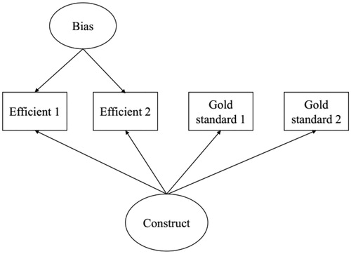
Data from the TMM design are analyzed using structural equation modeling, specifically a bias correction model (Graham et al., 2006; Graham & Shevock, 2012; Rhemtulla & Hancock, 2016). In the measurement model, observed variables from both the gold standard and the efficient measures all load onto a single latent factor. Additionally, a latent factor representing response bias is specified for the efficient measures only, which accounts for reporter-specific bias. Through use of Full Information Maximum Likelihood, measurement parameters are estimated, and a factor score for the primary construct of interest can be estimated for every participant, not just those who received the gold standard measures. To illustrate, an example of the bias correction model is presented in Figure 1. In the TMM, every participant would have observed data for the first two observed measures “Efficient 1” and “Efficient 2.” While a only a small subset of participants would have data for the other two measures “Gold Standard 1” and “Gold Standard 2.”

Figure 1. Example measurement model representation of the data collected in a planned missing data research design. The two observed gold standard measures are only collected on a randomly selected subset of the sample, while everyone in the sample receives the efficient measure.

To reiterate, one of the main benefits of the TMM design is the cost savings provided by only requiring a subset of participants to receive the most costly gold-standard assessments. Cost minimization is a feature of all planned missingness designs, of which the TMM is only one example (Graham et al., 2006). Readers may be familiar with the practice of using alternate forms of surveys with subsets of participants. Called the two-form or multi-form design, each form contains only a subset of the total items, reducing the participants’ total time investment. Another example of a planned missingness design is the wave missingness design, where a subset of participants are randomly assigned to not receive an assessment at a particular data collection point (see Rhemtulla & Hancock, 2016 for a review of planned missingness designs). With any planned missingness design, data are typically analyzed using maximum likelihood estimation or multiple imputation to fill in the missing data and obtain estimates with the total sample size, even those for whom data was not collected.

The TMM design has two distinct advantages over other types of planned missingness designs. First is the use of latent variables. Constructs are generally considered to be measured more accurately and with minimal error when they are measured in multiple ways, and preferably with multiple methods and/or by multiple reporters or raters (e.g., Bollen, 1989, 2002). The use of latent variables with multiple methods is inherent to the TMM design. Second, the TMM allows for a combination of the high-quality gold standard measures and the relatively lower-quality efficient measures in a way that capitalizes on the advantages of both types of measures. The increased sample size afforded from the use of the efficient measures improves the effective sample size, and therefore the statistical power of the study. The use of gold standard measures allows for the response bias associated with the efficient measures to be modeled, estimated, and accounted for using the described bias correction structural equation model. In sum, this results in better estimates of the overall construct, with improved statistical power compared to either standard data collection procedures.

Previous Applications of the TMM

The TMM design has been successfully demonstrated through both simulation studies (Graham et al., 2006) and applied studies (e.g., Drake et al., 2013; Zawadzki et al., 2012). For example, with simulated data on cigarette smoking, Graham et al. (2006) varied reliabilities of measures, cost differentials between gold standard and cheap measures, and effect sizes of major interest in a series of simulation studies. They found that compared to the complete-cases design, the TMM design produces higher efficiency and effective sample size (the sample size required to achieve the same statistical power as a complete-cases design). In other words, you can achieve the same effective sample size but at a lower cost because fewer participants have received the expensive gold standard measures. Drake et al. (2013) used empirical data of obesity based on both self-reported (an efficient measure) and objectively measured (the gold standard measure) height and weight. They reported that the TMM design yielded accurate and precise parameter estimation in this setting. Zawadzki et al. (2012) arrived at a similar conclusion when applying the TMM to an empirical example of blood pressure as predicting a health outcome. Together, these empirical examples demonstrate that the TMM methodology is excellent for simultaneously enhancing statistical power and reducing costs in a planned research.

Longitudinal Models

Longitudinal research designs add additional costs and efforts to the data collection process, and thus a data collection design that strikes a balance between statistical power and accuracy is in even greater need. Drawing from these concepts, Garnier-Villarreal, Rhemtulla, and Little developed a longitudinal extension of the TMM design (2014). Just as with the original TMM, the gold standard measure is only administered to a subset of participants at each timepoint (they also posit that it could potentially be administered at only a subset of occasions as well). To analyze the data, this method calls for fitting the bias-correction model separately at each measurement occasion, and then combining the two models into one simultaneously estimated model, with the latent variable representing the first timepoint directly predicting the second via a direct path.

However, the inclusion of additional time points of data collection poses several new conceptual challenges. Like all longitudinal models, constructs must be demonstrated to measure the same underlying construct at each measured time point (i.e., to be “invariant”). As an example, if observed variable A has a strong factor loading to the latent variable at the first time point, but a weak factor loading to the latent variable at the second time point, then we would conclude that the two latent factors do not represent the same thing (i.e., they are “non-invariant”); the latent variable would be more representative of observed variable A at the first measurement occasion than the second measurement occasion. Any attempt to examine how much change in the construct has occurred would be undermined, or biased, because the two latent variables represent something different.

This same idea can also extend to the bias factor, which may or may not be considered to be invariant across time. These ideas were explored by Garnier-Villarreal et al. (2014), who simulated data at four time points and varied the characteristics of response bias associated with the efficient measure, the factor structure of the response bias (unifactorial, multifactorial across time), constraints on model parameters, the number of occasions the gold standard measure was given, and the proportion of respondents administered the measure. They draw some conclusions related to the design of the study (e.g., if the bias factor is the same over time the gold standard measure only needs to be collected at one time point). However more relevant to the present study are the conclusions drawn around how the resulting data should be analyzed. Specifically, Garnier-Villarreal et al. (2014) conclude that a weakness of their study is that they did not have any applied data, and so it is unclear just how such biases would perform over time. Therefore, they conclude that questions about longitudinal equivalence and bias factor structure cannot be pre-determined, and rather should be tested when fitting a model to ensure that the most accurate representation of the data is identified. In the present study, we provide such an application, and demonstrate explicit steps including Mplus code, for those seeking to use this method in their own research.

Intervention Designs

Examining development is only one possible application of the TMM design. In addition, we assert that examining intervention effects is another natural extension of the model. In the longitudinal TMM, the core construct at the first measurement occasion is modeled with a predictive path to the core construct at the second measurement point (Garnier-Villarreal et al., 2014; Rhemtulla & Little, 2012). If a predictor variable representing participant assignment to treatment condition is added to that base model, it conceptually mirrors the regression-based ANCOVA framework commonly used for testing intervention response. In these models, performance at a second time point is predicted from performance on the same construct at the first time point, along with a variable representing the assigned treatment condition (Allison, 1990; Petscher & Schatschneider, 2011; Thomas & Zumbo, 2012; Zumbo, 1999). A scan of the recent issues of the Journal of Research of Educational Effectiveness demonstrates that such designs are commonly used to assess treatment effects in educational research, with regression (e.g., Murphy et al., 2020), hierarchical linear or mixed-effects models (e.g., Gandhi et al., 2020), and Structural Equation Models (e.g., Wanzek et al., 2020). Therefore in the present work, we provide an extension to the existing literature on planned missing designs to demonstrate how to measure intervention response within the longitudinal planned missing data framework.

Additional Assumptions for Causal Inference

Researchers are likely familiar with the practice of using a variable representing an assigned treatment condition as a predictor of a measured outcome as an estimate of the effect of that treatment. They may be less familiar with the assumptions and history that underlie this practice. Any time such an analysis is conducted, it is done based on the concept of the Neyman-Rubin potential outcomes model (e.g., Rubin, 1974). The term “potential” refers to the fact that an outcome cannot be observed for any one individual both when they were exposed to the treatment and when they were not exposed to the treatment. We can only observe one. Methodological researchers have developed several different designs to accommodate the need for this counter-factual comparison (see Shadish et al., 2002).

The most straightforward method of estimating the effect of treatment relies on the random assignment of participants to treatment conditions. Through random assignment, the groups of participants are equated on expectation; distributions of individual differences in traits or skills are assumed the same in each group. Using randomization ensures that the treatment assignment is independent of the potential outcomes; that the differences we observe between the two groups can only be attributable to the treatment. With two equal groups established through random assignment, comparing the mean of the group that did receive the treatment to the mean of the group that did not receive the treatment provides an estimate of the Average Treatment Effect (ATE), assumed to be the aggregate or average of each individual treatment effect. The control group serves as a stand-in for what would have happened to the treatment group if they had not received the treatment. For a causal inference to be valid, it must also meet the Stable Unit Treatment Values Assumption (SUTVA; Imbens & Rubin, 2015). This is the assumption that the intervention (treatment) is the same (stable) for all people who receive it (units). This means both that the people who are assigned to treatments do not interfere with one another, and that there is only a single version of each treatment. If this assumption is not met, then the potential outcomes are not uniquely identified, so the causal inference can be biased. Though several extensions to Rubin’s causal model exist to accommodate more complex quasi-experimental designs (Shadish et al., 2002), or individual treatment effects (Steyer, 2005), in the present study, we focus on this most simple methodology of estimating the average treatment effect. In this study, we use the TMM to estimate the difference in the means of a given outcome between a randomly assigned treatment group and a randomly assigned control group.

Just as with measuring latent constructs over time, it is important to determine whether measurement of the examined latent construct is invariant between treatment conditions. If treatment conditions have been assigned randomly, then any differences between groups should also be randomly distributed; the groups are equal on expectation at the pretest (Shadish et al., 2002). Through the process of growth and change, particularly the differential change that may occur between conditions, measurement non-invariance may be introduced. Making a valid inference regarding treatment effects depends on sufficient measurement equivalence between treatment arms because measurement nonequivalence may indicate that differences in means of the factors representing constructs are simply the result of difference in functioning on the indicators. Therefore, to fully extend the model to allow for causal interpretations, we must also test for the invariance of the differences between the treatment and control groups.

In summary, planned missingness designs provide researchers a method to measure a subset of people with expensive gold-standard assessments, while maximizing power and obtaining accurate estimation for a much larger total sample. Work by Garnier-Villarreal et al. (2014) proposed a longitudinal application of the TMM design, and demonstrate through simulation studies that it is an efficient and accurate tool for longitudinal research. However, to date, no empirical applications of the model have yet been published. The goal of the present study is to (a) inform the planned missingness design literature by providing an empirical application of the model, (b) to extend the model for use within intervention response research design framework, and (c) to provide researchers with step-by-step instructions for fitting longitudinal TMM models to their data, including how to estimate treatment effects from a longitudinal randomized control trial.

Method

Data

For the current investigation, we needed a data set that included both a gold-standard and an efficient measure of the same construct. We also needed a longitudinal sample that included at least two measurement points. Finally, we also wanted to investigate how to model treatment response within a longitudinal planned-missing data framework, therefore we needed a dataset that included random assignment to treatment. We searched through several databases at the Inter-University Consortium for Political and Social Research (ICPSR), and we selected to use the Sit Together and Read in Early Childhood Classrooms in Ohio (STAR2) study as the project provided a sampling frame that aligned with our research questions (Justice, 2017).

The STAR2 analytic sample consists of 693 preschool children from 83 early childhood special education (ECSE) classrooms with an average of 8.3 students per classroom. The STAR2 project was a randomized control trial (RCT) of the effectiveness of a 30-week book reading program implemented from 2008 to 2012. STAR2 was a cluster-randomized trial, with random assignment of participants to conditions conducted at the classroom-level. Teachers and caregivers were assigned to one of three conditions: (1) regular reading, in which teachers and caregivers were provided with storybooks and asked to read with their children on a given schedule, this served as the control group (2) print referencing, which included the same storybooks as the regular reading condition, but teachers were also asked to read the books while discussing print-related objectives and (3) print referencing and parental involvement group, which was the same as the print referencing group, but parents were also asked to read the storybooks following the same print-related objectives. More details of the study procedures can be found in Justice et al. (2015).

Specific to the present investigation, the STAR2 study measured all enrolled children in the classroom using efficient teacher-report measures of children’s language skills in both the fall and the spring of the academic year (approximately 7 months apart). Gold standard measures were administered to a purposefully selected sub-sample of children identified as having a language impairment (42% of the sample) on this same schedule. To distinguish those children with language impairments from their typically developing peers, (or peers with disabilities that did not affect language), teachers completed a brief screening questionnaire about each child. Though previous applications of the TMM have relied random assignment to missingness conditions, such that the participants who do not receive the gold standard are MCAR, the present study had purposefully selected missingness. The missing data in this study are therefore MAR, as the missingness is dependent on the results of the aforementioned screening questionnaire.

Sample Characteristics

The sample of children was primarily male (35% female). Just over half 56% had an individualized education plan (IEP), 77% were White, and had a mean age of 52 months (SD = 7.2). Just under half of the parents in the sample (44%) had a bachelor's degree or higher education. In terms of intervention group membership, 34% were from the regular reading group, 33% were from the print referencing group, and 33% from the print referencing and parental involvement group.

Measures

Language Skills

Children’s language skills were measured using the Comprehensive Evaluation of Language Fundamentals–Preschool (CELF: P-2; Wiig et al., 2004). Data from the fall and spring of the academic year were included in this study. The gold standard measures are comprised of expressive and receptive language skills from CELF: P-2. Expressive language (EL) is a composite score calculated from the subtests of expressive vocabulary, word structure, and recalling sentences. Receptive language (RL) is a composite score calculated from the subtests of basic concepts, concepts and following directions, and sentence structure. The efficient measures are comprised of nonverbal communication (NV), conversational routines and skills (CS), and asking for, giving, and responding to information (AG) using the Descriptive Pragmatics Profile (DPP) of CELF: P-2. The DPP is a teacher-report measure of children’s language ability rated on a 4-point scale (1 = never, 4 = always).

Intervention Variables

Intervention comprised two dummy coded variables, representing the two treatment arms. The first level of intensity was the print referencing group (Treatment A). The second level of intensity added print referencing with parent involvement (Treatment B). As previously stated, the regular reading group is the control group in this study. Estimates of intervention effects are made by including these two dummy variables in the model simultaneously. Coefficients for each represent the difference in the outcome between that intervention group and control.

Covariates

Child characteristics serving as covariates were whether the child had an individual education plan (IEP, 1 = yes, 0 = no), whether the child was White or not White (White, 1 = yes, 0 = no), and the mother’s level of education, coded as whether the parent had a Bachelor's degree (Education, 1 = yes, 0 = no).

Analysis

The primary aim of the present study is to illustrate the TMM with longitudinal data with a randomized treatment. We follow a four-step process based on recommendations by Garnier-Villarreal et al. (2014): In step 1, we fit the latent TMM model for each measurement occasion separately, pretest (fall) and posttest (spring). In step 2, we link the TMM models across time and determine the number of response bias factors needed. Step 3, we test longitudinal invariance of the substantive construct. Finally, in step 4 we demonstrate how to add predictors to assess intervention effects. All the steps were implemented using Mplus 7.3 (Muthen & Muthen, 1998–2012). Each step serves as the foundation for the subsequent steps. Details for each step are explained in the next section, and the corresponding annotated Mplus codes are provided in the appendix.

Step 1

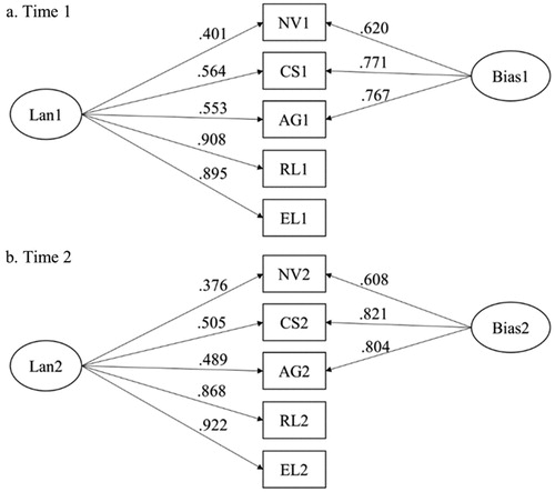
The first step investigates whether the two-method measurement (TMM) model provides reasonable fit to our data at each measurement occasion. Bias correction models, within the framework of SEM, were fit for the language variables at each time point separately. As illustrated in Figure 2, and taking Time 1 as an example, the model posits that both gold standard measures of receptive language and expressive language (RL1, EL1) and teacher-report measures of nonverbal communication, conversational routines and skills, and asking for, giving, and responding to information (NV1, CS1, and AG1) load on the core construct of language (Lan1). In addition, the three teacher-report measures load on the response bias factor (Bias1), which is independent from and not correlated with the construct factor. The models were evaluated by goodness of fit as detailed in the results section. If the bias correction model is supported for both time occasions, we can then proceeded to step 2. Because we seek to model a treatment effect, it is necessary to examine measurement invariance across treatment arms (for details, see Brown, 2015, pp. 259–265) to ensure that the latent mean differences across the group are interpretable.

Figure 2. Two-method measurement model for Time 1 and Time 2 with standardized estimates. Note. The two models (a and b) are fitted separately. Lan: language skill factor; Bias: response bias factor; NV: Nonverbal communication; CS: Conversational routines and skills; AG: Asking for, giving and responding to information; RL: receptive language standard score; EL: expressive language standard score. 1 or 2 indicates time points. All the loadings are significant at p < .001.

Step 2

In the second step, we fit the longitudinal TMM model was performed. Consistent with the method outlined in Garnier-Villarreal et al. (2014), competing longitudinal models were compared first to determine the nature of the response bias factor. Generally, researchers have two options when considering the bias correction model in a longitudinal framework. First, separate bias estimates could be fit, one for each time point. A second option is to treat bias as un-changing over time and fit a model constrained to have one bias factor for all efficient measures across the observed time points (Garnier-Villarreal et al., 2014).

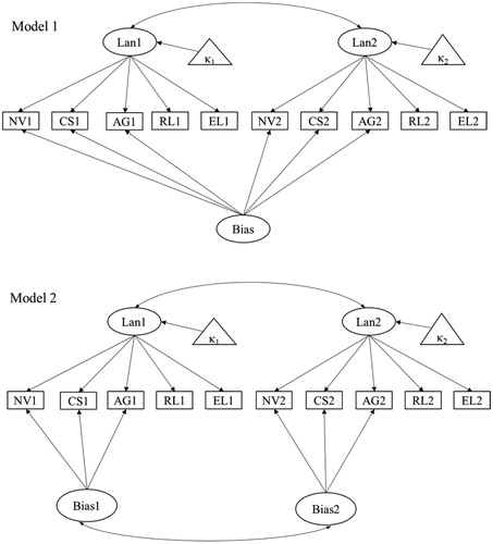
As depicted in Figure 3, Model 1 posits one bias factor underlying the efficient measures across time, whereas Model 2 posits a separate response bias factor for each time point. In both models, latent factors and item residuals are allowed to covary with their counterparts across time to account for the correlation between constructs. Since Model 1 and Model 2 are nested (fix the bias factor correlation across time in Model 2 to be 1 yields Model 1), model comparison can be conducted based on chi-square difference (Δχ²) test, along with other fit indices detailed in the next text. After the model with better fit was identified and hence the number of bias factors was determined, we can proceed to step 3.

Figure 3. Competing two-method measurement models for longitudinal data. Error covariances for corresponding indicators across time are added but not shown. Lan: language skill factor; Bias: response bias factor. NV: Nonverbal communication; CS: Conversational routines and skills; AG: Asking for, giving and responding to information; RL: receptive language standard score; EL: expressive language standard score. 1 or 2 indicates time points. κ₁, κ₂ refer to the mean structure at Time 1 and Time 2.

Step 3

The third step examines whether the meanings of the latent core constructs are comparable across time. Longitudinal invariance was assessed through a series of nested models with increasing degree of constraints, Model 3_a and Model 3_b. In Model 3_a (metric invariance), factor loadings of the core construct are constrained to be equal across time. In Model 3_b (scalar invariance), indicator intercepts are constrained to be equal across time. Models are evaluated in the same manner as that of step 2. Supportive evidence of longitudinal invariance would indicate that it is meaningful to compare latent language skills before and after the intervention.

Step 4

The next step builds from the final bias corrective longitudinal model to examine the effects of an intervention on children’s language skills at Time 2 controlling for the baseline language skill, and children’s background information. All the measurement models and SEM models were estimated using the full information maximum likelihood estimation method to accommodate the planned missingness. Moreover, since students are nested within classrooms, the Mplus command of type = complex, which calculates robust variance and test statistics through a sandwich estimator (see Muthen & Satorra, 1995 for technical details), was adopted for all the models to account for the dependence shared by students within each cluster.

Evaluation Criteria

Model performance was evaluated by χ² test, comparative fit index (CFI), Tucker–Lewis index (TLI), root mean square error of approximation (RMSEA), and root mean square residual (SRMR). Values of greater than .95 for CFI and TLI, lower than .06 for RMSEA, and close to .08 for SRMR are considered satisfactory model fit (Hu & Bentler, 1999). In addition, model comparisons for the nested longitudinal TMM models were assessed by Δχ² test, combined with ΔCFI and ΔRMSEA given the sensitivity of Δχ² test toward sample size. A significant difference in nested models is indicated by a p value of < .001 for the Δχ² test, a ΔCFI of < .01, and a ΔRMSEA of > .015 (Chen, 2007).

Results

Descriptive Statistics

The descriptive statistics and Pearson correlations of the main variables are displayed in Table 1. The three teacher-reported measures, NV, CS, and AG were positively and highly correlated with each other at both time points, indicating high internal consistency. Similarly, the two gold standard measures, RL and EL, were highly related. Additionally, the teacher-reported measures were positively and moderately associated with the gold standard measures. All the correlations were significant at p <.001. Moreover, the means of all the language measures were higher at Time 2 compared to Time 1, indicating growth in learning.

Table 1. Pearson correlations, means, and standard deviations of the language measures across time (N = 693).

	Efficient (Pre)			Gold standard (Pre)		Efficient (Post)			Gold standard (Post)
	NV1	CS1	AG1	RL1	EL1	NV2	CS2	AG2	RL2	EL2
NV1	—
CS1	0.704	—
AG1	0.697	0.904	—
RL1	0.365	0.473	0.466	—
EL1	0.279	0.468	0.455	0.801	—
NV2	0.594	0.499	0.506	0.374	0.288	—
CS2	0.554	0.765	0.740	0.457	0.422	0.689	—
AG2	0.553	0.721	0.755	0.455	0.421	0.673	0.907	—
RL2	0.303	0.390	0.373	0.772	0.742	0.347	0.420	0.419	—
EL2	0.283	0.486	0.450	0.744	0.856	0.308	0.456	0.435	0.798	—
M	23.537	33.667	18.683	78.018	75.128	24.961	37.579	21.317	79.799	80.343
SD	4.844	8.589	5.543	17.010	16.909	4.204	8.297	5.404	17.921	17.826

Note. All the correlations are significant at p < .001. NV: Nonverbal communication (1 or 2 indicates time points); CS: Conversational routines and skills (1 or 2 indicates time points); AG: Asking for, giving and responding to information (1 or 2 indicates time points); RL: receptive language standard score (1 or 2 indicates time points); EL: expressive language standard score (1 or 2 indicates time points).

Step 1: TMM Model Fitting at Each Time Point

The construct validity of the TMM model was tested separately at both measurement occasions (see Mplus code for this step in the appendix). Results showed that both models displayed satisfactory fit to the data, χ² (2) = 7.226, p = .027, CFI = .996, TLI = 0.979, RMSEA = .062, SRMR = .010 for Time 1, and χ² (2) = 6.328, p = .042, CFI = .997, TLI = 0.983, RMSEA = .056, SRMR = .008 for Time 2. The TMM models with standardized coefficients are exhibited in Figure 2, and more detailed information of parameter estimates are displayed in Table 2. At Time 1, all the language measures positively and significantly (p < .001) loaded on the core construct Lan1 with moderate to high magnitude of loadings. Furthermore, all the three efficient measures positively loaded on the response bias factor Bias1.

Table 2. Factor loading estimates for the TMM models across time.

	Time 1						Time 2
	Lan1			Bias1			Lan2			Bias2
Item	λ_std	λ	SE	λ_std	λ	SE	λ_std	λ	SE	λ_std	λ	SE
NV	0.401	1.000	0.000	0.620	1.000	0.000	0.376	1.000	0.000	0.608	1.000	0.000
CS	0.564	2.498	0.330	0.771	2.207	0.154	0.505	2.648	0.360	0.821	2.666	0.230
AG	0.553	1.580	0.212	0.767	1.417	0.103	0.489	1.673	0.235	0.804	1.701	0.140
RL	0.908	8.183	1.244				0.868	9.886	1.760
EL	0.895	7.979	1.427				0.922	10.460	2.240

Note. λ_std: standardized factor loadings; λ: unstandardized factor loadings; SE: standard error. The p values for all the loadings are <.001.

The results revealed that Lan1 well captured the trait variance underlying the language measures, and Bias1 well explained the variance uniquely associated with the efficient measures. Importantly, the loadings of the two gold standard measures on the core construct were saliently higher than those of the efficient measures. For example, in the Time 1 model, the gold standard loadings were .908 and .895, while the efficient measures ranged from .401 to .564 (Figure 2). This finding is consistent with the expectation that the gold standard measures provide a more valid assessment of the core construct. The TMM model at Time 2 exhibited similar performance as Time 1, with the standardized loadings comparable across time, suggesting the final models for stage 1 were identified, and we could move to step 2: determining the nature of the bias factor. It is worth mentioning that because our study involves testing a treatment effect, measurement invariance across the three treatment arms was also examined. The results showed that scalar invariance across group was satisfied for both measurement occasions, CFI = .997, TLI = 0.985, RMSEA =.054, SRMR = .013 for Time 1, and CFI = 1.000, TLI = 1.009, RMSEA = 0, SRMR = .009 for Time 2 (not presented), suggesting that it is meaningful to compare latent means across group.

Step 2: Determine the Number of Response Bias Factors

In order to determine the optimal longitudinal TMM model, two competing models were examined. As shown in Figure 3, Models 1 and 2 share the same model specification except for the response bias factors: Model 1 posits that the teacher-reported measures share the same bias factor across time, while Model 2 frees this assumption and estimates separate bias factors on each measurement occasion. In both models, paired item residuals are allowed to covary across time, which is not shown in the figure (for a detailed illustration of longitudinal invariance modeling, see Brown, 2015, pp. 221–234). In addition, the variance of Lan1 is constrained to 1 for both models to facilitate comparison of the variance of the language construct across time. As reported in Table 3, the model fit indices for Model 1 were CFI = .914, TLI = 0.839, RMSEA =.136, SRMR = .191. The RMSEA and SRMR indices suggest that Model 1 does not provide a good fit to the data. The goodness of fit for Model 2 were CFI = .993, TLI = 0.987, RMSEA =.039, SRMR = .071, indicating a satisfactory model fit. Moreover, the χ² difference test for Model 2 vs Model 1 was significant (p < .001), and differences in CFI (ΔCFI = 0.079) and RMSEA (ΔRMSEA = −0.097) were greater than .01, indicating that Model 2 fitted significantly better than Model 1. Therefore, the optimal longitudinal TMM model was determined to have a separate response bias factor at each measurement occasion.

Table 3. Model comparisons for the longitudinal TMM models.

Model	χ^2	df	CFI	TLI	RMSEA	SRMR	p of Δχ^2	ΔCFI	ΔRMSEA
Model 1	331.391	24	0.914	0.839	0.136	0.191	—	—	—
Model 2	47.115	23	0.993	0.987	0.039	0.071	<.001	0.079	−0.097
Model 3_a	47.254	27	0.994	0.991	0.033	0.082	0.766	0.001	−0.006
Model 3_b	141.485	31	0.969	0.955	0.072	0.106	<.001	−0.025	0.039
Model 3_c	48.880	29	0.994	0.991	0.031	0.094	0.364	0.000	−0.002

Note. p of Δχ²: p value of χ² difference test. ΔCFI: difference in CFI; ΔRMSEA: difference in RMSEA. Model 1 = longitudinal model with single bias factor; Model 2: longitudinal model with separate bias factors; Model 3_a = metric invariance across time; Model 3_b = scalar invariance model; Model 3_c = partial scalar invariance model.

Step 3: Longitudinal Invariance of Language Skills

Subsequently, based on Model 2, longitudinal invariance was tested by imposing equality constraints on the factor loadings on the core construct across time (referred to as Model 3). This step constitutes the prerequisite for a meaningful comparison of latent language skills across time. As shown in Table 3, Model 3_a indicated an acceptable model performance. Moreover, the χ² difference test for Model 3_a vs Model 2 was not significant, and differences in CFI and RMSEA were less than .01, indicating that Model 3_a does not fit significantly worse than Model 2. Therefore, metric invariance for the longitudinal TMM model was supported.

Comparing Model 3_b versus Model 3_a, the χ² difference test was significant, and the differences in CFI and RMSEA were greater than the suggested cutoffs, suggesting that scalar invariance is not fully satisfied. Based on the information from modification indices, a partial scalar invariance model was further examined (denoted as Model 3_c) which set free the intercept constraints across time for two indicators. As shown in Table 3, Model 3_c has acceptable model performance, and compared to Model 3_a, the χ² difference test was, and the differences in CFI and RMSEA are less than .01, suggesting that the partial scalar invariance model is acceptable. The corresponding estimates are shown in Table 4.

Table 4. Parameter estimates for longitudinal invariance model.

	Lan1			Bias1			Lan2			Bias2
Item	λ_std	λ	SE	λ_std	λ	SE	λ_std	λ	SE	λ_std	λ	SE
NV1	0.208	1.000	0.000	0.709	1.000	0.000
CS1	0.380	3.150	0.415	0.870	2.110	0.116
AG1	0.388	2.077	0.263	0.862	1.351	0.077
RL1	0.860	14.654	0.974
EL1	0.933	15.687	1.182
NV2							0.251	1.000	0.000	0.661	1.000	0.000
CS2							0.406	3.150	0.415	0.875	2.576	0.193
AG2							0.411	2.077	0.263	0.841	1.613	0.126
RL2							0.856	14.654	0.974
EL2							0.928	15.687	1.182
Means	23.675	23.675	0.310				23.828	24.896	0.291

Note. λ_std: standardized factor loadings; λ: unstandardized factor loadings; SE: standard error. The p values for all the loadings are <.001. Means refer to the latent language skill mean estimates. Lan1 and Lan2 are correlated at .938, p < .001; Bias1 and Bias2 are correlated at .754, p < .001. The variance for lan1 was fixed to 1 to facilitate interpretation, and the variance for lan2 is 1.092 (SE = 0.085, p < .001).

Step 4: Add Predictors to Estimate Intervention Effectiveness

To further investigate the utility of the TMM model in longitudinal research, we next sought to demonstrate how to test for the effects of an intervention on Time 2 language skills after controlling for Time 1 language skills and background information. The model was identical to Model 2 (from Figure 3), except that additional observed variables were added: one for each covariate (IEP status, White, and Education), and one representing membership in each of two different conditions (Treatment A: print referencing or Treatment B: print referencing with parent involvement). Those observed variables all loaded on the Language variables, both at Time 1 and Time 2. Paths from the treatment variables to language at the first time point serve to establish baseline equivalence, while those to the Time 2 language construct estimate the treatment effect: The predicted difference between that condition and the control group on the post-test, after controlling for the pretest and covariates.

The SEM showed satisfactory fit to the data, χ² (63) = 83.187, p = .045, CFI = .994, TLI = 0.991, RMSEA = .023, and SRMR = .037. The factor loadings for the measurement model were consistent with those in the previous steps (Table 4), and Bias1 and Bias2 were correlated at .680 (p < .001). The parameter estimates for the structural part of the model are presented in Table 5. In Table 5, the rows represent the predictors, and the columns represent the endogenous variables in the SEM model (Language at Time 1, Language at Time 2, Bias at Time 1 and Bias at Time 2).

Table 5. Parameter estimates of the final SEM with assigned treatment group predicting Language at time two.

	Lan1				Lan2				Bias1				Bias2
Predictor	β	B	SE	p	β	B	SE	p	β	B	SE	p	β	B	SE	p
Lan1	—	—	—	—	0.998	0.967	0.043	<.001	—	—	—	—	—	—	—	—
Group A vs. Control	0.042	0.114	0.188	.547	0.020	0.052	0.093	.576	—	—	—	—	—	—	—	—
Group B vs. Control	−0.079	−0.216	0.153	.155	0.084	0.224	0.109	.043	—	—	—	—	—	—	—	—
IEP	−0.520	−1.346	0.342	<.001	0.116	0.291	0.226	.219	−0.369	−2.280	0.482	<.001	−0.405	−2.047	0.482	<.001
White	0.231	0.701	0.148	<.001	0.038	0.113	0.087	.204	0.032	0.230	0.401	.563	−0.025	−0.145	0.281	.605
Education	0.198	0.511	0.147	<.001	−0.009	−0.022	0.064	.733	−0.082	−0.507	0.286	.073	−0.058	−0.293	0.241	.213

Notes. β: Standardized estimates; B: Unstandardized estimates; SE: Standard error.

For Language at Time 1, no significant intervention group differences were found, indicating that the study demonstrates baseline equivalence. All three background variables were significantly related to Lan1, indicating that the students who were White, with higher parental education level, and who did not have an IEP had higher language performance at Time 1.

We next examined whether the bias factors were related to background characteristics. In terms of the effects on the response bias factors, IEP was significantly and negatively related to both Bias1 (β = −0.369, B = 2.280, SE = 0.482, p < .001) and Bias 2 (β = −0.405, B = 2.047, SE = 0.482, p < .001), while the other background variables did not significantly relate to response bias. This indicates that teachers showed significantly less response bias, and were more accurate at rating the language skills of those children with an IEP.

The primary results of interest with this model are predictions relevant to the second time point. First, the autoregressor (Lan1) significantly and positively predicted Lan2 (β = .998, B = .967, SE = .043, p < .001), indicating a high stability over time. In terms of intervention effects, Treatment B significantly predicted Lan2 (β = .084, B = .224, SE = .109, p = .043) while Treatment A did not. This suggests that students who participated in the print referencing and parental involvement intervention group showed significantly more growth in language compared to students in the regular reading condition, after controlling for the effects of baseline performance and background information. Moreover, none of the background variables had significant effects on Lan2, suggesting that the growth in language skills was not due to students’ demographic background.

Comparison to Gold Standard Only Model

At the suggestion of anonymous reviewers, we next compared the results of the longitudinal TMM treatment effects model to a model where the gold standard measures were included as the only indicators of the latent variables at each language time point. This contrast serves to demonstrate the gains in specificity afforded by the inclusion of the larger sample size of efficient measures. The gold standard only model was similar to the final SEM model in step 4 except that the latent construct of language skill was only represented by the gold standard measures of RL and EL, and we did not include a response bias factor. This model was the same for both time points. The latent variable at Time 1 was specified to predict the latent variable at Time 2. The variables representing the intervention group, as well as the covariates of IEP, White, and Education were specified to predict the latent variables at both time points, as was the case with the longitudinal TMM treatment effects model. The model provided satisfactory fit to the data, as shown in the footnote of Table 6. Contrasting the intervention effect results in Tables 5 and 6, particularly for the effect of Group B vs Control on lan2, the SE from the gold standard only model was noticeably larger than that of the TMM model (SE of 1.259 vs 0.109). The results demonstrate that there is less estimation precision with the gold standard only model compared to the longitudinal TMM.

Table 6. Comparison for gold standard only SEM with assigned treatment group predicting language at Time 2.

	Lan1				Lan2
Predictor	β	B	SE	p	β	B	SE	p
Lan1	—	—	—	—	0.934	0.978	0.046	<.001
Group A vs. Control	0.119	3.650	2.565	.155	0.002	0.076	1.218	.950
Group B vs. Control	−0.031	−0.915	2.173	.674	0.070	2.169	1.259	.085
IEP	−0.118	−11.093	3.257	.001	0.036	3.560	2.568	.166
White	0.288	9.831	1.867	<.001	0.038	1.373	1.149	.232
Education	0.204	5.846	1.796	.001	−0.015	−0.441	0.801	.582

Note. The model fits well, χ² (11) = 9.201, p = .603, CFI = 1.000, TLI = 1.005, RMSEA = .000, SRMR = .016.

Discussion

The present study had three overarching aims. First, to inform the literature of planned missingness designs by examining how such models perform in empirical data. This study has demonstrated that the efficient and gold-standard measures selected here provided an excellent fit to the data, and provides good evidence that such models are viable for use in developmental contexts. However, the final model we demonstrate here was not the first one that we estimated. The foundational work by Garnier-Villerreal et al. (2014), left open the question of the necessary number of gold standard indicators, and explicitly suggested that a single gold standard measure may be sufficient (p. 421). Based on this guidance, we first attempted to include a single gold standard measure at each time point. However, this model had considerable estimation problems (e.g., negative residual variance). When we added a second observed gold-standard measure, we encountered no estimation issues. Presumably, this is due to increased model stability associated with additional manifest variable indicators on the two latent language factors. Therefore, our first conclusion of the present study is that a minimum of two gold standard measures is necessary for the successful estimation of the TMM model.

An additional question that remained from Garnier-Villerreal et al.’s (2014) work was how bias would function over time. Though the teacher-rating scale used in the present study was administered by the same teachers at both time points, the bias was still best captured by estimating separate factors at each time point. We recommend that future researchers who seek to use the longitudinal TMM design err on the conservative side when planning data collection; plan the study as if two bias factors will be required. Operationally, this means that the gold-standard measure should be included at both time points rather than just one.

One additional point to consider is that the present study used a well-established and well-validated teacher-report measure. This has implications for generalization to other studies in two ways. First, teachers are professionals who are used to thinking about questions related to children’s development. Professionals are more likely to provide valid responses to any given scale, provided it is within their area of expertise (e.g., nurses rating patient symptomology). This is less likely to be the case when the rater is not a professional within the area that they are rating. For example, teachers spend relatively less time thinking about children’s friendships, therefore we might expect that teacher ratings of children’s friendships may be less accurate (show poorer factor loadings and higher bias) than the constructs we examined in the present study. Second, many efficient rating scales do not share the strong psychometric properties of the scale used in the present study. It is well established that scales with better internal consistency and reliability provide a better estimation of the true overall latent construct, as evidenced through stronger factor loadings (Bollen, 1989, p. 221). Therefore the model may not fit as well if the measures used to assess the efficient or gold-standard measure are not as psychometrically sound as those included here.

To illustrate the TMM, the present study used a cluster robust standard error estimator to address the nested nature of the data. However, we also relied on a teacher-report assessment as our efficient measure, and as such these ratings may have affected children’s outcomes in other ways. With one teacher rating several students, it is possible that the measurement structure may have differed between raters, or that responses may have been dependent on children’s classroom performance in other ways. Though our bias factor is designed to capture some of these possibilities, it is unable to account for others. Future studies should investigate whether a multilevel or mixed model extension of the TMM design can be developed that would better account for this shared variance. Until that time, researchers who are in the planning stages of their research projects should consider relying on assessments that do not have issues with nesting. Measures that rely on self-report or parent-report for example, afford researchers the advantages of an additional rater as part of their efficient measure, but do not have the issues of the same person providing ratings for multiple participants.

A potential weakness of the present study is that the demonstration dataset did not use random assignment to select who would receive the gold standard assessments. Instead, this project relied on a purposefully selected sample; the children who were selected for these assessments differed systematically from those children who were not selected. Thus, data for the unselected students are considered to be Missing At Random (MAR), these data are missing but for a reason we know and can predict or explain. In the handling of missing data for any standard analysis, data that are MAR can be analyzed or imputed without introducing bias, provided that the variables used to select or predict the missingness are included as auxiliary variables during analysis or data generation (Puma et al., 2009). The theoretical work behind the TMM explicitly relies on an assumption of random assignment to missingness conditions, such that the data for the unselected sample (the participants who do not receive the gold standard assessments) are Missing Completely At Random (MCAR). An important direction for future work would be to investigate the extent to which the MCAR assumption can be relaxed in the TMM design and still allow for unbiased estimates. The ability to use a set of gold standard assessments with a purposefully selected sample (as was used in this illustration) would be extremely beneficial with the needs of researchers focused on either gifted students or students with disabilities, and with school buildings and school districts who want to better understand their poorest performers.

An additional consideration is the method we used to assess growth in the present study. Though two-timepoint designs are common, they are often thought of as inferior to multiple-time-point growth models; models that explicitly estimate each person’s growth on the construct of interest (Cronbach & Furby, 1970; Curran et al., 2010). Another method of examining change between two or more timepoints is the latent change model (McArdle, 2001; Steyer et al., 1997). These models also explicitly estimate change via a latent variable that provides an estimate of growth for each individual person. However they are more flexible as they only require two measurement occasions to estimate change, while the growth model requires three or more. As of yet, the longitudinal TMM design has not been extended to fit within a growth modeling framework nor a latent change framework. This is a potentially important area of future research.

The second aim of this study was to provide an empirical example of whether the TMM design could be used to measure the average treatment effect in a residualized change format. Crucially, the TMM identified a significant effect of Treatment B compared to the Control condition, which was not observed when the gold standard measures were the only outcome measures included. Moreover, the present study empirically contrasted the standard errors (SEs) of parameter estimates yielded from the longitudinal TMM treatment effect model and its gold standard only counterpart. The results revealed that SEs yielded from the gold standard only model were generally larger than those from the TMM design, suggesting lower estimation precision and lower statistical power with the former model. This confirms previous similar findings on the size of standard errors in planned missing data designs as discussed in Graham et al. (2006). This finding demonstrates the potential of the longitudinal TMM design in retaining statistical power and estimation accuracy.

In addition, the present study only just began to explore the potential for causal modeling within the TMM framework. We provided an example of a randomized control trial, but there are several other kinds of quasi-experimental designs that could also be potentially fit into this framework. In addition, this model also has the potential to generalize to the work of Steyer (2005), and his adaptation of Rubin’s causal model from average treatment effects to individual treatment effects. This work relies on a similar structural equation model to the one presented in this study, including primary constructs and the estimation of a bias factor. Though this work has thus far has relied on complete data for all participants, it also has the possibility to be extended into a planned missing data framework.

The final aim of this work was to establish for applied researchers that the longitudinal TMM model is applicable for questions in developmental research and to demonstrate how the model can be fit to their data. Through providing example code and step-by-step instructions, we believe other researchers will be able to work through the model fitting process with relative ease. As with any empirical study, our results are limited in their generalizability. Specifically, other researchers who seek to fit these models may them more difficult to fit than what we describe here. Considering the reliability, consistency, raters, and measures selected, any of these may deleteriously influence the fit, and the chance of seeing errors of estimation, during the model fitting process. However, with this guide along with the foundational work in this area (e.g., Garnier-Villarreal et al., 2014), we believe that researchers will find these models more accessible than they have in the past.