Distribution free approach on electrical energy supply chain using geometric shipment policy

ABSTRACT

We propose an inventory based optimisation model for a system of electricity supply chain. This distribution system consists of power plant, transmission substation and distribution substations and customers. The electricity generated by the power plant is transmitted to the submission and distribution substations and finally consumed by the customers. We apply the ^inventory theory to the distribution system and assume the electricity demand follows a distribution-free approach. This distribution system concerns the geometric shipment policy that is the size of each shipment is a multiple of the first shipment size. In particularly, two types of lead time crashed concepts are considered in this model. The main objective of this model is to find an optimal solution of first shipment lot size, blackout cost and simultaneously minimising the joint expected total cost. An iterative technique is used to find an optimal solution numerically and a sensitivity analysis table is presented to show the impact of different parameters

KEYWORDS:

• Electrical energy supply chain
• distribution-free approach
• lead time reduction
• optimisation
• inventory control

1 Introduction

Generally, a supply chain inventory model defines the vendor–buyer relationship. Energy as a catalyst of development is an essential indicator in the development of manufacturing industry and society. Energy demand is rising day by day due to an increasing population and technological advancement in the industry. Globally a large share of energy demand is originating from the industrial sector and consuming a significant amount of energy. The total electricity consumption in worldwide is gradually increasing every year. Electricity consumption for industrial, commercial, residential and transportation sectors has been enhanced in recent decades. The world

energy consumption is gradually increasing due to several reasons such as air-conditioners at every home because of increasing climate changes, increasing technological equipments, battery-based cars, etc. The electricity price is being influenced by the demand for electricity already and unmanaged demand-supply can influence the price to go even high. In an electrical supply chain inventory system, following all activities are managed, electricity generated in a power plant will be transmitted through a transmission line and distribution substation to the customers. In a supply chain inventory system, the capacity of electrical energy has the same process for determining the order quantity and total cost.

2 Literature review

Worldwide consumption is expected to increase by 56$\mathrm{\%}$ between 2010 and 2040. The consumption of electricity will rise by 69$\mathrm{\%}$ from 21.6 trillion kilowatt-hours in 2012 to 36.5 trillion kWh in 2040 (Wangsa and Wee 2018). The industrial sector is the largest share of energy consumption. In the face of this projected growth, it is important to understand and manage the electricity supply chain system. (Fossati et al. 2015) proposed a genetic algorithm to minimise cost and optimise energy in micro-grid systems. (Luo et al. 2015) classified the electrical energy storage technologies into six forms of stored energy. The first study using a simple inventory model to analyse the electrical supply chain was conducted by (Schneidera et al. 2015), (Schneider et al. 2016). (Taylor et al. 2017) used a two-stage game theory model to study price and capacity competition in electricity market. (Wu, Philpott, and Zakeri 2017) derived a model to study the conventional generation with intermittent supply. (Ouedraogo 2017) developed an electricity supply-demand model for the African power systems. (Wangsa, Yang, and Wee 2018) proposed the effect of price-dependent demand on the sustainable electrical energy supply chain.

To improve customer service and to reduce stock out loss, it is important to reduce lead time. (Liao and Shyu 1991) first incorporated a probabilistic inventory model assuming lead time as a unique decision variable. (Ben-Daya and Raouf 1994) considered an inventory model as an extension of (Liao and Shyu 1991) model where lead time is one of the decision variables. (Ben-Daya and Raouf 1994), model dealt with no shortage and continuous lead time. (Ouyang, Yeh, and Wu 1996) extended (Ben-Daya and Raouf 1994) model by assuming discrete lead time and shortages. (Pan and Yang 2002) analysed an integrated inventory model with lead time in a controllable manner. (Annadurai and Uthayakumar 2010) developed a periodic review inventory model under controllable lead time and lost sales reduction.

(Goyal 1995) studied a model in which the shipment size increases geometrically. (Hill 1997) developed the (Goyal 1995) model where the geometric growth rate in shipments size is a decision variable. (Goyal and Nebebe 2000) presented geometric-then-equal-shipments policy for the first time. In this policy, the size of shipments is small at first and then its size growths by multiplying a factor and finally the shipment size will be constant for some shipments. (Hill 1997) studied a problem where there is no pre-defined assumption on the shipment delivery policy. He showed that the optimal shipment delivery policy is geometric-then-equal-shipments policy. (Goyal 1988) presented a generalised model in which the lot-for-lot policy is relaxed and insisted that vendor’s economic production quantity must be an integral multiple of buyer’s order quantity. Later, several researchers (Hoque and Goyal 2006), (Goyal and Nebebe 2000),(Pandey, Masin, and Prabhu 2007),(Teng, Cárdenas-Barrón, and Lou 2011),(Tsou et al. 2009) (Chen, Chang, and Ouyang 2001) have developed integrated production-distribution inventory models by extending the idea of (Goyal 1988) and incorporating various realistic assumptions. But it is not always suitable in a realistic environment.

Different researchers developed different types of model under the consideration of production systems with safety stocks and equal sized shipments but no one developed an integrated distribution system with unequal sized shipments for an electricity power system with stochastic electricity demand, transmission cost and distribution cost. In particular two types of lead time concept are considered which are lead time depends on the setup and transportation time and other is the lead time depends on transportation time only. Using the two types of lead time, most of the researchers considered a backorder quantity follows a normal distribution, uniform distribution, etc. But in this paper, we have considered a shortage cost follows a free distribution concept. An iterative solution technique is used to find an optimal solution numerically. An iterative method is a mathematical procedure that uses an initial guess to generate a sequence of improving approximate solutions for a class of problems, in which the $n-th$ approximation is derived from the previous ones. There is a big research gap in this direction, which is fulfilled by this research. In this paper, section 2 represents a problem definition, notations and assumptions, section 3 describes a mathematical model, section 4 describes the solution methodology of the model, section 5 represents the numerical example of the model and section 6 explains the sensitivity analysis and conclusion of the model.

2.1 Problem description, notations and assumptions

In this supply chain system, we consider an electricity power system with stochastic electricity demand, transmission cost and distribution cost. The power plant produces electricity to the customers and the power plant electricity production batch of size $Q$ which is made up of $n$ unequal-sized shipments which are transmitted to the customers. The customer has a stochastic lead time $L(P,Q)$ depends upon lot size and production of electricity. $L(P,Q)$ does not follow any particular distribution. $DL(P,Q)$ and $\sigma \sqrt{L(P,Q)}$ are known. $L(P,Q)$ depends upon transportation time and setup cost. In order to supply the electricity from the power plant to the customers, the transmission and distribution costs will be charged. The transmission and distribution costs are function of the maximum capacities of power plant, the transmission substation and the distribution substation, $(W_p^x,W_t^x,W_d^x)$. Finally, the expected total cost for the integrated model is calculated and some conclusions are drawn from numerical example.

2.1.1 Notations

We need the following notations and assumptions, to develop the mathematical model of this model. The following terminology is used:

Table

$Q$ Power consumption of the customers

$q_1$ Size of the first shipment from the power plant to the customer

$D$ Average of electricity demand rate of the customers

$P$ Power supply rate of the power plant $P>D$

$S$ Power plant’s setup cost per setup

$\lambda$ Geometric growth factor

$k_1$ Backup factor of batch 1

$k_2$ Backup factor of batch 2,3,,,m

$T_s$ Setup and transportation time

$T_t$ Transportation time

$g$ Electricity power distribution factor from the distribution substation to the customers

in one production cycle

$p$ Electricity power distribution factor from the transmission substation to the

distribution substation in one production cycle

$m$ Electricity power distribution factor from the power plant to the transmission

substation in one production cycle

$\sigma$ Standard deviation of electricity demand of the customers

$t$ Average of time consumption of the customers

$E$ Customers energy consumption, $(E=Q.t)$

$A$ Ordering cost of the customers

$E_c$ Electricity price of the customers

$C_p$ Production cost incurred by the power plant

$C_t$ Transmission and distribution rates paid by the power plant

$h_t$ Holding cost of the transmission substation

$h_p$ Holding cost of the power plant

$\pi$ Backorder cost per electricity consumption of the customers

$\delta$ power factor correction

$P_{dt}$ Transmission and distribution rates paid by the power plant

$D_d$ Distribution network from the distribution substation to the customers

$D_t$ Transmission network from the transmission substation to the distribution substation

$D_p$ Transmission network from the power plant to the transmission substation

$W_d^x$ Maximum capacity of distribution substation

$W_t^x$ Maximum capacity of transmission substation

$W_p^x$ Maximum capacity of power plant

$W_d^y$ Actual capacity of distribution substation

$W_t^y$ Actual capacity of transmission substation

$W_p^y$ Actual capacity of power plant

$\alpha$ Power supply loss factor

2.2 Assumptions

The fundamental assumptions used in developing the model are as follows:

1. This is a single-power plant, a single-transmission substation, a single-distribution substation and single-customer model.

2. The power plant produced the energy with a finite power supply rate $P$ ($P>D$) in units per unit time in one setup. Electrical energy are supplied to the customer in $n$ unequal sized shipments.

3. $Qt$ energy will be consumed by the customers (in kWh).

4. The power plant produces the electricity energy to the transmission substation of $Qtgpm$ (kWh) and supplies to the transmission substation of $Qtgn$ (KWh), supplies to the distribution substation of $Qtg$ (kWh), and supplies to the customer of $Qt$. (Wangsa and Wee 2018)

5. The maximum capacity of power generation must be greater than at the transmission and distribution substations $(W_p^x,W_t^x,W_d^x)$ in kVA.

6. In reality, it is not possible for an industry manager to find out the exact distribution function of lead time demand and after that solve the lead time problem. Whenever previous data is in stock, mean, i.e., average and standard deviation can be calculated. The buyers model considers a $(Q,S)$ continuous review inventory model with demand $D$. The demand $X$ during lead time $L(P,Q)$ follows a unknown distribution having known mean $DL(P,Q)$ and standard deviation $\sigma$ where $L(P,Q)$ is the lead time and depends upon setup and transportation time $(T_s)$ as well as and processing time $\frac{Q}{P}$. (i.e.,)$L(P,Q)=T_s+\frac{Q}{P}$.

7. If lead time is high, then lost sale increases which cause a huge loss to the industry. The known mean and standard deviation of lead time demand are $DL(P,Q)$ and $DL(T_t)$ and the corresponding standard deviation as $\sigma \sqrt{L(P,Q)}$ and $\sigma \sqrt{L(T_t)}$ respectively. Thus the safety backup supply for the first batch is,

$s_1=k_1\sigma \sqrt{L(P,Q)}=k_1\sqrt{T_s+\frac{Q}{P}}$

and the safety backup supply for the second batch to onwards is defined as

$s_i=k_2\sigma \sqrt{L(T_t)}=k_2\sigma \sqrt{T_t}$

which gives the relation between safety backup supplies as

$k_2=k_1\sqrt{\frac{T_s+\frac{Q}{P}}{T_t}}$

for batches $2,3,..,m$

3 Mathematical Model

Consider a power plant production batch of size $Q$ which is made up of $n$ unequal-sized shipments which are delivered to the customers and the size of the $i^{th}$ shipment within a batch is $q_i=\beta q_{i-1}={\beta }^{i-1}{q}_1,i=2,3,\dots ,n$ and represents the lot size of the first shipment. Therefore, the total batch power plant production lot size (the sum of the $n$ shipments) is,

$Q=\sum _{i=1}^n{q}_i=\sum _{i=1}^n{\beta }^{i-1}{q}_1=\frac{q_1({\beta }^n-1)}{(\beta -1)}$

and the total cycle length of the inventory over finite horizon is (see (Uthayakumar and Rameswari 2012))

$T=\frac{{\sum }_{i=1}^n{q}_i}{D}=\frac{Q}{D}=\frac{q_1({\beta }^n-1)}{D(\beta -1)}$

3.1 The power plant’s cost

The power plant produces $\frac{q_1({\beta }^n-1)tgpm}{\beta -1}$(kWh) of electrical energy in one production cycle. Therefore, the setup cost per year for the power plant and the production cost for the power plant can be found by using the equation below:

$\mathrm{S}\mathrm{e}\mathrm{t}\mathrm{u}\mathrm{p}\mathrm{c}\mathrm{o}\mathrm{s}\mathrm{t}\mathrm{i}\mathrm{s}:\frac{DS(\beta -1)}{q_1({\beta }^n-1)tgpm}$

$\mathrm{P}\mathrm{r}\mathrm{o}\mathrm{d}\mathrm{u}\mathrm{c}\mathrm{t}\mathrm{i}\mathrm{o}\mathrm{n}\mathrm{c}\mathrm{o}\mathrm{s}\mathrm{t}\mathrm{i}\mathrm{s}:C_{p}P$

The electrical energy, $E=\frac{q_1({\beta }^n-1)t}{\beta -1}$, the production of energy $(Egpm)$ and the transmission station receives the electricity in $m$ times of $(Egp)$ each. Thus the average energy storage or stock level for the power plant can be defined as

$\frac{D{q}_1}{P}+\frac{(P-D)q_1({\beta }^n-1)}{2P(\beta -1)}-\frac{q_1({\beta }^n+1)}{2(\beta +1)}$

Therefore, the energy holding cost per year for the power plant is,

$r_p{C}_p[\frac{D{q}_1}{P}+\frac{(P-D)q_1({\beta }^n-1)}{2P(\beta -1)}-\frac{q_1({\beta }^n+1)}{2(\beta +1)}]$

Here in this transmission cost, the power plant’s production energy is $\frac{q_1({\beta }^n-1)tgpm}{(\beta -1)}$, the power plant’s electrical capacity is $W_p^x$ and $D_p$ is the transmission network from the power plant to the transmission substation. The adjusted inverse function constitutes the function of transmission and distribution rate without considering the distribution network distance. To determine the transmission cost for partial load $F$ based on adjusted inverse function given as:

$F=C_t\left(\frac{W_p^x}{W_p^y}\right)$

Where $\alpha$ is a constant from $0$ to $1$; it is a loss factor for the power supply. The transmission cost per (kVA) per mile is as follows:

$F_p=\alpha F+(1-\alpha )C_t$

Simplifying the above equations, the resulting unit rate is:

$F_p=C_t+\alpha C_t\left(\frac{W_p^x-W_p^x}{W_p^y}\right)$

Thus, the transmission cost per year for the power plant is given by,

$F_p(q_1,g,p,m)=\frac{D(\beta -1)}{q_1({\beta }^n-1)tgpm}\alpha C_t{W}_p^x{D}_p+D{D}_p\delta (1-\alpha )C_t$

Consequently, the expected total cost per year for the power plant is given by,

$TE{C}_p(q_1,g,p,m)=C_{p}P+\frac{D(\beta -1)}{q_1({\beta }^n-1)tgpm}(S+\alpha C_t{W}_p^x{D}_p)+r_p{C}_p[\frac{D{q}_1}{P}+$

(1) $\frac{(P-D)q_1({\beta }^n-1)}{2P(\beta -1)}-\frac{q_1({\beta }^n+1)}{2(\beta +1)}]+D{D}_p\delta (1-\alpha )C_t$(1)

3.2 The transmission substation’s cost

The expected total cost for the transmission substation which is the sum of the holding cost, shortage cost and transmission cost. Therefore the average holding cost for the transmission substation is given by,

${\bar{I}}_t=\frac{Egp}{2}+k\sigma \sqrt{T_s+\frac{q_1({\beta }^n-1)}{P(\beta -1)}}$

As power plant has an imperfect production system, this generates a backorder for the buyer. $E(X_1-r_1{)}^{+}$ and $E(X_2-r_2{)}^{+}$ stands for the backorder quantity for first and second batch. The shortage cost is given by,

$\frac{D\pi (\beta -1)}{q_{1}tgp({\beta }^n-1)}E(X_1-r_1{)}^{+}+\frac{D\pi (n-1)(\beta -1)}{q_{1}tgp({\beta }^n-1)}E(X_2-r_2{)}^{+}$

To determine transmission cost per year for the transmission substation, we used the same methodology and the power plant’s cost is given by,

$F_t(q_1,g,p)=\frac{D(\beta -1)}{q_1({\beta }^n-1)tgp}\alpha C_t{W}_t^x{D}_t+D{D}_t\delta (1-\alpha )C_t$

Finally, the expected total cost per year for the transmission substation is given by,

(2) $TE{C}_t(q_1,k,g,p)=\frac{D(\beta -1)}{q_{1}tgp({\beta }^n-1)}\left[\pi E(X_1-r_1^{+})+\pi (n-1)E{(X_2-r_2)}^{+}\text{break}+\alpha C_t{W}_t^x{D}_t\right]r_t{C}_c\left[\frac{q_1({\beta }^n-1)tgp}{2(\beta -1)}+k\sigma \sqrt{T_s+\frac{q_1({\beta }^n-1)}{P(\beta -1)}}\right]+D{D}_t\delta (1-\alpha )C_t$(2)

3.3 The distribution substation’s cost

The expected total cost for the distribution substation is the only one cost which is similar to the previous power plant cost and the power plant produces $\frac{q_1({\beta }^n-1)tg}{\beta -1}$(kWh) of electrical energy and supplies to the distribution substation in one production run. The maximum capacity of distribution substation is $W_d^x$ and $D_d$ is the distribution network from the distribution substation to the customers. Thus, the expected total cost per year for the distribution substation is given by,

(3) $TE{C}_d(q_1,g)=\frac{D(\beta -1)}{q_1({\beta }^n-1)tg}\alpha C_t{W}_d^x{D}_d+D{D}_d\delta (1-\alpha )C_t$(3)

3.4 The customer’s cost

The expected total cost for the customer is the sum of the ordering cost and purchased cost and the power plant produces $\frac{q_1({\beta }^n-1)t}{\beta -1}$ (kWh) of electrical energy and supplies to the customer in one production run. Therefore,

$\mathrm{O}\mathrm{r}\mathrm{d}\mathrm{e}\mathrm{r}\mathrm{i}\mathrm{n}\mathrm{g}\mathrm{c}\mathrm{o}\mathrm{s}\mathrm{t}=\frac{AD(\beta -1)}{q_1({\beta }^n-1)t}$

$\mathrm{P}\mathrm{u}\mathrm{r}\mathrm{c}\mathrm{h}\mathrm{a}\mathrm{s}\mathrm{e}\mathrm{d}\mathrm{c}\mathrm{o}\mathrm{s}\mathrm{t}=C_{c}D$

Thus, the expected total cost per year for the customer is given by,

(4) $TE{C}_c(q_1)=\frac{AD(\beta -1)}{q_1({\beta }^n-1)t}+C_{c}D$(4)

The joint expected total cost for the integrated inventory model for the entire supply chain is the sum of the total cost incurred by the power plant, the transmission cost, the distribution substation and the customer which is given by,

(5) $\begin{array}{rl}& \mathrm{M}\mathrm{i}\mathrm{n}JETC(q_1,k,g,p,m)=\frac{D(\beta -1)}{q_1({\beta }^n-1)t}\text{break}\left\{A+\frac{\alpha C_t{W}_d^x{D}_d}{g}+\frac{S+\alpha C_t{W}_p^x{D}_p}{gpm}+\right.\left.\frac{\pi E{(X_1-r_1)}^{+}+\pi (n-1)E{(X_2-r_2)}^{+}+\alpha C_t{W}_t^x{D}_t}{gp}\right\}\\ & +C_{c}D+D{D}_d\delta (1-\alpha )C_t+r_t{C}_c\left[\frac{q_1({\beta }^n-1)tgp}{2(\beta -1)}+k\sigma \sqrt{T_s+\frac{q_1({\beta }^n-1)}{P(\beta -1)}}\right]\\ & +D{D}_t\delta (1-\alpha )C_t+C_{p}P+r_p{C}_p\left[\frac{D{q}_1}{P}+\frac{(P-D)q_1({\beta }^n-1)}{2P(\beta -1)}\right.\left.-\frac{q_1({\beta }^n+1)}{2(\beta +1)}\right]\\ & +D{D}_p\delta (1-\alpha )C_t\left.-\frac{q_1({\beta }^n+1)}{2(\beta +1)}\right]+D{D}_p\delta (1-\alpha )C_t\end{array}$(5)

In many practical situations, the distributional information of lead time demand is quite often limited. Hence, in this section, we assuming that the probability distribution of the lead time demand $X$ has the finite first and second moments (and hence, mean & variance are also known and finite), i.e., the $CDF$ $\mathrm{\Phi }$ of $X$ belongs to the class $\mathcal{R}$ of $CDFs$ with finite mean $DL$ and variance ${\sigma }^{2}L$. Since the probability distribution of $X$ is unknown, we cannot find the exact values of the expected shortage quantity $E(X_1-r_1{)}^{+}$ and $E(X_2-r_2{)}^{+}$. Hence we use the minimax distribution free approach to solve this problem. The minimax distribution free approach is to find the most unfavourable $CDF$ $\mathrm{\Phi }$ in $\mathcal{R}$ for each $(q_1,k,g,p,m)$ and then minimise over $(q_1,k,g,p,m)$. That is our problem

$\underset{q_1,k,g,p,m}{min}\underset{\mathrm{\Phi }\in \mathcal{R}}{max}JETC(q_1,k,g,p,m)$

To this end, we need the following proposition that was asserted by Gallego and Moon (Gallego and Moon 1993),

(6) $E(X_1-r_1{)}^{+}\le \frac{1}{2}\{\sqrt{{\sigma }^{2}L(P,q_1)+(r-DL(P,q_1))}-(r-DL(P,q_1))\}=\frac{\sigma \sqrt{T_s+\frac{q_1}{P}}}{2}\left\{\sqrt{1+k_1^2}-k_1\right\}$(6)

(7) $E(X_2-r_2{)}^{+}\le \frac{1}{2}\{\sqrt{{\sigma }^{2}L(T_t)+(r-DL(T_t))}-(r-DL(T_t))\}=\frac{\sigma \sqrt{T_t}}{2}\left\{\sqrt{1+k_1^2}-k_1\right\}$(7)

Then using Equation 5(5) $\begin{array}{rl}& \mathrm{M}\mathrm{i}\mathrm{n}JETC(q_1,k,g,p,m)=\frac{D(\beta -1)}{q_1({\beta }^n-1)t}\text{break}\left\{A+\frac{\alpha C_t{W}_d^x{D}_d}{g}+\frac{S+\alpha C_t{W}_p^x{D}_p}{gpm}+\right.\left.\frac{\pi E{(X_1-r_1)}^{+}+\pi (n-1)E{(X_2-r_2)}^{+}+\alpha C_t{W}_t^x{D}_t}{gp}\right\}\\ & +C_{c}D+D{D}_d\delta (1-\alpha )C_t+r_t{C}_c\left[\frac{q_1({\beta }^n-1)tgp}{2(\beta -1)}+k\sigma \sqrt{T_s+\frac{q_1({\beta }^n-1)}{P(\beta -1)}}\right]\\ & +D{D}_t\delta (1-\alpha )C_t+C_{p}P+r_p{C}_p\left[\frac{D{q}_1}{P}+\frac{(P-D)q_1({\beta }^n-1)}{2P(\beta -1)}\right.\left.-\frac{q_1({\beta }^n+1)}{2(\beta +1)}\right]\\ & +D{D}_p\delta (1-\alpha )C_t\left.-\frac{q_1({\beta }^n+1)}{2(\beta +1)}\right]+D{D}_p\delta (1-\alpha )C_t\end{array}$(5) and inequality 6 and 7, we get

(8) $\begin{array}{rl}& \mathrm{M}\mathrm{i}\mathrm{n}JETC(q_1,k,g,p,m)=\frac{D(\beta -1)}{q_1({\beta }^n-1)t}\left\{A+\frac{\alpha C_t{W}_d^x{D}_d}{g}+\frac{S+\alpha C_t{W}_p^x{D}_p}{gpm}+\frac{\alpha C_t{W}_t^x{D}_t}{gp}\right.\\ & +\frac{\frac{\pi }{2}\sigma \sqrt{T_s+\frac{q_1}{P}}\{\sqrt{1+k_1^2}-k_1\}}{gp}+C_{p}P+D{D}_d\delta (1-\alpha )C_t\\ & \left.+\frac{\frac{\pi (n-1)}{2}\sigma \sqrt{T_t}\left\{\sqrt{1+k_1^2(\frac{T_s+\frac{q_1({\beta }^n-1)}{P(\beta -1)}}{T_t}})-k_1\sqrt{\frac{T_s+\frac{q_1({\beta }^n-1)}{P(\beta -1)}}{T_t}}\right\}}{gp}\right\}\\ & +r_t{C}_c\left[\frac{q_1({\beta }^n-1)tgp}{2(\beta -1)}+k\sigma \sqrt{T_s+\frac{q_1({\beta }^n-1)}{P(\beta -1)}}\right]\\ & +r_p{C}_p\left[\frac{D{q}_1}{P}+\frac{(P-D)q_1({\beta }^n-1)}{2P(\beta -1)}-\frac{q_1({\beta }^n+1)}{2(\beta +1)}\right]\\ & +D{D}_p\delta (1-\alpha )C_t+D{D}_t\delta (1-\alpha )C_t+C_{c}D\end{array}$(8)

4 Solution methodology

The main target of this model is to obtain the optimum value of the decision variable such that the joint total cost is to be minimised. To find the optimum values of decision variable first one performed the first order derivative of the objective function with respect to the decision variable and then equating to zero. That is,

(9) $\begin{array}{rl}& \frac{\mathrm{\partial }JETC}{\mathrm{\partial }{q}_1}=\frac{D(\beta -1)}{q_1({\beta }^n-1)t}\left\{A+\frac{\alpha C_t{W}_d^x{D}_d}{g}+\frac{S+\alpha C_t{W}_p^x{D}_p}{gpm}+\text{break}\frac{\alpha C_t{W}_t^x{D}_t}{gp}+\frac{\frac{\pi }{2}\sigma \sqrt{T_s+\frac{q_1}{P}}}{gp}\right.\{\sqrt{1+k_1^2}-k_1\}+\frac{\frac{\pi (n-1)}{2}\sigma \sqrt{T_t}\{\sqrt{1+k_1^2(\frac{T_s+\frac{q_1({\beta }^n-1)}{P(\beta -1)}}{T_t}})-k_1\sqrt{\frac{T_s+\frac{q_1({\beta }^n-1)}{P(\beta -1)}}{T_t}}\}}{gp}\}\text{break}\\ & \frac{\sigma D\pi }{4P{q}_{1}gnt}\left[\frac{\sqrt{1+k_1^2}-k_1}{\sqrt{T_s+\frac{q_1({\beta }^n-1)}{P(\beta -1)}}}+(n-1)k_1\left\{\frac{k_1}{\sqrt{T_t+k_1^2(T_s+\frac{q_1({\beta }^n-1)}{P(\beta -1)})}}-\frac{1}{\sqrt{T_s+\frac{q_1({\beta }^n-1)}{P(\beta -1)}}}\right\}\right]\text{break}\\ & \frac{r_t{C}_c({\beta }^n-1)}{2(\beta -1)}\left[tgp+\frac{k\sigma }{P\sqrt{T_s+\frac{q_1({\beta }^n-1)}{P(\beta -1)}}}\right]+r_p{C}_p\left[\frac{D}{P}+\frac{(P-D)({\beta }^n-1)}{2P(\beta -1)}-\frac{({\beta }^n+1)}{2(\beta +1)}\right]\\ & =-\frac{Z_1}{q_1^2}+\frac{Z_2}{q_1}+Z_3\end{array}$(9)

where,

(10) $\begin{array}{rl}& Z_1=\frac{D(\beta -1)}{({\beta }^n-1)t}\left\{A+\frac{\alpha C_t{W}_d^x{D}_d}{g}+\frac{S+\alpha C_t{W}_p^x{D}_p}{gpm}+\frac{\alpha C_t{W}_t^x{D}_t}{gp}\right.\\ & +\frac{\frac{\pi }{2}\sigma \sqrt{T_s+\frac{q_1}{P}}\{\sqrt{1+k_1^2}-k_1\}+\frac{\pi (n-1)}{2}\sigma \sqrt{T_t}\{\sqrt{1+k_1^2(\frac{T_s+\frac{q_1({\beta }^n-1)}{P(\beta -1)}}{T_t}})-k_1\sqrt{\frac{T_s+\frac{q_1({\beta }^n-1)}{P(\beta -1)}}{T_t}}\}}{gp}\}\\ & Z_2=\frac{\sigma D\pi }{4Pgnt}[\frac{\sqrt{1+k_1^2}-k_1}{\sqrt{T_s+\frac{q_1({\beta }^n-1)}{P(\beta -1)}}}+(n-1)k_1\{\frac{k_1}{\sqrt{T_t+k_1^2(T_s+\frac{q_1({\beta }^n-1)}{P(\beta -1)})}}-\frac{1}{\sqrt{T_s+\frac{q_1({\beta }^n-1)}{P(\beta -1)}}}\}]\\ & Z_3=\frac{r_t{C}_c({\beta }^n-1)}{2(\beta -1)}[tgp+\frac{k\sigma }{P\sqrt{T_s+\frac{q_1({\beta }^n-1)}{P(\beta -1)}}}]+r_p{C}_p[\frac{D}{P}+\frac{(P-D)({\beta }^n-1)}{2P(\beta -1)}-\frac{({\beta }^n+1)}{2(\beta +1)}]\\ & \frac{\mathrm{\partial }JETC}{\mathrm{\partial }k}=\sigma \sqrt{T_s+\frac{q_1({\beta }^n-1)}{P(\beta -1)}}\frac{\pi D(\beta -1)k_1}{2tgp{q}_1({\beta }^n-1)}\{\frac{1}{\sqrt{1+k_1^2}}+(n-1)Z_1\}\\ & -\sigma \sqrt{T_s+\frac{q_1({\beta }^n-1)}{P(\beta -1)}}\frac{D\pi (\beta -1)}{2tg{q}_1({\beta }^n-1)}-r_t{C}_c\sigma \sqrt{T_s+\frac{q_1({\beta }^n-1)}{P(\beta -1)}}\end{array}$(10)

The values of $q_1$ and $k$ can be obtained by equating the Equations (9)(9) $\begin{array}{rl}& \frac{\mathrm{\partial }JETC}{\mathrm{\partial }{q}_1}=\frac{D(\beta -1)}{q_1({\beta }^n-1)t}\left\{A+\frac{\alpha C_t{W}_d^x{D}_d}{g}+\frac{S+\alpha C_t{W}_p^x{D}_p}{gpm}+\text{break}\frac{\alpha C_t{W}_t^x{D}_t}{gp}+\frac{\frac{\pi }{2}\sigma \sqrt{T_s+\frac{q_1}{P}}}{gp}\right.\{\sqrt{1+k_1^2}-k_1\}+\frac{\frac{\pi (n-1)}{2}\sigma \sqrt{T_t}\{\sqrt{1+k_1^2(\frac{T_s+\frac{q_1({\beta }^n-1)}{P(\beta -1)}}{T_t}})-k_1\sqrt{\frac{T_s+\frac{q_1({\beta }^n-1)}{P(\beta -1)}}{T_t}}\}}{gp}\}\text{break}\\ & \frac{\sigma D\pi }{4P{q}_{1}gnt}\left[\frac{\sqrt{1+k_1^2}-k_1}{\sqrt{T_s+\frac{q_1({\beta }^n-1)}{P(\beta -1)}}}+(n-1)k_1\left\{\frac{k_1}{\sqrt{T_t+k_1^2(T_s+\frac{q_1({\beta }^n-1)}{P(\beta -1)})}}-\frac{1}{\sqrt{T_s+\frac{q_1({\beta }^n-1)}{P(\beta -1)}}}\right\}\right]\text{break}\\ & \frac{r_t{C}_c({\beta }^n-1)}{2(\beta -1)}\left[tgp+\frac{k\sigma }{P\sqrt{T_s+\frac{q_1({\beta }^n-1)}{P(\beta -1)}}}\right]+r_p{C}_p\left[\frac{D}{P}+\frac{(P-D)({\beta }^n-1)}{2P(\beta -1)}-\frac{({\beta }^n+1)}{2(\beta +1)}\right]\\ & =-\frac{Z_1}{q_1^2}+\frac{Z_2}{q_1}+Z_3\end{array}$(9) and (10(10) $\begin{array}{rl}& Z_1=\frac{D(\beta -1)}{({\beta }^n-1)t}\left\{A+\frac{\alpha C_t{W}_d^x{D}_d}{g}+\frac{S+\alpha C_t{W}_p^x{D}_p}{gpm}+\frac{\alpha C_t{W}_t^x{D}_t}{gp}\right.\\ & +\frac{\frac{\pi }{2}\sigma \sqrt{T_s+\frac{q_1}{P}}\{\sqrt{1+k_1^2}-k_1\}+\frac{\pi (n-1)}{2}\sigma \sqrt{T_t}\{\sqrt{1+k_1^2(\frac{T_s+\frac{q_1({\beta }^n-1)}{P(\beta -1)}}{T_t}})-k_1\sqrt{\frac{T_s+\frac{q_1({\beta }^n-1)}{P(\beta -1)}}{T_t}}\}}{gp}\}\\ & Z_2=\frac{\sigma D\pi }{4Pgnt}[\frac{\sqrt{1+k_1^2}-k_1}{\sqrt{T_s+\frac{q_1({\beta }^n-1)}{P(\beta -1)}}}+(n-1)k_1\{\frac{k_1}{\sqrt{T_t+k_1^2(T_s+\frac{q_1({\beta }^n-1)}{P(\beta -1)})}}-\frac{1}{\sqrt{T_s+\frac{q_1({\beta }^n-1)}{P(\beta -1)}}}\}]\\ & Z_3=\frac{r_t{C}_c({\beta }^n-1)}{2(\beta -1)}[tgp+\frac{k\sigma }{P\sqrt{T_s+\frac{q_1({\beta }^n-1)}{P(\beta -1)}}}]+r_p{C}_p[\frac{D}{P}+\frac{(P-D)({\beta }^n-1)}{2P(\beta -1)}-\frac{({\beta }^n+1)}{2(\beta +1)}]\\ & \frac{\mathrm{\partial }JETC}{\mathrm{\partial }k}=\sigma \sqrt{T_s+\frac{q_1({\beta }^n-1)}{P(\beta -1)}}\frac{\pi D(\beta -1)k_1}{2tgp{q}_1({\beta }^n-1)}\{\frac{1}{\sqrt{1+k_1^2}}+(n-1)Z_1\}\\ & -\sigma \sqrt{T_s+\frac{q_1({\beta }^n-1)}{P(\beta -1)}}\frac{D\pi (\beta -1)}{2tg{q}_1({\beta }^n-1)}-r_t{C}_c\sigma \sqrt{T_s+\frac{q_1({\beta }^n-1)}{P(\beta -1)}}\end{array}$(10) ) to zero. Then one can obtain the optimum result $q_1^{\ast }$ and $k^{\ast }.$

(11) $q_1^{\ast }=\frac{Z_1}{(Z_2+Z_3{q}_1)}$(11)

(12) $k^{\ast }=\frac{p(D\pi (\beta -1)-2t{r}_t{C}_{c}g{q}_1({\beta }^n-1)}{\pi D(\beta -1)\{\frac{1}{\sqrt{1+k_1^2+}}+(n-1)Z_1\}}$(12)

In order to examine the effect of $(g,p,m)$ on $JETC(q_1,k,g,p,m)$, we take the first and second order partial derivatives of Equation (8)(8) $\begin{array}{rl}& \mathrm{M}\mathrm{i}\mathrm{n}JETC(q_1,k,g,p,m)=\frac{D(\beta -1)}{q_1({\beta }^n-1)t}\left\{A+\frac{\alpha C_t{W}_d^x{D}_d}{g}+\frac{S+\alpha C_t{W}_p^x{D}_p}{gpm}+\frac{\alpha C_t{W}_t^x{D}_t}{gp}\right.\\ & +\frac{\frac{\pi }{2}\sigma \sqrt{T_s+\frac{q_1}{P}}\{\sqrt{1+k_1^2}-k_1\}}{gp}+C_{p}P+D{D}_d\delta (1-\alpha )C_t\\ & \left.+\frac{\frac{\pi (n-1)}{2}\sigma \sqrt{T_t}\left\{\sqrt{1+k_1^2(\frac{T_s+\frac{q_1({\beta }^n-1)}{P(\beta -1)}}{T_t}})-k_1\sqrt{\frac{T_s+\frac{q_1({\beta }^n-1)}{P(\beta -1)}}{T_t}}\right\}}{gp}\right\}\\ & +r_t{C}_c\left[\frac{q_1({\beta }^n-1)tgp}{2(\beta -1)}+k\sigma \sqrt{T_s+\frac{q_1({\beta }^n-1)}{P(\beta -1)}}\right]\\ & +r_p{C}_p\left[\frac{D{q}_1}{P}+\frac{(P-D)q_1({\beta }^n-1)}{2P(\beta -1)}-\frac{q_1({\beta }^n+1)}{2(\beta +1)}\right]\\ & +D{D}_p\delta (1-\alpha )C_t+D{D}_t\delta (1-\alpha )C_t+C_{c}D\end{array}$(8) with respect to $(g,p,m)$. That is,

$\frac{\mathrm{\partial }JETC}{\mathrm{\partial }g}=-\frac{D(\beta -1)}{q_1({\beta }^n-1)t}\{\frac{\alpha C_t{W}_d^x{D}_d}{g^2}+\frac{\pi }{2g^{2}p}\sigma \sqrt{T_s+\frac{q_1}{P}}\{\sqrt{1+k_1^2}-k_1\}+\frac{\pi (n-1)}{2g^{2}p}\sigma \sqrt{T_t}$

$\{\sqrt{1+k_1^2(\frac{T_s+\frac{q_1({\beta }^n-1)}{P(\beta -1)}}{T_t})}-k_1\sqrt{\frac{T_s+\frac{q_1({\beta }^n-1)}{P(\beta -1)}}{T_t}}+\alpha C_t{W}_t^x{D}_t\}$

$+\frac{(S+\alpha C_t{W}_p^x{D}_p)}{g^{2}pm}\}+r_t{C}_c[\frac{q_{1}tp({\beta }^n-1)}{2(\beta -1)}]$

$\frac{{\mathrm{\partial }}^{2}JETC}{\mathrm{\partial }{g}^2}=\frac{2D(\beta -1)}{q_1({\beta }^n-1)t}\{\frac{\alpha C_t{W}_d^x{D}_d}{g^3}+\frac{\pi }{2g^{3}p}\sigma \sqrt{T_s+\text{break}\frac{q_1}{P}}\{\sqrt{1+k_1^2}-k_1\}+\frac{\pi (n-1)}{2g^{3}p}\sigma \sqrt{T_t}$

$\{\sqrt{1+k_1^2(\frac{T_s+\frac{q_1({\beta }^n-1)}{P(\beta -1)}}{T_t})}-k_1\sqrt{\frac{T_s+\frac{q_1({\beta }^n-1)}{P(\beta -1)}}{T_t}}+\alpha C_t{W}_t^x{D}_t\}+\frac{(S+\alpha C_t{W}_p^x{D}_p)}{g^{3}pm}\}>0$

$\frac{\mathrm{\partial }JETC}{\mathrm{\partial }p}=-\frac{D(\beta -1)}{q_1({\beta }^n-1)t}\{\frac{\pi }{2g{p}^2}\sigma \sqrt{T_s+\frac{q_1}{P}}\{\sqrt{1+k_1^2}-k_1\}+\frac{\pi (n-1)}{2g{p}^2}\sigma \sqrt{T_t}$

$\{\sqrt{1+k_1^2(\frac{T_s+\frac{q_1({\beta }^n-1)}{P(\beta -1)}}{T_t})}-k_1\sqrt{\frac{T_s+\frac{q_1({\beta }^n-1)}{P(\beta -1)}}{T_t}}+\alpha C_t{W}_t^x{D}_t\}$

$+\frac{(S+\alpha C_t{W}_p^x{D}_p)}{g{p}^{2}m}\}$

$\frac{{\mathrm{\partial }}^{2}JETC}{\mathrm{\partial }{p}^2}=\frac{2D(\beta -1)}{q_1({\beta }^n-1)t}\{\frac{\pi }{2g{p}^3}\sigma \sqrt{T_s+\frac{q_1}{P}}\{\sqrt{1+k_1^2}-k_1\}+\frac{\pi (n-1)}{2g{p}^3}\sigma \sqrt{T_t}$

$\{\sqrt{1+k_1^2(\frac{T_s+\frac{q_1({\beta }^n-1)}{P(\beta -1)}}{T_t})}-k_1\sqrt{\frac{T_s+\frac{q_1({\beta }^n-1)}{P(\beta -1)}}{T_t}}+\alpha C_t{W}_t^x{D}_t\}$

$+\frac{(S+\alpha C_t{W}_p^x{D}_p)}{g{p}^{3}m}\}>0$

$\frac{{\mathrm{\partial }}^{2}JETC}{\mathrm{\partial }m}=\frac{D(\beta -1)}{q_1({\beta }^n-1)t}\{\frac{S+\alpha C_t{W}_p^x{D}_p}{gp{m}^2}\}>0$

$\frac{{\mathrm{\partial }}^{2}JETC}{\mathrm{\partial }{m}^2}=\frac{2D(\beta -1)}{q_1({\beta }^n-1)t}\{\frac{S+\alpha C_t{W}_p^x{D}_p}{gp{m}^3}\}>0$

Thus for fixed integers $(q_1,k)$, $JETC(q_1,k,g,p,m)$ is convex in $g$, $p$ and $m$.

4.1 Solution algorithm

A closed form solution of this mathematical model is very difficult to obtain. One can use the iterative technique to create a suitable algorithm in order to solve the model. So we established the following iterative algorithm to find the optimal values of power consumption, safety factor and the electricity power distribution factors for the distribution substation, the transmission substation and the power plant.

4.2 Algorithm

Step 1. Let $n=1$ .

Step 2. Set $p=1$.

Step 3. Set $g=1$.

Step 4. Set $k_1=0$ and evaluate $q_1^{\ast }$ by using Equation (11).

Step 5. Evaluate the actual electricity power capacities.

Step 5.a Distribution substation

Step 5.a.1 Evaluate $(W_d^y=q_1^{\ast }tg\delta )$. If $(W_d^y\le W_d^x)$ is satisfied then go to Step (5.a.2). Otherwise go to Step (5.b.1).

Step 5.a.2 Revise the consumption of power $(q_1^{\ast }=\frac{W_d^x}{tg\delta })$ and go to Step (5.b.1).

Step 5.b Transmission substation

Step 5.b.1 Evaluate $(W_t^y=q_1^{\ast }tgp\delta )$. If $(W_t^y\le W_t^x)$ is satisfied then go to Step (5.b.2). Otherwise go to Step (5.c.1).

Step 5.b.2 Revise the consumption of power $(q_1^{\ast }=\frac{W_t^x}{tgp\delta })$ and go to Step (5.c.1).

Step 5.c Power plant

Step 5.c.1 Evaluate $(W_p^y=q_1^{\ast }tgpm\delta )$. If $(W_p^y\le W_p^x)$ is satisfied then go to Step (5.c.2). Otherwise go to Step (6).

Step 5.c.2 Revise the consumption of power $(q_1^{\ast }=\frac{W_p^x}{tgpm\delta })$ and go to Step (6).

Step 6. Determine $k_1^{\ast }$ by using $q_1^{\ast }$.

Step 7. Repeat Steps (2) to (4) until no changes occur in the values of $q_1$ and $k$ and denote these values as $q_1^{\ast }$ and $k^{\ast }$ respectively.

Step 8. Obtain the cost function using Equation (8)(8) $\begin{array}{rl}& \mathrm{M}\mathrm{i}\mathrm{n}JETC(q_1,k,g,p,m)=\frac{D(\beta -1)}{q_1({\beta }^n-1)t}\left\{A+\frac{\alpha C_t{W}_d^x{D}_d}{g}+\frac{S+\alpha C_t{W}_p^x{D}_p}{gpm}+\frac{\alpha C_t{W}_t^x{D}_t}{gp}\right.\\ & +\frac{\frac{\pi }{2}\sigma \sqrt{T_s+\frac{q_1}{P}}\{\sqrt{1+k_1^2}-k_1\}}{gp}+C_{p}P+D{D}_d\delta (1-\alpha )C_t\\ & \left.+\frac{\frac{\pi (n-1)}{2}\sigma \sqrt{T_t}\left\{\sqrt{1+k_1^2(\frac{T_s+\frac{q_1({\beta }^n-1)}{P(\beta -1)}}{T_t}})-k_1\sqrt{\frac{T_s+\frac{q_1({\beta }^n-1)}{P(\beta -1)}}{T_t}}\right\}}{gp}\right\}\\ & +r_t{C}_c\left[\frac{q_1({\beta }^n-1)tgp}{2(\beta -1)}+k\sigma \sqrt{T_s+\frac{q_1({\beta }^n-1)}{P(\beta -1)}}\right]\\ & +r_p{C}_p\left[\frac{D{q}_1}{P}+\frac{(P-D)q_1({\beta }^n-1)}{2P(\beta -1)}-\frac{q_1({\beta }^n+1)}{2(\beta +1)}\right]\\ & +D{D}_p\delta (1-\alpha )C_t+D{D}_t\delta (1-\alpha )C_t+C_{c}D\end{array}$(8) .

Step 9. Set $g=g+1$ and repeat Steps (4) to (8).

Step 10. If $JETC(q_{1g}^{\ast },k_g^{\ast },g,p_g,m_g)\le JETC(q_{1(g-1)}^{\ast },k_{g-1}^{\ast },g-1,p_{g-1},m_{g-1})$, then go to Step (9). Otherwise go to Step (11).

Step 11. Set $p=p+1$ and repeat Steps (3) to (10).

Step 12.] If $JETC(q_{1p}^{\ast },k_p^{\ast },g_p,p,m_p)\le JETC(q_{1(p-1)}^{\ast },k_{p-1}^{\ast },g_{p-1},p-1,m_{p-1})$, then go to Step (11). Otherwise go to Step (13).

Step 13. Set $m=m+1$ and repeat Steps (2) to (12).

Step 14. If $JETC(q_{1m}^{\ast },k_m^{\ast },g_m,p_m,m)\le JETC(q_{1(m-1)}^{\ast },k_{m-1}^{\ast },g_{m-1},p_{m-1},m-1)$, then go to Step (13). Otherwise go to Step (15).

Step 15. Set $JETC(q_1^{\ast },k_1^{\ast },g^{\ast },p^{\ast },m^{\ast })=JETC(q_{1(m-1)}^{\ast },k_{m-1}^{\ast },g_{m-1}^{\ast },p_{m-1}^{\ast },m-1)$ then $(q_1^{\ast },k^{\ast },g^{\ast },p^{\ast },m^{\ast })$ is the optimal solution.

5. Numerical example

To illustrate the aforementioned solution procedure, we study a numerical example. All the parametric values are taken from (Sarkar et al. 2019) and (Wangsa, Yang, and Wee 2018): $D=1000$ MWh/year; $t=24$ hours; $A=\mathrm{\$}200$; $C_c=\mathrm{\$}10$ kWh; $r_t=0.20\mathrm{\%}$ per year; $\pi =\mathrm{\$}140/$ kWh; $\alpha =0.1125$; $\beta =0.25$; $\delta =1.25$; $P=\mathrm{\$}2000$ MWh/year; $C_p=\mathrm{\$}0.85/$kWh; $S=\mathrm{\$}5600$; $r_p=0.20\mathrm{\%}/$ year; $C_t=\mathrm{\$}0.000455/$kVA/mile; $W_p^x=500$ MVA; $W_t^x=350$ MVA; $W_d^x=10.5$ MVA; $D_p=80$ miles; $D_t=10$ miles; $D_d=3$ miles; $T_s=0.17$; $T_t=1.9$; $\lambda =1.5$; $\sigma =150$ kWh/month.

Using the mathematical model developed in previous section, we solved for the parameters given above and the results as shown in Table 1 and the summary of the results is shown in Table 2. The optimal values are as follows, the customer power consumption initial lot size is 41.53 kW or 41,000 Watt, the electrical power factors of the distribution, the transmission and the power generation are 1,3 and 3 times, respectively. Thus, the total cost is 15,606. USD In our solution (Table 2), we have $m=3$ batches. It means the electricity produce by the power generator has a total power of 8971 kWh. But not all the electricity (8971 kWh) generated is transmitted at once, but in 3 times with 2993.33 kWh each. Since the generator has a device to minimise the holding cost of the electricity, for each batch, the transmission substation receives 2993.33 kWh of electricity, it then transmits in three batches to the distribution station at 997.66 kWh and the actual capacity on distribution substation is 1246.01 units. The actual capacity on transmission substation is 3738.02 units and the actual capacity on power plant is 11,214.05 units while compromising to these three substations, the actual capacity on power plant is higher. Therefore, the backup factor of batch 1 is 2.7221 and for batch 2,3.m is 0.8625.

Table 1. Outline of the algorithm for this problem

$g$	$p$	$m$	$q_1$	Actual capacity on dis.subs			Actual capacity on trans.subs			Actual capacity on power plant			$k_1$	$k_2$	$JETC$
				$W_d^y$	$\mathrm{C}\mathrm{o}\mathrm{n}\mathrm{c}\mathrm{l}\mathrm{u}\mathrm{s}\mathrm{i}\mathrm{o}\mathrm{n}$	$q_1$	$W_t^y$	$\mathrm{C}\mathrm{o}\mathrm{n}\mathrm{c}\mathrm{l}\mathrm{u}\mathrm{s}\mathrm{i}\mathrm{o}\mathrm{n}$	$q_1$	$W_p^y$	$\mathrm{C}\mathrm{o}\mathrm{n}\mathrm{c}\mathrm{l}\mathrm{u}\mathrm{s}\mathrm{i}\mathrm{o}\mathrm{n}$	$q_1$
1	1	1	103.8014	3114		103.8014	3114		103.8014	3114		103.8014	2.8115	0.9608	17,979
1	1	2	56.8224	1704.67		56.8224	1704.67		56.8224	3409.34		56.8224	2.8500	0.9210	15,875
1	3	3	41.5335	1246.01		41.5335	3738.02		41.5335	11,214.05		41.5335	2.7221	0.8625	15,606
1	4	4	34.1676	1025.028		34.1676	4100.11		34.1676	16,400.45		34.1676	2.5683	0.8059	15,728
1	3	5	29.5015	885.05		29.5015	2655.14		29.5015	13,275.68		29.5015	2.5631	0.7992	16,057

Table 2. The summary of results

Decision variables	Unit	Values
Electrical power distribution factor on the power plant	times	3
Electrical power distribution factor on the transmission substation	times	3
Electrical power distribution facotr on the distribution substation	times	1
Energy produced by the power plant $(E_p=q_{1}tgpm)$	kWh	8971
Energy supplied by the transmission substation $(E_t=q_{1}tgp)$	kWh	2990
Energy supplied by the distribution substation $(E_d=q_{1}tg)$	kWh	996.80
Actual power plant capacity	kVA	11,214
Actual transmission substation capacity	kVA	3738
Actual distribution substation capacity	kVA	1246

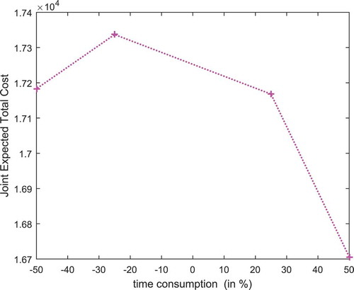
6 Sensitivity analysis

This section investigates how large variation of cost parameters impact the solution and total costs. There are some insights provided in the analysis which allow the manager to determine what decisions might be taken when one of the parameters change. The parameters $A$, $\pi$, $P$, $W_p^x$, $W_t^x$ and $t$ varied discretely from −50% to +50% of their base values. The results of the sensitivity analysis are presented in Table 3.

Table 3. Sensitivity analysis for different key parameters

	$\mathrm{\%}$	$JETC$		$\mathrm{\%}$	$JETC$
	$+50\mathrm{\%}$	18,478		$+50\mathrm{\%}$	15,902
$A$	$+25\mathrm{\%}$	15,914	$W_p^x$	$+25\mathrm{\%}$	15,891
	$-25\mathrm{\%}$	15,576		$-25\mathrm{\%}$	15,902
	$-50\mathrm{\%}$	15,394		$-50\mathrm{\%}$	15,910
	$+50\mathrm{\%}$	16,021		$+50\mathrm{\%}$	15,908
$\pi$	$+25\mathrm{\%}$	15,984	$W_t^x$	$+25\mathrm{\%}$	15,912
	$-25\mathrm{\%}$	15,870		$-25\mathrm{\%}$	15,917
	$-50\mathrm{\%}$	15,825		$-50\mathrm{\%}$	16,023
	$+50\mathrm{\%}$	16,706		$+50\mathrm{\%}$	16,706
$P$	$+25\mathrm{\%}$	16,293	$t$	$+25\mathrm{\%}$	17,168
	$-25\mathrm{\%}$	15,506		$-25\mathrm{\%}$	17,337
	$-50\mathrm{\%}$	15,158		$-50\mathrm{\%}$	17,183

Table 4. Outline of the algorithm for this problem

$g$	$p$	$m$	$q_1$	Actual capacity on dis.subs			Actual capacity on trans.subs			Actual capacity on power plant			$k_1$	$k_2$	$JETC$
				$W_d^y$	$\mathrm{C}\mathrm{o}\mathrm{n}\mathrm{c}\mathrm{l}\mathrm{u}\mathrm{s}\mathrm{i}\mathrm{o}\mathrm{n}$	$q_1$ revised	$W_t^y$	$\mathrm{C}\mathrm{o}\mathrm{n}\mathrm{c}\mathrm{l}\mathrm{u}\mathrm{s}\mathrm{i}\mathrm{o}\mathrm{n}$	$q_1$ revised	$W_p^y$	$\mathrm{C}\mathrm{o}\mathrm{n}\mathrm{c}\mathrm{l}\mathrm{u}\mathrm{s}\mathrm{i}\mathrm{o}\mathrm{n}$
1	1	1	103.8014	3114		103.8014	3114		103.8014	3114		103.8014	2.8115	0.9608	17,979
1	1	2	56.8224	1704.67		56.8224	1704.67		56.8224	3409.34		56.8224	2.8500	0.9210	15,875
1	3	3	41.5335	1246.01		41.5335	3738.02		41.5335	11,214.05		41.5335	2.7221	0.8625	15,606
1	4	4	34.1676	1025.028		34.1676	4100.11		34.1676	16,400.45		34.1676	2.5683	0.8059	15,728
1	3	5	29.5015	885.05		29.5015	2655.14		29.5015	13,275.68		29.5015	2.5631	0.7992	16,057

Table 5. The summary of results

Decision variables	Unit	Values
Electrical power distribution factor on the power plant	times	3
Electrical power distribution factor on the transmission substation	times	3
Electrical power distribution facotr on the distribution substation	times	1
Energy produced by the power plant (Ep = q1tgpm)	kWh	8971
Energy supplied by the transmission substation (Et = q1tgp)	kWh	2990
Energy supplied by the distribution substation (Ed = q1tg)	kWh	996.80
Actual power plant capacity	kVA	11,214
Actual transmission substation capacity	kVA	3738
Actual distribution substation capacity	kVA	1246

Table 6. Sensitivity analysis for different key parameters

Parameters	changes in %	JETC	Parameters	changes in %	JETC
	$+50\mathrm{\%}$	18,478		$+50\mathrm{\%}$	15,902
$A$	$+25\mathrm{\%}$	15,914	$W_p^x$	$+25\mathrm{\%}$	15,891
	$-25\mathrm{\%}$	15,576		$-25\mathrm{\%}$	15,902
	$-50\mathrm{\%}$	15,394		$-50\mathrm{\%}$	15,910
	$+50\mathrm{\%}$	16,021		$+50\mathrm{\%}$	15,908
$\pi$	$+25\mathrm{\%}$	15,984	$W_t^x$	$+25\mathrm{\%}$	15,912
	$-25\mathrm{\%}$	15,870		$-25\mathrm{\%}$	15,917
	$-50\mathrm{\%}$	15,825		$-50\mathrm{\%}$	16,023
	$+50\mathrm{\%}$	16,706		$+50\mathrm{\%}$	16,706
$P$	$+25\mathrm{\%}$	16,293	$t$	$+25\mathrm{\%}$	17,168
	$-25\mathrm{\%}$	15,506		$-25\mathrm{\%}$	17,337
	$-50\mathrm{\%}$	15,158		$-50\mathrm{\%}$	17,183

6.1 Managerial implications

1. Based on Table 3, it can be observed that $JETC$ is moderately sensitive to the change in ordering cost $A$ through a feasible range from −50% to +50%. It shows that $A$ has a moderate significant impact on the cost performance and the graphical representation is shown in Figure 1.

2. Through a feasible range (−50% to +50%), it can be seen that the $JETC$ is slightly sensitive to the change in $\pi$. The result in Table 3 is also presented in Figure 2.

3. From Table 3, it can be inferred that $JETC$ is slightly sensitive to the change in $P$ if the value of $P$ is increased. The result in Table 3 are depicted in Figure 3.

4. It can be observed, based on Table 3, that the $JETC$ is slightly sensitive to the change in maximum capacity of power plant and transmission substation. The result in Table 2 is also presented in Figures 4 and 5.

5. The time consumption is more effective for this model. Table 3 shows that the $JETC$ is highly sensitive to the change in $t$ and the graphical representation is shown in Figure 6. From this Table 3, it is clear that the time consumption is more sensitive for this model.

Figure 1. Change of parameter $A$ in total cost

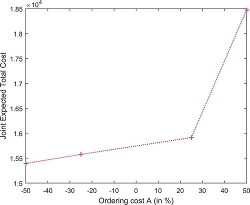
Figure 2. Change of parameter $\pi$ in total cost

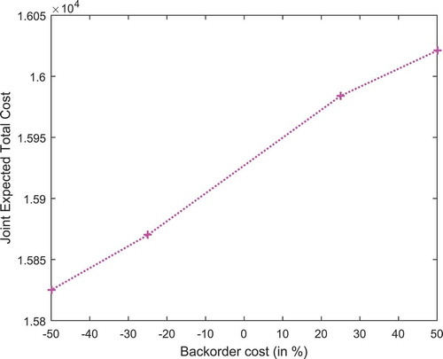
Figure 3. Change of parameter $P$ in total cost

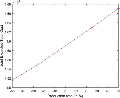
Figure 4. Change of parameter $W_p^x$ in total cost

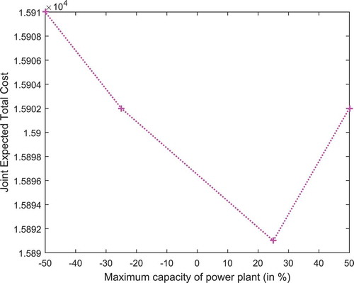
Figure 5. Change of parameter $W_t^x$ in total cost

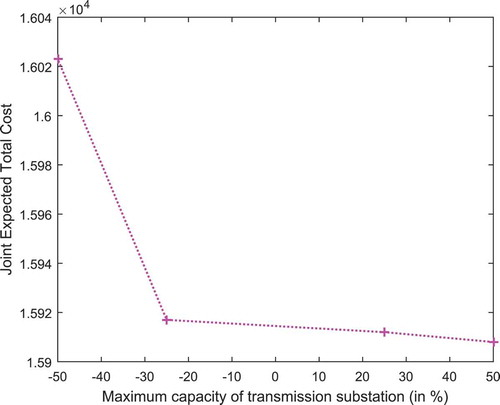
Figure 6. Change of parameter $t$ in total cost

7 Conclusion

This research developed an integrated inventory model where a single power plant produced an electricity and send it to the customer by transmission and distribution substations. In this model, we have considered a stochastic electricity demand, safety factors and two types of crashed lead time. We formulate a integrated total cost function which is mixed integer programming problem. Since the objective function is highly non-linear and all the decision variables are function of other decision variables. So we can’t find the closed loop form to get the optimal solutions. For this reason, we choose an iterative method to find the solution. The algorithmic procedure is developed for step by step iterative process (Table 4). Finally, this chapter conclude with numerical example (Table 5). Sensitivity analysis is performed for the different values of the parameters $A$, $\pi$, $P$, $W_p^x$, $W_t^x$ and $t$ (Table 6). The graphical interpretation of the sensitivity analysis are also presented. Managerial implications are also given according to the results of the sensitivity analysis. This work can be extended in several ways. One can consider lead time demand as a fuzzy random variable for future research. Further the proposed model can be extended to consider more realistic situations such as multi-echelon supply chains with single-buyer multiple vendors, multiple buyers and single vendor or multiple buyers and multiple vendors.

Disclosure statement

No potential conflict of interest was reported by the authors.

Additional information

Funding

The first author research work is supported by DST-INSPIRE Fellowship, Ministry of Science and Technology, Government of India under the grant no. DST/INSPIRE Fellowship/2014/IF170071 and UGC-SAP(DSA I), Department of Mathematics, The Gandhigram Rural Institute(Deemed to be University), Gandhigram-624302, Tamilnadu, India.

Notes on contributors

S. Hemapriya

S. Hemapriya is a Full Time Research Scholar in the Department of Mathemtics at The Gandhigram Rural Institute – Deemed University,  Gandhigram, India. He received his BSc in Mathematics from The Gandhigram Rural Institute – Deemed University, India in 2014 and MSc in Mathematics from The Gandhigram Rural Institute – Deemed University, India in 2016. His research interests include the following fields: operations research, inventory control, supply chain management. 

R. Uthayakumar

R. Uthayakumar is currently a Professor and the Head in the Department of Mathematics at The Gandhigram Rural Institute – Deemed University, Gandhigram, India. He received his MSc in Mathematics from the American College, Madurai, India in 1989 and PhD in Mathematics from The Gandhigram Rural Institute – Deemed University, Gandhigram, India in 2000.He has published about 80 papers in international and national journals. Hisresearch interests include the following fields: operations research, industrialengineering and fractal analysis.

References

- Annadurai, K., and R. Uthayakumar. 2010. “Reducing Lost-sales Rate in (T, R, L) Inventory Model with Controllable Lead Time.” Applied Mathematical Modelling 34: 3465–3477. doi:https://doi.org/10.1016/j.apm.2010.02.035.
- Ben-Daya, M. A., and A. Raouf. 1994. “Inventory Models Involving Lead Time as a Decision Variable.” Journal of the Operational Research Society 45 (5): 579–582. doi:https://doi.org/10.1057/jors.1994.85.
- Chen, C. K., H. C. Chang, and L. Y. Ouyang. 2001. “A Continuous Review Inventory Model with Ordering Cost Dependent on Lead Time.” International Journal of Information and Management Sciences 12: 1–13.
- Fossati, J. P., A. Galarza, A. Martín-Villate, and L. Fontan. 2015. “A Method for Optimal Sizing Energy Storage Systems for Microgrids.” Renewable Energy 77: 539–549. doi:https://doi.org/10.1016/j.renene.2014.12.039.
- Gallego, G., and I. Moon. 1993. “The Distribution Free Newsboy Problem: Review and Extensions.” Journal of the Operational Research Society 44 (8): 825–834. doi:https://doi.org/10.1057/jors.1993.141.
- Goyal, S. K. 1988. “A Joint Economic-lot-size Model for Purchaser and Vendor: A Comment.” Decision Sciences 19 (1): 236–241. doi:https://doi.org/10.1111/j.1540-5915.1988.tb00264.x.
- Goyal, S. K. 1995. “A One-vendor Multi-buyer Integrated Inventory Model: A Comment.” European Journal of Operational Research 82 (1): 209–210. doi:https://doi.org/10.1016/0377-2217(93)E0357-4.
- Goyal, S. K., and F. Nebebe. 2000. “Determination of Economic Production-shipment Policy for a Single-vendor-single-buyer System.” European Journal of Operational Research 121 (1): 175–178. doi:https://doi.org/10.1016/S0377-2217(99)00013-2.
- Hill, R. M. 1997. “The Single-vendor Single-buyer Integrated Production-inventory Model with a Generalized Policy.” European Journal of Operational Research 97 (3): 493–499. doi:https://doi.org/10.1016/S0377-2217(96)00267-6.
- Hoque, M. A., and S. K. Goyal. 2006. “A Heuristic Solution Procedure for an Integrated Inventory System under Controllable Lead-time with Equal or Unequal Sized Batch Shipments between A Vendor and A Buyer.” International Journal of Production Economics 102 (2): 217–225. doi:https://doi.org/10.1016/j.ijpe.2005.02.012.
- Liao, C. J., and C. H. Shyu. 1991. “An Analytical Determination of Lead Time with Normal Demand.” International Journal of Operations & Production Management 11 (9): 72–78. doi:https://doi.org/10.1108/EUM0000000001287.
- Luo, X., J. Wang, M. Dooner, and J. Clarke. 2015. “Overview of Current Development in Electrical Energy Storage Technologies and the Application Potential in Power System Operation.” Applied Energy 137: 511–536. doi:https://doi.org/10.1016/j.apenergy.2014.09.081.
- Ouedraogo, N. S. 2017. “Modeling Sustainable Long-term Electricity Supply-demand in Africa.” Applied Energy 190: 1047–1067. doi:https://doi.org/10.1016/j.apenergy.2016.12.162.
- Ouyang, L. Y., N. C. Yeh, and K. S. Wu. 1996. “Mixture Inventory Model with Backorders and Lost Sales for Variable Lead Time.” Journal of the Operational Research Society 47 (6): 829–832. doi:https://doi.org/10.1057/jors.1996.102.
- Pan, J. C. H., and J. S. Yang. 2002. “A Study of an Integrated Inventory with Controllable Lead Time.” International Journal of Production Research 40 (5): 1263–1273. doi:https://doi.org/10.1080/00207540110105680.
- Pandey, A., M. Masin, and V. Prabhu. 2007. “Adaptive Logistic Controller for Integrated Design of Distributed Supply Chains.” Journal of Manufacturing Systems 26 (2): 108–115. doi:https://doi.org/10.1016/j.jmsy.2007.11.001.
- Sarkar, B., R. Guchhait, M. Sarkar, S. Pareek, and N. Kim. 2019. “Impact of Safety Factors and Setup Time Reduction in a Two-echelon Supply Chain Management.” Robotics and Computer-Integrated Manufacturing 55: 250–258. doi:https://doi.org/10.1016/j.rcim.2018.05.001.
- Schneider, M., K. Biel, S. Pfaller, H. Schaede, H., . S. Rinderknecht, and C. H. Glock. 2016. “Using Inventory Models for Sizing Energy Storage Systems: An Interdisciplinary Approach.” Journal of Energy Storage 8: 339–348. doi:https://doi.org/10.1016/j.est.2016.02.009.
- Schneidera, M., K. Bielb, S. Pfallera, S., . H. Schaedea, S. Rinderknechta, and C. H. Glock. 2015. “Optimal Sizing of Electrical Energy Storage Systems Using Inventory Models.” Energy Procedia 73: 48–58. doi:https://doi.org/10.1016/j.egypro.2015.07.559.
- Taylor, J. A., J. L. Mathieu, D. S. Callaway, and K. Poolla. 2017. “Price and Capacity Competition in Balancing Markets with Energy Storage.” Energy Systems 8 (1): 169–197. doi:https://doi.org/10.1007/s12667-016-0193-9.
- Teng, J. T., L. E. Cárdenas-Barrón, and L. R. Lou. 2011. “The Economic Lot Size of the Integrated Vendor-buyer Inventory System Derived without Derivatives: A Simple Derivation.” Applied Mathematics and Computation 217 (12): 5972–5977. doi:https://doi.org/10.1016/j.amc.2010.12.018.
- Tsou, C. S., H. H. Fang, H. C. Lo, and C. H. Huang. 2009. “A Study of Cooperative Advertising in A Manufacturer-retailer Supply Chain.” International Journal of Information and Management Sciences 20 (1): 15–26.
- Uthayakumar, R., and M. Rameswari. 2012. “An Integrated Inventory Model for a Single Vendor and Single Buyer with Order-processing Cost Reduction and Process Mean.” International Journal of Production Research 50 (11): 2910–2924. doi:https://doi.org/10.1080/00207543.2011.575893.
- Wangsa, I., T. Yang, and H. Wee. 2018. “The Effect of Price-Dependent Demand on the Sustainable Electrical Energy Supply Chain.” Energies 11 (7): 16–45. doi:https://doi.org/10.3390/en11071645.
- Wangsa, I. D., and H. M. Wee. 2018. “The Economical Modeling of a Distribution System for Electricity Supply Chain.” Energy Systems 1–21.
- Wu, A., A. Philpott, and G. Zakeri. 2017. “Investment and Generation Optimization in Electricity Systems with Intermittent Supply.” Energy Systems 8 (1): 127–147. doi:https://doi.org/10.1007/s12667-016-0210-z.