A side-sampling based Linformer model for landslide susceptibility assessment: a case study of the railways in China

Abstract

The improvement of landslide susceptibility assessment is a long-standing problem in hazard mitigation work, wherein previous studies have proposed various training models. However, the ratio of positive to negative samples and the selection of non-landslide samples have been shown to significantly influence results. These research directions have traditionally been focal points, while datasets are often overlooked, serving merely as auxiliary tools to support the validation process. Hence, this study proposes an approach to enhance datasets through the introduction of the side-sampling method. This technique focuses on individual research cells, conducting feature sampling training on fixed regions of length M, thereby enabling more precise identification of geographical clustering characteristics. Using evaluation metrics such as accuracy, precision, recall, F1 score, and ROC curve, this study conducts a comparative analysis between the side-sampling method and traditional sampling methods, using three distinct railway lines in China as the study areas. Results show substantial improvements beyond several exceptions: accuracy (+7.68%), precision (+7.19%), recall (+13.48%), F1 score (+9.92%), and ROC (+6.22%). The results demonstrate a significant overall improvement in the performance of the trained models based on the side-sampling method, providing a positive insight into mitigating landslide hazards along railways from the dataset perspective.

Keywords:

• Landslide
• susceptibility assessment
• railway hazard
• side-sampling
• Linformer model

1. Introduction

The railway plays a pivotal role in supporting economic development (Chi and Han 2023). Railways involve extensive linear engineering, crossing various regions, making them susceptible to natural hazards. Disruptions caused by these hazards can lead to significant economic losses and societal impacts. Landslides, as the second most common natural disaster, involve the downhill movement of mountainous materials along a sliding surface under the influence of gravity. Their wide distribution and destructive characteristics have a significant impact on railways that cannot be overlooked (Yong and Peijun 2008; Yan et al. 2020; Azarafza et al. 2021). Consequently, the identification of landslide-prone areas and risk management has become a key focus of landslide hazard research, with landslide susceptibility assessment being an effective technique of investigation (Guzzetti et al. 2006; Reichenbach et al. 2018; Fu et al. 2023). Landslide susceptibility mapping (LSM) involves the evaluation and grading of regional spatial landslide probabilities through the analysis of geological, geomorphological and hydrological factors, as well as data from landslide inventories (Liu et al. 2023). Such a methodical evaluation provides decision-makers with a scientific and effective basis for hazard prevention, early warning, planning, design, and risk mitigation (Lin et al. 2021; Huang et al. 2022).

Landslide susceptibility assessment is a complex task that requires both challenging data acquisition and the appropriate application of analytical techniques (Akgun et al. 2008; Nikoobakht et al. 2022). In order to overcome the limitations inherent in current research, and to promote enhancements in accuracy and credibility, scholars in recent years have predominantly focused on the refinement of algorithmic models, exploration of relationships between positive and negative samples, and scientific non-landslide sample selection methods development (Reichenbach et al. 2018; M. Liu et al. 2021; Ghorbanzadeh et al. 2022).

The literature review indicates that Bhagya et al. 2023 multi-criteria decision analysis model (Bahrami et al. 2021), statistical models (Sonker et al. 2022), and machine learning models (Ado et al. 2022) have been successfully employed to simulate the complex relationships between landslides and conditioning factors. Given the extensive application of the AHP and fuzzy-AHP models in LSM studies, they are frequently used to compare against other research methodologies to forecast potential landslide events (Agrawal and Dixit 2022; Bhagya et al. 2023). The sensitivity of SVM, LR, and ANN models to training datasets has been analyzed under scenarios involving five randomly sampled training datasets (Kalantar et al. 2018). However, as the performance of traditional models gradually becomes inadequate, numerous studies have turned to the optimization and compensation through hybrid and ensemble techniques, yielding results that are more accurate and reliable. For instance, Pham et al. (2019) combined sequential minimal optimization and support vector machine models to simplify the algorithm and reduce complexity. Kavzoglu and Teke (2022) employed XGBoost for efficient supervised classification, mitigating overfitting through bagging-bootstrap. Furthermore, deep learning methods (LeCun et al. 2015), including CNN (Youssef et al. 2022), RNN (Yi et al. 2022), and LSTM (Hamedi et al. 2022) have been widely used. Li et al. 2023 Jiang et al. 2023, Furthermore, developing and improving deep learning models from various perspectives has significantly enhanced their ability to recognize landslides. For instance, CNN-2D has proven to be a more reliable modeling technique than SVM and CNN-1D (Youssef et al. 2022). Optimization of sample patches has led to an approximate 3% increase in mIOU values for trustworthy CNN algorithms (Ghorbanzadeh and Blaschke 2019). Using the traditional ResNet algorithm as a base, combined with LSTM and GoogLeNet in an ensemble deep learning algorithm, has improved the prediction of landslides in terms of AUC and accuracy by 3%–4% and 2%, respectively, compared to conventional models (Li et al. 2023). The combination of InSAR technology with deep learning models has been demonstrated to be effective. Specifically, the FCADenseNet model, which integrates an attention mechanism, has shown a positive impact on the recognition of landslides (Li et al. 2024). Additionally, research has introduced a novel lightweight deep learning model, MS2LandsNet, which significantly reduces parameter count and overall complexity through architectural adjustments, demonstrating superior performance compared to both classical deep learning and lightweight models (Lu et al. 2024). Furthermore, Ghorbanzadeh has showcased various innovative deep learning models, such as the Swin Transformer, SegFormer, and U-Net, achieving more accurate and timely landslide detection (Ghorbanzadeh et al. 2022).

One prevalent challenge in landslide susceptibility assessment research is the imbalance between non-landslide and landslide samples, which can significantly impact model performance (Wang et al. 2019). Studies have shown that the ratio of landslide to non-landslide samples is crucial for building effective prediction models (Shao et al. 2020; Zhou et al. 2021). Over-reliance on landslide data can lead to susceptibility overfitting, while excessive use of non-landslide data may result in data contamination and reduced performance (Gao et al. 2020; Yang et al. 2023). One perspective suggests that when the balance between positive and negative sample ratios shifts from equilibrium to imbalance, the corresponding sensitivity values exhibit more noticeable fluctuations (Zhuo et al. 2023). Studies employing multiple models based on varying numbers of conditioning factors have been conducted, and the results indicate that the optimal ratio is between 1.5 and 2 (Zhao et al. 2020). In addition, Pourghasemi et al. (2020) and Nam et al. (Nam and Wang 2019) share the same perspective in their research, highlighting that the model’s performance is significantly compromised when there is a notable difference in the proportion of negative and positive samples.

In prior research, the selection method for non-landslide samples has been demonstrated as an effective approach to enhance the assessment of landslide susceptibility. In comparison to the common random sampling within the region (Al-Najjar et al. 2021), the selection method for non-landslide samples based on river and slope conditions (Kavzoglu et al. 2014) and the buffer zones outside landslide areas (Nefeslioglu et al. 2008) is considered more reliable. Given that the criteria for selecting non-landslide samples are determined by the researchers, these methods are considered subjective. To address the randomness associated with non-landslide data selection, techniques like subsampling (Yang et al. 2022), the Synthetic Minority Oversampling Technique (SMOTE) (Agrawal et al. 2017), and Easysemble (Al-Najjar et al. 2021) have been developed to improve the reliability of non-landslide data and enhance model accuracy.

Given the above research, scholars have conducted in-depth studies on model algorithms, the ratio of landslide to non-landslide quantities, and the selection of non-landslide samples. However, datasets containing rich information are often overlooked. Despite supplementing landslide inventories in regions with insufficient representation in the literature through image-based landslide data, the receiver operating characteristic (ROC) did not show significant differences due to the more uniformly distributed and enriched data (Broeckx et al. 2018). Based on oversampling techniques, the augmentation of landslide data was compared with the original data across three different sample sizes. While there has been some improvement in performance, the overall outcome showed a lack of consistency (Gao et al. 2020). Additionally, transforming original data into high-trust landslide and non-landslide data using a semi-supervised learning framework altered the dataset (Zhang and Yan 2022). While the accuracy of model predictions improved, a significant portion of high-trust non-landslide points, mostly associated with water bodies, and the characteristics of overfitting caused by clustering algorithms, made it challenging to generalize on a large scale.

According to above-mentioned research, it appears that the supplementation of a uniformly distributed landslide did not show significant effects, perhaps due to the large size of the training sample set. However, methods involving sample augmentation and geographic clustering characteristics exhibit potential for model optimization. Therefore, an approach considering the advantages of both methods could provide a new perspective on landslide susceptibility.

Addressing the above issues, this study aims to investigate landslide susceptibility from the perspectives of sample augmentation and geographic clustering characteristics. Drawing on the strong spatial correlation exhibited by landslide occurrences in specific regions with similar features (Chang et al. 2023), this paper proposes a side-sampling method. This approach focuses on the geographical proximity between study units and their surrounding units, emphasizing the capture of rich information from the surrounding units to reveal similar features. Using three railways in China as a case study, the side-sampling method is explained and analyzed based on multiple models.

2. Method

2.1. Procedure of LSM based on side-sampling method

The flowchart of this study is illustrated in Figure 1, and the main steps include:

Figure 1. The flowchart of a side-sampling method for landslide susceptibility assessment.

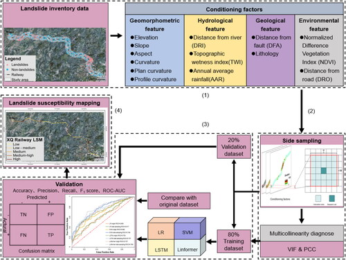
1. Preparation of landslide inventory and base data: The study area is determined, and landslide inventories are established based on different data sources within the study area, generating an equivalent number of negative samples. Fundamental geological, hydrological, environmental, and geomorphological data within the study area are collected. Existing data resolutions are matched, and the raw data is converted into raster layers.

2. Acquisition of conditioning factors within fixed area and verification of multicollinearity: Using the research cell as the center, neighborhood units within fixed areas are selected as cell data for the side-sampling method. Conditioning factors within fixed areas are extracted as basic input data, including geological, hydrological, environmental, and geomorphological factors. Multicollinearity diagnosis is performed using Variance Inflation Factor (VIF) and Pearson’s Correlation Coefficient (PCC).

3. Validation of model performance under the side-sampling method and traditional method: The logistic regression (LR), support vector machine (SVM), long short-term memory (LSTM), and Linformer models are applied for landslide susceptibility assessment based on the side-sampling method. Using the same research cells, traditional sampling methods are employed for different models landslide susceptibility assessment. Confusion matrices and ROC curves are used to compare the model performance between the two sampling methods.

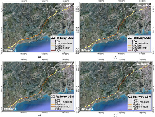
4. Consistency test for railway landslide susceptibility: Based on the side-sampling method, landslide susceptibility results for the three railways within the study area are calculated. The evaluation results are plotted on LSM of various models to validate the consistency of potential landslide occurrences. The LSM is divided into five levels (low, low-medium, medium, medium-high, high).

2.2. Model algorithm

In this study, four distinct algorithms were employed as the foundation for comparing the impacts of the side-sampling data collection method and the traditional sampling method on landslide susceptibility evaluation. These algorithms include LR, SVM, LSTM, and Linformer, encompassing both classical statistical and modern machine learning and deep learning methods (R. Liu et al. 2021; Habumugisha et al. 2022). Linformer, in particular, represents a novel deep learning approach (Jiang et al. 2023). By comparing these diverse algorithms, we aim to comprehensively illustrate the applicability of the side-sampling method, ensuring the robustness and credibility of the results.

2.2.1. Logistic regression

Logistic regression, a classical multivariate statistical method, is widely acknowledged for its reliability in geohazard analysis research. The logistic function based on the LR method distributes the resultant values between 0 and 1, estimating the probability of hazard occurrence through maximum likelihood estimation rather than directly predicting hazard existence. This makes LR well-suited for landslide susceptibility analysis (King and Zeng 2003; Brenning 2005; Xi et al. 2022).

2.2.2. SVM

SVM is a supervised classification machine learning algorithm rooted in statistical learning theory, which is good at solving regression analysis and multifaceted classifier problems, making it particularly useful in various hazard prediction and analysis research, including landslide susceptibility assessment (Huang and Zhao 2018; Akinci and Zeybek 2021; Saha et al. 2022). This method is able to cope with the processing of complex data, flexibly avoiding the noise problem and ensuring high generalization capability (Dang et al. 2020).

2.2.3. LSTM

LSTM is an optimized algorithm within the realm of recurrent neural networks (RNNs). The uniqueness of the LSTM model lies in its capacity to control the information flow through a specialized ‘memory block’ gating mechanism. This mechanism enables the LSTM model to selectively acquire knowledge from the hidden layer cell using three distinct gating units: the forget gate, input gate, and output gate. These gating units collectively determine whether to retain or discard the incoming data (Kim and Kim 2020; Xu et al. 2022). Capitalizing on its ability for long-term and short-term memory, wherein it assigns weights and learns cell states, LSTM surpasses conventional RNN models by exhibiting learning ability in long-term dependency (Hamedi et al. 2022).

2.2.4. Linformer

The Transformer model has demonstrated its versatility by effectively addressing a wide array of problems and finding extensive application in domains like medicine and linguistics (Kalyan et al. 2022; He et al. 2023). Furthermore, a growing number of scholars have recognized its potential utility in the realm of geological hazard research (Bao et al. 2022). However, despite its remarkable self-attention mechanism, this model still presents certain limitations in practical applications, notably in terms of its slow training speed and high training costs. In response to these challenges, researchers have introduced the Linformer model. Linformer model avoids quadratic operations by reducing the complexity of sequence length in training from O(n²) to O(n). This transformation is achieved through the fragmentation of the original scaled dot-product attention into multiple smaller components via linear projection. Additionally, the Linformer model dissects the original attention into low-rank factors, contributing to its enhanced computational efficiency (S. Wang et al. 2020).

A rendering of Linformer’s self-attention mechanism is shown below: (1) $$\begin{array}{c}\overline{{\mathit{\text{head}}}_i}=\mathit{\text{Attention}}\left(Q{W}_i^Q,E_{i}K{W}_i^K,F_{i}V{W}_i^V\right)\\ =\underset{{\overline{P}:}_{n\times k}}{\underbrace{\mathit{\text{softmax}}\left[\frac{Q{W}_i^Q{\left(E_{i}K{W}_i^K\right)}^T}{\sqrt{d_k}}\right]}}{F}_{i}V{W}_i^V\end{array}$$(1)

Where $W_i^Q,W_i^K,{\mathit{\text{and}} W}_i^V$ are the matrices to be trained and $Q,K,V$ are scaled using the key of dimension $d_k$ and the value of dimension $d_v$ for canceling out the effect of dot product. $K{W}_i^K$ and $V{W}_i^V$ are projected to the matrix and $E_i$ and $F_i$ are computed by scaling the dot product attention. Calculate the dot product of the query with all keys, divide it by $\sqrt{d_k},$ apply the softmax function to obtain the weight of the value, and finally calculate its dot product with all values (Vaswani et al. 2017). (2) $$\mathit{\text{MultiHead}}\left(Q,K,V\right)=\mathit{\text{Concat}}({\mathit{\text{head}}}_1,{\mathit{\text{head}}}_2,{\mathit{\text{head}}}_3,\dots ,{\mathit{\text{head}}}_n)$$(2)

The queries, keys and values differ between each $\mathit{\text{head}}$ and self-learn self-attention values. Subsequently, each value is multiplied with the weight matrix $W^O$ and output as shown in Equation (7)(7) $$\mathit{\text{Recall}}=\mathit{\text{TPR}}=\frac{\mathit{\text{TP}}}{\mathit{\text{TP}}+\mathit{\text{FN}}}$$(7) .

2.3. Side-sampling

The range and variation of regional-scale features and spatial granularity have significant impacts in ecology, where inappropriate analysis scale settings can often lead to unsatisfied accuracy due to variations in the study area’s scope (Wu 2004; Markham et al. 2023; Wang et al. 2023). In landscape ecology research, scholars have employed the moving-window method, recalculating index weights for multiple overlapping regions with a single pixel as the center within the study area and a radius of N (Zhu et al. 2020; 2021). This approach enhances accuracy by making full use of geographic proximity, and the redistribution of weights among multiple pixels ensures more realistic results (Riitters 2019; Zhu et al. 2020).

Inspired by this, the present study proposes a side-sampling dataset collection method based on data augmentation and geographic clustering characteristics. Unlike the previous moving-window technique, which segments a single pixel representing the study area into multiple equi-sized pixels for weighted feature calculation, our side-sampling method adopts a strategy with a higher potential for learning. It focuses on a single research cell and extends outward to a fixed area of length M, thereby collecting information within an M*M area and further mapping this information to the location of the subject cell. Figure 2 clearly illustrates the sample data collection process within the study area using the side-sampling method. As the value of M increases, both the captured geographic neighborhood and the features within this range undergo corresponding changes. If the value of M is sufficiently large, the two sample points may even partially extract overlapping adjacent cells.

Figure 2. Diagrammatic sketch of the side-sampling method.

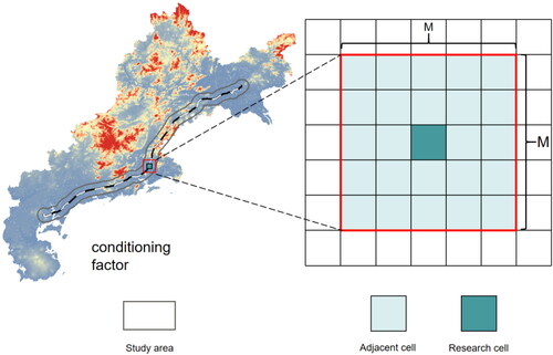
Although both the moving-window and side-sampling methods involve a transformation from single to multiple pixels, the moving window method primarily focuses on refining existing data to obtain more precise results. In contrast, the side-sampling method, recognizing the geographical clustering attributes between adjacent cells and the research cell, expands the research scope to explore underutilized neighborhood unit data. This approach adheres to the principles of the first law of geography (Tobler 1970), which posits that ‘Everything is related to everything else, but proximal things are more related to each other.’ This implies that cells with similar geographical features exhibit higher correlation, and by considering the influence of adjacent cells, it is possible to more accurately capture and reflect their characteristics (Lv et al. 2017).

2.4. Modeling validation

The quality of feature selection often has a considerable impact on landslide susceptibility assessment, and high correlation between factors can lead to low performance and time-consuming models, which in turn leads to unsatisfactory training results (Merghadi et al. 2018; Huang et al. 2023). To address this issue, VIF and PCC tests are valuable tools. Smaller VIF values indicate insignificant multicollinearity, while larger VIF implies strong multifactor intercollinearity. Researchers often use a VIF value exceeding 5 or 10 as an indicator of multicollinearity in their studies. To ensure the accuracy of this study, a threshold of 5 was employed to identify multicollinearity (Merghadi et al. 2020). The VIF value is calculated as follows: (3) $$\mathit{\text{VIF}}=\frac{1}{1-R_i^2}$$(3)

Where $R_i$ is the negative correlation coefficient of the independent variable x analyzed in a regression analysis on the remaining independent variables, and $1-R_i^2$ denotes tolerance. The correlation between any two conditioning factors was calculated by PCC with the following equation: (4) $$r\left(X,Y\right)=\frac{\mathit{\text{Cov}}(X,Y)}{\sqrt{\mathit{\text{Var}}\left|X\right|\mathit{\text{Var}}\left|Y\right|}}$$(4)

Where $\mathit{\text{Cov}}(X,Y)$ is the covariance of $X$ and $Y,$ $\mathit{\text{Var}}\left|X\right|$ is the variance of $X,$ and $\mathit{\text{Var}}\left|Y\right|$ is the variance of $Y.$ Typically, whether the PCC exceeds 0.7 is taken as a criterion for verifying high correlation (Avand et al. 2020).

2.5. Model performance evaluation

Landslide susceptibility evaluation is a serious scientific endeavour that requires different metric tools to judge model performance. Accuracy, precision, recall and F₁ score are crucial indicators for assessing the training model and serve as valuable measurement tools (Merghadi et al. 2018; Yu et al. 2021). The accuracy (Equation 5(5) $$\mathit{\text{Accuracy}}=\frac{\mathit{\text{TP}}+\mathit{\text{TN}}}{\mathit{\text{TP}}+\mathit{\text{FP}}+\mathit{\text{TN}}+\mathit{\text{FN}}}$$(5) ), serving as a fundamental metric for assessing the overall predictive correctness of the model, reflects the model’s capability in distinguishing areas susceptible to landslides from non-susceptible areas. However, relying solely on accuracy may overlook the model’s performance in specific classifications. Therefore, the introduction of precision (Equation 6(6) $$\mathit{\text{Precision}}=\frac{\mathit{\text{TP}}}{\mathit{\text{TP}}+\mathit{\text{FP}}}$$(6) ) and recall (Equation 7(7) $$\mathit{\text{Recall}}=\mathit{\text{TPR}}=\frac{\mathit{\text{TP}}}{\mathit{\text{TP}}+\mathit{\text{FN}}}$$(7) ) as complementary metrics addresses, respectively, the ability to identify landslide areas with low false positive rates and the capability to capture actual landslide areas. The F1 score (Equation 8(8) $$F_1\mathrm{ }\mathit{\text{score}}=2\times \frac{\mathit{\text{Precision}}\times \mathit{\text{Recall}}}{\mathit{\text{TPrecision}}+\mathit{\text{Recall}}}$$(8) ), as the harmonic mean of precision and recall, provides a comprehensive assessment, aiding in balancing false alarms and misses, ensuring efficient identification and classification of landslide susceptibility by the model.

Their values can be calculated based on the true positive (TP), true negative (TN), false positive (FP), and false negative (FN) value obtained from the confusion matrix (Sahin et al. 2020). In this context, TP and TN predict the number of correctly judged landslides and non-landslides, while FP and FN represent signify the number of misclassified landslides and non-landslides. These important metrics are close to 1 for good performance and 0 for poor results.

The receiver operating characteristic (ROC) curve is a frequently used metric to evaluate model robustness due to its ability to accurately predict the probability of events that have not yet been characterized (Tsangaratos and Ilia 2016). The value of the ROC curve varies between 0 and 1, with values closer to 1 indicating better predictive capabilities for landslides or non-landslides. The X and Y axes of the coordinates represent the false positive rate (FPR) and true positive rate (TPR), respectively, denoting the ratio of misclassified areas to the total number of non-landslides and the ratio of correctly classified areas to the total number of landslides (Zabihi et al., 2018; Satarzadeh et al., 2022). These rates can be deduced from Equations (7)(7) $$\mathit{\text{Recall}}=\mathit{\text{TPR}}=\frac{\mathit{\text{TP}}}{\mathit{\text{TP}}+\mathit{\text{FN}}}$$(7) and (9)(9) $$\mathit{\text{FPR}}=\frac{\mathit{\text{FP}}}{\mathit{\text{TN}}+\mathit{\text{FP}}}$$(9) . (5) $$\mathit{\text{Accuracy}}=\frac{\mathit{\text{TP}}+\mathit{\text{TN}}}{\mathit{\text{TP}}+\mathit{\text{FP}}+\mathit{\text{TN}}+\mathit{\text{FN}}}$$(5) (6) $$\mathit{\text{Precision}}=\frac{\mathit{\text{TP}}}{\mathit{\text{TP}}+\mathit{\text{FP}}}$$(6) (7) $$\mathit{\text{Recall}}=\mathit{\text{TPR}}=\frac{\mathit{\text{TP}}}{\mathit{\text{TP}}+\mathit{\text{FN}}}$$(7) (8) $$F_1\mathrm{ }\mathit{\text{score}}=2\times \frac{\mathit{\text{Precision}}\times \mathit{\text{Recall}}}{\mathit{\text{TPrecision}}+\mathit{\text{Recall}}}$$(8) (9) $$\mathit{\text{FPR}}=\frac{\mathit{\text{FP}}}{\mathit{\text{TN}}+\mathit{\text{FP}}}$$(9)

3. Case study

3.1. Study areas

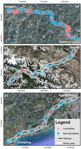
To access the universality of the side-sampling method, this study selected three railway lines located in different regions of China, as shown in Figure 3. The Xingquan railway (XQ railway) spans over 440 km, connecting south-central Jiangxi Province and southwestern Fujian regions, and serves as a main transportation from Quanzhou Port on the southeast coast to inland areas, with a bridge-to-tunnel ratio of more than 54%. The study area is situated in the southeastern edge of the Asia-Europe continental plate, adjacent to the east of the Pacific plate, with frequent crustal movements (Cao et al. 2020). Influenced by tectonic fractures, the geological strata and rock distribution exhibit a pattern of gradually rejuvenating from north to south and from west to east, forming a structural configuration known as the ‘east-west zone and north-south block’. The line passes through three distinct geomorphological units: tectonically eroded middle and low mountain ranges tectonically eroded low mountains and hills, and coastal plains and platform areas. Along the line belongs to the subtropical latitude range, with the characteristics of oceanic like continental transition. Due to the natural barrier effect of the two mountain ranges, mitigating the intrusion of cold air masses from the northwest and north during the winter months. Year-round rainfall distribution is more balanced, the average annual rainfall ranging from 1300 to 1800 mm. Furthermore, the region experiences minimal temperature fluctuations, maintaining a temperature range of 10 °C–29 °C.

Figure 3. Geo-graphical location map of the three study areas.

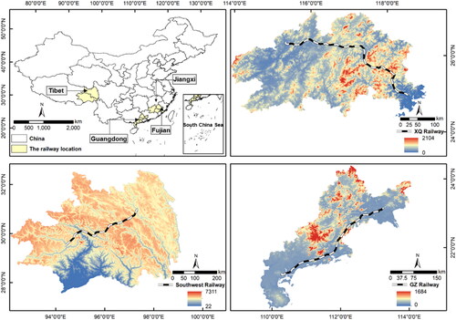
The southwest railway is situated in the eastern region of Tibet, China, and is subject to the influence of warm and humid air masses originating from the Pacific Ocean and the Indian Ocean. This railway is over 380 km and exhibits pronounced climatic variations, characterized by four distinct seasons, significant diurnal temperature fluctuations, and notable freeze-thaw weathering conditions. These conditions make the rock formations in the area susceptible to reduced stability (Zhang et al. 2021; Wang et al. 2022). At the same time, the region features a diverse topography marked by high mountains and valleys, with a noticeable elevation gradient from west to east (Peng et al. 2020). The geological structures along the route are diverse and the distribution of fault zones is dense, providing conditions for rainwater infiltration (Zeng et al. 2020). The average annual precipitation in this area falls within the range of 500–700 mm, with a sharp increase in both precipitation frequency and amount during the summer months, which can trigger landslide hazards within a short period of time (Qiao et al. 2019; Wang Shijin et al. 2021). The confluence of these multiple factors creates advantage for the occurrence of landslides.

The Guangzhan railway (GZ railway) extends for nearly 400 km and is oriented approximately from northeast (113.25°, 23.16°) to southwest (110.27°, 21.20°), traversing the Pearl River Delta region. The topography in this area is characterized by gentle terrain and is primarily categorized into three landform types: alluvial plains, middle and low mountainous areas, and denuded hilly areas. The study area belongs to the Yunkai Massif and the Yuezhong Massif, where frequent tectonic activities, predominantly vertical uplift and subsidence, coupled with local horizontal torsional movements, are observed. The region experiences intensive human engineering activities, resulting in a significant impact on the geological environment. The geological composition along the railway line is highly diverse, with substantial variations in lithofacies and engineering properties of rock and soil formations. The railway corridor falls within the subtropical oceanic monsoon climate zone, characterized by year-round moisture and warmth. It receives abundant rainfall, with average annual rainfall ranging from 1500 to 2300 mm. The flood season typically spans from April to September, during which period rainfall accounts for a substantial 82% of the total annual rainfall, thereby increasing the likelihood of landslide occurrences (Zhuo et al. 2023). Furthermore, the presence of densely distributed bedrock joints and fissures with low shear strength, coupled with hydrodynamic pressure from groundwater, often triggers shallow landslides, serving as favorable factors contributing to landslide hazards.

3.2. Datasets

In this study, 10 km we selected a 10 km-wide corridor along each railway line as the study area for landslide susceptibility assessment. It is well known that the proportion of landslide and non-landslide areas is significantly different, and it is unusually large even within the study area (Xu et al. 2022). To address this issue and ensure fairness in model training, the study randomly generates an equal number of non-landslide hazard sites corresponding to the number of landslide hazard sites (W.D. Wang et al. 2020), as illustrated in Figure 4.

Figure 4. Landslide inventories distribution in the study area: (a) XQ railway; (b) the southwest railway; (c) GZ railway.

In addition to the diversity in study areas, the utilization of various sources of landslide inventory data strengthens the verification of the universality of the side-sampling method. The landslide data for the southwest railway were obtained from China Railway First Survey and Design Institute Group Co., Ltd., while the landslide data for GZ Railway and XQ Railway were sourced from the Geographic Remote Sensing Ecological Network platform (http://www.gisrs.cn). The DEM was acquired from the Advanced Spaceborne Thermal Emission and Reflection Radiometer Global Digital Elevation Model (ASTER GDEM V3), which was jointly developed by NASA and JAXA. ASTER GDEM V3). Landsat 8 OLI remote sensing image were obtained from Geospatial data cloud (http://www.gscloud.cn), and 1:1,000,000 original engineering geological map were sourced from Geoscientific Data & Discovery Publishing System (http://dcc.cgs.gov.cn/). In addition, all conditioning factors were vectorised and rasterised into 30 × 30 m raster layers, matching the resolution of the DEM and Landsat 8 OLI data closely.

3.3. Conditioning factors

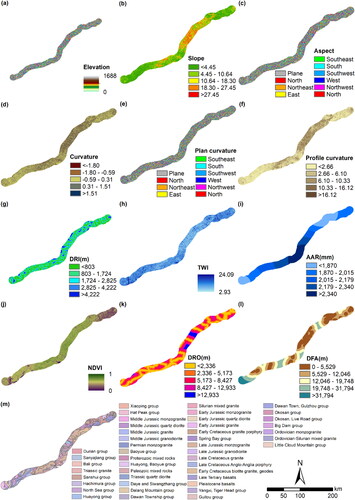
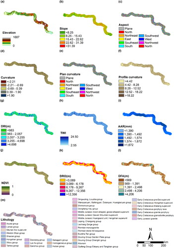
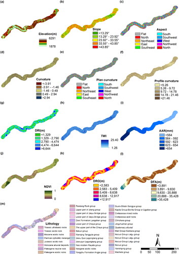
The selection of appropriate conditioning factors is a crucial aspect of landslide susceptibility assessment and forms the cornerstone of this analysis (Agrawal and Dixit 2022). However, no formal systematic procedure or agreement exists for the selection of conditioning factors (Ayalew and Yamagishi 2005). This study recommends to select the conditioning factors by the method of hazard types and available data (Dou et al. 2020). For our study, as depicted in Table 1, we employed the same set of 13 conditioning factors for all three railway lines, including geological features (elevation, slope, aspect, curvature, plane curvature, and profile curvature), hydrological features (DRI, TWI, and AAR), environmental features (NDVI, DRO), and geomorphological features (DFA, lithology). Further details about these conditioning factors are available in Appendices 1–3.

Table 1. Predictive performance of model testing dataset.

Railway	Indicators	Original				Side-sampling
		LR	SVM	LSTM	Linformer	LR	SVM	LSTM	Linformer
XQ railway	Accuracy	0.564	0.629	0.654	0.667	0.573	0.667	0.688	0.726
	Precision	0.561	0.650	0.647	0.671	0.571	0.663	0.699	0.735
	Recall	0.596	0.565	0.683	0.658	0.602	0.683	0.665	0.708
	F1 Score	0.578	0.605	0.665	0.665	0.586	0.673	0.682	0.722
Southwest railway	Accuracy	0.676	0.706	0.706	0.735	0.735	0.735	0.794	0.824
	Precision	0.800	0.818	0.818	0.900	0.833	0.833	0.917	0.789
	Recall	0.471	0.529	0.529	0.529	0.588	0.588	0.647	0.882
	F1 Score	0.593	0.643	0.643	0.667	0.690	0.690	0.759	0.833
GZ railway	Accuracy	0.689	0.711	0.711	0.711	0.711	0.733	0.778	0.822
	Precision	0.654	0.645	0.645	0.655	0.667	0.667	0.731	0.792
	Recall	0.773	0.909	0.909	0.864	0.818	0.909	0.864	0.864
	F1 Score	0.708	0.755	0.755	0.745	0.735	0.733	0.792	0.826

3.3.1. Elevation

Elevation is one of the most significant factors influencing the occurrence of landslides, and different elevations affect the change of slope, type of geotechnical body, and the degree of vegetation cover, which in turn affects the stability of slopes (Feizizadeh et al. 2014).

3.3.2. Slope

Slope is one of the factors that affect stability. The greater the slope, the more unfavorable the shear force will be in the balance between the soil sliding force and the shear force. At the same time, the change of slope has a significant effect on the soil saturation of the terrain surface (Sameen et al. 2020).

3.3.3. Aspect

Aspect is inextricably linked to sun radiation, rainfall, and vegetation cover, which is another factor associated with landslides (Nami et al. 2018). In the figure, there are nine types of slope orientations: eastern, southern, western, northern, northwestern, southwestern, northeastern, southeastern, and flat.

3.3.4. Curvature

Curvature represents changes in terrain surface slope, which influences the direction and velocity of slump body movement during landslide hazards (Zhao et al. 2022).

3.3.5. Plan curvature and profile curvature

Plan curvature and profile curvature are curvatures in the direction of slope direction and slope gradient, respectively, representing lateral or upward bulges and depressions at the unit (Moore et al. 1991; Florinsky 1998). Plan curvature plays a key role in the convergence and divergence of airflow, and profile curvature affects the acceleration or deceleration of water flow.

3.3.6. DRI

There is a correlation with the distance from the river (DRI) and the occurrence of landslides, and the amount of moisture within the soil affects the shear strength and thus the slope stability (Erener et al. 2017).

3.3.7. TWI

Topographic wetness index (TWI) is the embodiment of topographic features on the spatial distribution of soil moisture, reflecting the slope flow (Abedini et al. 2019). TWI in this study was classified according to five categories.

3.3.8. AAR

Annual average rainfall (AAR) is widely used in landslide susceptibility studies, which is unfavourable to slope stability (Rong et al. 2020). In this study, AAR data were calculated by interpolating rainfall sites near the study area.

3.3.9. NDVI

Normalized difference vegetation index (NDVI) provides a clear view of the distribution of vegetation, which can positively influence slope instability in soil and rock in the present time of increasing human activities (Bourenane et al. 2015). Its distribution ranges from −1 to 1 and is averaged into five classes according to the values.

3.3.10. DRO

The construction of roads encompasses excavation and rehabilitation, which will inevitably damage the original soil structure, leading to a decrease in slope stability, and is an important anthropogenic destructive factor (Chen and Fan 2023). The distance from the road (DRO) reflects its impact on landslides.

3.3.11. DFA

Faults have a difficult to ignore the role of the development of terrain structure, reducing the strength of the rocks along the fault, steepening the probability of landslide disaster (Binh Thai Pham et al. 2015). In this article, the distance from the fault (DFA) is divided into different regions through Euclidean distance.

3.3.12. Lithology

The physical and geomechanical characteristics of lithology are very different under the tectonic action of different ages, and the cohesion and internal friction angle will have non-negligible differences, so it is necessary to divide the area according to different lithological ages (Shao and Xu 2022). The study area is complex with numerous lithological types.

3.4. Preparation of the sample datasets and diagnosis of multicollinearity

To accurately delineate landslide susceptibility zones, this study emphasizes the significance of both an appropriate training model and the datasets containing conditioning factors and historical landslide occurrence information. In this research, a fixed area of M = 3, representing the neighborhood units encircling the study unit, was adopted for the side-sampling method. While there is no universally accepted standard or rule of thumb for the training set-to-test set ratio, this study employs an 80/20 ratio based on the dataset’s size. Specifically, the XQ railway boasts a larger historical landslide dataset with 801 instances, whereas the southwest railway and the GZ railway have fewer landslides, with 85 and 112 occurrences, respectively. Training samples with a balanced ratio perform better than those with a high imbalance ratio (Weiss and Provost 2003). Therefore, an equal number of non-landslide data are selected for both the training and validation sets. During model training, the labeled outcomes are composed of landslide data with a label value of 1 and non-landslide data with a label value of 0. Furthermore, the randomly selected non-landslide samples are not contained within the M*M fixed region allocated for landslide samples according to the side-sampling method. Additionally, 13 conditioning factors include geological, hydrological, environmental, and geomorphological features were selected for landslide susceptibility assessment.

It is noteworthy that the training samples for the model were constructed by randomly selecting 80% of proportional samples from the dataset, which were then expanded through the side-sampling method. The model was trained individually on the conditioning factors of each cell within every fixed area. During the validation phase, the model was tested solely on the remaining 20% of the original landslide and non-landslide samples in the dataset.

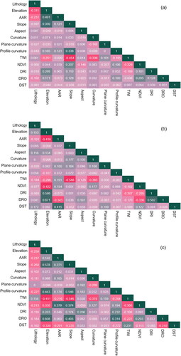
The training dataset was subjected to VIF and PCC tests as described above. As shown in Figure 5, the three railway lines present excellent multicollinearity detection results, with the maximum VIF value of 1.811 for elevation in XQ railway, 3.405 for elevation in southwest railway as well, and 2.456 for slope in GZ railway. Notably, all VIF values for each factor were below 5, indicating the suitability of all conditioning factors for landslide susceptibility modeling. Furthermore, the PCC value distribution exhibited distinct characteristics for the three railways, as presented in Figure 6. All PCC values remained below 0.7, confirming the absence of high correlation.

Figure 5. VIF testing results.

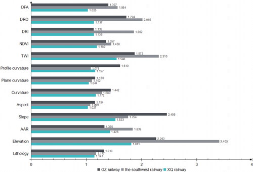
Figure 6. PCC testing: (a) XQ railway; (b) the southwest railway; (c) GZ railway.

4. Results

4.1. Models assessment and comparison

The application of side-sampling technique in analyzing the performance impact on models for XQ railway, the southwest railway, and GZ railway has significantly enhanced the models’ accuracy, precision, recall, F₁ score and ROC curve. For XQ railway, improvements were observed across all metrics, with accuracy, precision, recall, and F₁ Score increasing by 8.85%, 9.54%, 7.60%, and 8.57%, respectively. The southwest railway saw a notable rise in accuracy and F₁ Score by 12.11% and 24.89%, despite a slight drop in precision, yet recall surged from 0.529 to 0.882, a significant rise of 66.73%. GZ railway experienced increases in accuracy and F₁ Score by 15.61% and 10.87%, with precision improving by 20.92%, while recall remained stable at 0.864.

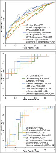
Moreover, the improvement in ROC curve values further substantiates the significant value of side-sampling technique. Specifically, the ROC curve value for the XQ railway increased from 0.707 to 0.760, marking a growth of 7.50%, while that for the southwest railway rose from 0.803 to 0.869, reflecting an increase of 8.22%. More notably, the ROC curve value for the GZ railway jumped from 0.678 to 0.842, achieving a surge of over 24%. This substantial enhancement demonstrates the potential of side-sampling method in marked boosting model performance. The analysis of these data not only highlights the pronounced effects of side-sampling method on improving the overall predictive capability of models but also emphasizes their widespread applicability and efficiency across various railway projects. For more detailed insights, refer to Table 2 and Figure 7.

Figure 7. ROC curves: (a) XQ railway; (b) the southwest railway; (c) GZ railway.

4.2. Models for landslide susceptibility mappings of three railways

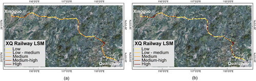
Using the four training models based on the side-sampling method, LSM were generated for the three railway lines. The choice of classification method often influences the spatial pattern distribution (Baeza et al. 2016). To facilitate a more intuitive analysis of the three railways, the equal interval method was employed to classify them into five categories: low, low-medium, medium, medium-high, and high susceptibility zones. The LSMs revealed a high degree of alignment between landslide locations and high or very high susceptibility zones. Three comparative figures (Figures 8–10) illustrate that the LSMs generated by two different sampling methods exhibit a high degree of similarity, indicating that datasets of landslides and non-landslides can effectively contribute to training. However, it is noteworthy that LSMs derived from side-sampling methods provide more definitive judgments on the potential hazards of railway lines, offering valuable insights for mitigating railway landslide hazards. For instance, in the case of the GZ railway, areas initially classified as medium risk or lower were reassessed as having higher danger levels after applying side-sampling methods; similarly, in the case of the southwest railway, particular attention was drawn to the routes in the eastern central region.

Figure 8. LSM of XQ railway: (a) original; (b) side-sampling.

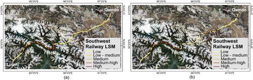
Figure 9. LSM of the southwest railway: (a) original; (b) side-sampling.

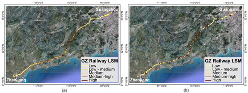
Figure 10. LSM of GZ railway: (a) original; (b) side-sampling.

5. Discussion

5.1. The universality of the side-sampling method

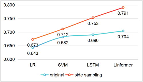
To accurately evaluate the performance enhancement potential of the side-sampling method, we employ four commonly used accuracy statistics based on the confusion matrix. The accuracy, a critical indicator for evaluating landslide susceptibility, directly reflects the model’s performance. As evident in Table 2, it is evident that the side-sampling method has a consistently positive impact on the accuracy of landslide susceptibility assessment across various typical models compared to the conventional approach, resulting in an impressive overall improvement of 7.68%. Specifically, the LR model applied to the XQ railway experiences the smallest uplift, at 1.60%, while the Linformer model applied to the GZ railway demonstrates the most substantial improvement, with a remarkable increase of 15.61%. Furthermore, precision consistently maintains a high level of consistency across the various evaluation metrics. Although a reduction in performance is observed for the Linformer model in the southwest railway, it is crucial to note that the average improvement for the remaining models stands at 7.19%, underscoring the effectiveness of the side-sampling method. Even in cases where the LSTM models for the XQ railway and GZ railway exhibit less favorable recall values, with a decline exceeding 3%, the average growth for the other models still achieves a noticeable increase of 13.48%. Notably, the side-sampling method significantly optimizes the accurate identification of landslides in the southwest railway. With the exception of the SVM model applied to the GZ railway, which experiences a performance decline of 2.91%, the average increase in the F₁ score for the remaining models reaches an impressive 9.92%.

Table 2. Data types and sources.

Data type	Data source	Data output type
Lithology	Geoscientific Data & Discovery Publishing System (http://dcc.cgs.gov.cn/)	Vector
Elevation	ASTER GDEM V3 (http://www.earthdata.nasa.gov)	Raster
AAR	National Center for Environmental Information (https://www.ncei.noaa.gov/)	Vector
Slope	DEM & ArcGIS10.5	Raster
Aspect	DEM & ArcGIS10.5	Raster
Curvature	DEM & ArcGIS10.5	Raster
Plane curvature	DEM & ArcGIS10.5	Raster
Profile curvature	DEM & ArcGIS10.5	Raster
TWI	DEM & ArcGIS10.5	Raster
NDVI	Geospatial data cloud & ArcGIS10.5	Raster
DRI	Geological and topographic maps	Vector
DRO	Geological and topographic maps	Vector
DST	Geological and topographic maps	Vector

In addition to the previous four indicators that can judge the model capability, the ROC curve was employed to further assess model performance. As can be seen from Figure 7, models based on the side-sampling method displayed a substantial overall improvement of approximately 6.22% relative to the original data, with the exception of a decrease observed in the LR model for the GZ railway.

Using four training models based on lateral sampling methods, LSMs for three railway lines were generated. As can be seen from the figures, the XQ railway exhibited intermittent regions of high landslide frequency in its northwest and south-central sections (Figure 11), while the central southwest area of the southwest railway (Figure 12) was identified as having a higher risk. The central portion of the GZ railway (Figure 13) exhibited greater instability compared to other regions. Despite minor variations in fine details due to differences in model accuracies, the LSMs effectively illustrated the distribution of potential landslides along the railway lines.

Figure 11. LSM of XQ railway: (a) LR; (b) SVM; (c) LSTM; (d) Linformer.

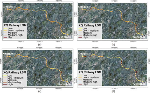
Figure 12. LSM of the southwest railway: (a) LR; (b) SVM; (c) LSTM; (d) Linformer.

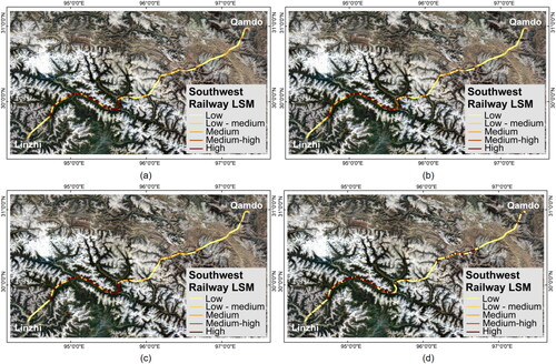
Figure 13. LSM of GZ railway: (a) LR; (b)SVM; (c) LSTM; (d) Linformer.

The three railways under study present unique situations, with the XQ railway having more landslide inventories than the GZ railway in the same source, the southwest railway having a similar number of landslides as the GZ railway but from a different source. Due to the larger dataset and more comprehensive model training, the overall average improvement in the XQ railway is slightly lower than that of the other two railways, while the data source of the southwest railway appears to better training effect of the side-sampling method. Therefore, it can be clearly seen that there are some deviations in the boosting of the side-sampling method for different data volumes, data sources and model types, but all of them have positive effects.

5.2. Performance improvement across different models

It is noteworthy that among the four models, the average accuracy of models trained using traditional data sampling methods ranks in descending order as Linformer, LSTM, SVM, and LR, which is consistent with the conclusion that deep learning models perform better than other models in previous articles exploring Linformer models (Jiang et al. 2023). Interestingly, deep learning models employing the side-sampling approach also exhibit significantly greater improvements compared to statistical and machine learning models, with the novel Linformer model outperforming the widely used LSTM model (Figure 14). Clearly, deep learning proves more suitable for training models in landslide susceptibility analysis, with the Linformer model demonstrating superior initial and enhanced learning capabilities. The Linformer model’s self-attention mechanism effectively captures dependencies, calculates the similarity between query and key, and optimizes weight distributions, showing enhanced capabilities.

Figure 14. Modelling capabilities of different sampling methods.

5.3. Sensitivity analysis of the optimal fixed area in the side-sampling method

In the above study, the side-sampling method with M = 3 was chosen to successfully improve the model’s landslide susceptibility assessment. Consequently, it is worthwhile to investigate whether capturing additional neighborhood unit features can further improve model performance. Given that the landslide inventories of the XQ railway significantly exceed those of the other two railways, resulting in less fluctuation in the training results of the original and side-sampled inventories, the XQ railway is chosen to assess the side-sampling method’s performance when M = 5.

Table 3 reveals that both M = 3 and M = 5 of the side-sampling method have their respective advantages and disadvantages across the five evaluation metrics mentioned above, with a slightly superior overall performance observed at M = 3. By comparing the original sampling method in Table 2 (i.e. the case of M = 1), it is evident that the side-sampling methods with M = 3 and M = 5 significantly outperform the original sampling. This result further demonstrates the effectiveness of side-sampling methods. It can be seen that when M = 5, each model tends to suffer from overfitting phenomenon, requiring more powerful arithmetic and consumes more time. Therefore, considering a comprehensive perspective, the side-sampling method with M = 3 is deemed suitable for model training to meet the training requirements.

Table 3. Comparison of M = 3 and M = 5 performance.

Indicators	LR (M = 3)	LR (M = 5)	SVM (M = 3)	SVM (M = 5)	LSTM (M = 3)	LSTM (M = 5)	Linformer (M = 3)	Linformer (M = 5)
ROC curve	0.617	0.615	0.748	0.752	0.737	0.719	0.760	0.753
Accuracy	0.573	0.573	0.667	0.667	0.688	0.673	0.726	0.707
Precision	0.571	0.571	0.663	0.667	0.699	0.679	0.735	0.691
Recall	0.602	0.596	0.683	0.671	0.665	0.658	0.708	0.752
F1 Score	0.586	0.584	0.673	0.669	0.682	0.669	0.722	0.720

6. Conclusion

In the assessment of landslide susceptibility, research on dataset often tends to be overlooked in comparison to studies on models algorithms, the balance of positive and negative samples, and the selection of non-landslide samples. This study introduces the side-sampling method into landslide susceptibility assessment based on the features of data augmentation and geographic clustering. The principles of the side-sampling method are elaborated in detail, and a systematic comparative analysis is conducted between the side-sampling method and the conventional sampling method through case studies involving three railways situated in diverse regions of China. Concurrently, landslide susceptibility is predicted for these three railways using the equal interval method. The research findings demonstrate the positive impact of the dataset on landslide susceptibility issues, offering a novel conceptual framework for obtaining reasonable and effective evaluation outcomes.

The proposed side-sampling method substantially enhances model evaluation effectiveness. In comparison to the original dataset, there is an impressive overall improvement in accuracy of 7.68%. Additionally, with few exceptions, precision, recall, and F₁ scores experience average increases of 7.19%, 13.48%, and 9.92%, respectively. Moreover, the ROC curve also records an overall enhancement of 6.22%. The initial application of the side-sampling method in landslide susceptibility analysis has shown exceptional capture capabilities and significant advantages, proving its universality across different models, data volumes, and data sources. Owing to the self-attention mechanism, the Linformer model exhibits outstanding performance relative to other models, with the incorporation of the side-sampling method extending its previous advantages. Furthermore, in the case study of the XQ railway, the ability of the side-sampling method to collect information from neighborhood units was tested with M = 5. The results indicate that M = 3 meets the requirements for model training.

Despite this study’s enhancement of the results of model performance evaluation through the lateral sampling method.

Although this study’s enhancement of the results of model performance evaluation through the side-sampling method, the impact of the improved method on the conditioning factors has not been comprehensively explored. Based on this, the further study will track the weighting ratio of the model, aiming to further reveal the reasons behind the superior accuracy achieved by the side-sampling method and explain how the Linformer model release its exceptional performance for weighted summation evaluation. Moreover, adjusting the value of M based on the scale of the landslide presents a worthy direction for exploration. By analyzing the variation of the M value across landslides of different scales within the study area, it is possible to more effectively demonstrate the model’s performance, thereby yielding more precise landslide prediction outcomes.

Data availability statement

All the data, models or code generated or used in the present study are available from the corresponding author by request.

Disclosure statement

No potential conflict of interest was reported by the authors.

Additional information

Funding

This study was financially supported by the National Natural Science Foundation of China (Grant No. 52078493); the Natural Science Foundation of Hunan Province (Grant No. 2022JJ30700); the Natural Science Foundation for Excellent Young Scholars of Hunan (Grant No. 2021JJ20057); the Science and Technology Plan Project of Changsha (Grant No. kq2305006), and the Innovation Driven Program of Central South University (Grant No. 2023CXQD033). These financial supports are gratefully acknowledged.

Appendix 1.

XQ railway conditioning factors

Appendix 2.

The southwest railway conditioning factors

Appendix 3.

GZ railway conditioning factors

References

- Abedini M, Ghasemian B, Shirzadi A, Shahabi H, Chapi K, Pham BT, Bin Ahmad B, Tien Bui D. 2019. A novel hybrid approach of Bayesian logistic regression and its ensembles for landslide susceptibility assessment. Geocarto Int. 34(13):1427–1457. doi: 10.1080/10106049.2018.1499820.
- Ado M, Amitab K, Maji AK, Jasińska E, Gono R, Leonowicz Z, Jasiński M. 2022. Landslide susceptibility mapping using machine learning: a literature survey. Remote Sens (Basel). 14(13):3029. doi: 10.3390/rs14133029.
- Agrawal K, Baweja Y, Dwivedi D, Saha R, Prasad P, Agrawal S, Kapoor S, Chaturvedi P, Mali N, Kala VU, et al. 2017. A comparison of class imbalance techniques for real-world landslide predictions. In: Proceedings - 2017 International Conference on Machine Learning and Data Science, MLDS 2017. Vol. 2018-January. doi: 10.1109/MLDS.2017.21.
- Agrawal N, Dixit J. 2022. Assessment of landslide susceptibility for Meghalaya (India) using bivariate (frequency ratio and Shannon entropy) and multi-criteria decision analysis (AHP and fuzzy-AHP) models. All Earth. 34(1):179–201. doi: 10.1080/27669645.2022.2101256.
- Akgun A, Dag S, Bulut F. 2008. Landslide susceptibility mapping for a landslide-prone area (Findikli, NE of Turkey) by likelihood-frequency ratio and weighted linear combination models. Environ Geol. 54(6):1127–1143. doi: 10.1007/s00254-007-0882-8.
- Akinci H, Zeybek M. 2021. Comparing classical statistic and machine learning models in landslide susceptibility mapping in Ardanuc (Artvin), Turkey. Nat Hazards. 108(2):1515–1543. doi: 10.1007/s11069-021-04743-4.
- Al-Najjar HAH, Pradhan B, Sarkar R, Beydoun G, Alamri A. 2021. A new integrated approach for landslide data balancing and spatial prediction based on generative adversarial networks (GAN). Remote Sens (Basel). 13(19):4011. doi: 10.3390/rs13194011.
- Avand M, Janizadeh S, Tien Bui D, Pham VH, Ngo PTT, Nhu VH. 2020. A tree-based intelligence ensemble approach for spatial prediction of potential groundwater. Int J Digit Earth. 13(12):1408–1429. doi: 10.1080/17538947.2020.1718785.
- Ayalew L, Yamagishi H. 2005. The application of GIS-based logistic regression for landslide susceptibility mapping in the Kakuda-Yahiko Mountains, Central Japan. Geomorphology. 65(1-2):15–31. doi: 10.1016/j.geomorph.2004.06.010.
- Azarafza M, Azarafza M, Akgün H, Atkinson PM, Derakhshani R. 2021. Deep learning-based landslide susceptibility mapping. Sci Rep. 11(1). doi: 10.1038/s41598-021-03585-1.
- Baeza C, Lantada N, Amorim S. 2016. Statistical and spatial analysis of landslide susceptibility maps with different classification systems. Environ Earth Sci. 75(19) doi: 10.1007/s12665-016-6124-1.
- Bahrami Y, Hassani H, Maghsoudi A. 2021. Landslide susceptibility mapping using AHP and fuzzy methods in the Gilan province, Iran. GeoJournal. 86(4):1797–1816. doi: 10.1007/s10708-020-10162-y.
- Bao S, Liu J, Wang L, Zhao X. 2022. Application of transformer models to landslide susceptibility mapping. Sensors (Basel). 22(23):9104. doi: 10.3390/s22239104.
- Bhagya SB, Sumi AS, Balaji S, Danumah JH, Costache R, Rajaneesh A, Gokul A, Chandrasenan CP, Quevedo RP, Johny A, et al. 2023. Landslide susceptibility assessment of a part of the Western Ghats (India) employing the AHP and F-AHP models and comparison with existing susceptibility maps. Land (Basel). 12(2):468. doi: 10.3390/land12020468.
- Bourenane H, Bouhadad Y, Guettouche MS, Braham M. 2015. GIS-based landslide susceptibility zonation using bivariate statistical and expert approaches in the city of Constantine (Northeast Algeria). Bull Eng Geol Environ. 74(2):337–355. doi: 10.1007/s10064-014-0616-6.
- Brenning A. 2005. Spatial prediction models for landslide hazards: review, comparison and evaluation. Nat Hazards Earth Syst Sci. 5(6):853–862. doi: 10.5194/nhess-5-853-2005.
- Broeckx J, Vanmaercke M, Duchateau R, Poesen J. 2018. A data-based landslide susceptibility map of Africa. Earth Sci Rev. 185:102–121. doi: 10.1016/j.earscirev.2018.05.002.
- Cao Y, Jia H, Xiong J, Cheng W, Li K, Pang Q, Yong Z. 2020. Flash flood susceptibility assessment based on geodetector, certainty factor, and logistic regression analyses in Fujian province, China. IJGI. 9(12):748. doi: 10.3390/ijgi9120748.
- Chang Z, Huang F, Huang J, Jiang SH, Liu Y, Meena SR, Catani F. 2023. An updating of landslide susceptibility prediction from the perspective of space and time. Geosci Front. 14(5):101619. doi: 10.1016/j.gsf.2023.101619.
- Chen C, Fan L. 2023. Selection of contributing factors for predicting landslide susceptibility using machine learning and deep learning models. Stoch Environ Res Risk Assess. doi: 10.1007/s00477-023-02556-4.
- Chi F, Han H. 2023. The impact of high-speed rail on economic development: a county-level analysis. Land (Basel). 12(4):874. doi: 10.3390/land12040874.
- Dang VH, Hoang ND, Nguyen LMD, Bui DT, Samui P. 2020. A novel GIS-Based random forest machine algorithm for the spatial prediction of shallow landslide susceptibility. Forests. 11(1):118. doi: 10.3390/f11010118.
- Dou J, Yunus AP, Bui DT, Merghadi A, Sahana M, Zhu Z, Chen CW, Han Z, Pham BT. 2020. Improved landslide assessment using support vector machine with bagging, boosting, and stacking ensemble machine learning framework in a mountainous watershed, Japan. Landslides. 17(3):641–658. doi: 10.1007/s10346-019-01286-5.
- Erener A, Sivas AA, Selcuk-Kestel AS, Düzgün HS. 2017. Analysis of training sample selection strategies for regression-based quantitative landslide susceptibility mapping methods. Comput Geosci. 104:62–74. doi: 10.1016/j.cageo.2017.03.022.
- Feizizadeh B, Jankowski P, Blaschke T. 2014. A GIS based spatially-explicit sensitivity and uncertainty analysis approach for multi-criteria decision analysis. Comput Geosci. 64:81–95. doi: 10.1016/j.cageo.2013.11.009.
- Florinsky IV. 1998. Accuracy of local topographic variables derived from digital elevation models. Intern J Geograph Inform Sci. 12(1):47–62. doi: 10.1080/136588198242003.
- Fu B, Li Y, Han Z, Fang Z, Chen N, Hu G, Wang W. 2023. RIPF-Unet for regional landslides detection: a novel deep learning model boosted by reversed image pyramid features. Nat Hazards. 119(1):701–719. doi: 10.1007/s11069-023-06145-0.
- Gao H, Fam PS, Tay LT, Low HC. 2020. Three oversampling methods applied in a comparative landslide spatial research in Penang Island, Malaysia. SN Appl Sci. 2(9) doi: 10.1007/s42452-020-03307-8.
- Ghorbanzadeh O, Blaschke T. 2019. Optimizing sample patches selection of CNN to improve the MIOU on landslide detection. In: GISTAM 2019 - Proceedings of the 5th International Conference on Geographical Information Systems Theory, Applications and Management. doi: 10.5220/0007675300330040.
- Ghorbanzadeh O, Xu Y, Ghamisi P, Kopp M, Kreil D. 2022. Landslide4Sense: reference Benchmark Data and Deep Learning Models for Landslide Detection. IEEE Trans Geosci Remote Sensing. 60:1–17. doi: 10.1109/TGRS.2022.3215209.
- Ghorbanzadeh O, Xu Y, Zhao H, Wang J, Zhong Y, Zhao D, Zang Q, Wang S, Zhang F, Shi Y, et al. 2022. The outcome of the 2022 Landslide4Sense competition: advanced landslide detection from multisource satellite imagery. IEEE J Sel Top Appl Earth Observations Remote Sensing. 15:9927–9942. doi: 10.1109/JSTARS.2022.3220845.
- Guzzetti F, Reichenbach P, Ardizzone F, Cardinali M, Galli M. 2006. Estimating the quality of landslide susceptibility models. Geomorphology. 81(1-2):166–184. doi: 10.1016/j.geomorph.2006.04.007.
- Habumugisha JM, Chen N, Rahman M, Islam MM, Ahmad H, Elbeltagi A, Sharma G, Liza SN, Dewan A. 2022. Landslide susceptibility mapping with deep learning algorithms. Sustainability (Switzerland.). 14(3):1734. doi: 10.3390/su14031734.
- Hamedi H, Alesheikh AA, Panahi M, Lee S. 2022. Landslide susceptibility mapping using deep learning models in Ardabil province, Iran. Stoch Environ Res Risk Assess. 36(12):4287–4310. doi: 10.1007/s00477-022-02263-6.
- He K, Gan C, Li Z, Rekik I, Yin Z, Ji W, Gao Y, Wang Q, Zhang J, Shen D. 2023. Transformers in medical image analysis. Intel Med. 3(1):59–78. doi: 10.1016/j.imed.2022.07.002.
- Huang F, Chen J, Liu W, Huang J, Hong H, Chen W. 2022. Regional rainfall-induced landslide hazard warning based on landslide susceptibility mapping and a critical rainfall threshold. Geomorphology. 408:108236. doi: 10.1016/j.geomorph.2022.108236.
- Huang W, Ding M, Li Z, Yu J, Ge D, Liu Q, Yang J. 2023. Landslide susceptibility mapping and dynamic response along the Sichuan-Tibet transportation corridor using deep learning algorithms. Catena (Amst). 222:106866. doi: 10.1016/j.catena.2022.106866.
- Huang Y, Zhao L. 2018. Review on landslide susceptibility mapping using support vector machines. Catena (Amst). 165:520–529. doi: 10.1016/j.catena.2018.03.003.
- Jiang N, Li Y, Han Z, Li J, Fu B, Yang J. 2023. A dataset-enhanced Linformer model for geo-hazards susceptibility assessment: a case study of the railway in Southwest China. Environ Earth Sci. 82(17) doi: 10.1007/s12665-023-11080-1.
- Kalantar B, Pradhan B, Amir Naghibi S, Motevalli A, Mansor S. 2018. Assessment of the effects of training data selection on the landslide susceptibility mapping: a comparison between support vector machine (SVM), logistic regression (LR) and artificial neural networks (ANN). Geomatics Nat Hazards Risk. 9(1):49–69. doi: 10.1080/19475705.2017.1407368.
- Kalyan KS, Rajasekharan A, Sangeetha S. 2022. AMMU: a survey of transformer-based biomedical pretrained language models. J Biomed Inform. 126:103982. doi: 10.1016/j.jbi.2021.103982.
- Kavzoglu T, Sahin EK, Colkesen I. 2014. Landslide susceptibility mapping using GIS-based multi-criteria decision analysis, support vector machines, and logistic regression. Landslides. 11(3):425–439. doi: 10.1007/s10346-013-0391-7.
- Kavzoglu T, Teke A. 2022. Predictive performances of ensemble machine learning algorithms in landslide susceptibility mapping using random forest, extreme gradient boosting (XGBoost) and Natural Gradient Boosting (NGBoost). Arab J Sci Eng. 47(6):7367–7385. doi: 10.1007/s13369-022-06560-8.
- Kim HI, Kim BH. 2020. Flood hazard rating prediction for urban areas using random forest and LSTM. KSCE J Civ Eng. 24(12):3884–3896. doi: 10.1007/s12205-020-0951-z.
- King G, Zeng L. 2003. Logistic regression in rare events data. J Stat Soft. 8(2) doi: 10.18637/jss.v008.i02.
- LeCun Y, Bengio Y, Hinton G. 2015. Deep learning. Nature. 521(7553):436–444. doi: 10.1038/nature14539.
- Li Y, Yang J, Han Z, Li J, Wang W, Chen N, Hu G, Huang J. 2023. An ensemble deep-learning framework for landslide susceptibility assessment using multiple blocks: a case study of Wenchuan area, China. Geomatics Nat Hazards Risk. 14(1) doi: 10.1080/19475705.2023.2221771.
- Li Z, Shi A, Li X, Dou J, Li S, Chen T, Chen T. 2024. Deep learning-based landslide recognition incorporating deformation characteristics. Remote Sens (Basel). 16(6):992. doi: 10.3390/rs16060992.
- Lin Q, Lima P, Steger S, Glade T, Jiang T, Zhang J, Liu T, Wang Y. 2021. National-scale data-driven rainfall induced landslide susceptibility mapping for China by accounting for incomplete landslide data. Geosci Front. 12(6):101248. doi: 10.1016/j.gsf.2021.101248.
- Liu M, Liu J, Xu S, Zhou T, Ma Y, Zhang F, Konečný M. 2021. Landslide susceptibility mapping with the fusion of multi-feature SVM model based FCM sampling strategy: a case study from Shaanxi Province. Int J Image Data Fusion. 12(4):349–366. doi: 10.1080/19479832.2021.1961316.
- Liu R, Li L, Pirasteh S, Lai Z, Yang X, Shahabi H. 2021. The performance quality of LR, SVM, and RF for earthquake-induced landslides susceptibility mapping incorporating remote sensing imagery. Arab J Geosci. 14(4) doi: 10.1007/s12517-021-06573-x.
- Liu S, Wang L, Zhang W, He Y, Pijush S. 2023. A comprehensive review of machine learning-based methods in landslide susceptibility mapping. Geol J. 58(6):2283–2301. doi: 10.1002/gj.4666.
- Lu W, Hu Y, Shao W, Wang H, Zhang Z, Wang M. 2024. A multiscale feature fusion enhanced CNN with the multiscale channel attention mechanism for efficient landslide detection (MS2LandsNet) using medium-resolution remote sensing data. Int J Digit Earth. 17(1) doi: 10.1080/17538947.2023.2300731.
- Lv Z, Zhang P, Benediktsson JA. 2017. Automatic object-oriented, spectral-spatial feature extraction driven by Tobler’s first law of geography for very high resolution aerial imagery classification. Remote Sens (Basel). 9(3):285. doi: 10.3390/rs9030285.
- Markham K, Frazier AE, Singh KK, Madden M. 2023. A review of methods for scaling remotely sensed data for spatial pattern analysis. Landsc Ecol. 38(3):619–635. doi: 10.1007/s10980-022-01449-1.
- Merghadi A, Abderrahmane B, Tien Bui D. 2018. Landslide susceptibility assessment at Mila basin (Algeria): a comparative assessment of prediction capability of advanced machine learning methods. IJGI. 7(7):268. doi: 10.3390/ijgi7070268.
- Merghadi A, Yunus AP, Dou J, Whiteley J, ThaiPham B, Bui DT, Avtar R, Abderrahmane B. 2020. Machine learning methods for landslide susceptibility studies: a comparative overview of algorithm performance. Earth Sci Rev. 207:103225. doi: 10.1016/j.earscirev.2020.103225.
- Moore ID, Grayson RB, Ladson AR. 1991. Digital terrain modelling: a review of hydrological, geomorphological, and biological applications. Hydrol Process. 5(1). doi: 10.1002/hyp.3360050103.
- Nam K, Wang F. 2019. The performance of using an autoencoder for prediction and susceptibility assessment of landslides: a case study on landslides triggered by the 2018 Hokkaido Eastern Iburi earthquake in Japan. Geoenviron Disasters. 6(1). doi: 10.1186/s40677-019-0137-5.
- Nami MH, Jaafari A, Fallah M, Nabiuni S. 2018. Spatial prediction of wildfire probability in the Hyrcanian ecoregion using evidential belief function model and GIS. Int J Environ Sci Technol. 15(2):373–384. doi: 10.1007/s13762-017-1371-6.
- Nefeslioglu HA, Gokceoglu C, Sonmez H. 2008. An assessment on the use of logistic regression and artificial neural networks with different sampling strategies for the preparation of landslide susceptibility maps. Eng Geol. 97(3-4):171–191. doi: 10.1016/j.enggeo.2008.01.004.
- Nikoobakht S, Azarafza M, Akgün H, Derakhshani R. 2022. Landslide susceptibility assessment by using convolutional neural network. Applied Sciences (Switzerland). 12(12):5992. doi: 10.3390/app12125992.
- Peng J, Cui P, Zhuang J. 2020. Challenges to engineering geology of Sichuan-Tibet railway. Yanshilixue Yu Gongcheng Xuebao/Chinese J Rock Mech Engng. 39(12). doi: 10.13722/j.cnki.jrme.2020.0446.
- Pham BT, Bui DT, Indra P, Dholakia MB. 2015. Landslide susceptibility assessment at a part of Uttarakhand Himalaya, India using GIS–based statistical approach of frequency ratio method. Int J Eng Res Technol. 4(11):338–344.
- Pham BT, Prakash I, Chen W, Ly HB, Ho LS, Omidvar E, Tran VP, Bui DT. 2019. A novel intelligence approach of a sequential minimal optimization-based support vector machine for landslide susceptibility mapping. Sustainability (Switzerland). 11(22, 6323). doi: 10.3390/su11226323.
- Pourghasemi HR, Kornejady A, Kerle N, Shabani F. 2020. Investigating the effects of different landslide positioning techniques, landslide partitioning approaches, and presence-absence balances on landslide susceptibility mapping. Catena (Amst). 187:104364. doi: 10.1016/j.catena.2019.104364.
- Qiao B, Zhu L, Yang R. 2019. Temporal-spatial differences in lake water storage changes and their links to climate change throughout the Tibetan Plateau. Remote Sens Environ. 222:232–243. doi: 10.1016/j.rse.2018.12.037.
- Reichenbach P, Rossi M, Malamud BD, Mihir M, Guzzetti F. 2018. A review of statistically-based landslide susceptibility models. Earth Sci Rev. 180:60–91. doi: 10.1016/j.earscirev.2018.03.001.
- Riitters K. 2019. Pattern metrics for a transdisciplinary landscape ecology. Landscape Ecol. 34(9):2057–2063. doi: 10.1007/s10980-018-0755-4.
- Rong G, Li K, Han L, Alu S, Zhang J, Zhang Y. 2020. Hazard mapping of the rainfall-landslides disaster chain based on geodetector and Bayesian network models in Shuicheng County, China. Water (Switzerland). 12(9):2572. doi: 10.3390/w12092572.
- Saha S, Saha A, Hembram TK, Kundu B, Sarkar R. 2022. Novel ensemble of deep learning neural network and support vector machine for landslide susceptibility mapping in Tehri region, Garhwal Himalaya. Geocarto Int. 37(27):17018–17043. doi: 10.1080/10106049.2022.2120638.
- Sahin EK, Colkesen I, Acmali SS, Akgun A, Aydinoglu AC. 2020. Developing comprehensive geocomputation tools for landslide susceptibility mapping: LSM tool pack. Comput Geosci. 144:104592. doi: 10.1016/j.cageo.2020.104592.
- Sameen MI, Pradhan B, Lee S. 2020. Application of convolutional neural networks featuring Bayesian optimization for landslide susceptibility assessment. Catena (Amst). 186:104249. doi: 10.1016/j.catena.2019.104249.
- Satarzadeh E,Sarraf A,Hajikandi H,Sadeghian MS. 2022. Flood hazard mapping in western Iran: assessment of deep learning vis-à-vis machine learning models. Nat Hazards. 111:1355–1373.
- Shao X, Ma S, Xu C, Zhou Q. 2020. Effects of sampling intensity and non-slide/slide sample ratio on the occurrence probability of coseismic landslides. Geomorphology. 363:107222. doi: 10.1016/j.geomorph.2020.107222.
- Shao X, Xu C. 2022. Earthquake-induced landslides susceptibility assessment: A review of the state-of-the-art. Nat Hazards Res. 2(3):172–182. doi: 10.1016/j.nhres.2022.03.002.
- Shijin W, Yanqiang WEI, Chunhua NIU, Zahng Y. 2021. Integrated risk management of multi-hazard natural disasters on the Tibetan Plateau. Glacial Permafrost. 43(06):1848–1860.
- Sonker, Irjesh, Tripathi, Jayant Nath, Swarnim, Swarnim. 2022. Remote sensing and GIS-based landslide susceptibility mapping using frequency ratio method in Sikkim Himalaya. Quaternary Sci Adv., 100067. 8. doi: 10.1016/j.qsa.2022.100067.
- Tobler WR. 1970. A computer movie simulating urban growth in the Detroit region. Econ Geogr. 46:234. doi: 10.2307/143141.
- Tsangaratos P, Ilia I. 2016. Comparison of a logistic regression and Naïve Bayes classifier in landslide susceptibility assessments: the influence of models complexity and training dataset size. Catena (Amst). 145:164–179. doi: 10.1016/j.catena.2016.06.004.
- Vaswani A, Shazeer N, Parmar N, Uszkoreit J, Jones L, Gomez AN, Kaiser Ł, Polosukhin I. 2017. Attention is all you need. In: Adv Neural Inf Process Syst. 2017-December[place unknown].
- Wang S, Li BZ, Khabsa M, Fang H, Ma H. 2020. Linformer: self-attention with linear complexity. arXiv preprint arXiv:200604768.
- Wang S, Zhuang J, Mu J, Zheng J, Zhan J, Wang J, Fu Y. 2022. Evaluation of landslide susceptibility of the Ya’an–Linzhi section of the Sichuan–Tibet Railway based on deep learning. Environ Earth Sci. 81(9) doi: 10.1007/s12665-022-10375-z.
- Wang WD, Li J, Han Z. 2020. Comprehensive assessment of geological hazard safety along railway engineering using a novel method: a case study of the Sichuan-Tibet railway, China. Geomatics Nat Hazards Risk. 11(1):1–21. doi: 10.1080/19475705.2019.1699606.
- Wang Y, Wu X, Chen Z, Ren F, Feng L, Du Q. 2019. Optimizing the predictive ability of machine learning methods for landslide susceptibility mapping using smote for Lishui city in Zhejiang province, China. Int J Environ Res Public Health. 16(3) doi: 10.3390/ijerph16030368.
- Wang Z, Chen T, Zhu D, Jia K, Plaza A. 2023. RSEIFE: A new remote sensing ecological index for simulating the land surface eco-environment. J Environ Manage. 326(Pt A):116851. doi: 10.1016/j.jenvman.2022.116851.
- Weiss GM, Provost F. 2003. Learning when training data are costly: the effect of class distribution on tree induction. Jair. 19:315–354. doi: 10.1613/jair.1199.
- Wu J. 2004. Effects of changing scale on landscape pattern analysis: scaling relations. Landsc Ecol. 19(2):125–138. doi: 10.1023/B:LAND.0000021711.40074.ae.
- Xi C, Han M, Hu X, Liu B, He K, Luo G, Cao X. 2022. Effectiveness of Newmark-based sampling strategy for coseismic landslide susceptibility mapping using deep learning, support vector machine, and logistic regression. Bull Eng Geol Environ. 81(5). doi: 10.1007/s10064-022-02664-5.
- Xu S, Song Y, Hao X. 2022. A comparative study of shallow machine learning models and deep learning models for landslide susceptibility assessment based on imbalanced data. Forests. 13(11):1908. doi: 10.3390/f13111908.
- Yan C, Ren X, Cheng Y, Song B, Li Y, Tian W. 2020. Geomechanical issues in the exploitation of natural gas hydrate. Gondwana Res. 81:403–422. doi: 10.1016/j.gr.2019.11.014.
- Yang C, Liu LL, Huang F, Huang L, Wang XM. 2023. Machine learning-based landslide susceptibility assessment with optimized ratio of landslide to non-landslide samples. Gondwana Res. 123:198–216. doi: 10.1016/j.gr.2022.05.012.
- Yang Y, Yu W, Liu Z, Zhao L, Lu C, Wu M, Niu R. 2022. Optimization of the Landslide Susceptibility Model based on Deep Forest and Twice-Sample. In. Proceedings - 2022 Chinese Automation Congress, CAC 2022. Vol. 2022-January. [place unknown]. doi: 10.1109/CAC57257.2022.10055494.
- Yi Y, Zhang W, Xu X, Zhang Z, Wu X. 2022. Evaluation of neural network models for landslide susceptibility assessment. Int J Digit Earth. 15(1):934–953. doi: 10.1080/17538947.2022.2062467.
- Yong C, Peijun S. 2008. Natural disasters. Beijing: Beijing Normal University Press.
- Youssef AM, Pradhan B, Dikshit A, Al-Katheri MM, Matar SS, Mahdi AM. 2022. Landslide susceptibility mapping using CNN-1D and 2D deep learning algorithms: comparison of their performance at Asir Region, KSA. Bull Eng Geol Environ. 81(4). doi: 10.1007/s10064-022-02657-4.
- Yu X, Zhang K, Song Y, Jiang W, Zhou J. 2021. Study on landslide susceptibility mapping based on rock–soil characteristic factors. Sci Rep. 11(1). doi: 10.1038/s41598-021-94936-5.
- Zabihi M,Mirchooli F,Motevalli A,Khaledi Darvishan A,Pourghasemi HR,Zakeri MA,Sadighi F. 2018. Spatial modelling of gully erosion in Mazandaran Province, northern Iran. Catena. 161:1–13. 10.1016/j.catena.2017.10.010.
- Zeng Q, Yuan G, McSaveney M, Ma F, Wei R, Liao L, Du H. 2020. Timing and seismic origin of Nixu rock avalanche in southern Tibet and its implications on Nimu active fault. Eng Geol. 268:105522. doi: 10.1016/j.enggeo.2020.105522.
- Zhang W, Wu J, Zhan S, Pan B, Cai Y. 2021. Environmental geochemical characteristics and the provenance of sediments in the catchment of lower reach of Yarlung Tsangpo River, southeast Tibetan Plateau. Catena (Amst). 200:105150. doi: 10.1016/j.catena.2021.105150.
- Zhang Y, Yan Q. 2022. Landslide susceptibility prediction based on high-trust non-landslide point selection. IJGI. 11(7):398. doi: 10.3390/ijgi11070398.
- Zhao L, Wu X, Niu R, Wang Y, Zhang K. 2020. Using the rotation and random forest models of ensemble learning to predict landslide susceptibility. Geomatics Nat Hazards Risk. 11(1):1542–1564. doi: 10.1080/19475705.2020.1803421.
- Zhao P, Masoumi Z, Kalantari M, Aflaki M, Mansourian A. 2022. A GIS-based landslide susceptibility mapping and variable importance analysis using artificial intelligent training-based methods. Remote Sens (Basel). 14(1):211. doi: 10.3390/rs14010211.
- Zhou X, Wen H, Zhang Y, Xu J, Zhang W. 2021. Landslide susceptibility mapping using hybrid random forest with GeoDetector and RFE for factor optimization. Geosci Front. 12(5):101211. doi: 10.1016/j.gsf.2021.101211.
- Zhu D, Chen T, Wang Z, Niu R. 2021. Detecting ecological spatial-temporal changes by remote sensing ecological index with local adaptability. J Environ Manage. 299:113655. doi: 10.1016/j.jenvman.2021.113655.
- Zhu D, Chen T, Zhen N, Niu R. 2020. Monitoring the effects of open-pit mining on the eco-environment using a moving window-based remote sensing ecological index. Environ Sci Pollut Res. 27(13):15716–15728. doi: 10.1007/s11356-020-08054-2.
- Zhuo L, Huang Y, Zheng J, Cao J, Guo D. 2023. Landslide susceptibility mapping in Guangdong Province, China, using random forest model and considering sample type and balance. Sustainability (Switzerland). 15(11):9024. doi: 10.3390/su15119024.